The Decay $B\to K^{*}\gamma$ from QCD Sum Rules

Abstract

Using the QCD sum rules approach and the complete leading–logarithmic short–distance coefficients determining the penguin–amplitude, we obtain $B(B\to K^{*}\gamma)=(6.8\pm 2.4)\cdot 10^{-5}$ for top–quark masses in the range (150–200) GeV and $|V_{cb}|=0.035$ for $\tau_{B}=1.5\,\text{ps}$. The ratio to the inclusive rate is $B(B\to K^{*}\gamma)/B(B\to X_{s}\gamma)=(20\pm 6)\%$.

Since some time, the penguin–induced decay $b\to s\gamma$ has received continuous interest as a possible probe of new physics (cf. e.g. [1, 2, 3]). The interest quite naturally increased when experimental results on the exclusive radiative decay $B\to K^{*}\gamma$ became available [4]. The interpretation of these results, however, is not obvious, since existing calculations focused mainly on the inclusive decay $B\to X_{s}\gamma$ with inidentified strange hadrons $X_{s}$ in the final state. The rate of this decay can be obtained from the perturbatively calculable short–distance expansion of the effective Hamiltonian. The existing estimates of hadronic corrections rely mainly on quark model [5, 6, 7] as well as QCD sum rule calculations [8, 9], and yield rather different results. To be specific, theory is asked to provide one with the hadronic matrix element $\langle\,K^{*}(p_{K^{*}})\,|\,\bar{s}\sigma_{\mu\nu}q^{\mu}Rb\,|\,B(p_{B})\,\rangle$ at vanishing momentum transfer squared, $q^{2}=(p_{B}-p_{K^{*}})^{2}=0$, where $R=(1+\gamma_{5})/2$ is the usual projector on right–handed quarks, and $\sigma_{\mu\nu}=i/2\,[\gamma_{\mu},\gamma_{\nu}]_{-}$. In this letter, we aim at to give an updated analysis of the exclusive decay $B\to K^{*}\gamma$, using both short–distance coefficients in leading–order accuracy [10] and improved QCD sum rules. We will not explain the QCD sum rules approach in detail, but just mention that it has established itself as a reliable tool to infer the gross features of QCD induced non–perturbative dynamics of hadronic matrix elements. The method relies on the field–theoretical aspects and features of QCD and was designed to make maximum use of known manifestations of non–perturbative QCD. Originally invented for the calculation of vacuum–to–meson transition amplitudes [11], it soon found application to the calculation of the electromagnetic form factor of the pion [12] and other meson–to–meson transition amplitudes (cf. [13] for a review). Although QCD sum rules in general yield less detailed results than fine–tuned models, they have the advantage that only a small number of parameters is needed that have an evident physical meaning (e.g. quark masses) and/or characterize the non–perturbative regime of QCD (e.g. the so–called quark condensate, the order parameter of chiral symmetry breaking). Once these parameters are fixed from well known processes, they can be used to calculate for instance heavy meson decays.

The decay we are interested in is determined by the effective Hamiltonian

$$H_{\text{eff}}=\frac{4G_{F}}{\sqrt{2}}\,V_{cb}V_{cs}^{*}\sum\limits_{i=1}^{8}C_{i}(\mu){\cal O}_{i}(\mu),$$ (1)

describing an effective five–quark theory where the effects of the top–quark and the W–boson are integrated out. The operators ${\cal O}_{i}$ mix under renormalization, their anomalous dimensions are known completely to leading–order and partly to next–to–leading order accuracy [1, 10, 14]. Since a calculation of $O(\alpha_{s})$ corrections to our sum rules is beyond the scope of this letter, we for consistency only use the leading–order coefficients calculated in [10].

The only operator relevant for the decay $B\to K^{*}\gamma$ is

$${\cal O}_{7}=\frac{e}{16\pi^{2}}\,\bar{s}\sigma_{\mu\nu}(m_{b}R+m_{s}L)bF^{\mu\nu}.$$ (2)

Here $m_{b}$ and $m_{s}$ are the masses of the b- and s-quark field, respectively, $F_{\mu\nu}$ is the electromagnetic field strength tensor, $L=(1-\gamma_{5})/2$ the projector on left–handed quarks. In calculating the decay rate, we note that the structure $\sigma_{\mu\nu}\gamma_{5}$ is not independent of $\sigma_{\mu\nu}$, but can be expressed as $\sigma_{\mu\nu}\gamma_{5}=-i\epsilon_{\mu\nu\alpha\beta}\sigma^{\alpha\beta}/2$, and thus the form factor decomposition of $\langle\,K^{*},\lambda\,|\,\bar{s}\sigma_{\mu\nu}q^{\mu}b\,|\,B\,\rangle$ determines the decay rate completely. With

$$\langle\,K^{*},\lambda\,|\,\bar{s}\sigma_{\mu\nu}q^{\mu}b\,|\,B\,\rangle=-iF(q^{2},\mu)\,\epsilon_{\alpha\nu\gamma\delta}\epsilon_{K^{*}}^{(\lambda)*\alpha}p_{B}^{\gamma}p_{K^{*}}^{\delta},$$ (3)

where $q=p_{B}-p_{K*}$ is the photon momentum, $\lambda$ denotes the helicity state of the K^∗ and $\epsilon^{(\lambda)}_{\mu}$ is the corresponding polarization vector, we find

$$\Gamma(B\to K^{*}\gamma)=\frac{\alpha}{128\pi^{4}}\,G_{F}^{2}\,|V_{cs}^{*}V_{cb}|^{2}\,C_{7}^{2}(\mu)F^{2}(0,\mu)(m_{b}^{2}+m_{s}^{2})\,\frac{(m_{B}^{2}-m_{K^{*}})^{3}}{m_{B}^{3}}\,.$$ (4)

In (3) and (4), we have made explicit the scale–dependence of the matrix element by ascribing the form factor a dependence on the normalization scale $\mu$. The inclusive rate is given by

$$\Gamma(B\to X_{s}\gamma)=\frac{\alpha}{32\pi^{4}}\,G_{F}^{2}\,|V_{cs}^{*}V_{cb}|^{2}\,C_{7}^{2}(\mu)\,m_{b}^{2}\,m_{B}^{3},$$ (5)

neglecting the s–quark mass.

In the framework of QCD sum rules, the form factor $F(0,\mu)$ can be calculated as ground state contribution to the three–point correlation function

$$T_{\alpha\nu}(p_{B}^{2},p_{K^{*}}^{2},q^{2}=0)=$$ (6)

$$= \left.i^{2}\!\!\int\!\!d^{4}\!x\,d^{4}\!y\,e^{-ip_{B}x+ip_{K^{*}}y}\,\langle\,0\,|\,T\,\bar{q}(y)\gamma_{\alpha}s(y)\,\bar{s}(0)q^{\mu}\sigma_{\mu\nu}b(0)\,\bar{b}(x)i\gamma_{5}q(x)\,|\,0\,\rangle\right|_{q^{2}=0}$$ (7)

$$= iT(p_{B}^{2},p_{K^{*}}^{2})\epsilon_{\alpha\nu\beta\gamma}p_{B}^{\beta}p_{K^{*}}^{\gamma}.$$ (8)

$T$ can be expressed as (double) dispersion relation where the double spectral function is given by the contribution of intermediate on–shell particles coupling to the currents. In zero–width approximation we find

$$T_{\alpha\nu}=-i\,F(0,\mu)\,\sum\limits_{\lambda}\frac{\langle\,0\,|\,\bar{q}\gamma_{\alpha}s\,|\,K^{*},\lambda\,\rangle\,\epsilon_{\alpha\nu\gamma\delta}\epsilon_{K^{*}}^{(\lambda)*\alpha}p_{B}^{\gamma}p_{K^{*}}^{\delta}\langle\,B\,|\,\bar{b}i\gamma_{5}q\,|\,0\,\rangle}{(p_{B}^{2}-m_{B}^{2})(p_{K^{*}}^{2}-m_{K^{*}}^{2})}+\text{continuum},$$ (9)

where the first term on the right–hand side just contains the expression we are interested in, the second one stands for the contributions of higher resonances and many–particle states. Introducing the meson leptonic decay constants $f_{B}$ and $f_{K^{*}}$ for the B and the K^∗ meson, respectively, as

$$\langle\,0\,|\,\bar{q}i\gamma_{5}b\,|\,B\,\rangle=\frac{m_{B}^{2}f_{B}}{m_{b}},\qquad\langle\,0\,|\,\bar{q}\gamma_{\mu}s\,|\,K^{*},\lambda\,\rangle=m_{K^{*}}f_{K^{*}}\epsilon_{\mu}^{(\lambda)},$$ (10)

we find

$$T=F(0,\mu)\,\frac{m_{K^{*}}f_{K^{*}}m_{B}^{2}f_{B}}{m_{b}}\,\frac{1}{(p_{B}^{2}-m_{B}^{2})(p_{K^{*}}^{2}-m_{K^{*}}^{2})}+\text{continuum}.$$ (11)

Using quark–hadron duality, we model the continuum part by the purely perturbative double spectral function above certain thresholds in the dispersion variables, the so–called continuum thresholds, $s_{B}^{0}$ and $s_{K^{*}}^{0}$, respectively. In order to enhance the contribution of the ground state and to suppress the continuum contribution, we subject $T$ to a Borel transformation $\hat{B}$ (cf. [11]) yielding

$$\hat{B}\,\frac{1}{s-p^{2}}=\frac{1}{M^{2}}\,e^{-s/M^{2}}.$$ (12)

By means of this transformation, the variable $p^{2}$ gets effectively replaced by $M^{2}$, the Borel parameter. Evidently, large values of the dispersion variable $s$, i.e. the continuum contribution, get exponentially suppressed.

Whereas $T$ is calculable within pure perturbation theory for $p_{B}^{2},\,p_{K^{*}}^{2}\to-\infty$ only, the QCD sum rules approach allows one to get closer to the more interesting physical region $p_{B}^{2}-m_{b}^{2}\approx p_{K^{*}}^{2}-m_{s}^{2}\approx 0$. Performing an operator product expansion of (8), it proves feasible to parametrize the unknown long–distance behaviour by vacuum expectation values of certain gauge–invariant operators, the so–called condensates [11]. These matrix elements vanish, when taken over the perturbative vacuum, but acquire finite values over the physical vacuum. Thus $T$ can be expressed as

$$T(p_{B}^{2},p_{K^{*}}^{2})=\sum_{n}T^{(n)}(p_{B}^{2},p_{K^{*}}^{2})\langle\,{\cal O}_{n}\,\rangle.$$ (13)

The coefficient functions $T^{(n)}$ contain the short–distance behaviour of the correlation function and are calculable perturbatively. In this letter we take into account all operators up to dimension n=6, i.e. the quark, gluon, mixed, and four–quark condensates. The evaluation of these contributions proceeds along standard lines, for the coefficient of the gluon condensate we use the method proposed in [15]. All coefficients are calculated to $O(\alpha_{s}^{0})$ and including their full dependence on $m_{s}$. For lack of space, we do not give the formulæ in this letter.

Applying the Borel transformation in both the variables $p_{B}^{2}$ and $p_{K^{*}}^{2}$, (11) yields the final sum rule

$$F(0,\mu)=\frac{m_{b}}{m_{K^{*}}f_{K^{*}}m_{B}^{2}f_{B}}\,e^{m_{B}^{2}/M_{B}^{2}+m_{K^{*}}^{2}/M_{K^{*}}^{2}}\,M_{B}^{2}M_{K^{*}}^{2}\,\hat{T}(M_{B}^{2},M_{K^{*}}^{2}).$$ (14)

Here $\hat{T}$ is the correlation function with subtracted continuum contribution, $M_{B}^{2}$ and $M_{K^{*}}$ are the Borel parameters. At this point, a few remarks are in order. First, the quark mass $m_{b}$ appearing in Eq. (14) is the renormalization scheme and group invariant pole mass, related to the running mass in the $\overline{\text{MS}}$ scheme by

$$m_{\text{pol}}=m_{\overline{\text{MS}}}(\mu)\left(1+\frac{\alpha_{s}(\mu)}{\pi}\,\left\{\frac{4}{3}+\ln\frac{\mu^{2}}{m^{2}_{\overline{\text{MS}}}}\right\}\right).$$ (15)

In the numerical evaluation we use the value $m_{b}=4.8\,\text{GeV}$. For the mass of the s–quark, we use the running $\overline{\text{MS}}$ mass with $m_{s}(\mu=1\,\text{GeV})=(0.20\pm 0.05)\,\text{GeV}$. Actually, the sum rule proves not very sensitive to that value. For the condensates, we use the standard set of values (at the renormalization point $\mu=1\,\text{GeV}$):

$$\langle\,\bar{q}q\,\rangle=(-0.24\,\text{GeV})^{3}\,, \langle\,\bar{q}g\sigma_{\mu\nu}G^{\mu\nu}q\,\rangle=0.8\,\text{GeV}^{2}\,\langle\,\bar{q}q\,\rangle,$$ (16)

$$\langle\,\alpha_{s}/\pi^{2}\,G^{2}\,\rangle=0.012\,\text{GeV}^{4}\,, \pi\alpha_{s}\langle\bar{q}\gamma^{\tau}\lambda^{A}q\sum_{u,d,s}\bar{q}\gamma_{\tau}\lambda^{A}q\rangle\approx-\frac{16}{9}\,\pi\alpha_{s}\langle\bar{q}q\rangle^{2},$$ (17)

$$4\pi\alpha_{s}\langle\bar{d}\bar{u}ud\rangle\approx 4\pi\alpha_{s}\langle\bar{q}q\rangle^{2}.$$ (18)

For $f_{K^{*}}$, we use the experimental value extracted from $\tau^{-}\to K^{*-}\nu_{\tau}$, $f_{K^{*}}=0.21\,\text{GeV}$ [16]. For $f_{B}$, we use a two–point sum rule (see [17], e.g.) without radiative corrections. In the limit of infinitely heavy quarks, this procedure is required to obtain the right normalization of the form factor [18], and largely reduces the dependence of the sum rule on the Borel parameter and the influence of (in our case unknown) radiative corrections [19]. We take over the procedure to the present case whith one light quark, and use half the value of the Borel parameter $M_{B}^{2}$ in the sum rule for $f_{B}$ and equal continuum thresholds $s_{B}^{0}$ in both the two– and the three–point sum rule. In addition, we evaluate (14) at a fixed ratio $M_{B}^{2}/M_{K^{*}}^{2}=3$. The numerical values of the continuum thresholds are taken from the region of maximum stability in the two–point sum rules, where one finds $s_{K^{*}}^{0}=1.7\,\text{GeV}^{2}$ and $s_{B}^{0}=34\,\text{GeV}^{2}$, and a “sum rule window” $7\,\text{GeV}^{2}\lesssim M_{B}^{2}\lesssim 10\,\text{GeV}^{2}$ (cf. [20, 21]).

Next, we have to say some words about the residual scale–dependence of $F(0,\mu)$. In contrast to calculations at partonic level, the condensates induce a scale–dependence of the sum rule already at leading order in $\alpha_{s}$. Whereas previous sum rule calculations tacitly assumed $\mu=m_{b}$ [8, 9], we argue that the effective scale is much below that. This becomes plausible when one takes into account that the sum rule calculation is an intrinsic off–shell one where the correlation function is calculated in the not so deep Euclidean region of external momenta and then analytically continued to the physical region. Thus the characteristic scale is rather given by the virtualities of the particle currents than by a singularity of the correlation function at threshold. Our reasoning gets support from the analysis of the heavy quark limit where the use of a low normalization scale $M^{2}/(2m_{Q})\approx 1\,\text{GeV}$ in the radiative corrections to the sum rule for $f_{B}$ is absolutely stringent [21]. From all that we conclude that the proper normalization scale of the sum rule is coupled to the Borel parameters. In view of the successes of previous form factor determinations ([20], e.g.), we conform to the choice made there and use $\mu=(M_{B}^{2}M_{K^{*}}^{2})^{1/4}$ which typically is about $2\,\text{GeV}$. Note that a further discussion of that point would require the complete calculation of $O(\alpha_{s})$ corrections to the correlation function which is complicated by the effects of operator mixing.

The next step now is to disentangle the intrinsic $M^{2}$–dependence of the sum rule for the form factor reflecting the inherent uncertainty of the QCD sum rule method from the scale–dependence induced by renormalization group. This amounts to scaling up $F(0,\mu)$ from the lower scale $\mu$ to, say, $m_{b}$. In doing so, we note that the complete solution of the renormalization group equation for ${\cal O}_{7}$,

$${\cal O}_{7}(m_{b})={\cal O}_{7}(\mu)\left[\frac{\alpha_{s}(m_{b})}{\alpha_{s}(\mu)}\right]^{16/(3\beta_{0})}+\sum\limits_{i\neq 7}\epsilon_{i}(\mu){\cal O}_{i}(\mu)$$ (19)

with coefficients $\epsilon_{i}(\mu)$ that describe the admixture of the other operators at $O(\alpha_{s})$, simplifies drastically for the matrix elements, since

$$\langle\,K^{*}\gamma\,|\,{\cal O}_{i}\,|\,B\,\rangle=0\quad\text{for\,}i\neq 7$$ (20)

at the specific scale $\mu$ and at one–loop level. Thus we have

$$F(0,m_{b})=F(0,\mu)\left[\frac{\alpha_{s}(m_{b})}{\alpha_{s}(\mu)}\right]^{16/(3\beta_{0})}.$$ (21)

Note, however, that although the initial condition for the solution of the renormalization group equation contains seven zeros (the matrix elements in (20)), all these matrix elements acquire non–zero values in scaling up to $m_{b}$ and contribute to the rate. In Fig. 2 we show $F(0,m_{b})$, calculated according to Eq. (14) and Eq. (21) as function of the Borel parameter $M_{B}^{2}$. The shaded area shows the working region of the sum rule, $7\,\text{GeV}^{2}\leq M_{B}^{2}\leq 10\,\text{GeV}^{2}$. Unfortunately, the sum rule is rather unstable against variation of the Borel parameter which is due to a relative sign between the contributions of the quark and the mixed condensate. This causes these contributions to be the dominant ones, whereas the perturbative contribution is rather small ($\sim 20\%$), the contribution of the gluon condensate and the four quark condensates are negligible ($\sim 2\%$). From the figure, we get

$$F(0,m_{b})=0.75\pm 0.10.$$ (22)

This value is smaller than the one obtained in previous analyses within the QCD sum rules approach [8, 9], and larger than the value obtained in [5, 6].

As mentioned before, it would be inconsistent to use this value for the determination of the decay rate. The correct procedure is to insert $F(0,\mu)$ as obtained from (14) into Eq. (4), using the same scale in the coefficient $C_{7}(\mu)$. For the combination $|V_{cb}|^{2}\,\tau_{B}$ that enters the formula for the branching ratio, we use the value $1.81\cdot 10^{-15}s$ obtained in [22] which amounts to $|V_{cb}|=0.035$ for the most recent determination $\tau_{B}=1.5\,\text{ps}$ of the B meson lifetime [23]. For the mass of the t-quark that dominates the penguin–amplitude we use the range of values $(150-200)\,\text{GeV}$ which is consistent with a recent determination of a lower bound on $m_{\text{top}}$ from low–energy data [24]. Taking all together, Eq. (4) yields the branching ratio $B(B\to K^{*}\gamma)$ plotted in Fig. 2 as a function of the Borel parameter $M_{B}^{2}$. Again we observe a rather strong dependence on $M_{B}^{2}$ which exceeds all other uncertainties in the input parameters of the sum rule, i.e. the quark masses and the values of the quark and the mixed condensate. Thus we get a branching ratio with large errors:

$$B(B\to K^{*}\gamma)=(6.8\pm 2.4)\cdot 10^{-5}$$ (23)

which coincides within the errors with the experimental value $B(B\to K^{*}\gamma)=(4.5\pm 1.5\pm 0.9)$. Taking the ratio of the exclusive to the inclusive decay rate, we obtain from Eqs. (4) and (5):

$$\frac{B(B\to K^{*}\gamma)}{B(B\to X_{s}\gamma)}=(20\pm 6)\%.$$ (24)

This value again is lower than the QCD sum rule results [8, 9] where values between 28% and 39% are given, but it is much larger than old constituent quark model results (4.5% [5], 6% [6]). It agrees with a recent analysis in [25] where $(13\pm 3)\%$ is obtained.

Concluding, we remark that although our results are by far not accurate enough as to impose constraints on $m_{\text{top}}$ or possible new physics, we find satisfying agreement of the QCD sum rule calculation for $B\to K^{*}\gamma$ with experiment. The main uncertainty of the sum rule calculation is caused by different signs in two major contributions which spoils the stability of the sum rule in the Borel parameter. Although this uncertainty might be reduced by including radiative corrections, their calculation proves prohibitively complicated.

Acknowledgement: The author thanks M. Misiak for useful discussions about the short–distance expansion for $b\to s\gamma$.

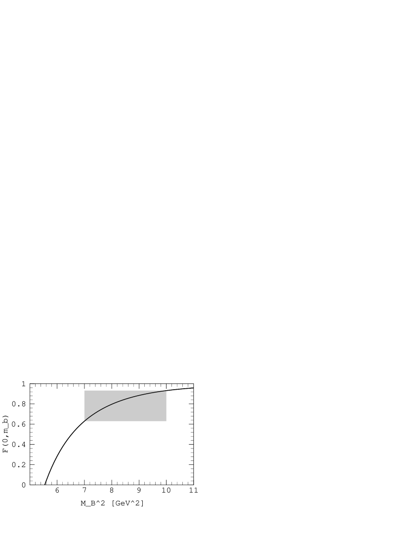
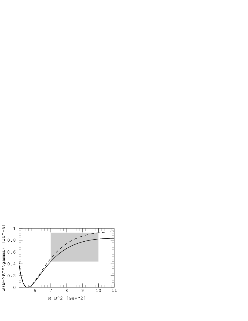
FIG. 1.: The form factor $F(0,m_{b})$ as function of the Borel parameter $M_{B}^{2}$ for $m_{b}=4.8\,\text{GeV}$, $m_{s}(1\,\text{GeV})=0.2\,\text{GeV}$ and continuum thresholds $s_{B}^{0}=34\,\text{GeV}^{2}$, $s_{K^{*}}^{0}=1.7\,\text{GeV}^{2}$, evaluated at a fixed ratio of the Borel parameters, $M_{B}^{2}/M_{K^{*}}^{2}=3$. The shaded area indicates the “sum rule window”.

FIG. 2.: The branching ratio $B(B\to K^{*}\gamma)$ as function of the Borel parameter $M_{B}^{2}$ with the same parameters as in Fig. 2. The shaded area again indicates the “sum rule window”. The solid line corresponds to $m_{\text{top}}=150\,\text{GeV}$, the dashed line to $m_{\text{top}}=200\,\text{GeV}$.

REFERENCES

- [1] B. Grinstein, R. Springer, M.B. Wise, Nucl. Phys. B 339, 269 (1990)
- [2] R. Barbieri, G.F. Giudice, Phys. Lett. B 309, 86 (1993)
- [3] L. Randall, R. Sundrum, Phys. Lett. B 312, 148 (1993)
- [4] R. Ammar et al. (CLEO–coll.), Phys. Rev. Lett. 71, 674 (1993)
- [5] T. Altomari, Phys. Rev. D 37, 677 (1988)
- [6] N.G. Deshpande, P. Lo, J. Trampetic, Z. Phys. C 40, 369 (1988)
- [7] A. Ali, C. Greub, Z. Phys. C 49, 431 (1991)
- [8] C.A. Dominguez, N. Paver, Riazuddin, Phys. Lett. B 214, 459 (1988)
- [9] T.M. Aliev, A.A. Ovchinnikov, V.A. Slobodenyuk, Phys. Lett. B 237, 569 (1990)
- [10] M. Misiak, Nucl. Phys. B 393, 23 (1993)
- [11] M.A. Shifman, A.I. Vainshtein, V.I. Zakharov, Nucl. Phys. B 147, 385, 448, 519 (1979)
- [12] B.L. Ioffe, A.V. Smilga, Nucl. Phys. B 216, 373 (1983)
- [13] Vacuum Structure and QCD Sum Rules, Current Physics Sources and Comments, Vol. 10, edited by M.A. Shifman (North–Holland, Amsterdam, 1992)
- [14] M. Misiak, Phys. Lett. B 269, 161 (1991)
- [15] P. Ball, TU München Preprint TUM–T31–39/93 (hep-ph/9305267), to appear in Phys. Rev. D
- [16] Particle Data Group, Phys. Rev. D 45 (1992)
- [17] T.M. Aliev, V.L. Eletskij, Sov. J. Nucl. Phys. 38, 936 (1983)
- [18] A.V. Radyushkin, Phys. Lett. B 271, 218 (1991)
- [19] E. Bagan, P. Ball, P. Gosdzinsky, Phys. Lett. B 301, 249 (1993)
- [20] P. Ball, V.M. Braun, H.G. Dosch, Phys. Rev. D 44, 3567 (1991)
- [21] E. Bagan et al., Phys. Lett. B 278, 457 (1992)
- [22] P. Ball, Phys. Lett. B 281, 133 (1992)
- [23] D. Buskulic et al. (ALEPH–coll.), Phys. Lett. B 307, 194 (1993); P.D. Acton et al. (OPAL–coll.), Phys. Lett. B 307, 247 (1993); P. Abreu et al. (DELPHI–coll.), Phys. Lett. B 312, 253 (1993)
- [24] A.J. Buras, TU München Preprint TUM–T31–45/93
- [25] A. Ali, C. Greub, DESY Preprint DESY 93–065 (1993)
- [26] M. Ciuchini et al., Preprint hep–ph/9307364