Constraints on SUSY Masses in Supersymmetric Grand Unified Theories
W. de Boer and R. Ehret
Inst. für Experimentelle Kernphysik, Univ. of Karlsruhe
Postfach 6980, D-76128 Karlsruhe 1, FRG
D.I. Kazakov
Joint Institute for Nuclear Research, Dubna
ABSTRACT

.

1. Introduction

Grand Unified Theories (GUT) hold the promise of ”explaining” the difference between the electromagnetic, weak and strong nuclear forces: their different strenghts are simply due to radiative corrections. Furthermore, they are candidates to explain several unrelated observations about our universe, e.g. they almost automatically lead to baryon number violation, thus providing a possible explanation for the matter-antimatter asymmetry in our universe[1] and the spontaneous symmetry breaking of the unified force into the known forces at a sufficient high energy can cause the inflationary scenario of the universe, thus providing an explanation for the origin of matter and the homogeneity of the universe on a large scale. The interested reader is refered to recent text books on this exciting subject [2] for more details and original references.

The $SU(5)$ group, which is the smallest group encompassing the $SU(3)$ and $SU(2)\bigotimes U(1)$ groups of the strong- and electroweak interactions, can be ruled out as a viable GUT, since it predicts too rapid proton decay. An upper limit on the proton lifetime can be estimated from the unification scale and any GUT is required to have the unification scale above $10^{15}$ GeV in order to be compatible with the proton life time limits. This is not the case in the SU(5) model and these limits severely constrain other GUT models.

Indeed, the coupling constants, as measured precisely at LEP, do not unify either within the $SU(5)$ model, i.e. they do not become equal at a single energy if extrapolated to high energies, but within the supersymmetric extension of the $SU(5)$ model (MSSM)[3], unification is obtained[4][5][6][7][8]. Supersymmetry[9] presupposes a symmetry between fermions and bosons, thus introducing spin 0 partners of the quarks and leptons – called squarks and sleptons – and spin 1/2 partners of the gauge bosons and Higgs particles – called gauginos and Higgsinos. Since these predicted particles have not been observed sofar, these supersymmetric (SUSY) particles must be heavier than the known particles, implying that supersymmetry must be broken. However, from the unification condition a first estimate of the SUSY breaking scale could be made: it was found to be of the order of 1000 GeV, or more precisely $10^{3\pm 1}$ GeV[5]. The uncertainty in this scale is mainly caused by the uncertainty in the strong coupling constant.

Clearly, the whole SUSY mass spectrum cannot be described by a single parameter. In the MSSM one needs at least 5 parameters. So many parameters cannot be derived from the unification condition alone. However, further constraints can be considered:

• $M_{Z}$ predicted from electroweak symmetry breaking[10][11].

• b-quark mass predicted from the unification of Yukawa couplings[12][11][13].

• Constraints from the lower limit on the proton lifetime[14][15][16].

• Constraints from the lower limit on the lifetime of the universe[17].

• The maximum value of the top mass is restricted by the couplings[11].

• Experimental lower limits on SUSY masses[18].

All these constraints have been considered separately or partly[4][5][6][7][8][15][19][20]. However, considering only one constraint at a time allows one to obtain only one relation between parameters. Trying to find complete solutions requires additional assumptions, like naturalness, no-scale models, fixed ratios for gaugino- and scalar masses or a fixed ratio for the Higgs mixing parameter and the scalar mass, assumptions from supergravity, or combinations of these assumptions.

The different assumptions lead sometimes to apparently conflicting results. For example, the dark matter constraint requires the mass of the scalar particles at $M_{GUT}$ to be below 500 GeV[17], while the analysis of the proton life time constraint requires this mass to be above 600 GeV[14].

It is the purpose of this paper to study all constraints simultaneously without any of the assumptions mentioned above in order to see if a solution within the minimal supersymmetric model (MSSM) exists at all, which is non-trivial as should be clear from the contradictions mentioned before.

It turns out that a solution exists indeed and the corresponding constraints on the SUSY mass spectrum, the strong coupling constant and the top mass are given, if all constraints from the experimental data mentioned above are imposed simultaneously (for the first time as fas as we know).

2. Experimental constraints

2.1. Unification of the couplings

In the unified $\rm SU(2)\bigotimes U(1)$ theory, the following well known tree-level relations hold between the couplings and the gauge boson masses

$$\matrix{e&=&\sqrt{4\pi\alpha}=g\sin\theta_{W}=g^{\prime}\cos\theta_{W}\cr M_{\rm W}&=&{1\over 2}vg\cr M_{\rm Z}&=&{1\over 2}v\sqrt{g^{\prime 2}+g^{2}}\cr}$$

from which it follows that

$$\sin^{2}\theta_{W}={e^{2}\over g^{2}}={g^{\prime 2}\over g^{\prime 2}+g^{2}}=1-{M_{\rm W}^{2}\over M_{\rm Z}^{2}}$$

Here $g$ and $g^{\prime}$ are the couplings of the groups SU(2) and U(1) respectively, $\alpha$ is the fine structure constant and $v$ is the vacuum expectation value of the Higgs field. If the model contains Higgs representations other than doublets, the theory has an additional degree of freedom, usually parametrized by the $\rho$ parameter.

In the SM based on the group $\rm SU(3)\times SU(2)\times U(1)$ we use the usual definitions of the couplings

$$\matrix{\alpha_{1}&=&(5/3)g^{\prime 2}/(4\pi)&=&5\alpha/(3\cos^{2}\theta_{W})\cr\alpha_{2}&=&\hfill g^{2}/(4\pi)&=&\alpha/\sin^{2}\theta_{W}\hfill\cr\alpha_{3}&=&\hfill g_{s}^{2}/(4\pi)\cr}$$

where $g_{s}$ is the SU(3) coupling. The factor of $5/3$ in the definition of $\alpha_{1}$ has been included for the proper normalization at the unification point[21]. The couplings, when defined as effective values including loop corrections in the gauge boson propagators, become energy dependent (“running”). A running coupling requires the specification of a renormalization prescription, for which one usually uses the modified minimal subtraction (${\overline{MS}}$) scheme[22].

In this scheme the world averaged values of the couplings at the Z⁰ energy are

$$\matrix{\alpha^{-1}(M_{\rm Z})&=&127.9\pm 0.2\cr\sin^{2}\theta_{\overline{MS}}&=&0.2326\pm 0.0006\cr\alpha_{3}&=&0.123\pm 0.008\cr}$$

The value of $\alpha^{-1}$ is given in Ref. [23] and the value of $\sin^{2}\theta_{\overline{MS}}$ has been presented at Marseille[24]. The $\alpha_{3}$ value corresponds to value measured at LEP form the ratio of the hadronic- and leptonic cross sections[25], which agrees well with the world average[26]. This value has the smallest theoretical uncertainty from the higher order corrections, we prefer to take this value alone.

For SUSY models, the dimensional reduction ${\overline{DR}}$ scheme is a more appropriate renormalization scheme[27]. This scheme also has the advantage that all thresholds can be treated by simple step approximations. Thus unification occurs in the ${\overline{DR}}$ scheme if all three $\alpha_{i}^{-1}(\mu)$ meet exactly at one point. This crossing point then gives the mass of the heavy gauge bosons. The ${\overline{MS}}$ and ${\overline{DR}}$ couplings differ by a small offset

$${1\over\alpha_{i}^{\overline{DR}}}={1\over\alpha_{i}^{\overline{MS}}}-{C_{i}\over 12\pi}$$

where the $C_{i}$ are the quadratic Casimir coefficients of the group ($C_{i}=N$ for SU($N$) and 0 for U(1) so $\alpha_{1}$ stays the same). Throughout the following, we use the ${\overline{DR}}$ scheme for the MSSM.

The energy dependence of the couplings is completely determined by the particle content and their couplings inside the loop diagrams of the gauge bosons as expressed by the renormalization group (RG) equations. The RG equations can be rewritten as

$${d\over d\ln\mu}\alpha_{i}^{-1}(\mu)={-1\over 2\pi}\left(b_{i}+\sum_{j=1}^{3}{b_{ij}\over 4\pi}\alpha_{j}(\mu)+O(\alpha_{j}^{2})\right).$$

In first order, i.e. all $b_{ij}=0$, the equations for the three $\alpha_{i}^{-1}$ are independent with a linear solution in the $\alpha_{i}^{-1}$—$\log\mu$ plane. When the second order contributions are taken into account, the equations become coupled and the running of each $\alpha_{i}^{-1}$ depends on the values of the other two couplings. However, the second order effects are small because of the additional factor $\alpha_{j}/(4\pi)\leq 0.01$. Higher orders are presumably even smaller by additional powers of $\alpha_{j}/(4\pi)$. We solve (2.6) by numerical integration.

2.2. $M_{Z}$  constraint from electroweak symmetry breaking

In the MSSM at least two Higgs doublets have to be introduced:

$$H_{1}(1,2,-\frac{1}{2})=\left(\begin{array}[]{c}H^{0}_{1}\\ H^{-}_{1}\end{array}\right),\ \ \ H_{2}(1,2,\frac{1}{2})=\left(\begin{array}[]{c}H^{+}_{2}\\ H^{0}_{2}\end{array}\right),$$

At the tree level the interactions of the Higgs fields can be parametrised by an effective potential of the form:

$$V(H_{1},H_{2})=m^{2}_{1}|H_{1}|^{2}+m^{2}_{2}|H_{2}|^{2}-m^{2}_{3}(H_{1}H_{2}+h.c.)+\frac{g^{2}+g^{{}^{\prime}2}}{8}(|H_{1}|^{2}-|H_{2}|^{2})^{2},$$

where $m_{1}$, $m_{2}$ and $m_{3}$ are mass parameters, for which we assume at the GUT scale the following boundary conditions: $m_{1}^{2}=m^{2}_{2}=\mu^{2}_{0}+m_{0}^{2},\ m^{2}_{3}=B\mu_{0}m_{0}$.

Radiative corrections from the heavy top and stop quarks can drive one of the Higgs masses negative, thus causing spontaneous symmetry breaking in the electroweak sector. In this case the Higgs potential does not have its minimum for all fields equal zero, but the the minimum is obtained for non-zero vacuum expectation values of the fields:

$$<H_{1}>\equiv v_{1}=\frac{v}{\sqrt{2}}\cos\beta,\ \ <H_{2}>\equiv v_{2}=\frac{v}{\sqrt{2}}\sin\beta,$$

$$v^{2}=\frac{v_{1}^{2}+v_{2}^{2}}{2},\ \ \tan\beta\equiv\frac{v_{1}}{v_{2}}$$

The scale, where symmetry breaking occurs depends on the starting values of the mass parameters at the GUT scale, the top mass and the evolution of the couplings and masses. This gives strong constraints between the known $Z^{0}$ mass and the SUSY mass parameters, as demonstrated e.g. in Ref.[10].

Minimization of the tree level potential yields:

$$v^{2}=\frac{\displaystyle 8(m^{2}_{1}-m^{2}_{2}\tan^{2}\beta)}{\displaystyle(g^{2}+g^{{}^{\prime}2})(\tan^{2}\beta-1)},\ \ \ \sin 2\beta=\frac{\displaystyle 2m^{2}_{3}}{\displaystyle m^{2}_{1}+m^{2}_{2}}$$

$$M^{2}_{W}=\frac{g^{2}}{4}v^{2},\ \ M^{2}_{Z}=\frac{g^{2}+g^{{}^{\prime}2}}{4}v^{2},$$

After including the one-loop corrections to the potential[28], the $Z^{0}$ mass becomes dependent on the top- and stop quark masses too. In this case we derived the following expression:

$$M^{2}_{Z} = 2\frac{\displaystyle m^{2}_{1}-m^{2}_{2}\tan^{2}\beta-\Delta^{2}_{Z}}{\tan^{2}\beta-1},$$

$$\Delta^{2}_{Z} = \frac{3g^{2}}{32\pi^{2}}\frac{m^{2}_{t}}{M^{2}_{W}}\left[f(\tilde{m}^{2}_{t1})+f(\tilde{m}^{2}_{t2})+2m^{2}_{t}+(A^{2}_{t}-\mu^{2}\cot^{2}\beta)\frac{f(\tilde{m}^{2}_{t1})-f(\tilde{m}^{2}_{t2})}{\tilde{m}^{2}_{t1}-\tilde{m}^{2}_{t2}}\right]$$

where

$$f(m^{2})=m^{2}(\ln\frac{m^{2}}{m^{2}_{t}}-1),\ \ h(m^{2})=\frac{m^{2}}{m^{2}-\tilde{m}^{2}_{q}}\ln\frac{m^{2}}{\tilde{m}^{2}_{q}}$$

$$d(m^{2}_{1},m^{2}_{2})=2-\frac{m^{2}_{1}+m^{2}_{2}}{m^{2}_{1}-m^{2}_{2}}\ln\frac{m^{2}_{1}}{m^{2}_{2}}$$

$\tilde{m}^{2}_{q}$ is the mass of a light squark and $\tilde{m}^{2}_{1,2}$ the stop quark masses. Note that the corrections $\Delta_{Z}$ are zero if the top- and stop quark masses are identical, i.e. if supersymmetry would be exact. They grow with the difference $\tilde{m}^{2}_{t}-{m_{t}}^{2}$, so these corrections become unnaturally large for large values of the stop masses, as will be discussed later.

The masses of the physical Higgs particles after spontaneous symmetry breaking become after inclusion of the one-loop corrections[28]:

$$m^{2}_{A} = \frac{\Delta^{2}_{A}}{\sin 2\beta},$$

$$\Delta^{2}_{A} = 2m^{2}_{3}-\frac{3g^{2}}{16\pi^{2}}\frac{m^{2}_{t}A_{t}\mu}{\sin^{2}\beta M^{2}_{W}}\frac{f(\tilde{m}^{2}_{t1})-f(\tilde{m}^{2}_{t2})}{\tilde{m}^{2}_{t1}-\tilde{m}^{2}_{t2}}$$

$$m^{2}_{H^{\pm}} = m^{2}_{A}+M^{2}_{W}+\Delta^{2}_{H},$$

$$\Delta^{2}_{H} = -\frac{3g^{2}}{32\pi^{2}}\frac{m^{2}_{t}\mu^{2}}{\sin^{4}\beta M^{2}_{W}}\frac{h(\tilde{m}^{2}_{t1})-h(\tilde{m}^{2}_{t2})}{\tilde{m}^{2}_{t1}-\tilde{m}^{2}_{t2}}$$

$$m^{2}_{h,H} = \frac{1}{2}\left[m^{2}_{A}+M^{2}_{Z}+\Delta_{11}+\Delta_{22}\right.$$

$$\left.\pm\sqrt{\begin{array}[]{ll}(m^{2}_{A}+M_{Z}^{2}+\Delta_{11}+\Delta_{22})^{2}&-4m^{2}_{A}M_{Z}^{2}\cos^{2}2\beta-4(\Delta_{11}\Delta_{22}-\Delta_{12}^{2})\\ -4(\cos^{2}\beta M^{2}_{Z}+\sin^{2}\beta M^{2}_{A})\Delta_{22}&-4(\sin^{2}\beta M^{2}_{Z}+\cos^{2}\beta M^{2}_{A})\Delta_{11}\\ -4\sin 2\beta(M^{2}_{Z}+M^{2}_{A})\Delta_{12}&\end{array}}\right]$$

$$\Delta_{11} = \frac{3g^{2}}{16\pi^{2}}\frac{m^{4}_{t}}{\sin^{2}\beta M^{2}_{W}}\left[\frac{\mu(A_{t}+\mu\cot\beta)}{\tilde{m}^{2}_{t1}-\tilde{m}^{2}_{t2}}\right]^{2}d(\tilde{m}^{2}_{t1},\tilde{m}^{2}_{t2}),$$

$$\Delta_{22} = \frac{3g^{2}}{16\pi^{2}}\frac{m^{4}_{t}}{\sin^{2}\beta M^{2}_{W}}\left[\ln(\frac{\tilde{m}^{2}_{t1}\tilde{m}^{2}_{t2}}{m^{4}_{t}})+\frac{2A_{t}(A_{t}+\mu\cot\beta)}{\tilde{m}^{2}_{t1}-\tilde{m}^{2}_{t2}}\ln(\frac{\tilde{m}^{2}_{t1}}{\tilde{m}^{2}_{t2}})\right.$$

$$\left.\left[+\frac{A_{t}(A_{t}+\mu\cot\beta)}{\tilde{m}^{2}_{t1}-\tilde{m}^{2}_{t2}}\right]^{2}d(\tilde{m}^{2}_{t1},\tilde{m}^{2}_{t2})\right],$$

$$\Delta_{12} = \frac{3g^{2}}{16\pi^{2}}\frac{m^{4}_{t}}{\sin^{2}\beta M^{2}_{W}}\frac{\mu(A_{t}+\mu\cot\beta)}{\tilde{m}^{2}_{t1}-\tilde{m}^{2}_{t2}}\left[\ln(\frac{\tilde{m}^{2}_{t1}}{\tilde{m}^{2}_{t2}})+\frac{A_{t}(A_{t}+\mu\cot\beta)}{\tilde{m}^{2}_{t1}-\tilde{m}^{2}_{t2}}d(\tilde{m}^{2}_{t1},\tilde{m}^{2}_{t2})\right],$$

$$A(t) = \frac{\displaystyle A_{0}}{\displaystyle 1+6Y_{0}F(t)}+\frac{m_{1/2}}{m_{0}}\left(H_{2}-\frac{\displaystyle 6Y_{0}H_{3}}{\displaystyle 1+6Y_{0}F(t)}\right)$$

Here $H_{2},H_{3},E$ and $F$ are functions of the couplings as defined in [11].

2.3. Evolution of the masses

In the soft breaking term of the Lagrangian $m_{0}$  and $m_{1/2}$  are the universal masses of the gauginos and scalar particles at the GUT scale, respectively and $\mu$ determines the masses of the particles in the Higgs sector. At lower energies the masses of the SUSY particles start to differ from these universal masses due to the radiative corrections. E.g. the coloured particles get contributions proportional to ${\alpha_{s}}^{2}$ from gluon loops, while the non-coloured ones get contributions depending on the electroweak coupling constants only. The evolution of the masses is given by the renormalisation group equations[11]. We have used analytical solutions[29] of these equations including the top Yukawa coupling, the Higgs mass parameters, mass mixing between the top quarks, mixing between neutralinos, mixing between the charginos and one loop radiative corrections to the Higgs potential.

2.4. b-quark mass constraint

Unification of the Yukawa couplings for a given generation at the GUT scale predicts relations for quark and lepton masses within a given family. This does not work for the light quarks, but the ratio of b-quark and $\tau$-lepton masses can be correctly predicted by the radiative corrections to the masses[11].

2.5. Proton lifetime constraints

GUT’s predict proton decay and the present lower limits on the proton lifetime yield quite strong constraints on the GUT scale and the SUSY parameters. As mentioned at the beginning, the direct decay $p\rightarrow e^{+}\pi^{0}$ via s-channel exchange requires the GUT scale to be above $10^{15}$ GeV. This is not fulfilled in the SM, but always fulfilled in the MSSM. Therefore we do not consider this constraint. However, the decay via box diagrams with winos and Higgsinos predict much shorter lifetimes, especially in the preferred mode $p\rightarrow\overline{\nu}K^{+}$. From the present experimental lower limit of $10^{32}$ yr for this decay mode Arnowitt and Nath[14]  deduce an upper limit on the parameter B:

$$B<293\pm 42(M_{H_{3}}/3{M_{GUT}})\ GeV^{-1}$$

Here $M_{H_{3}}$ is the Higgsino mass, which is expected to be of the order of ${M_{GUT}}$. To obtain a conservative upper limit on $B$, we allow $M_{H_{3}}$ to become an order of magnitude heavier than ${M_{GUT}}$, so we require

$$B<977\pm 140\ GeV^{-1}.$$

The uncertainties from the unknown heavy Higgs mass are large compared with the contributions from the first and third generation, which contribute through the mixing in the CKM matrix. Therefore we only consider the second order generation contribution, which can be written as[14] :

$$B=-2(\alpha_{2}/(\alpha_{3}\sin(2\beta))(m_{\tilde{g}}/m^{2}_{\tilde{q}})~{}10^{6}$$

One observes that the upper limit on $B$ favours small gluino masses $m_{\tilde{g}}$, large squark masses $m_{\tilde{q}}$, and small values of $\tan\beta$. To fulfill this constraint requires

$${\tan\beta}<5$$

for the whole parameter space. Arnowitt and Nath note that requiring the gluino mass to be below 500 GeV implies the mass of the scalar particles ($m_{0}$) at the GUT scale to be above 600 GeV. We will not impose this requirement on the gluino mass. Furthermore, they require $M_{H_{3}}<3~{}{M_{GUT}}$, so they obtained tighter limits on $\tan\beta$, since we allow $M_{H_{3}}<10~{}{M_{GUT}}$.

2.6. t-quark mass constraints

For large Yukawa couplings the masses become dependent only on the couplings (pole term in the RGE). This yields a maximum value of the top mass, which has to be higher than the experimental mass, thus constraining the SUSY parameters. More precisely, the top mass can be expressed as:

$${m_{t}}^{2}=(4\pi)^{2}\ Y_{t}(t)\ v^{2}\ \sin^{2}(\beta)$$

where the running of the Yukawa coupling as function of $t=log(\frac{M_{X}^{2}}{Q^{2}})$ is given by[11]:

$$Y_{t}(t)=\frac{\displaystyle Y_{0}E(t)}{\displaystyle 1+6Y_{0}F(t)}$$

One observes that for large Yukawa couplings $Y_{0}$ at the GUT scale, $Y_{t}$ becomes independent of $Y_{0}$ and the maximum value of ${m_{t}}$ becomes:

$${m_{t}}^{2}=\frac{(4\pi)^{2}\ E(t)}{6F(t)}\ v^{2}\ \sin^{2}(\beta),$$

where $E$ and $F$ are functions of the couplings only[11]. Clearly the experimental values of ${m_{t}}$ have to be below this upper bound, which is most easily fulfilled for larger values of ${\tan\beta}$. However, the proton life time limits require ${\tan\beta}<5$, as discussed before. In this case the upper limit on ${m_{t}}$ implies a constraint on the ratio of $E/F$, i.e. on the starting point at the GUT scale and the intermediate SUSY thresholds.

2.7. Constraints from the lifetime of the universe

The lightest supersymmetric particle (LSP) is supposedly stable and would be an ideal candidate for dark matter. So the MSSM predicts dark matter. However, from the long lifetime of the universe one knows that the density of the universe cannot be higher than the critical density, which implies most of the LSP’s have annihilated into photons. This can only happen fast enough if the squarks and sleptons are sufficiently light, thus posing a strong upper limit on some of the SUSY mass parameters. Requiring the density of the universe to be below the critical density translates into an upper bound of about 500 GeV on $m_{0}$  for a large range of $m_{1/2}$[17], i.e.

$${m_{0}}<500~{}GeV.$$

2.8. Experimetal lower limits on SUSY masses

SUSY particles have not been found sofar and from the searches at LEP one knows that the lower limit on the charged particles is about half the $Z^{0}$  mass (45 GeV) and the Higgs mass has to be above 60 GeV[18]. This requires also minimal values for the SUSY mass parameters.

3. Constrained Fits

3.1. Fit strategy

As mentioned before, given the 5 parameters in the MSSM and ${\alpha_{GUT}}$ and ${M_{GUT}}$, all other SUSY masses, the b-quark mass, $M_{Z}$, and the proton lifetime can be calculated. In addition, the complete evolution of the couplings including all thresholds can be performed. Furthermore, the dark matter constraint requires $m_{0}$ to be below 500 GeV.

Therefore we have adopted the following strategy: we varied $m_{0}$ between 0 and 500 GeV and fitted the remaining 5 parameters: ${\alpha_{GUT}},\ {M_{GUT}},\ {m_{1/2}},\ \mu,\$ and ${\tan\beta}$. The trilinear coupling $A_{0}$ in the Higgs potential at ${M_{GUT}}$ was kept mostly at 0, but the large radiative corrections to it were taken into account for the top quarks. Varying $A_{0}$ between $+{m_{0}}$ and $-{m_{0}}$ did not change the results significantly, so it was kept zero for the results quoted hereafter.

The remaining parameters were fitted with MINUIT by minimizing the following $\chi^{2}$ function:

$$\chi^{2} = {\sum_{i=1}^{3}\frac{(\alpha_{i}^{-1}({M_{Z}})-\alpha^{-1}_{MSSM_{i}}({M_{Z}}))^{2}}{\sigma_{i}^{2}}}$$

$$+\frac{({M_{Z}}-91.18)^{2}}{\sigma_{Z}^{2}}$$

$$+\frac{({m_{b}}-4.25)^{2}}{\sigma_{b}^{2}}$$

$$+\frac{({m_{t}}-{m_{t}}^{max})^{2}}{\sigma_{t}^{2}}{(for~{}{m_{t}}>{m_{t}}^{max})}$$

$$+{\frac{(B-997)^{2}}{\sigma_{B}^{2}}}{(for~{}B>997)}$$

$$+{\frac{(D(m1m2m3))^{2}}{\sigma_{D}^{2}}}{(for~{}D>0)}$$

$$+{\frac{(\tilde{M}-\tilde{M}_{exp})^{2}}{\sigma_{\tilde{M}}^{2}}}{(for~{}\tilde{M}<\tilde{M}_{exp})}$$

The first term is the contribution of the difference between the calculated and measured coupling constants at $M_{Z}$ and the following three terms the contributions from the $M_{Z}$-mass, $m_{b}$–mass, and $m_{t}$–mass constraints. The last three terms give the contributions from the proton lifetime, the requirement of electroweak symmetry breaking, i.e. $D=m_{1}^{2}m_{2}^{2}-m_{3}^{4}<0$, and experimental lower limits on the SUSY masses. The following errors were attributed: $\sigma_{i}$ equal the experimental errors in the coupling constants, as defined before, $\sigma_{b}$=0.3 GeV, $\sigma_{B}$=0.14 GeV, and all the other errors were set to 10 GeV. The value of these errors turned out not to be critical at all, since the corresponding terms in the numerator were usually zero in case of a good fit and even for the 90% C.L. values these constraints could be fulfilled and the $\chi^{2}$ was determined by the other terms, for which we know the errors.

For unification in the ${\overline{DR}}$ scheme, all three couplings $\alpha_{i}^{-1}(\mu)$ must cross at a single unification point in the $\alpha_{i}^{-1}$—$\mu$ plane given by $M_{\rm GUT}$ and $\alpha_{\rm GUT}^{-1}$ (the inverse of the unified coupling). Thus in these models we can fit the couplings at ${M_{Z}}$ by extrapolation from a single point at $M_{\rm GUT}$ back to ${M_{Z}}$ for each of the $\alpha_{i}$’s and taking into account all thresholds. Between the highest SUSY threshold and ${M_{Z}}$ only the first order coefficients in the RGE are known for the individual thresholds, at least as far as we know. However, the second order coefficients must be between the values of the MSSM including all particles and the SM. So we varied these second order coefficients in this range for the small region between ${M_{Z}}$ and the highest SUSY mass. The difference was found to be negligible. Of course, for the large extrapolation between the highest SUSY mass and ${M_{GUT}}$ the complete second order RGE was used.

3.2. Results

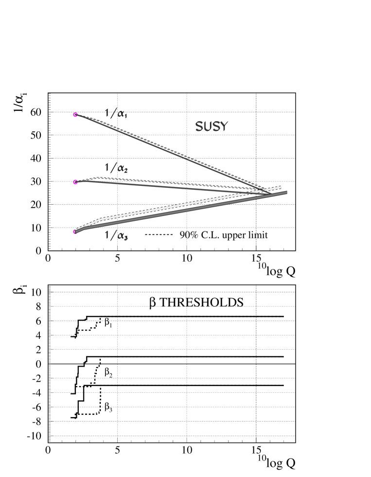
Figure 1: Evolution of the inverse of the three couplings in the MSSM. The line above $M_{\rm GUT}$ follows the prediction from the supersymmetric SU(5) model. The SUSY thresholds have been indicated in the lower part of the curve: they are treated as step functions in the first order $\beta$ coefficients in the renormalisation group equations, which correspond to a change in slope in the evolution of the couplings in the top figure. The dashed lines correspond to the 90% C.L. upper limit for the SUSY thresholds.

The upper part of Fig. 1 shows the evolution of the coupling constants in the MSSM for two cases: one for the minimum value of the $\chi^{2}$ function as defined above (solid lines) and one corresponding to the 90% C.L. upper limit of the thresholds of the light SUSY particles (dashed lines). The light thresholds are indicated in the lower function as the change in the first order coefficient in the $\beta$ function, which corresponds to the first order change in the slopes of the curves at the top. One observes that the change in $\alpha_{3}$ occurs in a rather narrow energy regime, corresponding to the threshold of squarks and gluinos, while for the other coupling constants the sleptons, higgsinos and winos contribute in addition, thus causing a somewhat more smeared threshold region.

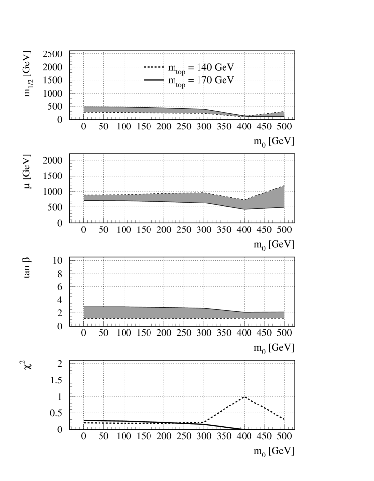
Figure 2: The fitted MSSM parameters as function of the choice of ${m_{0}}$: above ${m_{1/2}}$, middle $\mu$ and below ${\tan\beta}$. The shaded area indicates the variation, if ${m_{t}}$ is varied between 140 and 170 GeV.

The parameters corresponding to these fits are tabulated in Table 1. The initial choices of ${m_{0}}$ as well as the fitted paramters are shown at the bottom. As mentioned before, varying $A_{0}$ between $+{m_{0}}$ and $-{m_{0}}$ does not influence the results very much, so it was kept at 0, but the large radiative corrections to it were taken into account. The remaining parameters do not depend strongly on the initial choices of $m_{0}$  and $m_{t}$ , as shown in Fig. 2. The value of ${m_{0}}$ was varied between 0 and 500 GeV and ${m_{t}}$ between 140 and 170 GeV. Larger values of ${m_{0}}$ are not allowed by the dark matter constraint and the range of ${m_{t}}$ is the preferred range from the b-quark mass, as shown in Fig. 3. The difference between the two bent lines originates from the difference in $\alpha_{GUT}$ and $M_{GUT}$, as found from the fits for different input values of $m_{t}$. The horizontal band corresponds to the mass of the b-quark after QCD corrections: ${m_{b}}=4.25\pm 0.1$ GeV[30]. Although the error of 0.1 GeV is the quoted one, we used the more conservative error estimate of 0.3 GeV, since the value of the mass depends on the value of the strong coupling constant at this mass, which is not too well known. Note that the allowed range of $m_{t}$  is in excellent agreement with LEP results too[18].

In order to obtain 90% C.L. upper limits on the parameters, we varied them until the $\chi^{2}$ value increased to 1.64. Of course, this depends on the errors, so we used the rather conservative errors defined above. The upper limit on ${\tan\beta}$ was found to be about 5; here the main constraint is coming from the proton lifetime.

Since $m_{0}$  is rather small, the solutions are not strongly dependent on it, but they are mainly determined by $\mu$ and ${m_{1/2}}$. Since also ${\tan\beta}$ is constrained to a rather narrow range, we are left effectively with two parameters, $m_{1/2}$  and $\mu$. However, they were found to be strongly correlated, as shown if Fig. 4. In the minimum the $\chi^{2}$ value is zero, but one notices a long valley, where the $\chi^{2}$ is only slowly increasing. One can easily understand such a behaviour from Fig. 1: as long as the breakpoints in all curves move up simultaneously, unification can be obtained at a higher value of ${\alpha_{GUT}}$, as is obvious from a comparison of the dashed and solid lines. If one tries to combine the solid lines with the dashed lines into a single unification point, this clearly does not work. Consequently the breakpoints in all curves have to be close together in energy. However, $\alpha_{3}$ is independent of $\mu$ in contrast to the breakpoints in $\alpha_{1}$ and $\alpha_{2}$. This implies that both $\mu$ and ${m_{1/2}}$ have to increase simultaneously in order to keep the breakpoints in all three curves close together. This strong correlation has been neglected in previous analysis, where $\mu$ and ${m_{1/2}}$ were choosen independently[10][31]. This clearly cannot work in a more detailed analysis, as observed too in Ref. [32].

The steep walls in Fig. 4 originate from the experimental lower limits on the SUSY masses and the value of $M_{Z}$  from radiative symmetry breaking.

Fig. 5 shows the evolution of the masses for the minimum value of $\chi^{2}$ and ${m_{0}}$=500 GeV. From Table 1 one observes that some SUSY masses can go up to several TeV, if one considers the 90% C.L. Such large values spoil the cancellation of the quadratic divergencies. If supersymmetry would be exact, i.e. as long as the masses and couplings of the particles and their superpartners are the same, the contributions of fermions and bosons in the loops would exactly cancel each other, thus eliminating in first order all divergencies. This can be seen explicitly in the corrections to ${M_{Z}}$: $\Delta_{Z}$ is exactly zero if the masses of stop– and top quarks are identical. For the SUSY masses at the minimum value of $\chi^{2}$ the corrections to ${M_{Z}}$ are indeed very small, as shown in Fig. 6 on the left hand side, but for the solutions corresponding to the 90% C.L. upper limit the corrections to ${M_{Z}}$ are about 50 times ${M_{Z}}$ itself (see Fig. 6 right hand side). In addition, the value of the determinant^1/4=$(m_{1}^{2}m_{2}^{2}-m_{3}^{4})^{1/4}$ in the Higgs potential times its sign is shown as a dotted line. It clearly becomes negative, which implies the potential takes the shape of the mexican hat. The evolution of the masses in the Higgs potential is shown in the lower parts of Fig. 6.

If we require that only solutions are allowed, for which the corrections to ${M_{Z}}$ are not large compared with ${M_{Z}}$ itself, we have to limit the mass of the heaviest stop quark to about 1 TeV. In this case the 90% C.L. upper limits if the individual SUSY particles are given in the right hand column if Table 1. The correction to ${M_{Z}}$ = 5 times $M_{Z}$  in this case.

To determine the lower limits is somewhat more cumbersome, since not all particles reach their minimum for the same set of parameters. We used the following strategy: each parameter was scanned for the lowest possible value, while keeping the other parameters free. A zero value for the scalar mass ${m_{0}}$ could not be excluded, which corresponds to the so-called no-scale model and the corresponding results have been given in the left column of Table 1. The parameters $\mu$ and ${m_{1/2}}$ cannot be choosen independently and their minimal values were obtained for ${m_{0}}=400$ GeV, as shown in the second column of Table 1. Lower values would cause a wino mass below the experimental lower limit of about 45 GeV. The top mass for these minima was kept at 170 GeV, since smaller values would give a too high value of $m_{b}$.

One observes from Table 1 the well known effect[28]that the Higgs particle, which gets a negative mass squared before spontaneous symmetry breaking (SSB), gets only a small mass after SSB. The mass of this particle, called $h$ in Table 1, is a rather strong function of $m_{t}$, as shown in Fig. 7. For each value of $m_{t}$, the parameters ${m_{1/2}}$, $\mu$, and ${\tan\beta}$ were determined by minimising the $\chi^{2}$ for the indicated value of $m_{0}$. One observes that the mass of the lightest Higgs particle varies between 60 and 120 GeV. These values correspond to the minimal value of $\chi^{2}$, but even if the 90% C.L. limits are taken, the mass increases only to 125 GeV.

4. Summary

The MSSM model has many predictions, which can be compared with experiment, even in the energy range where the predicted SUSY particles are out of reach. Among these predictions:

• $M_{Z}$.

• $m_{b}$.

• Proton decay.

• Dark Matter.

• Upper limit on $m_{t}$.

It is surprising, that the minimal supersymmetric model can fulfil all experimental constraints for these predictions. As far as we know, supersymmetric models are the only ones, which are consistent with all these observations simultaneously. Other models can yield unification too[6], but they do not exhibit the elegant symmetry properties of supersymmetry, they offer no explanation for dark matter and no explanation for the electroweak symmetry breaking. Furthermore the quadratic divergencies do not cancel.

From the above constraints we find at the 90% C.L. (see Table 1):

$$0~{}< ~{}{m_{0}}~{} <~{}500~{}\mbox{GeV}$$

$$70~{}< ~{}{m_{1/2}}~{} <~{}3410~{}(475)~{}\mbox{GeV}$$

$$500~{}< ~{}\mu~{} <~{}3150~{}(1000)~{}\mbox{GeV}$$

$$1~{}< ~{}{\tan\beta}~{} <~{}5$$

$$138~{}< ~{}{m_{t}}~{} <~{}186~{}\mbox{GeV}$$

$$0.108~{}< ~{}{\alpha_{s}}~{} <~{}0.132$$

The upper limit on ${m_{0}}$ originates from the dark matter constraint, the upper limit on ${\tan\beta}$ from the lower limit on the proton lifetime. The fact that ${\tan\beta}$ is so much smaller than the ratio of top– and b-quark mass implies that the Yukawa coupling of the b-quark is negligibly small, so one does not have to consider its contributions in the renormalisation group equations.

Good fits are only obtained for ${\alpha_{s}}$ between 0.108 and 0.132, if the error on ${\alpha_{s}}$ is taken to be 0.008. The bottom mass constraint together with the given couplings require the top mass to be between 138 and 186 GeV.

The values in brackets indicate the 90% C.L., if one requires that the exact one-loop corrections to $M_{Z}$ are not large compared with $M_{Z}$ itself, which requires the heaviest stop quark to be below 1000 GeV. In this case the correction to $M_{Z}$  is about 5 $M_{Z}$and the corresponding constraints on the other SUSY masses are (see Table 1 for details):

$$25~{}< \tilde{\gamma}(\chi^{0}_{1}) <~{}200~{}\mbox{GeV}$$

$$45~{}< \tilde{Z}(\chi^{0}_{2}),\tilde{W}(\chi^{\pm}_{1}) <~{}385~{}\mbox{GeV}$$

$$190~{}< \tilde{g} <~{}1110~{}\mbox{GeV}$$

$$430~{}< \tilde{q} <~{}1075~{}\mbox{GeV}$$

$$200~{}< \tilde{t}_{1} <~{}730~{}\mbox{GeV}$$

$$390~{}< \tilde{t}_{2} <~{}1000~{}\mbox{GeV}$$

$$235~{}< \tilde{e}_{L} <~{}520~{}\mbox{GeV}$$

$$130~{}< \tilde{e}_{R} <~{}440~{}\mbox{GeV}$$

$$335~{}< \tilde{H} <~{}785~{}\mbox{GeV}$$

$$525~{}< {H} <~{}870~{}\mbox{GeV}$$

$$60~{}< {h} <~{}125~{}\mbox{GeV}$$

The values of ${m_{1/2}}$ and $\mu$ are positively correlated, i.e. a large (small) value of ${m_{1/2}}$ corresponds to a large (small) value of $\mu$, as is apparent from Fig. 4. This strong correlation was usually not taken into account in previous analysis, in which ${m_{1/2}}$ and $\mu$ were restricted by ad-hoc assumptions[10][31].

The detailed mass spectra have been given in Table 1. The lightest Higgs particle is certainly within reach of experiments at present or future accelerators. Its observation in the predicted mass range of 60 to 125 GeV would be a strong case in support of this minimal version of the supersymmetric grand unified theory.

Acknowledgments We thank Ugo Amaldi, Hermann Fürstenau, Stavros Katsanevas, Sergey Kovalenko, R.G. Roberts and F. Zwirner for their interest in this work and helpful discussions.

	masses in $[$GeV$]$
particles	Lower limit		best fit	Upper limit 90% C.L.
fine tuning	no	no	no	no	$m_{\tilde{t}}<1$ TeV
$\tilde{\gamma}(\chi^{0}_{1})$	134	23	46	1501	199
$\tilde{Z}(\chi^{0}_{2})$	254	46	88	2850	383
$\tilde{W}(\chi^{\pm}_{1})$	254	44	87	2900	385
$\tilde{g}$	799	193	330	6826	1109
$\tilde{e}_{L}$	236	406	412	2331	521
$\tilde{e}_{R}$	131	402	404	1384	441
$\tilde{\nu}_{L}$	228	399	406	2331	516
$\tilde{q}_{L}$	725	434	497	6035	1075
$\tilde{q}_{R}$	697	431	490	5700	1036
$\tilde{t}_{1}$	498	201	226	4740	729
$\tilde{t}_{2}$	748	391	472	5600	1000
$\tilde{H}_{1}(\chi^{0}_{3})$	550	321	417	3311	771
$\tilde{H}_{2}(\chi^{0}_{4})$	572	337	436	3323	784
$\tilde{H}^{\pm}(\chi^{\pm}_{2})$	569	337	433	3324	783
$h$	91	101	96	115	127
$H$	624	525	636	2897	871
$A$	619	523	633	2897	870
$H^{\pm}$	625	529	638	2897	873
SUSY parameters
$m_{0}$	0	400	400	500	400
$m_{1/2}$	329	70	172	3413	475
$\mu$	550	507	576	3150	1009
$\tan\beta$	2.0	3.7	2.2	2.9	3.5
$m_{t}$	147	186	172	138	175
1/$\alpha_{GUT}$	24.7	24.2	24.3	26.4	25.1
$M_{GUT}$	$1.3\;10^{16}$	$2.0\;10^{16}$	${\bf 1.9\;10^{16}}$	$0.7\;10^{16}$	$1.2\;10^{16}$

Table 1: Values of SUSY masses and parameters. For the lower limits of the SUSY masses one should take the lowest value from the first two columns, except for the value of the lightest Higgs $h$. In that case the lowest value is given by Fig. 7.

References

[1] A.D. Sakharov, ZhETF Pis’ma 5 (1967) 32

[2] The early Universe by G. Börner, Springer Verlag (1991)
The early Universe by E.W. Kolb and M.S. Turner, Addison-Wesley(1990)
A. Guth and P. Steinhardt in The new Physics, edited by P. Davis, Cambridge University Press (1989), p34.

[3] P. Fayet, Phys. Lett. B64 (1976) 159; ibid. B60 (1977) 489;
S. Dimopoulos, H. Georgi, Nucl. Phys. B193 (1981) 150;
L. E. Ibáñez, G. G. Ross, Phys. Lett. B105 (1981) 435;
S. Dimopoulos, S. Raby, F. Wilczek, Phys. Rev. D24 (1981) 1681.

[4] J. Ellis, S. Kelley, D. V. Nanopoulos, Phys. Lett. B260 (1991) 131.

[5] U. Amaldi, W. de Boer, H. Fürstenau, Phys. Lett. B260 (1991) 447.

[6] U. Amaldi et al., Phys. Lett. B281 (1992) 374.

[7] P. Langacker, M. Luo, Phys. Rev. D44 (1991) 817.

[8] J. Ellis, S. Kelley, D. V. Nanopoulos, Nucl. Phys. B373 (1992) 55

[9] Yu.A. Gol’fand, E.P. Likhtman, JETP Lett. 13 (1971) 323;
D.V. Volkov, V.P. Akulow, Phys. Lett. 46b (1971) 323;
J. Wess, B. Zumino, Nucl. Phys. B70 (1974) 39;
For further references see the review papers:
H.-P. Nilles, Phys. Rep. 110 (1984) 1;
H.E. Haber, G.L. Kane, Phys. Rep. 117 (1985) 75;
A.B. Lahanas and D.V. Nanopoulos, Phys. Rep. 145 (1987) 1;
R. Barbieri, Riv Nuo. Cim. 11 (1988) 1.

[10] G.G. Ross and R.G. Roberts, Nucl. Phys. B377 (1992) 571

[11] L. E. Ibáñez, G. G. Ross, Nucl. Phys. B368 (1992) 3 and references therein

[12] L. E. Ibáñez and C. López, Phys. Lett. 126B (1983) 54; Nucl. Phys. B233 (1984) 511

[13] P. Langacker, N. Polonski, Univ. of Pennsylvania Preprint UPR-0556-T, (1993)

[14] Arnowitt and Nath, Phys. Rev. Lett. 69 (1992) 725;
Phys. Lett. B287 (1992) 89; Phys. Lett. B289 (1992) 368; CTP-TAMU-39/92 (1992), and references therein

[15] J.L. Lopez, D.V. Nanopoulos, and H. Pois, Phys. Rev. D47 (1993) 2468.

[16] G.G. Roberts and Roszkowski, RAL-93-003

[17] Contributions from the LEP Coll. at the XXVI International Conference on High Energy Physics, Dallas, August 1992.

[18] H. Georgi, S. L. Glashow, Phys. Rev. Lett. 32 (1974) 438
H. Georgi, H. R. Quinn, S. Weinberg, Phys. Rev. Lett. 33 (1974) 451.

[19] W. A. Bardeen, A. Buras, D. Duke, T. Muta, Phys. Rev. D18 (1978) 3998.

[20] G. Degrassi, S. Fanchiotti, A. Sirlin, Nucl. Phys. B351 (1991) 49.

[21] R. Tanaka and G. Rolandi, Invited talks at the XXVI International Conference on High Energy Physics, Dallas, August 1992.

[22] T. Hebbeker, Phys. Rep. 217 (1992) 69;
S. Bethke, Plenary talk at the XXVI International Conf. on High Energy Physics, Dallas (USA), August 1992, Heidelberg Preprint HD/PY 92-13
G. Altarelli, Plenary talk at the Conf. ”QCD-20 Years later”, Aachen, Germany June 1992, CERN-TH.6623/92

[23] I. Antoniadis, C. Kounnas, K. Tamvakis, Phys. Lett. 119B (1982) 377.

[24] J. Ellis, G. Ridolfi, F. Zwirner, Phys. Lett. B262 (1991) 477
H.E. Haber R. Hempfling, Phys. Rev. Lett. 66 (1991) 83;
J. R. Espinosa, M. Quiros, Phys. Lett. B266 (1991) 389; Z. Kunszt and F. Zwirner, Nucl. Phys. B 385 (1992) 3

[25] W. de Boer, R. Ehret and D.I. Kazakov, to be published

[26] J. Gasser and H. Leutwyler, Phys. Rep. 87C (1982) 77;
S. Narison, Phys. Lett. B216 (1989) 191

[27] F. Anselmo, L. Cifarelli, A. Peterman, A. Zichichi, Il Nuovo Cimento 105 (1992) 1179

[28] M. Carena, S. Pokoroski, C.E.M. Wagner, Max-Planck-Institute Preprint MPI-PH-93-10 (1993), and private communication

Figure 3: The correlation between ${m_{b}}$ and ${m_{t}}$ for ${m_{0}}=500$ GeV. The hatched area indicates the experimental value for ${m_{b}}=4.25\pm 0.3$ GeV (the crossed area for ${m_{b}}=4.25\pm 0.1$ GeV) and the curved lines give the correlation for different values of the coupling constant at the GUT scale.

Figure 4: The correlation between ${m_{1/2}}$ and $\mu$ for ${m_{0}}$=500 GeV. The vertical axis gives the value of $\chi^{2}$.

Figure 5: The evolution of masses of the SUSY particles. The lines indicated as photino and zino are the lines corresponding to the two lightest neutralinos, while the lines of wino and charged higgsino correspond to the two lightest charginos. The lightest Higgs (neutral Higgs 2 in lower left corner) gets its small mass only after spontaneous symmetry breaking via the Higgs mechanism.

Figure 6: The evolution of the $M_{Z}$ mass, the determinant in the Higgs potential, and the value of the Higgs mass squared for the optimum solution (left) and the solution corresponding to the 90% C.L. upper limits (right). The dashed lines in the top curves show the solution of the minimization of the Higgs potential at the tree level. This line coincides with the solid line for the best solution, as expected if supersymmetry is not badly broken, but the one-loop corrections to the $M_{Z}$  masses become unnaturally large for the right hand side.

Figure 7: The mass of the lightest Higgs particle as function of the top quark mass. The parameters of $\tan\beta$, $m_{0}$, and $m_{1/2}$ were optimised for each choice of $m_{t}$ and $m_{0}$.