8.5in 11.0in 1.0in 1.0in 0.5in 1.8in 1.0in

UCLA/93/TEP/26
July 1993
(Bulletin Board : hep-ph/9307369)

Observing $b\rightarrow s\,\mu^{+}\mu^{-}$ Decays at Hadron Colliders
Grant Baillie
Department of Physics
University of California, Los Angeles
405 Hilgard Avenue
Los Angeles, CA 90024–1547
(E-mail : baillie@physics.ucla.edu)
Abstract
We examine the prospects for observing weak flavour-changing neutral current (FCNC) decays of $B$ mesons at hadron colliders, including effects of anomalous $WWZ$ vertices. Since it is very difficult to measure the inclusive rate $B\rightarrow X_{s}\,\mbox{$\ell^{+}$}\mbox{$\ell^{-}$}$ one should consider exclusive modes such as $B\rightarrow\mbox{$K^{*}$}\,\mbox{$\mu^{+}$}\mbox{$\mu^{-}$}$ and $B\rightarrow K\,\mbox{$\mu^{+}$}\mbox{$\mu^{-}$}$. Even though this requires one to compute hadronic matrix elements, we show that experimentally observable quantities (ratios of decay rates) are not strongly parametrisation dependent. Some possibilities for reducing the theoretical uncertainties from other experimental data are discussed.

1 Introduction

Because weak flavour-changing neutral currents (FCNC’s) are forbidden at tree level in the Standard Model Lagrangian, transitions involving these currents are potentially sensitive tests of electroweak radiative corrections. Beside their dependence on the as yet undetermined top quark mass $m_{t}$, FCNC processes could provide a clear signal for “new physics”, stemming from the presence of non-Standard Model particles or couplings in loop graphs. For example, contributions to the decays $b\rightarrow s\gamma$ and $b\rightarrow s\,\mbox{$\ell^{+}$}\mbox{$\ell^{-}$}$ have been calculated in the context of supersymmetry [1], two-Higgs models [1, 2], anomalous $WW\gamma$ couplings [3] and heavy fermions [4].

Recently the CLEO collaboration, observing $e^{+}e^{-}$ annihilation at the $\Upsilon(4S)$ resonance, has detected the decay $B\rightarrow\mbox{$K^{*}$}\gamma$ [5]; in addition an upper bound on the branching fraction $B(\mbox{$b\rightarrow s\gamma$})$ has been claimed [6]. These results already provide interesting bounds on non-Standard Model physics, which will be constrained further once the top quark is discovered [7]. For $b\rightarrow s\,\mbox{$\mu^{+}$}\mbox{$\mu^{-}$}$, the UA1 collaboration has determined the experimental upper bound to be $B(\mbox{$b\rightarrow s\,\mbox{$\mu^{+}$}\mbox{$\mu^{-}$}$})<5.0\times 10^{-5}$, leaving room for substantial deviation from the standard model prediction $(6-8)\times 10^{-6}$ [8]. Because of the large production cross-section for heavy quarks at hadron colliders, an observation of these decays may be possible by the D0 and CDF experiments, which have recently completed data collection runs of proton-antiproton collisions at $\sqrt{s}=1800$ GeV. It is therefore important to make theoretical predictions for these rare decays that take into account some of the experimental difficulties associated with measuring them at hadron machines.

The rate for $b\rightarrow s\,\mbox{$\ell^{+}$}\mbox{$\ell^{-}$}$ can be computed quite straightforwardly once a low-energy effective Lagrangian has been obtained by “integrating out” heavy degrees of freedom. Unfortunately, at hadron colliders it is difficult to measure the corresponding inclusive branching ratio $B(B\rightarrow X_{s}\mbox{$\ell^{+}$}\mbox{$\ell^{-}$})$, where $X_{s}$ denotes a final state containing a strange (but not charm) quark. Because of the large number of final state hadrons produced in any single event, identifying a subset of particles as originating from a $B$ involves reconstructing their total 4-momentum and invariant mass. The presence of multiparticle states in the inclusive sum then makes it hard to disentangle $B$ decay events from the general hadronic background. Consequently, one is led to consider particular (or “exclusive”) decay modes, such as $B\rightarrow\mbox{$K^{*}$}(892)\mbox{$\ell^{+}$}\mbox{$\ell^{-}$}$ or $B\rightarrow K\,\mbox{$\ell^{+}$}\mbox{$\ell^{-}$}$. This is unpleasant from the theorist’s point of view, because one now needs to know the matrix elements of quark operators between hadronic final states. At present, these cannot be computed from first principles (i.e. from QCD), and various models and approximations have to be used to estimate them. We will make a case for using some of the results of heavy quark effective theory for the form factors here, even though the $s$ quark cannot really be considered heavy. We will estimate model-dependence by considering several different expressions for the Isgur-Wise function, which parametrises the form factors.

For simplicity we choose to investigate only decay channels involving a pair of muons. This is motivated partially by the fact that present detectors at hadron colliders are more efficient at detecting muon pairs than electron pairs in this energy regime. In addition, we note that the low-dimuon mass region is very difficult to study experimentally, in part because the muons tend to be less separated there, and also because of backgrounds (typically, some kind of cut has to be imposed on muon transverse momentum — see ref. [9], for example).

We therefore consider the decays $B\rightarrow\mbox{$K^{*}$}\,\mbox{$\mu^{+}$}\mbox{$\mu^{-}$}$ and $B\rightarrow K\,\mbox{$\mu^{+}$}\mbox{$\mu^{-}$}$with dimuon invariant mass above the $\psi$ peak in what follows. In Section 2, we briefly review the amplitude for $b\rightarrow s\,\mbox{$\ell^{+}$}\mbox{$\ell^{-}$}$ processes in the Standard Model, taking into account QCD corrections and the contribution of $c\bar{c}$ pairs. After some discussion on estimating hadronic matrix elements, we make some predictions within the Standard Model. As an example of how these predictions are affected by “new physics”, in particular new physics that cannot be constrained by $b\rightarrow s\gamma$ decays, we consider the effect of non-Standard Model $WWZ$ couplings in Section 4. The results will be discussed in Section 5, and finally, we draw conclusions in Section 6.

2 The process $b\rightarrow s\,\mbox{$\ell^{+}$}\mbox{$\ell^{-}$}$

The amplitude for the decay $b\rightarrow s\,\mbox{$\ell^{+}$}\mbox{$\ell^{-}$}$ can be written in the form

$${\cal M}={4G_{F}\over\sqrt{2}}{\alpha(m_{b})\over 4\pi x_{\scriptstyle W}}V^{*}_{ts}V_{tb}\left\{A\>\bar{s}\gamma^{\mu}Lb\>\bar{\ell}\gamma_{\mu}L\ell+B\>\bar{s}\gamma^{\mu}Lb\>\bar{\ell}\gamma_{\mu}R\ell+x_{W}F\>{i\over q^{2}}m_{b}\,\bar{s}\mbox{$\sigma^{\mu\nu}$}q_{\nu}Rb\>\bar{\ell}\gamma_{\mu}\ell\right\},$$ (1)

where $\alpha(m_{b})\approx 1/132.7$ is the QED running coupling evaluated at the $b$ scale, $G_{F}$ is the Fermi weak decay constant, $x_{W}=\sin^{2}\theta_{W}$ ($\theta_{W}$ is the Weinberg angle), $V$ is the Kobayashi-Maskawa (KM) matrix, $s$ and $b$ are quark spinors and $R$ and $L$ are the projection operators $(1+\gamma^{5})/2$ and $(1-\gamma^{5})/2$, respectively. We have defined $q^{\mu}$ to be the total outgoing 4-momentum of the final $\ell^{+}$$\ell^{-}$ pair in the decay $b\rightarrow s\,\mbox{$\ell^{+}$}\mbox{$\ell^{-}$}$. In addition, in the $F$ term, a contribution proportional to $m_{s}$ has been dropped. Throughout, we use the conventions $\sigma_{\mu\nu}=i/2\left[\gamma_{\mu},\gamma_{\nu}\right]$ and $\epsilon_{0123}=+1$.

In an effective field theory approach, $A$, $B$ and $F$ arise from the graphs of figure 1. (Note that the contribution of $u$-quark graphs is KM suppressed; we make the usual approximation $V^{*}_{ts}V_{tb}\approx-V^{*}_{cs}V_{cb}$, $V^{*}_{us}V_{ub}\approx 0$.) The $\bar{s}b\,\bar{\ell}\ell$ terms of figure 1(a) appear in the low-energy effective Lagrangian as a result of integrating out $Z$ exchange and $W$ box diagrams at $\mu\sim M_{W}$. Also, $\bar{s}b\gamma$ vertices contribute via figure 1(b). In particular, the $1/q^{2}$ pole in front of the $F$ term above is a result of there being an on-shell photon intermediate state at $q^{2}=0$ (the coefficient $F$ also appears in the rate for $b\rightarrow s\gamma$). Finally, the sum of the two graphs represented by figure 1(c) can be evaluated as in ref. [12], where the charm loop is expressed as a dispersion integral which receives continuum (essentially free quark) and $c\bar{c}$ resonance contributions. The latter, because of the narrow widths involved, amount to adding Breit-Wigner terms for the $\psi\,(3097)$ and $\mbox{$\psi^{\prime}$}\,(3685)$ to both $A$ and $B$:

$$A\>(B)\quad\rightarrow\quad A\>(B)+(C_{9}+3C_{10})\,{3\pi x_{W}\over\alpha^{2}(m_{b})}\,{M_{\psi}\Gamma(\mbox{$\psi\rightarrow\mbox{$\ell^{+}$}\mbox{$\ell^{-}$}$})\over q^{2}-M_{\psi}^{2}+iM_{\psi}\Gamma_{\psi}}\>+\>(\psi\rightarrow\psi^{\prime})$$ (2)

where

$$C_{9}+3C_{10}=2\left\{\alpha_{s}\,(m_{b})/\alpha_{s}\,(M_{W})\right\}^{-6/23}-\left\{\alpha_{s}\,(m_{b})/\alpha_{s}\,(M_{W})\right\}^{12/23}$$ (3)

is a QCD-corrected Wilson coefficient evaluated at the $b$ scale. In general, then, the coefficients $A$, $B$ and $F$ depend on $x_{t}\equiv m_{t}^{2}/M_{W}^{2}$ (a result of integrating out heavy degrees of freedom at the $W$ scale), and also contain QCD correction terms (computed by running Wilson coefficients in the effective Lagrangian down from $\mu=M_{W}$ to $\mu=m_{b}$) and both short- and long-distance contributions from charm loops. Explicit expressions can be found in ref. [10]; detailed calculations are to be found in the references therein. In terms of their coefficient functions $A_{1,2,3}$ of [10] we have

$$A = x_{W}(A_{1}+A_{3})$$ (4)

$$B = x_{W}A_{1}$$ (5)

$$F = -2A_{2}$$ (6)

We also note that, for values of the top quark mass in the range 100–200 GeV, the coefficient $A$ (excluding the charm contributions) is a good deal larger than $B$ or $x_{W}F$. For example, at $m_{t}=150$ GeV we find $A=1.58$, $B=-0.0737$ and $x_{W}F=0.144$ when $\Lambda_{\rm QCD}^{(4)}=150$ MeV.

3 Exclusive rare $B$ decays

To compute the rates for $B\rightarrow\mbox{$K^{*}$}\,\mbox{$\mu^{+}$}\mbox{$\mu^{-}$}$ and $B\rightarrow K\,\mbox{$\mu^{+}$}\mbox{$\mu^{-}$}$ in the spectator quark approximation, one needs to know the matrix elements of $\bar{s}\gamma^{\mu}Lb$ and $\bar{s}i\mbox{$\sigma^{\mu\nu}$}q_{\nu}Rb$ sandwiched between the initial and final hadronic states. In this paper, we assume that these matrix elements have the form prescribed by heavy quark effective theory (HQET) [11]:

$$\begin{array}[]{rcl}\displaystyle\left\langle K(v^{\prime})\right|\bar{s}\gamma^{\mu}Lb\left|B(v)\right\rangle&=&\displaystyle-{1\over 2}\sqrt{M_{B}M_{K}}\;\mbox{$\xi\left(v\cdot v^{\prime}\right)$}\;\left(v+v^{\prime}\right)^{\mu}\\[10.0pt] \displaystyle\left\langle K(v^{\prime})\right|\bar{s}i\mbox{$\sigma^{\mu\nu}$}q_{\nu}Rb\left|B(v)\right\rangle&=&\displaystyle-{1\over 2}\sqrt{M_{B}M_{K}}\;\mbox{$\xi\left(v\cdot v^{\prime}\right)$}\;\left(v^{\prime\mu}v^{\nu}-v^{\mu}v^{\prime\nu}\right)q_{\nu}\end{array}$$ (7)

and

$$\begin{array}[]{rcl}\displaystyle\left\langle\mbox{$K^{*}$}(v^{\prime},\epsilon)\right|\bar{s}\gamma^{\mu}Lb\left|B(v)\right\rangle&=&\displaystyle{1\over 2}\sqrt{M_{B}M_{K^{*}}}\;\mbox{$\xi\left(v\cdot v^{\prime}\right)$}\;\times\\[10.0pt] &&\quad\displaystyle\left(i\epsilon^{\mu\alpha\beta\gamma}\;\epsilon^{*}_{\alpha}\;v_{\beta}\;v^{\prime}_{\gamma}+(1+v\cdot v^{\prime})\;\epsilon^{*\mu}-v\cdot\epsilon^{*}\;v^{\prime\mu}\right)\\[10.0pt] \displaystyle\left\langle K^{*}(v^{\prime})\right|\bar{s}i\mbox{$\sigma^{\mu\nu}$}q_{\nu}Rb\left|B(v)\right\rangle&=&\displaystyle{1\over 2}\sqrt{M_{B}M_{K^{*}}}\;\mbox{$\xi\left(v\cdot v^{\prime}\right)$}\;\times\\[10.0pt] &&\quad\displaystyle\left(i\epsilon^{\mu\nu\alpha\beta}\;\epsilon^{*}_{\alpha}\;(v+v^{\prime})_{\beta}+(v+v^{\prime})^{\mu}\epsilon^{*\nu}-(v+v^{\prime})^{\nu}\epsilon^{*\mu}\right)q_{\nu}.\end{array}$$ (8)

Here $\epsilon$ is the $K^{*}$ polarisation vector, $v$ and $v^{\prime}$ are the $B$ and $K^{(*)}$ 4-velocities (so that 4-momenta are given by $p_{B}^{\mu}=M_{B}v^{\mu}$, $p_{K^{(*)}}^{\mu}=M_{K^{(*)}}v^{\prime\mu}$) and $\xi\left(v\cdot v^{\prime}\right)$ is the Isgur-Wise function. Strictly speaking, the 4-vector $q^{\mu}$ is the difference between the $b$ quark and $s$ quark momenta, but we make the usual identification $q^{\mu}=p_{B}^{\mu}-p_{K^{(*)}}^{\mu}$.

Of course, one should be suspicious of using the heavy quark method in this case, because corrections to its predictions are expected to be of order $\mbox{$\Lambda_{\rm QCD}$}/m_{Q}$, which is not a particularly small number for the strange quark. In the $K^{*}$ case, a general Lorentz-invariant decomposition of the left-hand sides of equation (8) would involve seven different functions of $q^{2}$, which all turn out to be related to the Isgur-Wise function $\xi\left(v\cdot v^{\prime}\right)$ by the heavy quark symmetry when $\>m_{s}\;,\;m_{b}\gg\mbox{$\Lambda_{\rm QCD}$}$. In spite of the fact that $\>m_{s}\not\gg\mbox{$\Lambda_{\rm QCD}$}$, it is shown in refs. [13, 14] that these relations amongst form factors coninue to hold to about 10%, mainly as a result of the heaviness of the $b$ quark, and also the fact that the $K^{*}$ meson is in some sense “weakly bound”.

Note that one can test some of the heavy-quark relations amongst $\bar{s}\gamma^{\mu}Lb$ form factors by measuring the polarisation of the $K^{*}$ meson in the decays $B\rightarrow K^{*}\,\psi$and $B\rightarrow K^{*}\,\psi^{\prime}$. Even though this leaves open the possibility of deviations in the remaining $\bar{s}\mbox{$\sigma^{\mu\nu}$}b$ matrix elements, the two sets of form factors can be related by the plausible assumption that the $b$ quark is static within the $B$ meson [13].

The $K$ meson, on the other hand, is a relativistic bound state, and it might not be appropriate to apply the constituent quark model analysis of [13, 14] here. Nevertheless, if one performs a general decomposition of the matrix elements in equation (7), one finds that only two of the three resulting form factors contribute to $B\rightarrow K\,\mbox{$\mu^{+}$}\mbox{$\mu^{-}$}$. In addition, because $A\gg B{\rm\ or\ }x_{W}F$, one of the two will dominate this decay. (Note that there are no $q^{2}=0$ poles in the decay rate to enhance the contribution of $F$: these would be a result of an on-shell intermediate $B\rightarrow K\gamma$ transition, which is forbidden by angular momentum conservation). Consequently, deviations from the heavy quark relations amongst $K$ form factors are unlikely to have a great effect on the rate.

It should be pointed out that extending the heavy quark spin-flavour symmetry to the $s$ quark case could be dubious. In other words, one cannot assume that the function $\xi$ above is related to the function $\xi$ determined from $b$ and $c$ decays (flavour symmetry); nor can one really say that the functions $\xi$ in equations (8) and (7) are the same (spin symmetry). (However, we shall continue to refer to the two functions $\xi_{K}$ and $\xi_{K^{*}}$ generically as $\xi$, unless we need to distinguish between the two.) Essentially, we are using the heavy quark form of the matrix elements as a convenient ansatz which appears to hold to a good degree of accuracy.

Another property of HQET is that at the zero-recoil point, where $v\cdot v^{\prime}=1$, the Isgur-Wise function satisfies $\xi\;(1)=1$. We are reluctant to assume this is the case in $b\rightarrow s$ transitions — for example, one can note that $m_{s}$, $M_{K}$ and $M_{K^{*}}$ are all supposed to be degenerate in the heavy quark limit. In constituent quark models one finds that the above normalisation condition holds in the case of large quark masses. However, an explicit computation of form factors in the naïve quark model of ref. [13] gives $\xi\;(1)\approx 0.7$ in the $B\rightarrow K$ case. (This is not surprising, as $1/m_{Q}$ corrections are known to be large for pseudoscalar $\rightarrow$ pseudoscalar transitions). Consequently, we avoid issues of normalisation of our form factors by taking ratios of decay rates. This is also desirable from the experimental point of view, as some uncertainties, like luminosity and detector efficiency, then tend to cancel.

In view of our earlier comments about the difficulty of observing the small $q^{2}$ region, it makes sense to divide out the $\psi$ peak, and make predictions for the quantities

$$R^{(*)}={\displaystyle\Gamma_{1}\left(B\rightarrow K^{(*)}\mbox{$\mu^{+}$}\mbox{$\mu^{-}$}\right)\over\displaystyle\Gamma_{2}\left(B\rightarrow K^{(*)}\mbox{$\mu^{+}$}\mbox{$\mu^{-}$}\right)}$$ (9)

where $\Gamma_{1}$ is the contribution of the region of phase space with $\hat{s}\equiv q^{2}/M_{B}^{2}$ above the $\psi$ peak, with the $\psi^{\prime}$ excluded, while $\Gamma_{2}$ is the contribution of the $\psi$ peak itself. Specifically, we will assume

$$\Gamma_{1} = \left(\int_{0.35}^{0.48}\mbox{$\rm d$}\hat{s}+\int_{0.50}^{{\hat{s}}_{\rm max}}\mbox{$\rm d$}\hat{s}\right)\;{\mbox{$\rm d$}\over\mbox{$\rm d$}\hat{s}}\,\Gamma$$ (10)

$$\Gamma_{2} = \int_{0.34}^{0.35}\mbox{$\rm d$}\hat{s}{\mbox{$\rm d$}\over\mbox{$\rm d$}\hat{s}}\,\Gamma\>,$$ (11)

since ${\hat{s}}_{\psi}\approx 0.344$ and ${\hat{s}}_{\psi^{\prime}}\approx 0.487$. Here the differential decay widths can be computed from equations (1), (7) and (8):

$$\begin{array}[]{rcl}\displaystyle{\mbox{$\rm d$}\over\mbox{$\rm d$}\hat{s}}\,\Gamma\,(\mbox{$B\rightarrow K\,\mbox{$\mu^{+}$}\mbox{$\mu^{-}$}$})&=&\displaystyle{G_{F}^{2}M_{B}^{5}\over 192\pi^{3}}\,\left|V^{*}_{ts}V_{tb}\right|^{2}\,\left({\alpha(m_{b})\over 4\pi x_{W}}\right)^{2}\,2\kappa^{2}\,\xi^{2}(y)\,\left(y^{2}-1\right)^{3/2}\quad\times\\[10.0pt] &&\displaystyle\phantom{+}\left\{\vphantom{|\over|}-2\,(\kappa+1)\,F\,\mbox{\rm Re}\,(A+B)\,+(\kappa+1)^{2}\,\left(\left|A\right|^{2}+\left|B\right|^{2}\right)+2\,F^{2}\vphantom{|\over\|}\right\}\end{array}$$ (12)

and

$$\begin{array}[]{rcl}\displaystyle{\mbox{$\rm d$}\over\mbox{$\rm d$}\hat{s}}\,\Gamma\,(\mbox{$B\rightarrow\mbox{$K^{*}$}\,\mbox{$\mu^{+}$}\mbox{$\mu^{-}$}$})&=&\displaystyle{G_{F}^{2}M_{B}^{5}\over 192\pi^{3}}\,\left|V^{*}_{ts}V_{tb}\right|^{2}\,\left({\alpha(m_{b})\over 4\pi x_{W}}\right)^{2}\,2\mbox{$\kappa^{*}$}^{2}\,(1+y)\,\xi^{2}(y)\,\left(y^{2}-1\right)^{1/2}\quad\times\\[10.0pt] &&\displaystyle\phantom{+}\left\{\vphantom{|\over|}2\,F\,\mbox{\rm Re}\,(A+B)\,\left((5\mbox{$\kappa^{*}$}-1)+(\mbox{$\kappa^{*}$}-5)^{\phantom{1}}y\right)\right.\\[10.0pt] &&\displaystyle\phantom{+}\left.\,+\,{2F^{2}\over\hat{s}}\,\left((\mbox{$\kappa^{*}$}^{2}-8\mbox{$\kappa^{*}$}+1)+(5\mbox{$\kappa^{*}$}^{2}-2\mbox{$\kappa^{*}$}+5)\;y-2\mbox{$\kappa^{*}$}y^{2}\right)\right.\\[10.0pt] &&\displaystyle\phantom{+}\left.\,+\,\left(\left|A\right|^{2}+\left|B\right|^{2}\right)\,\left((\mbox{$\kappa^{*}$}-1)^{2}+(5\mbox{$\kappa^{*}$}^{2}-2\mbox{$\kappa^{*}$}+5)\;y-8\mbox{$\kappa^{*}$}y^{2}\right)\vphantom{|\over|}\right\}.\end{array}$$ (13)

We have defined $\kappa\equiv M_{K}/M_{B}$, $\mbox{$\kappa^{*}$}\equiv M_{K^{*}}/M_{B}$, and $y\equiv v\cdot v^{\prime}=1/2\left((1-\hat{s})/\kappa^{(*)}+\kappa^{(*)}\right)$.

It should be noted that $\Gamma_{2}$ is essentially proportional to the square of the QCD coefficient in equation (3). However, as pointed out in ref. [15], because of an accidental cancellation, this quantity is highly sensitive to the value of $\Lambda_{\rm QCD}$. For example, we find that, for the $K^{*}$ transition, $\Gamma_{2}$ changes by a factor of about two as $\Lambda^{(4)}_{QCD}$ varies from 150 to 300 MeV. Following [15], we will replace this coefficient in the Breit-Wigner amplitudes by its QCD-uncorrected value of 1, which gives a reasonably good agreement with the measured $B\rightarrow X\psi$ inclusive branching ratio.

Finally, we choose various parametrisations of the function $\xi$ above. First of all, we consider the simple monopole and exponential expressions

$$\xi_{I}\,(y)={w_{0}^{2}/2\over w_{0}^{2}/2-1+y}$$ (14)

$$\xi_{II}\,(y)=\exp\alpha\,(1-y),$$ (15)

taking for $\alpha$ and $w_{0}$ the values determined from $D\rightarrow K\ell\nu$ decays in [16]: $\alpha\approx 0.5$ and $w_{0}\approx 1.8$.

Also, we consider the two forms given in ref. [17]:

$$\xi_{III}\,(y)=\left({2\over y+1}\right)^{2\rho^{2}}$$ (16)

$$\xi_{IV}\,(y)={2\over y+1}\exp\left(-\beta{y-1\over y+1}\right),$$ (17)

with $\beta$ and $\rho$ computed from $B\rightarrow D^{*}\ell\nu$ to be $\beta\approx 1.84$ and $\rho\approx 1.14$.

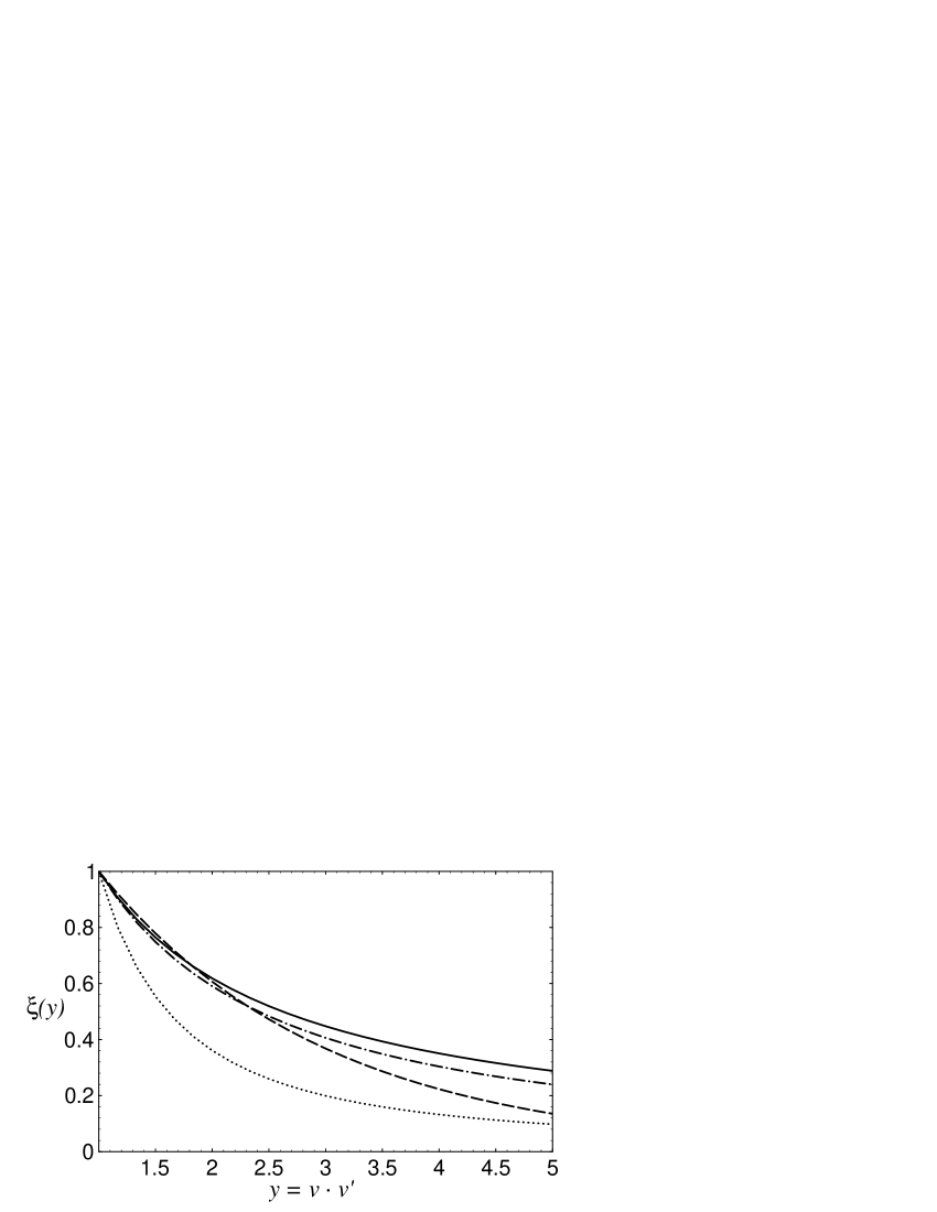
Figure 2: Plot of the four different parametrisations of the Isgur-Wise function $\xi_{i}(y)$. $i=$ I is given by solid lines, II by dashed, III by dotted and IV by dot-dashed lines. See equations (14)–(17).

The above four functions are plotted in figure 2. Although it might seem strange to use fits to both $D\rightarrow K\ell\nu$ and $B\rightarrow D^{*}\ell\nu$ decays, this at least gives some kind of idea of uncertainties due to the strange quark mass not being small. Plots of $R$ and $R^{*}$, for top quark masses between 100 and 200 GeV, are presented in figures 3 and 4. We defer discussion of these results to Section 5.

4 Effect of non-SM $WWZ$ couplings

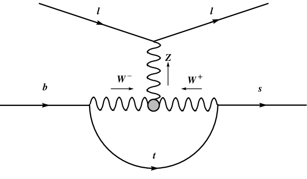
Figure 5: Contribution of anomalous $WWZ$ couplings to $b\rightarrow s\,\mbox{$\ell^{+}$}\mbox{$\ell^{-}$}$

The contribution of a non-Standard Model $WWZ$ vertex to the $b\rightarrow s\,\mbox{$\ell^{+}$}\mbox{$\ell^{-}$}$ amplitude is shown in figure 5. At a scale $\mu=M_{W}$, we can assume all external lines have zero 4-momentum. In this case, we can ignore derivatives of the $Z$ field in the anomalous vertex, so that the full Lorentz- and $U(1)$-invariant vertex of ref. [20] reduces to two terms:

$${\cal L}_{\rm WWZ}=-ie\cot\theta_{W}\;Z_{\mu}\left\{\;g_{1}^{Z}\left(W_{\nu}W^{{\dagger}\;\mu\nu}-W^{{\dagger}}_{\nu}W^{\mu\nu}\right)-ig_{5}^{Z}\epsilon^{\mu\nu\rho\sigma}W^{{\dagger}}_{\nu}\mathop{\partial_{\rho}}^{\leftrightarrow}W_{\sigma}\;\right\}$$

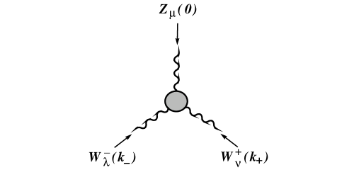
Figure 6: Definitions for the Feynman rule for the non-Standard Model part of the $WWZ$ vertex, at zero $Z$ momentum

where $W^{\mu}$ is the $W^{-}$ field, and $A\;{\displaystyle\mathop{\partial_{\rho}}^{\leftrightarrow}}\,B\equiv A\left(\partial_{\rho}B\right)-\left(\partial_{\rho}A\right)B$. In the Standard Model, $g_{1}^{Z}=1$ and $g_{5}^{Z}=0$, so the Feynman rule for the (non-SM) vertex of figure 6 is:

$$-ie\cot\theta_{W}\left\{\Delta g_{1}^{Z}\left[\left(k_{+}-k_{-}\right)^{\mu}g^{\nu\lambda}+k_{-}^{\nu}g^{\mu\lambda}-k_{+}^{\lambda}g^{\mu\nu}\right]+ig^{Z}_{5}\epsilon^{\nu\lambda\rho\mu}\left(k_{-}-k_{+}\right)_{\rho}\right\}.$$

In an effective Lagrangian formalism, we need to compute the graph of figure 5, which amounts to computing the non-Standard Model $\bar{s}bZ$ vertex at zero external momentum. Working for the moment in $R_{\xi}$ gauge, we find the $b\rightarrow sZ$ amplitude to be

$$\begin{array}[]{rl}\displaystyle{g^{3}\cos\theta_{W}\over 2}\,V^{*}_{ts}V_{tb}\,\int{\mbox{$\rm d$}^{4}k\over\left(2\pi\right)^{4}}&\displaystyle{-\bar{s}\;\gamma_{\alpha}\not k\,\gamma_{\beta}L\;b\over\left(k^{2}-M_{W}\right)^{2}}\;\left({1\over k^{2}-m_{t}^{2}}-{1\over k^{2}}\right)^{\vphantom{2}}\>D^{\beta\lambda}_{\xi}\,(k)\;D^{\alpha\nu}_{\xi}\,(k)\times\\[10.0pt] &\left(\Delta g_{1}^{Z}\left(k^{\nu}g^{\mu\lambda}-2k^{\mu}g^{\lambda\nu}+k^{\lambda}g^{\mu\nu}\right)+2ig_{5}^{Z}\epsilon^{\nu\lambda\rho\mu}k_{\rho}\right)\end{array}$$ (18)

with $D^{\alpha\beta}\,(k)=g^{\alpha\beta}-(1-\xi)k^{\alpha}k^{\beta}/(k^{2}-\xi M_{W}^{2})$. Note that here we have used GIM cancellation to subtract off the $m_{t}$-independent portion [4]. In the above, it is clear that the $g^{Z}_{5}$ contribution is gauge-independent — the longitudinal terms in the $W$ propagators don’t contribute — and finite. However, the $\Delta g^{Z}_{1}$ term does depend on $\xi$. This term should therefore be computed in the physical (unitary) gauge, obtained in the limit $\xi\rightarrow\infty$. However, in this limit the integral is logarithmically divergent. (Note that computing this graph with a Standard Model $WWZ$ vertex also gives a divergent result in unitary gauge, but gauge invariance leads to a “miraculous” cancellation between divergences in physical amplitudes.) We can regulate this divergence via the prescription

$$\xi\rightarrow\Lambda^{2}/M_{W}^{2}\gg 1,$$ (19)

with $\Lambda$ a cutoff. The integral in (18) can now be evaluated explicitly, giving

$${g^{3}\cos\theta_{W}\over 2}\,V^{*}_{ts}V_{tb}\,{i\over 16\pi^{2}}\,\bar{s}\gamma_{\mu}Lb\,\left(\Delta g_{1}^{Z}F_{1}(x_{t},\Lambda)+g_{5}^{Z}F_{5}(x_{t})\right)$$ (20)

where

$$x_{t} \equiv m_{t}^{2}/M_{W}^{2},$$ (21)

$$F_{1}(x_{t},\Lambda) = {3\over 2}x_{t}\left(\log{\displaystyle\Lambda^{2}\over M_{W}^{2}}+{1\over 1-x_{t}}+{2x_{t}-x_{t}^{2}\over\left(1-x_{t}\right)^{2}}\log x_{t}\right),$$ (22)

$$F_{5}(x_{t}) = -{3x_{t}\over 1-x_{t}}\left(1+{\displaystyle x_{t}\log x_{t}\over 1-x_{t}}\right).$$ (23)

Thus the contribution of the anomalous vertex to the amplitude of equation (1) is

$$\begin{array}[]{rl}{\cal M}=&\displaystyle{4G_{F}\over\sqrt{2}}\,{\alpha(m_{b})\over 4\pi x_{\scriptstyle W}}\,V^{*}_{ts}V_{tb}\,(1-x_{W})\,\left(\Delta g_{1}^{Z}F_{1}(x_{t},\Lambda)+g_{5}^{Z}F_{5}(x_{t})\right)\times\\ &\quad\left(-(x_{W}-{1\over 2})\,\bar{s}\gamma^{\mu}Lb\>\bar{\ell}\gamma_{\mu}L\ell-x_{W}\,\bar{s}\gamma^{\mu}Lb\>\bar{\ell}\gamma_{\mu}R\ell\right).\end{array}$$ (24)

It turns out that four-Fermi operators of the above type do not scale below $\mu=M_{W}$, because $\bar{s}\gamma^{\mu}(\gamma^{5})b$ are currents of a softly-broken symmetry. Consequently, we can ignore QCD corrections to equation (24).

In figures 7–10 we fix $m_{t}=150$ GeV and $\Lambda=1$ TeV, and plot $R$ and $R^{*}$ as functions of $\Delta g_{1}^{Z}$ and $g_{5}^{Z}$.

5 Discussion

Since we have been calculating ratios of decay rates, it isn’t clear when these processes will become observable at hadron colliders. In this regard, it is worth pointing out that, in the current Tevatron run, CDF has roughly a hundred $BKspsi$ events, so that the non-resonant $B\rightarrow\mbox{$K^{*}$}\,\mbox{$\mu^{+}$}\mbox{$\mu^{-}$}$ process is an order of magnitude beyond reach. (From figure 4, $R^{*}$ is typically of order $10^{-3}$). In addition, branching ratios involving a $K$ in the final state are typically a factor of 3–6 smaller than the corresponding $K^{*}$ processes. However, future planned runs will begin to put useful bounds on non-Standard Model physics, and clearly proposed hadron machines such as LHC or SSC will be able to shed further light on these rare decays.

As can be seen in figures 3 and 4, substantial uncertainties are present in our predictions, typically of order 25% at fixed top quark mass. These uncertainties stem mainly from not knowing the momentum dependence of the form factors; in other words, from having to extrapolate the Isgur-Wise function to larger values of $v\cdot v^{\prime}$. We would like to point out, however, that the procedure of normalising spectra to the $\psi$ peak (partially motivated by the constraints of making measurements at hadron colliders) reduces these extrapolation uncertainties considerably. This can be seen by comparing figure 2 with the various plots of $R$ and $R^{*}$, bearing in mind that probability distributions are proportional to $\xi^{2}$.

In fact, our procedure has intentionally been rather crude — for example, we have not attempted to include uncertainties in the Isgur-Wise parameters of equations (14) – (17), and consequently we have no quantitative measure of errors induced by the various parametrisations. Nevertheless, experimental data can help to reduce and quantify these errors. In particular, the long-distance $\psi$ and $\psi^{\prime}$ peaks in the dimuon spectrum, allow one to measure $B\rightarrow K^{(*)}$ form factors at the corresponding values of $q^{2}$. In our approach, where ratios of amplitudes are measured, one could use the experimentally measured value of $\Gamma(B\rightarrow K^{(*)}\psi)\,/\,\Gamma(B\rightarrow K^{(*)}\mbox{$\psi^{\prime}$})$ to fit the parameters of the Isgur-Wise function experimentally. This procedure is quite similar to that of ref. [18], except that, as mentioned before, we are avoiding using the overall normalisation of the $B\rightarrow K^{(*)}$ form factors, and are reluctant to assume that $\mbox{$K$}-\mbox{$K^{*}$}$ spin symmetry holds.

The branching ratios for these processes can be computed from equations (12) and (13) via

$$BR\left(B\rightarrow K^{(*)}\psi^{(\prime)}\right)={\displaystyle 1\over BR\left(\psi^{(\prime)}\rightarrow\mbox{$\mu^{+}$}\mbox{$\mu^{-}$}\right)}\>BR\left(\left.B\rightarrow K^{(*)}\mbox{$\mu^{+}$}\mbox{$\mu^{-}$}\right|_{\psi^{(\prime)}}\right),$$ (25)

where the first factor on the right-hand side is known experimentally. The second can be calculated numerically, or else, because these two resonances are so sharply peaked, one can assume the factor $|A|^{2}+|B|^{2}$ in (12) and (13) is dominated by the corresponding term in equation (2). Integrating (with respect to $\hat{s}$) over the peak amounts to the replacement

$${\displaystyle 1\over(q^{2}-M^{2})^{2}+M^{2}\Gamma^{2}}\rightarrow{\displaystyle 1\over M_{B}^{2}M\Gamma}$$ (26)

in which case we have

$$\begin{array}[]{rcl}BR\left(B\rightarrow\mbox{$K^{*}$}\psi^{(\prime)}\right)&=&C^{*}M_{\psi^{\prime}}\>\Gamma\left(\psi^{\prime}\rightarrow\mbox{$\mu^{+}$}\mbox{$\mu^{-}$}\right)\>\xi^{2}(y)\>\>(1+y)\>(y^{2}-1)^{1/2}\quad\times\\[10.0pt] &&\times\left((\mbox{$\kappa^{*}$}^{2}-8\mbox{$\kappa^{*}$}+1)+(5\mbox{$\kappa^{*}$}^{2}-2\mbox{$\kappa^{*}$}+5)y-8\mbox{$\kappa^{*}$}y^{2}\right)\end{array}$$ (27)

and

$$BR\left(B\rightarrow K\psi^{(\prime)}\right)=C\>M_{\psi^{\prime}}\>\Gamma\left(\psi^{\prime}\rightarrow\mbox{$\mu^{+}$}\mbox{$\mu^{-}$}\right)\>\xi^{2}(y)\>(y^{2}-1)^{3/2}$$ (28)

where $y$ is evaluated at the appropriate kinematic points, and the constants $C$ and $C^{*}$ are the same for both $\psi$ and $\psi^{\prime}$.

Consequently, it is easy to determine, from experimental values, the ratio of values of the Isgur-Wise functions (for $K$ or $K^{*}$) corresponding to the $\psi$ and $\psi^{\prime}$. We find

$$\Gamma\left(\mbox{$B\rightarrow K^{*}\,\psi$}\right)\,/\,\Gamma\left(\mbox{$B\rightarrow K^{*}\,\psi^{\prime}$}\right) = 3.25\left(\left.\xi_{K^{*}}\right|_{\psi}/\left.\xi_{K^{*}}\right|_{\psi^{\prime}}\right)^{2}$$ (29)

$$\Gamma\left(\mbox{$B\rightarrow K\,\psi$}\right)/\Gamma\left(\mbox{$B\rightarrow K\,\psi^{\prime}$}\right) = 4.52\left(\left.\xi_{K}\right|_{\psi}/\left.\xi_{K}\right|_{\psi^{\prime}}\right)^{2}.$$ (30)

Because the decay $B\rightarrow K\,\psi^{\prime}$ has not yet been observed, the calculation can only be attempted for $K^{*}$. Unfortunately, the errors involved in the values from [19],

$$\Gamma\left(B^{0}\rightarrow K^{*0}\psi\right) = (1.3\pm 0.4)\times 10^{-3}$$ (31)

$$\Gamma\left(B^{0}\rightarrow K^{*0}\psi^{\prime}\right) = (1.4\pm 0.9)\times 10^{-3},$$ (32)

are quite large, and lead to a ratio of roughly $1\pm 0.7$. Models I – IV give values of 2.28, 2.11, 1.60, 2.18, showing that our choice of parameters is not too far off.

At this stage, the errors are too large to derive significant constraints on the parameters of equations (14)–(17). Nevertheless, improvements in the experimental errors, or alternatively a re-analysis of the existing data with a view to measuring the ratio of rates, could make this a viable method — in this case one doesn’t have to extrapolate over too large a range of $y$.

One might also wonder whether one could use the CLEO measurement [5] of $B\rightarrow\mbox{$K^{*}$}\gamma$ to calculate bounds in a similar way. In this case, there is the problem that this rate could depend on unknown physics. Even if one assumes the Standard Model holds, one finds [8] that

$$BR(\mbox{$B\rightarrow\mbox{$K^{*}$}\gamma$})\approx(6\;-\;10)\times 10^{-4}\>\xi^{2}(y_{max}=3.04),$$ (33)

where the uncertainty stems from not knowing the top quark mass (we have assumed that the top quark mass lies between 100 and 200 GeV). Since in addition the CLEO value (a branching ratio for $B\rightarrow\mbox{$K^{*}$}\gamma$ of $(4.5\pm 1.5\pm 0.9)\times 10^{-5}$) contains sizeable errors, we do not believe that reasonable bounds on parameters will result.

As far as the results for the non-Standard Model $WWZ$ couplings are concerned, it is worth noting that the contribution of the $\Delta g_{1}^{Z}$ term is enhanced compared to that of $g_{5}^{Z}$ by the presence of a logarithmic divergence. These anomalous vertices appear in graphs very similar to the ones considered here for radiative corrections to the process $Z\rightarrow b\bar{b}$, where analagous results would hold (although in that case more than two couplings would contribute). Consequently, good constraints on these parameters could also come from $Z$ physics.

6 Conclusions

On the theoretical side, many interesting questions remain open. While our insistence on ignoring the normalisation of the Isgur-Wise function might seem overly stringent (especially in the case of the analysis of $K^{*}$ modes in Section 5) it seems to us to be a reasonable approach at present. However, we look forward to improvements in the theoretical picture, which could stem from new data on decays involving a $\psi$ or $\psi^{\prime}$ meson. In addition, a better understanding of the coefficients of $\bar{s}b\bar{c}c$ operators would be helpful.

Although our analysis has not been very detailed from the experimental point of view, we believe it constitutes a basis for present and future searches at hadron colliders. These would of course require a detailed simulation, taking into account details like backgrounds, and also fine-tuning our crude cuts in equations (10) and (11). Nevertheless, we believe that experiments at future hadron colliders will constitute useful tests of the Standard Model.

Acknowledgements

This work was supported by the United States Department of Energy grant AT03-88ER 40384, Task C. The author would like to thank Thomas Müller for proposing this study, and for useful advice. Discussions with Roberto Peccei, Carol Anway-Wiese and Fritz de Jongh have also proved invaluble.

Figure 1: Contributions to the amplitude for $b\rightarrow s\,\mbox{$\ell^{+}$}\mbox{$\ell^{-}$}$. The “black boxes” denote higher-dimension operators induced by integrating out the top, $W$ and $Z$ at a scale $\mu=M_{W}$.

Figure 3: Plot of the quantity $R$ versus $m_{t}$, for various parametrisations of the Isgur-Wise function.

Figure 4: Plot of the quantity $R^{*}$ versus $m_{t}$, for various parametrisations of the Isgur-Wise function.

Figure 7: Plot of the quantity $R$ versus $\Delta g_{1}^{Z}$, for various parametrisations of the Isgur-Wise function.

Figure 8: Plot of the quantity $R^{*}$ versus $\Delta g_{1}^{Z}$, for various parametrisations of the Isgur-Wise function.

Figure 9: Plot of the quantity $R$ versus $g_{5}^{Z}$, for various parametrisations of the Isgur-Wise function.

Figure 10: Plot of the quantity $R^{*}$ versus $g_{5}^{Z}$, for various parametrisations of the Isgur-Wise function.

References

- [1] For a review, see: S. Bertolini, F. Borzumati and A. Maseiro, in B Decays, edited by S. Stone (World Scientific, 1992), p. 458.
- [2] M. Ciuchini : Mod. Phys. Lett. A20 (1989) 1945.
-
[3]
K. A. Peterson : Phys. Lett. B282 (1992) 207.
S.-P. Chia : Phys. Lett. B240 (1990) 465. - [4] T. Inami and C. S. Lim : Prog. Theor. Phys. 65, 297 (1981); 65, 1772(E) (1981).
- [5] CLEO Collaboration : Preprint CLNS 93/1212, June 1993.
- [6] E. Thorndike, talk given at the 1993 meeting of the American Physical Society, Washington, D. C., April 1993.
- [7] T. G. Rizzo : Argonne National Laboratory preprint ANL-HEP-PR-93-19 (April 1993).
- [8] A. Ali : Preprint DESY 92-058 (April 1992).
-
[9]
C. Albajar et al. (UA1 Collaboration) : Phys. Lett. B262 (1991) 163.
K. M. Ankoviak : Ph. D. Thesis, University of California, Los Angeles, 1991 - [10] P. J. O’Donnell, M. Sutherland and H. K. K. Tung : Phys. Rev. D46 (1992) 4091.
-
[11]
N. Isgur and M. B. Wise : Phys. Lett. B232 (1989) 113.
N. Isgur and M. B. Wise : Phys. Lett. B237 (1990) 527. - [12] C. S. Lim, T. Morozumi and A. I. Sanda : Phys. Lett. B218 (1989) 343.
- [13] P. J. O’Donnell and H. K. K. Tung : Phys. Rev. D44 (1991) 741.
- [14] P. J. O’Donnell and H. K. K. Tung : University of Toronto preprint UTPT-93-02 (January 1993).
- [15] J. H. Kühn and R. Rückl : Phys. Lett. B135 (1984) 477.
- [16] A. Ali and T. Mannel : Phys. Lett. B264 (1991) 447.
- [17] M. Neubert, V. Rieckert, B. Stech and Q. P. Xu, in Heavy Flavours, edited by A. J. Buras and M. Lindner (World Scientific, 1992) p. 286.
- [18] M. R. Ahmady and D. Liu : Phys. Lett. B302 (1993) 491.
- [19] K. Hikasa et al. (Particle Data Group) : Phys. Rev. D45 (1992) S1.
- [20] K. Hagiwara, R. D. Peccei, D. Zeppenfeld and K. Hikasa : Nucl. Phys. B282 (1987) 253.