NEXT–TO–LEADING ORDER CORRECTIONS TO MESON MASSES IN THE HEAVY QUARK EFFECTIVE THEORY

Abstract

We use the QCD sum rule approach to calculate the splitting between vector and pseudoscalar mesons containing one light and one heavy quark, and the kinetic energy of the heavy quark. Our result for the splitting induced by the chromomagnetic interaction agrees to the experimental data on charm and beauty mesons. For the matrix element of the kinetic energy operator, we obtain the value $K=-(0.60\pm 0.10)\,{\rm GeV}^{2}$.

I Introduction

In recent years there has been a continuous interest in the study of mesons built of one heavy and one light quark. This interest is fuelled by a constant flow of new experimental data and the results of lattice calculations. The main theoretical achievement in the past few years was the development of the heavy quark effective theory (HQET, see [1] for reviews), which provides one with a systematic tool for the study of the heavy quark limit $m_{Q}\rightarrow\infty$ and for the classification of corrections which are suppressed by powers of the heavy quark mass. Physical applications of this approach include various decays of charm and beauty mesons, for which the preasymptotical corrections $\sim 1/m_{Q}$ are likely to be significant. Considerable effort has been made in the past two years to estimate them, see e.g. [2, 3, 4, 5], but this task is far from being completed yet. The Lagrangian density, written in terms of the effective heavy quark fields, contains to $O(1/m_{Q})$ accuracy two additional contributions [6, 7] apart from the leading one. They are related in an obvious way to the non–relativistic kinetic energy operator, and to the Pauli term, describing the chromomagnetic interaction. Matrix elements of these two operators over meson states are fundamental observables in the heavy quark effective theory, and determine the next–to–leading order corrections to the meson masses suppressed by powers of the quark mass. The matrix element of the chromomagnetic interaction operator is a leading contribution to the mass splitting between vector and pseudoscalar mesons, and can be directly related to the data on the meson spectrum. The matrix element of the kinetic energy operator contains information about the smearing in heavy quark momentum, which is important in many applications and contributes, e.g., to subleading form factors of semileptonic decays [8], and recently was shown to give a significant contribution to the electron spectrum in inclusive B–decays [9].

Up to now, there exist no quantitative estimates for the kinetic energy of the heavy quark, except for a single attempt in [4]. This task proves to be difficult for lattice QCD, because of power divergences which need to be subtracted, see e.g. [10]. In this paper we calculate the kinetic energy and the chromomagnetic mass splitting using the QCD sum rule approach [11], including radiative corrections.

The presentation is organized as follows. Sec. II is introductory, and contains a short discussion of the heavy quark effective theory, giving necessary definitions and notations. Some results of more technical nature are given in App. A. The QCD sum rules for the relevant three–point functions in the effective theory are derived in Sec. III. Sec. IV contains our main result, namely the sum rule for the matrix element of the kinetic energy operator, including two–loop radiative corrections and renormalization group improvement to two–loop accuracy. Details of the calculation are given in Apps. B and C. Finally, in Sec. V we give the summary and conclusions.

II The Heavy Quark Expansion

The dynamics of hadrons containing both light and heavy quarks can be described by an effective field theory, in which the heavy degrees of freedom are integrated out, and the resulting effective Lagrangian is expanded in inverse powers of the heavy quark mass. Following [12] we introduce the heavy quark effective field $h_{v}$ as

$$P_{+}Q(x)=e^{-im_{Q}(v\cdot x)}h_{v}(x),$$ (1)

where

$$P_{+}=\frac{1}{2}(1+\not\!v)$$ (2)

is the projector on the upper components of the heavy quark field $Q(x)$, $m_{Q}$ is the heavy quark mass, and $v$ its four–velocity. The contributions of lower components of the Q–quark field are integrated out, producing an effective theory with the Lagrangian density [6, 7]

$${\cal L}=\bar{h}_{v}i(v\cdot D)h_{v}+\frac{1}{2m_{Q}}{\cal K}+\frac{1}{2m_{Q}}{\cal S}+O(1/m_{Q}^{2}),$$ (3)

where

$${\cal K}=\bar{h}_{v}(iD^{\perp})^{2}h_{v}$$ (4)

is the operator of the non–relativistic kinetic energy, and

$${\cal S}=\frac{1}{2}\left(\frac{\alpha_{s}(m_{Q})}{\alpha_{s}(\mu)}\right)^{3/\beta_{0}}\bar{h}_{v}\sigma_{\mu\nu}gF^{\mu\nu}h_{v},$$ (5)

is the Pauli term. The covariant derivative is defined as $D_{\mu}=\partial_{\mu}-igA_{\mu}$. In (4) we have introduced projectors on the directions orthogonal to the velocity $v_{\mu}$:

$$g_{\mu\nu}^{\perp} = g_{\mu\nu}-v_{\mu}v_{\nu},$$ (6)

$$(D^{\perp})^{2} = D_{\mu}D^{\mu}-(vD)^{2}.$$ (7)

The operator of the chromomagnetic interaction has a non–trivial anomalous dimension, and the coefficient in front of it receives corrections of higher orders in the coupling constant, $C_{P}(\mu=m_{Q})=1/2+O(\alpha_{s}(m_{Q}))$. In contrast to this, the kinetic energy operator has zero anomalous dimension to all orders, and its coefficient is exactly one, cf. [13]. This property follows from a residual symmetry of the effective theory under non–relativistic boosts, and is related to the fact that the kinetic energy term in the non–relativistic Hamiltonian is invariant under these transformations.

Operators in the full theory (QCD) are expanded in a series of operators in the effective theory as

$$O^{\text{QCD}}=\sum_{i}C_{i}(m_{Q}/\mu,\alpha_{s}(\mu))O^{\text{HQET}}_{i}(\mu).$$ (8)

The coefficients in this expansion depend on the scale $\mu$ according to the renormalization group equations,

$$C(m_{Q}/\mu,\alpha_{s}(\mu))=C(1,\alpha_{s}(m_{Q}))\exp\left[-\int_{g(\mu)}^{g(m_{Q})}\frac{\gamma(g)}{\beta(g)}dg\right]\,,$$ (9)

where $\gamma(g)$ is the anomalous dimension of the corresponding operator in the effective theory,

$$\gamma=\gamma_{0}\,\frac{g^{2}}{16\pi^{2}}+\gamma_{1}\left(\frac{g^{2}}{16\pi^{2}}\right)^{2}+\ldots\,,$$ (10)

and $\beta(g)$ is the Gell-Mann–Low function

$$\beta=-g\left[\beta_{0}\,\frac{g^{2}}{16\pi^{2}}+\beta_{1}\left(\frac{g^{2}}{16\pi^{2}}\right)^{2}+\ldots\right]\,.$$ (11)

At the scale $\mu=m_{Q}$, the coefficient functions $C_{i}$ are determined from the condition that the matrix elements of effective operators, times the appropriate coefficient functions, equal the matrix elements of the corresponding QCD operators at this scale to the required accuracy. For the practically important cases of vector and axial currents built of one heavy and one light quark, the heavy quark expansion reads [4, 14]

$$\bar{q}\gamma_{\mu}Q = \left(1-C_{F}\frac{\alpha_{s}(m_{Q})}{\pi}\right)(\bar{q}\gamma_{\mu}h_{v})^{(\mu=m_{Q})}+\frac{1}{2}C_{F}\frac{\alpha_{s}(m_{Q})}{\pi}(\bar{q}v_{\mu}h_{v})^{(\mu=m_{Q})}$$ (13)

$$\mbox{}+\frac{1}{2m_{Q}}(\bar{q}\gamma_{\mu}i\not\!\!D^{\perp}h_{v})^{(\mu=m_{Q})}+O\left(\frac{1}{2m_{Q}}\frac{\alpha_{s}(m_{Q})}{\pi}\right)\,,$$

$$\bar{q}\gamma_{\mu}\gamma_{5}Q = \left(1-C_{F}\frac{\alpha_{s}(m_{Q})}{\pi}\right)(\bar{q}\gamma_{\mu}\gamma_{5}h_{v})^{(\mu=m_{Q})}-\frac{1}{2}C_{F}\frac{\alpha_{s}(m_{Q})}{\pi}(\bar{q}v_{\mu}\gamma_{5}h_{v})^{(\mu=m_{Q})}$$ (15)

$$\mbox{}+\frac{1}{2m_{Q}}(\bar{q}\gamma_{\mu}i\not\!\!D^{\perp}h_{v})^{(\mu=m_{Q})}+O\left(\frac{1}{2m_{Q}}\frac{\alpha_{s}(m_{Q})}{\pi}\right)\,,$$

where $C_{F}=(N_{c}^{2}-1)/(2N_{c})$. Invariant functions and matrix elements of operators in HQET are most conveniently defined using the so–called trace formalism [15], which makes the spin symmetries explicit. Following [4], we define

$$\langle 0|\bar{q}\Gamma h_{v}|M(v)\rangle=\frac{1}{2}F(\mu)\mbox{Tr}\{\Gamma{\cal M}(v)\},$$ (16)

where ${\cal M}(v)$ is the spin wave function

$${\cal M}(v)=\sqrt{m_{M}}P_{+}\left\{\begin{array}[]{cc}-i\gamma_{5}&{\rm for\ }J^{P}=0^{-},\\ \not\!\epsilon&{\rm for\ }J^{P}=1^{-}.\end{array}\right.$$ (17)

The relation in (16) is valid for an arbitrary structure of Dirac matrices $\Gamma$. To two–loop accuracy we have

$$(\bar{q}\Gamma h_{v})^{(\mu=m_{Q})}=(\bar{q}\Gamma h_{v})^{(\mu)}\left(\frac{\alpha_{s}(m_{Q})}{\alpha_{s}(\mu)}\right)^{\gamma_{0}/(2\beta_{0})}\left[1+\frac{\gamma_{0}}{8\beta_{0}}\left(\frac{\gamma_{1}}{\gamma_{0}}-\frac{\beta_{1}}{\beta_{0}}\right)\frac{\alpha_{s}(m_{Q})-\alpha_{s}(\mu)}{\pi}\right]$$ (18)

with the anomalous dimensions [14, 16, 17]

$$\gamma_{0}=-4\,, \gamma_{1}=-254/9-56\pi^{2}/27+20n_{f}/9\,,$$ (19)

$$\beta_{0}=11-2n_{f}/3\,, \beta_{1}=102-38n_{f}/3\,.$$ (20)

The effective coupling $F(\mu)$ depends on the scale in a similar way. Defining physical lepton decay constants, e.g. for B–mesons, by

$$\langle 0|\bar{q}\gamma_{\mu}\gamma_{5}b|B(q)\rangle = if_{B}q_{\mu},$$ (21)

$$\langle 0|\bar{q}\gamma_{\mu}b|B^{*}(q,\epsilon)\rangle = f_{B^{*}}m_{B^{*}}\epsilon_{\mu},\hskip 28.45274pt\epsilon\cdot q=0,\epsilon^{2}=-1,$$ (22)

and taking into account the matching conditions in (15), one obtains the relations of the physical couplings to the effective ones [3, 14]:

$$f_{B}\sqrt{m_{B}} = \left(1-\frac{2}{3}\frac{\alpha_{s}(m_{B})}{\pi}\right)F(\mu=m_{B})+O(1/m_{B}),$$ (23)

$$f_{B^{*}}\sqrt{m_{B^{*}}} = \left(1-\frac{4}{3}\frac{\alpha_{s}(m_{B})}{\pi}\right)F(\mu=m_{B})+O(1/m_{B}).$$ (24)

Furthermore, we define matrix elements of the operators of kinetic energy and chromomagnetic interaction over heavy–light mesons as

$$\langle M(v)|{\cal K}|M(v)\rangle = -K\,\mbox{Tr}\{\bar{\cal M}(v){\cal M}(v)\}\,,$$ (25)

$$\langle M(v)|{\cal S}|M(v)\rangle = -d_{M}\Sigma\,\mbox{Tr}\{\bar{\cal M}(v){\cal M}(v)\}\,.$$ (26)

Here $d_{M}$ is defined by

$$P_{+}\sigma_{\alpha\beta}{\cal M}(v)\sigma^{\alpha\beta}=2d_{M}{\cal M}(v),$$ (27)

yielding

$$d_{M}=\left\{\begin{array}[]{cc}3&{\rm for\ }J^{P}=0^{-},\\ -1&{\rm for\ }J^{P}=1^{-}.\end{array}\right.$$ (28)

Note that the normalization of matrix elements is

$$\langle M(v)|\bar{h}_{v}h_{v}|M(v)\rangle=2\cdot\left(-\frac{1}{2}\right)\mbox{Tr}\{\bar{\cal M}(v){\cal M}(v)\}=2m_{M}\,,$$ (29)

so that

$$K = \frac{\langle M(v)|{\cal K}|M(v)\rangle}{\langle M(v)|\bar{h}_{v}h_{v}|M(v)\rangle},$$ (30)

$$\Sigma = \frac{1}{d_{M}}\frac{\langle M(v)|{\cal S}|M(v)\rangle}{\langle M(v)|\bar{h}_{v}h_{v}|M(v)\rangle}.$$ (31)

To $1/m_{Q}$ accuracy the meson masses are given by

$$m_{M}=m_{Q}+\bar{\Lambda}-\frac{1}{2m_{Q}}[K+d_{M}\Sigma],$$ (32)

where $\bar{\Lambda}$ determines the difference between the quark and meson masses in the heavy quark limit, and is a fundamental observable in the heavy quark effective theory. It has received a lot of attention recently, see e.g. [3, 4]. The chromomagnetic interaction determines the splitting between pseudoscalar and vector mesons:

$$m_{V}^{2}-m_{P}^{2}=4\Sigma+O(1/m_{Q}).$$ (33)

The relation (32) can be derived in a variety of ways and is widely known [8, 9]. One possibility is, e.g., to consider the $1/m_{Q}$ expansion of suitable two–point correlation functions in QCD near the particle–type singularity, corresponding to the lowest–lying meson state, cf. App. A.

III The Sum Rules

The aim of this paper is to obtain quantitative estimates of the matrix elements $K$ and $\Sigma$. We use the method of QCD sum rules, see the book [18], which we apply directly to suitable correlation functions in HQET. In particular, we consider the following three–point correlation functions at zero–recoil:

$$i^{2}\int dx\int dy\,e^{i\omega(v\cdot x)-i\omega^{\prime}(v\cdot y)}\langle 0|T\left\{\bar{q}(x)\Gamma_{1}h_{v}(x){\cal K}(0)\bar{h}_{v}(y)\Gamma_{2}q(y)\right\}|0\rangle=$$ (35)

$$\mbox{}=-\mbox{Tr}\{\Gamma_{1}P_{+}\Gamma_{2}\}T_{K}(\omega,\omega^{\prime}),\hskip 142.26378pt$$

$$i^{2}\int dx\int dy\,e^{i\omega(v\cdot x)-i\omega^{\prime}(v\cdot y)}\langle 0|T\left\{\bar{q}(x)\Gamma_{1}h_{v}(x){\cal S}(0)\bar{h}_{v}(y)\Gamma_{2}q(y)\right\}|0\rangle=$$ (37)

$$\mbox{}=-d_{M}\mbox{Tr}\{\Gamma_{1}P_{+}\Gamma_{2}\}T_{\Sigma}(\omega,\omega^{\prime}).\hskip 142.26378pt$$

Saturating the three–point functions with hadron states, one can isolate the contribution of interest as the one having poles in both the variables $\omega$ and $\omega^{\prime}$ at the value $\omega=\omega^{\prime}=\bar{\Lambda}$:

$$T_{\Sigma}(\omega,\omega^{\prime}) = \frac{\Sigma(\mu)F^{2}(\mu)}{4(\bar{\Lambda}-\omega)(\bar{\Lambda}-\omega^{\prime})}+\ldots$$ (38)

$$T_{K}(\omega,\omega^{\prime}) = \frac{KF^{2}(\mu)}{4(\bar{\Lambda}-\omega)(\bar{\Lambda}-\omega^{\prime})}+\ldots$$ (39)

where the scale $\mu$ is the normalization point of the currents, and $F^{2}(\mu)$ is the coupling (squared) of the effective current to the lowest–lying meson state, defined in (16). This coupling, in turn, can be obtained as the residue of the pole at $\omega=\bar{\Lambda}$ in the two–point correlation function

$$i\int d^{4}x\,e^{i\omega(v\cdot x)}\langle 0|T\left\{\bar{q}(x)\Gamma_{1}h_{v}(x)\bar{h}_{v}(0)\Gamma_{2}q(0)\right\}|0\rangle=-\frac{1}{2}\mbox{Tr}\{\Gamma_{1}P_{+}\Gamma_{2}\}\Pi(\omega),$$ (40)

$$\Pi(\omega)=\frac{F^{2}(\mu)}{2(\bar{\Lambda}-\omega)}+\ldots$$ (41)

To derive Eqs. (39) and (41), the following relation is useful [4]:

$$\sum_{\text{polarizations}}\mbox{Tr}\{\Gamma_{1}{\cal M}(v)\}\mbox{Tr}\{\bar{\cal M}(v)\Gamma_{2}\}=-2m_{M}\mbox{Tr}\{\Gamma_{1}P_{+}\Gamma_{2}\}.$$ (42)

For example, for the lowest–lying meson contribution to the correlation function $\Pi(\omega)$, one obtains

$$\left(\frac{1}{2}F(\mu)\right)^{2}\mbox{Tr}\{\Gamma_{1}{\cal M}(v)\}\,\frac{1}{2m_{M}(\bar{\Lambda}-\omega)}\,\mbox{Tr}\{\bar{\cal M}(v)\Gamma_{2}\}=\frac{F^{2}(\mu)}{2(\bar{\Lambda}-\omega)}\left(-\frac{1}{2}\right)\mbox{Tr}\{\Gamma_{1}P_{+}\Gamma_{2}\},$$ (43)

which is the result given in (41).

The correlation functions $\Pi(\omega)$, $T_{\Sigma}(\omega,\omega^{\prime})$, and $T_{K}(\omega,\omega^{\prime})$ can be calculated in the Euclidian region, for negative $\omega,\omega^{\prime}$, and receive contributions from perturbation theory and from vacuum condensates. The results can be written in form of (double) dispersion relations,

$$\Pi(\omega) = \int\!\!\frac{ds}{s-\omega}\,\rho_{\Pi}(s),$$ (44)

$$T_{\Sigma}(\omega,\omega^{\prime}) = \int\!\!\int\!\!\frac{ds}{s-\omega}\,\frac{ds^{\prime}}{s^{\prime}-\omega^{\prime}}\,\rho_{\Sigma}(s,s^{\prime}),$$ (45)

$$T_{K}(\omega,\omega^{\prime}) = \int\!\!\int\!\!\frac{ds}{s-\omega}\,\frac{ds^{\prime}}{s^{\prime}-\omega^{\prime}}\,\rho_{K}(s,s^{\prime}),$$ (46)

where the spectral densities are subject to direct calculation in HQET:

$$\rho=\rho^{\text{pert}}\,\langle\openone\rangle+\rho^{(3)}\,\langle\bar{q}q\rangle+\rho^{(4)}\,\left\langle\frac{\alpha_{s}}{\pi}G^{2}\right\rangle+\rho^{(5)}\,\langle\bar{q}\sigma gGq\rangle+\ldots$$ (47)

The relevant Feynman diagrams, which contribute to the three–point correlation functions to first order in $\alpha_{s}$, are shown in Fig. 1 for the chromomagnetic operator, and in Figs. 2, 3, and 4 for the kinetic energy (up to dimension 4). The graphs missing there turn out to be vanishing. Note that the leading contributions to the correlation function $T_{\Sigma}$, Fig. 1, are of $O(\alpha_{s})$. On the contrary, the leading perturbative contribution to the kinetic energy is of order $O(1)$, see Fig. 2(a).

In this section, we consider the sum rule for the chromomagnetic mass splitting, taking into account the set of diagrams in Fig. 1, and the leading order sum rule for the kinetic energy, taking into account the perturbative contribution in Fig. 2(a) and the leading non–perturbative correction, which in this case is due to the mixed quark–gluon condensate. The contribution to the kinetic energy of the quark condensate is of $O(\alpha_{s})$. The full sum rule for the kinetic energy, with account for all the contributions in Figs. 2, 3, and 4 and with renormalization group improvement to two–loop accuracy, is considered in detail in the next section.

A straightforward calculation yields:

$$\rho_{\Pi}(s) = \frac{3}{2\pi^{2}}s^{2}-\frac{1}{2}\langle\bar{q}q\rangle\delta(s)+\frac{1}{32}\langle\bar{q}\sigma gGq\rangle\delta^{\prime\prime}(s)+O(\alpha_{s}),$$ (48)

$$\rho_{K}(s,s^{\prime}) = -\frac{3}{4\pi^{2}}s^{4}\delta(s-s^{\prime})+\frac{3}{32}\langle\bar{q}\sigma gGq\rangle\delta(s)\delta(s^{\prime}),$$ (49)

$$\rho_{\Sigma}(s,s^{\prime}) = \frac{\alpha_{s}}{\pi^{3}}\left\{s^{\prime 2}(s-s^{\prime}/3)\theta(s-s^{\prime})+s^{2}(s^{\prime}-s/3)\theta(s^{\prime}-s)\right\}$$ (51)

$$\mbox{}-\frac{\alpha_{s}}{3\pi}\langle\bar{q}q\rangle\{s\delta(s^{\prime})+s^{\prime}\delta(s)\}+\frac{1}{48}\left\langle\frac{\alpha_{s}}{\pi}G^{2}\right\rangle\delta(s-s^{\prime})-\frac{1}{48}\langle\bar{q}\sigma gGq\rangle\delta(s)\delta(s^{\prime}).$$

Following the usual strategy of the QCD sum rule approach, we apply a Borel transformation to the correlation functions in both the external momenta $\omega$ and $\omega^{\prime}$:

$$\hat{B}_{\omega}(t)\,\frac{1}{\bar{\Lambda}-\omega}=\frac{1}{t}\exp(-\bar{\Lambda}/t).$$ (52)

The transformation $\hat{B}_{\omega}(t)$ introduces the Borel parameter $t$ instead of the external momenta.

We next equate the representations of the correlation functions in terms of hadronic states, Eqs. (39) and (41), and in terms of spectral densities, Eqs. (46) and (51). In the latter we constrain the region of integration to the interval of duality $0<s,s^{\prime}<\omega_{0}$. Due to the symmetry of the correlation functions, it is natural to take the two Borel parameters in the three–point functions equal to each other, $t_{1}=t_{2}$. The normalization of the Isgur–Wise function at zero recoil [19], further requires that the value of the Borel parameter in the three–point function takes twice the value as in the two–point function, $t_{1}=t_{2}=2t$, and that the values of the continuum threshold $\omega_{0}$ in the sum rules for two– and three–point functions coincide. We end up with the set of sum rules

$$\frac{1}{2}F^{2}(\mu)e^{-\bar{\Lambda}/t} = \int\limits_{0}^{\omega_{0}}\!\!ds\,e^{-s/t}\rho_{\Pi}(s),$$ (53)

$$\frac{1}{4}F^{2}(\mu)Ke^{-\bar{\Lambda}/t} = \int\limits_{0}^{\omega_{0}}\!\!ds\!\int\limits_{0}^{\omega_{0}}\!\!ds^{\prime}\,e^{-(s+s^{\prime})/(2t)}\rho_{K}(s,s^{\prime}),$$ (54)

$$\frac{1}{4}F^{2}(\mu)\Sigma(\mu)e^{-\bar{\Lambda}/t} = \int\limits_{0}^{\omega_{0}}\!\!ds\!\int\limits_{0}^{\omega_{0}}\!\!ds^{\prime}\,e^{-(s+s^{\prime})/(2t)}\rho_{\Sigma}(s,s^{\prime}).$$ (55)

The normalization scale $\mu$ should be taken to be of order of the typical Borel parameter. The quantities $\bar{\Lambda}$ and $\omega_{0}$, as well as the “working region” in the Borel parameter $t$ are determined from the two–point sum rule for $F^{2}$, and the sum rules for $K$ and $\Sigma$ do not contain free parameters. In practice, it turns out to be convenient to consider the ratio of three–point and two–point sum rules, which suppresses significantly all the sources of uncertainties. Adding a factor 4 (cf. (33)) and taking into account the scale dependence, we obtain the following sum rule for the mass splitting between vector and pseudoscalar mesons:

$$m^{2}_{V}-m^{2}_{P}=8\left(\frac{\alpha_{s}(m_{Q})}{\alpha_{s}(2t)}\right)^{3/\beta_{0}}\,\,\frac{\displaystyle\int\limits_{0}^{\omega_{0}}\!\!ds\!\int\limits_{0}^{\omega_{0}}\!\!ds^{\prime}\,e^{-(s+s^{\prime})/(2t)}\rho_{\Sigma}(s,s^{\prime})}{\displaystyle\int\limits_{0}^{\omega_{0}}\!\!ds\,e^{-s/t}\rho_{\Pi}(s)}\,.$$ (56)

In the spectral functions, the renormalization scale is $\mu=2t$. A similar ratio determines the kinetic energy $K$ of the heavy quark:

$$K=\frac{\displaystyle 2\int\limits_{0}^{\omega_{0}}\!\!ds\!\!\int\limits_{0}^{\omega_{0}}\!\!ds^{\prime}\,e^{-(s+s^{\prime})/(2t)}\rho_{K}(s,s^{\prime})}{\displaystyle\int\limits_{0}^{\omega_{0}}\!\!ds\,e^{-s/t}\rho_{\Pi}(s)}\,.$$ (57)

Note that the explicit dependence on $\bar{\Lambda}$ has cancelled out. It is, however, present implicitly since the values of $\omega_{0}$ and $\bar{\Lambda}$ are correlated.

In the numerical calculations we use the following standard values of the vacuum condensates (at the normalization point 1 GeV):

$$\langle\bar{q}q\rangle = -(240\,{\rm MeV})^{3},$$ (58)

$$\left\langle\frac{\alpha_{s}}{\pi}G^{2}\right\rangle = 0.012\,{\rm GeV}^{4},$$ (59)

$$\langle\bar{q}\sigma gGq\rangle = (0.8\,{\rm GeV}^{2})\langle\bar{q}q\rangle.$$ (60)

In this section we use the one–loop expression for the running coupling with $\Lambda_{\text{QCD}}=150\,{\rm MeV}$ and four active flavors. The corresponding values of the coupling are $\alpha_{s}(1{\rm GeV})=0.40$ and $\alpha_{s}(m_{B})=0.21$.

The results are shown in Fig. 5. For definiteness, we give values of the decay constant and the chromomagnetic splitting normalized at the scale of the B–meson mass. The sum rule for the two–point function is most stable for the value $\bar{\Lambda}=(0.4-0.5)\,\text{GeV}$ and $\omega_{0}=(1.0-1.2)\,{\rm GeV}$, see Fig. 5(a). The stability region starts already at values of the Borel parameter of order 0.3 GeV, and stretches practically to $t\rightarrow\infty$. It is known, however, that stability at large values of the Borel parameter is not informative, since in this region the sum rule is very strongly affected by the continuum model. The usual criterium that both the higher order power corrections and the contribution of the continuum should not be very large (say, less than (30–50)%), restricts the working region considerably. In the particular case of the decay constant $F(\mu)$ one usually chooses $0.3\,{\rm GeV}<t<1\,{\rm GeV}$ [3]. In the case of the three–point functions, the sum rules are especially strongly affected by the subtraction of the continuum owing to the high dimension of the spectral densities. Thus, it is especially difficult in this case to ensure that the continuum contribution is sufficiently small, and this requirement forces one to work in a rather narrow region of the Borel parameter, close to the lowest possible value $t\sim 0.3\,{\rm GeV}$. This strategy is backed up by considerable experience of QCD sum rule calculations of higher–twist operators built of light quarks, see e.g. [21, 22]. In this paper we take the working window in the Borel parameter for the three–point functions (35) and (37) to be $0.3\,{\rm GeV}<t<0.6\,{\rm GeV}$. We emphasize that this region should be fixed by considering the two–point function, and does not necessarily coincide with the stability plateau for three–point sum rules. The remaining instability should be considered as a part of the errors involved in the calculation.

In Fig. 5(b) we plot the right-hand side of the sum rule for the heavy quark kinetic energy, Eq. (57), and in Fig. 5(c) the right-hand side of the sum rule (53), as a function of the Borel parameter for two different values of the continuum threshold $\omega_{0}$ = 1.0 GeV and $\omega_{0}$ = 1.2 GeV. The sensitivity of the sum rules to the change of $\omega_{0}$ and of the Borel parameter (within the working region which is shown as shaded area) gives a conservative estimate for the accuracy of the results. We end up with the values

$$(m^{2}_{V}-m^{2}_{P})^{(\mu=m_{B})} = (0.46\pm 0.14)\,{\rm GeV}^{2}\,,$$ (61)

$$K^{(\text{LO})} = -(0.54\pm 0.09)\,{\rm GeV}^{2}\,.$$ (62)

The given value of the mass splitting between vector and pseudoscalar mesons is our final result whereas the analysis of $K$ will be extended to next–to–leading order in the next section (the superscript “LO” stands for “leading–order” result). The experimental values for the mass splitting in beautiful and charmed mesons are [23]

$$m_{B^{*}}^{2}-m_{B}^{2} \simeq 0.48\,{\rm GeV}^{2}\,,$$ (63)

$$m_{D^{*}}^{2}-m_{D}^{2} \simeq 0.56\,{\rm GeV}^{2}\,.$$ (64)

These values are close to each other which indicates the smallness of higher order corrections. The measured splittings agree quite well with our result in (61).

IV The order $\alpha_{s}$ corrections to the kinetic energy

In this section we calculate the $O(\alpha_{s})$ corrections to the sum rule for the kinetic energy. This calculation is laborious, but worthwhile, since in the case of the coupling $F$ the radiative corrections proved to be very large, see [3, 24]. Following [3], we introduce the heavy–light current $\hat{J}_{\Gamma}$, which is renormalization group invariant to two–loop accuracy (cf. (18)),

$$\hat{J}_{\Gamma}=(\bar{q}\Gamma h_{v})^{(\mu)}\alpha_{s}(\mu)^{-\gamma_{0}/(2\beta_{0})}\left(1-\delta\,\frac{\alpha_{s}(\mu)}{\pi}\right),$$ (65)

with

$$\delta=\frac{\gamma_{0}}{8\beta_{0}}\left(\frac{\gamma_{1}}{\gamma_{0}}-\frac{\beta_{1}}{\beta_{0}}\right)\approx-0.23\,.$$ (66)

The corresponding invariant coupling $\hat{F}$ is defined as (cf. (16)):

$$\hat{F}=F(\mu)\,\alpha_{s}(\mu)^{-\gamma_{0}/(2\beta_{0})}\left(1-\delta\,\frac{\alpha_{s}(\mu)}{\pi}\right).$$ (67)

The leading– and next–to–leading order anomalous dimensions of $\hat{J}_{\Gamma}$, $\gamma_{0}$ and $\gamma_{1}$, as well as the coefficients of the $\beta$–function are given in (20).

The two–point correlation function of the invariant currents $\hat{J}_{\Gamma}$ can be expressed in terms of invariant quantities and the strong coupling $\alpha_{s}(\mu)$ at the scale of the external momentum, $\mu=-2\omega$. A calculation of radiative corrections to the two–point function (40) leads to the following sum rule for the invariant coupling $\hat{F}$ [3]:

$$\hat{F}^{2}e^{-\bar{\Lambda}/t}=$$ (68)

$$= \frac{3}{\pi^{2}}\,\alpha_{s}(2t)^{-\gamma_{0}/\beta_{0}}\int\limits_{0}^{\omega_{0}}ds\,s^{2}\,e^{-s/t}\left\{1+\frac{\alpha_{s}(2t)}{\pi}\left(\frac{17}{3}+\frac{4}{9}\pi^{2}-2\delta+\frac{\gamma_{0}}{2}\ln\frac{s}{t}\right)\right\}$$ (70)

$$\mbox{}-\left\{1+\frac{\alpha_{s}(2t)}{\pi}\left(2-\frac{\Delta\gamma_{1}}{8\beta_{0}}\right)\right\}{\cal O}_{3}+\frac{{\cal O}_{5}}{16t^{2}}\,\alpha_{s}(2t)^{(\gamma^{(5)}-2\gamma_{0})/(2\beta_{0})}\,,$$

which is valid to two–loop accuracy. Here we have introduced the scale–invariant condensates

$${\cal O}_{3} = \langle\bar{q}q\rangle(\mu)\alpha_{s}(\mu)^{-\gamma_{0}^{(3)}/(2\beta_{0})}\left\{1-\frac{\alpha_{s}(\mu)}{\pi}\frac{\gamma_{0}^{(3)}}{8\beta_{0}}\left(\frac{\gamma_{1}^{(3)}}{\gamma_{0}^{(3)}}-\frac{\beta_{1}}{\beta_{0}}\right)\right\}\,,$$ (71)

$${\cal O}_{4} = \left\langle\frac{\alpha_{s}}{\pi}G^{2}\right\rangle\,\left[1+O(\alpha_{s})\right]\,,$$ (72)

$${\cal O}_{5} = \langle\bar{q}\sigma gGq\rangle(\mu)\alpha_{s}(\mu)^{-\gamma_{0}^{(5)}/(2\beta_{0})}\left[1+O(\alpha_{s})\right]\,.$$ (73)

The leading–order anomalous dimensions are $\gamma_{0}^{(3)}=2\gamma_{0}=-8$, $\gamma_{0}^{(5)}=-4/3$, the next–to–leading order anomalous dimension of the quark condensate equals $\gamma_{1}^{(3)}=-404/9+40n_{f}/9$. As a shorthand, we use $\Delta\gamma_{1}=2\gamma_{1}-\gamma_{1}^{(3)}=704/9-112\pi^{2}/27$. Apart from an overall scaling factor $2\alpha_{s}(2t)^{-\gamma_{0}/(2\beta_{0})}$, the sum rule for $\hat{F}$ in (70) differs from the one given in the last section by terms of $O(\alpha_{s})$. As for the determination of $\Sigma$ and $K$ to one–loop accuracy, we neglected these terms and consistently used the leading–order spectral densities (51) in the sum rules (56) and (57).

Our aim now is to calculate the double spectral function $\rho_{K}$ defined in Eq. (46) to next–to–leading order. The calculation of the perturbative two–loop corrections to the diagram Fig. 2(a) is the most difficult task. The necessary techniques are explained in App. B, while the contributions of the individual diagrams in Fig. 2 are collected in App. C. The result reads:

$$\rho_{K}^{\text{pert}}(s,s^{\prime}) = \left(-\frac{3}{4\pi^{2}}\right)\,s^{4}\,\delta(s-s^{\prime})\,\left\{1+\frac{\alpha_{s}(\mu)}{\pi}\left(\frac{41}{9}+\frac{4}{9}\pi^{2}+\frac{\gamma_{0}}{2}\,\ln\frac{2s}{\mu}\right)\right\}$$ (75)

$${}-\frac{\alpha_{s}(\mu)}{\pi}\,\frac{1}{2\pi^{2}}\,(s+s^{\prime})\left(s^{2}+s^{\prime 2}-|s^{2}-s^{\prime 2}|\right).$$

In Feynman gauge, the spectral densities of individual diagrams contain terms like $d/ds\,\ln|s-s^{\prime}|$ which remind of the cancellation of infra–red divergences between particular discontinuities, corresponding to real and virtual gluon emission. In the sum given above, however, they cancel.

The contribution of the quark condensate is easier to calculate. The relevant diagrams are collected in Fig. 3 and their spectral density is

$$\rho_{K}^{(3)}(s,s^{\prime}) = \frac{1}{3}\,\frac{\alpha_{s}}{\pi}\langle\bar{q}q\rangle\left\{s\delta(s^{\prime})+s^{\prime}\delta(s)+(s+s^{\prime})\delta(s-s^{\prime})\right\}.$$ (76)

Finally, we take into account the contribution of the gluon condensate, see the diagrams in Fig. 4. The corresponding contribution to the spectral density equals

$$\rho_{K}^{(4)}(s,s^{\prime}) = -\frac{1}{16}\left\langle\frac{\alpha_{s}}{\pi}G^{2}\right\rangle\delta(s-s^{\prime})\,.$$ (77)

The leading tree–level contribution of the mixed condensate is given in (51). We neglect the contribution of the four–quark condensate which is tiny in the case of $\hat{F}$ and of semileptonic form factors [25].

The results given above correspond to the calculation of the Feynman diagrams shown in Figs. 2, 3, and 4. To obtain the correlation function involving invariant currents, one has to multiply the spectral densities Eqs. (75), (76), and (77) by the corresponding power of the coupling. Then, after the Borel transformation, renormalization group improvement reduces to the substitution of the scale $\mu$ by $2t$, twice the Borel parameter (see [3] for details). Combining all terms, we end up with the sum rule

$$\hat{F}^{2}Ke^{-\bar{\Lambda}/t} = \int\limits_{0}^{\omega_{0}}\!\!ds\!\!\int\limits_{0}^{\omega_{0}}\!\!ds^{\prime}\,e^{-(s+s^{\prime})/(2t)}\left(\alpha_{s}(2t)^{-\gamma_{0}/\beta_{0}}\left[-\frac{3}{\pi^{2}}\,s^{4}\,\delta(s-s^{\prime})\,\left\{1+\frac{\alpha_{s}(2t)}{\pi}\left(\frac{41}{9}+\frac{4}{9}\pi^{2}\right.\right.\right.\right.$$ (81)

$$\left.\left.\left.-2\delta+\frac{\gamma_{0}}{2}\ln\frac{s}{t}\right)\right\}-\frac{\alpha_{s}(2t)}{\pi}\,\frac{2}{\pi^{2}}\,(s+s^{\prime})\left(s^{2}+s^{\prime 2}-|s^{2}-s^{\prime 2}|\right)\right]+\frac{4}{3}\,\frac{\alpha_{s}}{\pi}\,{\cal O}_{3}$$

$$\left.\left.{}\times\left\{s\delta(s^{\prime})+s^{\prime}\delta(s)\vphantom{\frac{\Delta\gamma_{1}}{8\beta_{0}}}+(s+s^{\prime})\delta(s-s^{\prime})\right\}-\frac{1}{4}\,\alpha_{s}(2t)^{-\gamma_{0}/\beta_{0}}\,{\cal O}_{4}\,\delta(s-s^{\prime})\right.\right.$$

$$\left.{}+\frac{3}{8}\,\alpha_{s}(2t)^{(\gamma^{(5)}-2\gamma_{0})/(2\beta_{0})}\,{\cal O}_{5}\,\delta(s)\,\delta(s^{\prime})\right)\,.$$

In both the sum rules (70) and (81) the continuum contribution is subtracted also from the imaginary part of the running coupling $\alpha_{s}(-2\omega)$. The term $\ln s/t$ comes from the expansion of $\{\alpha_{s}(2s)/\alpha_{s}(2t)\}^{-\gamma_{0}/\beta_{0}}$ to first order [3].

In the numerical evaluation of (81) we use the values of the condensates as given in the last section and the two–loop formula for the running coupling,

$$\alpha_{s}(\mu)=\frac{4\pi}{2\beta_{0}\ln(\mu/\Lambda^{(n_{f})}_{\overline{\text{MS}}})}\,\left\{1-\frac{\beta_{1}}{\beta_{0}}\,\frac{\ln(2\ln(\mu/\Lambda^{(n_{f})}_{\overline{\text{MS}}}))}{2\ln(\mu/\Lambda^{(n_{f})}_{\overline{\text{MS}}})}\right\},$$ (82)

with $\Lambda_{\overline{\text{MS}}}^{(4)}=260\,\text{MeV}$ for four running quark flavors [23]. As in the analysis of the leading–order sum rule (57), we vary the Borel parameter $t$ in the range $0.3\,\text{GeV}<t<0.6\,\text{GeV}$ and the continuum threshold in the range $1\,\text{GeV}<\omega_{0}<1.2\,\text{GeV}$. In Fig. 6(a) we show the coupling $\hat{F}^{2}$, calculated according to (70) and scaled up to $\mu=m_{B}$ according to (67). Figure 6(b) contains the kinetic energy $K$, calculated by taking the ratio of (81) and (70). Both quantities are plotted as functions of the Borel parameter $t$ for $\omega_{0}=1\,\text{GeV}$ ($\bar{\Lambda}=0.4\,\text{GeV}$) (solid lines) and $\omega_{0}=1.2\,\text{GeV}$ ($\bar{\Lambda}=0.5\,\text{GeV}$) (dashed lines). The working region is indicated by the shaded areas. As can be seen when comparing the two figures with each other, $K$ is less sensitive to the value of $\omega_{0}$ than $\hat{F}^{2}$, and we get the final result

$$K=-(0.60\pm 0.10)\,\text{GeV}^{2}.$$ (83)

The errors include the dependence of the sum rule (81) on variations of the Borel parameter $t$ and the continuum threshold $\omega_{0}$. In the range of parameters considered, the non–perturbative terms contribute approximately $25\%$.

The value (83) is very close to the leading order result (62). The two–loop radiative corrections in the sum rules are large and change the value of the coupling $F^{2}(m_{B})$ by a factor two, cf. Figs. 5(a) and 6(a). Nevertheless, their net effect on the value of $K$ is small due to a strong cancellation in the ratio of (81) and (70). It is interesting to note that the Coulombic radiative corrections, which contain an extra factor $\pi^{2}$, are identical for the two– and the three–point sum rules. A similar effect was observed in the study of the Isgur–Wise function in [26].

V Discussion

We have derived sum rules for three–point correlation functions in the heavy quark effective theory, from which we obtain estimates for the matrix elements of the chromomagnetic interaction and the kinetic energy operator over heavy–light mesons. Our final results read

$$\frac{\langle M(v)|{\cal K}|M(v)\rangle}{\langle M(v)|\bar{h}_{v}h_{v}|M(v)\rangle} = -(0.60\pm 0.10)\,\text{GeV}^{2}$$ (84)

$$\frac{\langle M(v)|{\cal S}|M(v)\rangle^{\mu=m_{B}}}{\langle M(v)|\bar{h}_{v}h_{v}|M(v)\rangle} = \frac{d_{M}}{4}[(0.46\pm 0.14)\,\text{GeV}^{2}]\,.$$ (85)

Note that the value of kinetic energy is renormalization group invariant, while the chromomagnetic interaction depends on the heavy quark mass scale. The latter dependence is actually significant. The given value (in square brackets) at $\mu=m_{B}\simeq 5.3\,\text{GeV}$ corresponds to $(0.60\pm 0.18)\,\text{GeV}^{2}$ at the lower scale $\mu=1\,\text{GeV}$.

Our result for the kinetic energy is two times lower than the value obtained in [4] from the expansion of two–point sum rules in QCD in the heavy quark limit. The approach of the present paper should be much more accurate, since the consideration of three–point functions allows one to suppress contaminating contributions of non–diagonal transitions. Still, this disagreement is disturbing, since QCD sum rules normally have a (20–30)% accuracy. The large value of the kinetic energy obtained in [4] may be an artifact of the used procedure with a redefinition of the Borel parameter by terms of order $1/m_{Q}$. From our point of view, no such redefinitions are allowed.

The corrections to B–meson masses, corresponding to (85), are

$$m_{B} = m_{b}+\bar{\Lambda}+\frac{1}{2m_{b}}[(0.25\pm 0.20)\,\text{GeV}^{2}]\,,$$ (86)

$$m_{B^{*}} = m_{b}+\bar{\Lambda}+\frac{1}{2m_{b}}[(0.70\pm 0.20)\,\text{GeV}^{2}]\,,$$ (87)

respectively. Note that the $1/m_{b}$ correction to the pseudoscalar B–meson is very small. This gives strong support to the procedure of the evaluation of the $1/m_{Q}$ correction to the leptonic decay constant in [3], where the $1/m_{Q}$ correction to the pseudoscalar meson mass have been neglected. For completeness, we quote the result of [3]

$$\hat{F}(m_{Q})=\hat{F}\left[1-\frac{(0.8-1.1)\text{GeV}}{m_{Q}}\right]$$ (88)

which agrees to all other QCD sum rule calulations [27, 28], with the only exception of [4], where a much larger correction is claimed.

The phenomenological applications of our results include $1/m_{Q}$ corrections to semileptonic form factors and inclusive B–decays. The rather small value of the kinetic energy obtained in this paper may require the reconsideration of recent estimates of these corrections in [29].

A The 1/m${}_{\text{Q}}$ expansion of correlation functions

The aim of this Appendix is to establish a formal connection between the $1/m_{Q}$ expansion of correlation functions in QCD, and the corresponding correlation functions in the HQET. Let us consider the following two–point correlation functions of vector and pseudoscalar currents:

$$\Pi_{\mu\nu}(q) = i\int d^{4}x\,e^{iqx}\langle 0|T\left\{\bar{q}(x)\gamma_{\mu}b(x)\bar{b}(0)\gamma_{\nu}q(0)\right\}|0\rangle$$ (A2)

$$\mbox{}=\left(-g_{\mu\nu}+\frac{q_{\mu}q_{\nu}}{q^{2}}\right)\Pi_{v}(q^{2})+\frac{q_{\mu}q_{\nu}}{q^{2}}\Pi_{s}(q^{2})\,,$$

$$\Pi_{5}(q^{2}) = i\int d^{4}x\,e^{iqx}\langle 0|T\left\{\bar{q}(x)i\gamma_{5}b(x)\bar{b}(0)i\gamma_{5}q(0)\right\}|0\rangle\,.$$ (A3)

The correlation functions $\Pi_{v}(q^{2})$ and $\Pi_{5}(q^{2})$ have poles at $q^{2}=m_{V}^{2}$ and $q^{2}=m_{P}^{2}$, respectively, and the contribution of the ground state mesons in the vector chanel, $V$, and in the pseudoscalar chanel, $P$, equals

$$\Pi_{v}(q^{2}) = \frac{f_{V}^{2}m_{V}^{2}}{m_{V}^{2}-q^{2}}+\ldots,$$ (A4)

$$\Pi_{5}(q^{2}) = \frac{f_{P}^{2}m_{P}^{4}}{m_{Q}^{2}(m_{P}^{2}-q^{2})}+\ldots$$ (A5)

where the couplings $f_{P}$ and $f_{V}$ are defined as in (22). Our objective is to make a systematic expansion of the correlation functions in (A3) near the poles (A5) in powers of the large quark mass $m_{Q}$. Each correlation function has symmetric pairs of poles at $q_{0}=\pm m_{M}$, which correspond in an obvious way to contributions of particles and antiparticles. For definiteness, we consider the expansion near the particle–type discontinuity, and to this end define a new variable $\omega$ by

$$q_{\mu}=v_{\mu}(m_{Q}+\omega).$$ (A6)

The physical couplings and masses of the mesons are expanded as

$$f_{M}\sqrt{m_{M}} = F_{M}+\delta F_{M},$$ (A7)

$$m_{M} = m_{Q}+\bar{\Lambda}+\delta m_{M},$$ (A8)

where $\delta F_{M}$ and $\delta m_{M}$ are of order $1/m_{Q}$. We anticipate here that the mass splitting between pseudoscalar, $M=P$, and vector mesons, $M=V$, is an $1/m_{Q}$ effect. Note that as a quite general feature of QCD, the extraction of asymptotic behavior (in our case in the heavy quark mass) introduces divergences. The separation of the asymptotic value of the coupling $F$ tacitly assumes some regularization and the summation of logarithms of the heavy quark mass, which is made explicit using the formalism of the heavy quark effective theory.

Putting together Eqs. (A5), (A6), and (A8), we obtain, e.g. for the vector correlation function:

$$\frac{f_{B^{*}}^{2}m_{B^{*}}^{2}}{m_{B^{*}}^{2}-q^{2}}=\frac{F^{2}}{2\Delta}-\frac{2\delta mF^{2}}{(2\Delta)^{2}}+\frac{2F\delta F}{2\Delta}+\mbox{non--singular terms,}$$ (A9)

where

$$\Delta=\bar{\Lambda}-\omega.$$ (A10)

The expansion of the correlation functions in (A3) is not so immediate. Using the heavy quark expansion of currents, Eq. (15), and the $1/m_{Q}$ expansion of the Lagrangian, Eq.  (3), we obtain for the vector correlation function

$$i\int d^{4}x\,e^{i(v\cdot x)(m_{Q}+\omega)}\langle 0|T\left\{\bar{q}(x)\gamma_{\mu}Q(x)\bar{Q}(0)\gamma_{\nu}q(0)\right\}|0\rangle=$$ (A17)

$$\mbox{}=\left(1-\frac{8}{3}\frac{\alpha_{s}(m_{Q})}{\pi}\right)i\int d^{4}x\,e^{i\omega(v\cdot x)}\langle 0|T\left\{\bar{q}(x)\gamma_{\mu}^{\perp}h_{v}(x)\bar{h}_{v}(0)\gamma_{\nu}^{\perp}q(0)\right\}|0\rangle^{(\mu=m_{Q})}$$

$$\mbox{}+\frac{1}{2m_{Q}}i\int d^{4}x\,e^{i\omega(v\cdot x)}\langle 0|T\left\{\bar{q}(x)\gamma_{\mu}^{\perp}(i\not\!\!D^{\perp})h_{v}(x)\bar{h}_{v}(0)\gamma_{\nu}^{\perp}q(0)\right\}|0\rangle^{(\mu=m_{Q})}$$

$$\mbox{}+\frac{1}{2m_{Q}}i\int d^{4}x\,e^{i\omega(v\cdot x)}\langle 0|T\left\{\bar{q}(x)\gamma_{\mu}^{\perp}h_{v}(x)\bar{h}_{v}(0)(-i\stackrel{{\scriptstyle\leftarrow}}{{\not\!\!D}}^{\perp})\gamma_{\nu}^{\perp}q(0)\right\}|0\rangle^{(\mu=m_{Q})}$$

$$\mbox{}+\frac{1}{2m_{Q}}i^{2}\int d^{4}x\,d^{4}y\,e^{i\omega(v\cdot x)}\langle 0|T\left\{\bar{q}(x)\gamma_{\mu}^{\perp}h_{v}(x){\cal K}(y)\bar{h}_{v}(0)\gamma_{\nu}^{\perp}q(0)\right\}|0\rangle^{(\mu=m_{Q})}$$

$$\mbox{}+\frac{1}{2m_{Q}}i^{2}\int d^{4}x\,d^{4}y\,e^{i\omega(v\cdot x)}\langle 0|T\left\{\bar{q}(x)\gamma_{\mu}^{\perp}h_{v}(x){\cal S}(y)\bar{h}_{v}(0)\gamma_{\nu}^{\perp}q(0)\right\}|0\rangle^{(\mu=m_{Q})}$$

$$\mbox{}+\mbox{longitudinal part}+O\left(\frac{1}{2m_{Q}}\frac{\alpha_{s}(m_{Q})}{\pi}\right)+O(1/m_{Q}^{2}).$$

Most of the correlation functions in (A17) have been introduced already in the main text. In addition to them, we encounter one more invariant function,

$$i\int d^{4}x\,e^{i\omega vx}\langle 0|T\left\{\bar{q}(x)\Gamma_{1}(iD^{\perp}_{\alpha})h_{v}(x)\bar{h}_{v}(0)\Gamma_{2}q(0)\right\}|0\rangle=-\frac{1}{2}\mbox{Tr}\{\Gamma_{1}P_{+}\Gamma_{2}\}\Pi_{1}(\omega),$$ (A18)

which can be related, however, to the invariant function $\Pi(\omega)$ in (40), choosing $\Gamma_{1}=\gamma_{\alpha}$, integrating by parts, and using the equations of motion for the effective heavy quark field $(vD)h_{+}=0$ and for the light antiquark $\bar{q}(-i\stackrel{{\scriptstyle\leftarrow}}{{\not\!\!D}})=0$. One obtains [4]:

$$\Pi_{1}(\omega)=-\frac{1}{3}\,\omega\,\Pi(\omega).$$ (A19)

Combining everything we arrive at

$$\Pi_{v}(q^{2}=(m_{Q}+\omega)^{2})=\left(1-\frac{8}{3}\frac{\alpha_{s}(m_{Q})}{\pi}\right)\Pi(\omega)+\frac{\omega}{3m_{Q}}\Pi(\omega)+\frac{1}{m_{Q}}T_{K}(\omega,\omega)-\frac{1}{m_{Q}}T_{\Sigma}(\omega,\omega).$$ (A20)

The expansion of the correlation function of pseudoscalar currents is obtained by similar manipulations. The result reads

$$\Pi_{5}(q^{2}=(m_{Q}+\omega)^{2})=\left(1-\frac{4}{3}\frac{\alpha_{s}(m_{Q})}{\pi}\right)\Pi(\omega)+\frac{\omega}{m_{Q}}\Pi(\omega)+\frac{1}{m_{Q}}T_{K}(\omega,\omega)+\frac{3}{m_{Q}}T_{\Sigma}(\omega,\omega).$$ (A21)

Note that these relations are valid up to constant terms only, which come from distances $\sim 1/m_{Q}$ and are lost in the heavy quark expansion. Using the operator product expansion results for the vector and pseudoscalar correlation functions in QCD, it is easy to verify that the answers for the contributions to the correlation functions in HQET of the quark and the mixed quark-gluon condensate given in the main text indeed satisfy the general relations in (A21) and (A20). For contributions of the pertubation theory and the gluon condensate this check is not so immediate, since in the process of calculation we have discarded contributions which vanish after the double Borel transformation.

The last step is to insert a complete set of meson states in the correlation functions and to separate the contribution of the lowest energy. Note that at $\omega=\omega^{\prime}$ the three–point correlation functions $T_{K}(\omega,\omega^{\prime})$ and $T_{\Sigma}(\omega,\omega^{\prime})$ contain contributions with both a double pole and a single pole at $\omega=\bar{\Lambda}$:

$$T_{K}(\omega,\omega) = \frac{F^{2}(\mu)K}{[2(\bar{\Lambda}-\omega)]^{2}}+\frac{2F^{2}(\mu)G_{K}}{2(\bar{\Lambda}-\omega)}+\mbox{non--singular terms},$$ (A22)

$$T_{\Sigma}(\omega,\omega) = \frac{F^{2}(\mu)\Sigma}{[2(\bar{\Lambda}-\omega)]^{2}}+\frac{2F^{2}(\mu)G_{\Sigma}}{2(\bar{\Lambda}-\omega)}+\mbox{non--singular terms},$$ (A23)

where $K$ and $\Sigma$ are matrix elements of the kinetic energy and the chromomagnetic interaction operator over the heavy–light meson in the effective theory. The quantities $G_{K}$ and $G_{\Sigma}$ are defined as

$$\langle 0|\,i\!\int\!dx\,{\cal K}(x)\bar{h}_{v}(0)\Gamma q(0)|M(v)\rangle = \frac{1}{2}F(\mu)G_{K}(\mu)\mbox{Tr}\{\Gamma{\cal M}(v)\}\,,$$ (A24)

$$\langle 0|\,i\!\int\!dx\,{\cal S}(x)\bar{h}_{v}(0)\Gamma q(0)|M(v)\rangle = \frac{1}{2}F(\mu)G_{\Sigma}(\mu)2d_{M}\mbox{Tr}\{\Gamma{\cal M}(v)\}\,,$$ (A25)

where it is implied that the matrix elmements of the two–point correlation functions on the left–hand side include summation over all intermediate states except for the lowest–lying one. For example,

$$\langle 0|i\!\int dx\,{\cal K}(x)\bar{h}_{v}(0)\Gamma q(0)|M(v)\rangle=$$ (A27)

$$\mbox{}=\sum_{M^{\prime}\neq M}\langle 0|{\cal K}|M^{\prime}(v)\rangle\,\frac{1}{2m_{B}(\Lambda^{\prime}-\bar{\Lambda})}\,\langle M^{\prime}(v)|\bar{h}_{v}\Gamma q|M(v)\rangle$$

where $\Lambda^{\prime}=m_{M^{\prime}}-m_{Q}$. Up to this remark, our formulæ coincide with the ones derived in [4].

Collecting everything and comparing to the expansion of the relativistic expression in Eq. (A8), we obtain

$$\delta m = -\frac{1}{2m_{Q}}\left[K+d_{M}\Sigma\right],$$ (A28)

$$\frac{\delta F}{F} = -\frac{\bar{\Lambda}}{6m_{Q}}d_{M}+\frac{1}{2m_{Q}}G_{K}+\frac{d_{M}}{m_{Q}}G_{\Sigma},$$ (A29)

$$2m_{P}(m_{V}-m_{P}) = m^{2}_{V}-m_{P}^{2}=4\Sigma,$$ (A30)

which is the desired result. The relations in (A30) can of course be derived in a variety of ways and are by no means new. Our derivation is suited best for the application of the sum rule technique to the evaluation of relevant parameters.

B Calculation of spectral densities to two–loop accuracy

In this appendix we give all the formulæ necessary to calculate the spectral densities of the correlation functions (35) and (37) to two–loop accuracy. To this end, we use a technique proposed by [30] which amounts to calculate double spectral densities by a repeated application of the Borel transformation to the amplitude itself. Let $A$ be some amplitude depending on the virtualities $\omega$ and $\omega^{\prime}$, which we want to write as a dispersion relation (subtracted if necessary) in both variables:

$$A(\omega,\omega^{\prime})=\int\!\!ds\,ds^{\prime}\,\frac{\rho(s,s^{\prime})}{(s-\omega)(s^{\prime}-\omega)}+{\rm subtractions}.$$ (B1)

Let us assume that the amplitude $A(\omega,\omega^{\prime})$ is calculated, e.g. in the from of a Feynman parameter integral. Then, applying a Borel transformation in $\omega$ and $\omega^{\prime}$, we obtain, as the second step:

$$\hat{B}_{\omega}(t)\,\hat{B}_{\omega^{\prime}}(t^{\prime})\,A(\omega,\omega^{\prime})=\hat{A}(t,t^{\prime})=\frac{1}{tt^{\prime}}\!\int\!\!ds\,ds^{\prime}\,\rho(s,s^{\prime})\,e^{-s/t-s^{\prime}/t^{\prime}}.$$ (B2)

Finally, we apply a Borel transformation in $\tau=1/t$ and $\tau^{\prime}=1/t^{\prime}$ to get

$$\hat{B}_{\tau}\left(1/s\right)\,\hat{B}_{\tau^{\prime}}\left(1/s^{\prime}\right)\,\frac{1}{\tau\tau^{\prime}}\,\hat{A}\left(1/\tau,1/\tau^{\prime}\right)=ss^{\prime}\rho(s,s^{\prime}),$$ (B3)

which is (apart from a trivial factor) just the desired spectral density.

Here we made repeated use of the formula (with $\omega_{E}=-\omega$)

$$\hat{B}_{\omega}(t)\,e^{-\alpha\omega_{E}}=\delta(1-\alpha t).$$ (B4)

We spend one subsection to derive necessary formulæ for each of the above three steps, and finally illustrate the whole procedure by the sample calculation of a one and a two–loop diagram.

1 Reduction of Loop–Integrals to One–Parameter Integrals

The general one–loop integral is defined as

$$I_{1}(\alpha,p,q)=\int\!\!\frac{d^{D}\!k}{(2\pi)^{D}}\,\frac{1}{[k^{2}]^{\alpha}(\omega+vk)^{p}(\omega^{\prime}+vk)^{q}}.$$ (B5)

Using the parametrisation

$$\frac{1}{A^{\alpha}P^{p}}=\frac{\Gamma(\alpha+p)}{\Gamma(\alpha)\Gamma(p)}\!\!\int\limits_{0}^{\infty}\!\!dy\,\frac{y^{p-1}}{(A+yP)^{\alpha+p}}$$ (B6)

we find

$$I_{1}(\alpha,p,q)=(-1)^{\alpha+p+q}\,\frac{i}{4^{\alpha}\pi^{D/2}}\,J(\alpha,p,q)\,F(q-1,p-1,2\alpha+p+q-D)$$ (B7)

with

$$J(\alpha,p,q) = \frac{\Gamma(2\alpha+p+q-D)\Gamma(D/2-\alpha)}{\Gamma(\alpha)\Gamma(p)\Gamma(q)},$$ (B8)

$$F(a,b,c) = \int\limits_{0}^{1}\!\!dz\,z^{a}\,(1-z)^{b}\,[(\omega^{\prime}_{E}z+\omega_{E}(1-z)]^{-c},$$ (B9)

where we have already continued to Euclidean space: $\omega_{E}=-\omega$, $\omega^{\prime}_{E}=-\omega^{\prime}$. In the limit $q\to 0$ we find

$$I_{1}(\alpha,p,0)=(-1)^{\alpha+p}\,\frac{i}{4^{a}\pi^{D/2}}\,I(\alpha,p)\,\omega_{E}^{D-2\alpha-p}$$ (B10)

with

$$I(\alpha,p)=\frac{\Gamma(2\alpha+p-D)\Gamma(D/2-\alpha)}{\Gamma(\alpha)\Gamma(p)}$$ (B11)

and a corresponding formula for $p\to 0$.

The general two–loop integral can be expressed as

$$I_{2}(\alpha,\beta,\gamma,p,q,r,s)=$$ (B12)

$$= \int\!\!\frac{d^{D}\!k}{(2\pi)^{D}}\,\frac{d^{D}\!l}{(2\pi)^{D}}\,\frac{1}{[k^{2}]^{\alpha}\,[l^{2}]^{\beta}\,[(k-l)^{2}]^{\gamma}\,(\omega+vk)^{p}\,(\omega+vl)^{q}\,(\omega^{\prime}+vk)^{r}\,(\omega^{\prime}+vl)^{s}}.$$ (B13)

Simple cases are

$$I_{2}(\alpha,\beta,0,p,q,r,s)=I_{1}(\alpha,p,r)\,I_{1}(\beta,q,s),$$ (B14)

$$I_{2}(\alpha,0,\gamma,p,0,r,s)=\frac{(-1)^{\alpha+\gamma+p+r+s+1}}{4^{\alpha+\gamma}\pi^{D}}\,I(\gamma,s)\,J(\gamma,p,r+s+2\alpha-D)$$ (B16)

$$\times F(r+s+2\alpha-D-1,p-1,2(\alpha+\gamma-D)+p+r+s),$$

$$I_{2}(\alpha,0,\gamma,0,q,0,s)=\frac{\Gamma(D/2-\alpha)\Gamma(D/2-\gamma)\Gamma(2(\alpha+\gamma-D)+q+s)}{\Gamma(\alpha)\Gamma(\gamma)\Gamma(q)\Gamma(s)}$$ (B18)

$$\times\frac{(-1)^{\alpha+\gamma+q+s+1}}{4^{\alpha+\gamma}\pi^{D}}\,F(s-1,q-1,2(\alpha+\gamma-D)+q+s),$$

$$I_{2}(\alpha,0,\gamma,p,0,0,s)=\frac{(-1)^{\alpha+\gamma+p+s+1}}{4^{\alpha+\gamma}\pi^{D}}\,I(\gamma,s)\,J(\alpha,p,s+2\gamma-D)$$ (B20)

$$\times F(s+2\gamma-D-1,p-1,2(\alpha+\gamma-D)+p+s),$$

$$I_{2}(\alpha,\beta,\gamma,p,0,r,0)=\frac{(-1)^{\alpha+\beta+\gamma+p+r+1}}{4^{\alpha+\beta+\gamma}\pi^{D}}\,F(r-1,p-1,2(\alpha+\beta+\gamma-D)+p+r)$$ (B22)

$$\times\,J(\alpha+\beta+\gamma-D/2,p,r)\,\frac{\Gamma(\beta+\gamma-D/2)\Gamma(D/2-\beta)\Gamma(D/2-\gamma)}{\Gamma(\beta)\Gamma(\gamma)\Gamma(D-\beta-\gamma)}.\makebox[56.9055pt]{}$$

Similar formulæ can be obtained be exchanging $\omega$ and $\omega^{\prime}$ or the loop momenta. The special case $r=s=0$ is considered in [17] where recursion relations for $I_{2}$ were derived by using the method of integration by parts (cf. [17, 31]). We employ the same technique to relate the general $I_{2}$ to the special cases solved above and find the following recursion relations:

$$I_{2}(\alpha,0,\gamma,p,q,r,s)=$$ (B24)

$$=\frac{1}{2\gamma+q+s-D}\,\{\,q\,I_{2}(\alpha,0,\gamma,p-1,q+1,r,s)+s\,I_{2}(\alpha,0,\gamma,p,q,r-1,s+1)\,\},\makebox[14.22636pt]{}$$

$$I_{2}(\alpha,0,\gamma,0,q,r,s)=\frac{1}{2\gamma+s-D}\,\{\,q\,I_{2}(\alpha,0,\gamma,0,q+1,r-1,s)$$ (B26)

$${}-q\,I_{2}(\alpha,0,\gamma,0,q+1,r,s-1)+s\,I_{2}(\alpha,0,\gamma,0,q,r-1,s+1)\,\},$$

$$I_{2}(\alpha,\beta,\gamma,0,q,r,0)=\frac{1}{\beta-\gamma-\frac{\omega^{\prime}}{\omega}\,(2\beta+\gamma+q-D)}\,\{\beta\,I_{2}(\alpha,\beta+1,\gamma-1,0,q,r,0)$$ (B29)

$${}-\beta\,I_{2}(\alpha-1,\beta+1,\gamma,0,q,r,0)-qI_{2}(\alpha,\beta,\gamma,0,q+1,r-1,0)$$

$${}+\gamma\left(1-\frac{\omega^{\prime}}{\omega}\right)\,{}[\,I_{2}(\alpha-1,\beta,\gamma+1,0,q,r,0)-I_{2}(\alpha,\beta-1,\gamma+1,0,q,r,0)\,]\,\},$$

$$I_{2}(\alpha,\beta,\gamma,p,q,r,0)=\frac{1}{D-2\gamma-\beta-q}\,\{\beta\,I_{2}(\alpha,\beta+1,\gamma-1,p,q,r,0)$$ (B31)

$${}-\beta\,I_{2}(\alpha-1,\beta+1,\gamma,p,q,r,0)-q\,I_{2}(\alpha,\beta,\gamma,p-1,q+1,r,0)\}.$$

Note that one has $I_{2}(\alpha,\beta,\gamma,p,q,r,s)=I_{2}(\beta,\alpha,\gamma,q,p,s,r)$.
Finally, we encounter the integrals

$$A = \int\!\!\frac{d^{D}k\,d^{D}l}{(2\pi)^{2D}}\,\frac{k^{2}}{l^{2}(l-k)^{2}(\omega+vk)(\omega^{\prime}+vk)(\omega^{\prime}+vl)},$$ (B32)

$$B = \int\!\!\frac{d^{D}k\,d^{D}l}{(2\pi)^{2D}}\,\frac{k^{2}}{l^{2}(l-k)^{2}(\omega+vk)(\omega+vl)(\omega^{\prime}+vk)(\omega^{\prime}+vl)}.$$ (B33)

After a change in variables, $k\to k+l$, and noting that the integral over $l$ can depend on $v$ only, we find

$$A = 2\!\int\!\!\frac{d^{D}k\,d^{D}l}{(2\pi)^{2D}}\,\frac{(vl)(vk)}{l^{2}k^{2}(\omega^{\prime}+vk)(\omega+vk+vl)(\omega^{\prime}+vk+vl)}$$ (B34)

$$= 2\omega^{\prime}_{E}\,I_{2}(0,1,1,1,0,0,1)-2i\,\frac{(-1)^{D/2}}{(4\pi)^{D/2}}\,\frac{\Gamma(D/2)\Gamma(D/2-1)\Gamma(2-D/2)}{\Gamma(D-1)}$$ (B36)

$$\times\omega_{E}\,I_{1}(2-D/2,1,1).$$

Similarly, one obtains

$$B=2\omega_{E}\,\{\omega_{E}^{\prime}\,I_{2}(0,1,1,1,1,0,1)-I_{2}(0,1,1,1,0,1,0)-\omega_{E}\,I_{2}(0,1,1,1,1,1,0)\}.$$ (B37)

2 First Application of the Borel Transformation

In this appendix we are concerned with the calculation of

$$\hat{K}(p,q;\alpha,\beta,\gamma)=\hat{B}_{\omega}(t)\,\hat{B}_{\omega^{\prime}}(t^{\prime})\,\omega_{E}^{\alpha}\,\omega^{\prime\beta}_{E}\,F(p,q,\gamma).$$ (B38)

For non–negative integer $\alpha$, $\beta$ we can write

$$\hat{K}(p,q,\alpha,\beta,\gamma) = \hat{B}_{\omega}(t)\,\hat{B}_{\omega^{\prime}}(t^{\prime})\frac{1}{\Gamma(\gamma)}\,\omega_{E}^{\alpha}\,\omega_{E}^{\prime\beta}\int\limits_{0}^{1}\!\!dz\,z^{p}\,(1-z)^{q}\int\limits_{0}^{\infty}\!\!ds\,s^{\gamma-1}\,e^{-s(\omega_{E}^{\prime}z+\omega_{E}(1-z))}$$ (B39)

$$= \frac{(-1)^{\alpha+\beta}}{\Gamma(\gamma)}\,t^{\alpha}\,t^{\prime\beta}\,\frac{d^{\alpha+\beta}}{dt^{\alpha}\,dt^{\prime\beta}}\,t^{1+\alpha+p-\gamma}\,t^{\prime 1+\beta+q-\gamma}\,(t+t^{\prime})^{\gamma-p-q-2}.$$ (B40)

Likewise we need $\hat{K}(0,0,\alpha\not\in{\bf N},\beta\in{\bf N},\gamma)$. In the case $1+\beta+[\alpha]\leq 0$, where the Gaussian bracket [$\alpha$] denotes the integer part of $\alpha$, one finds

$$\hat{K}(0,0,\alpha\not\in{\bf N},\beta\in{\bf N},\gamma)$$ (B41)

$$= \frac{(-1)^{\beta}}{\Gamma(-\alpha)\Gamma(\gamma)}\,t^{\alpha}t^{\prime\beta}\,\frac{d^{\beta}}{dt^{\prime\beta}}\,\frac{t^{\prime 1+\alpha+\beta-\gamma}}{(t+t^{\prime})^{1+\alpha}}\,\int\limits_{\frac{t}{t+t^{\prime}}}^{1}\!dz\,z^{1+\alpha-\gamma}\,\left(z-\frac{t}{t+t^{\prime}}\right)^{-(1+\alpha)}.$$ (B42)

The integral apparently becomes singular for $\alpha\geq 0$. It is convenient to collect divergent terms in $\Gamma$ functions rather than in terms of hypergeometric functions. This can be achieved performing ($1+\beta+[\alpha]$) integrations by parts, if this number is greater than zero. Defining

$$A(\alpha,\beta) = \int\limits_{\frac{t}{t+t^{\prime}}}^{1}\!dz\,z^{\alpha}\,\left(z-\frac{t}{t+t^{\prime}}\right)^{\beta}$$ (B43)

$$= \frac{1}{1+\beta}\,\frac{t^{\alpha}\,t^{\prime\beta+1}}{(t+t^{\prime})^{1+\alpha+\beta}}\,\,{}_{2}F_{1}(-\alpha,1+\beta,2+\beta,-t^{\prime}/t)$$ (B44)

we find, if P denotes an operator for partial integration:

$${\bf P}\,A(\alpha,\beta) = \frac{1}{1+\beta}\,(t+t^{\prime})^{-(1+\beta)}\,t^{\prime\beta+1}-\frac{\alpha}{\beta+1}\,A(\alpha-1,\beta+1),$$ (B45)

$$\frac{d}{dt^{\prime}}\,A(\alpha,\beta) = \beta\,\frac{t}{(t+t^{\prime})^{2}}\,A(\alpha,\beta-1).$$ (B46)

This yields finally (for $(1+\beta+[\alpha])>0$)

$$\hat{K}(0,0,\alpha\not\in{\bf N},\beta\in{\bf N},\gamma)=\frac{(-1)^{\beta}}{\Gamma(-\alpha)\Gamma(\gamma)}$$ (B47)

$$\times t^{\alpha}t^{\prime\beta}\,\frac{d^{\beta}}{dt^{\prime\beta}}\,\frac{t^{\prime 1+\alpha+\beta-\gamma}}{(t+t^{\prime})^{1+\alpha}}\,[{\bf P}]^{1+\beta+[\alpha]}\int\limits_{\frac{t}{t+t^{\prime}}}^{1}\!dz\,z^{1+\alpha-\gamma}\,\left(z-\frac{t}{t+t^{\prime}}\right)^{-(1+\alpha)}.$$ (B48)

3 Second Application of the Borel Transformation

In terms of the new variables $\tau=1/t$ and $\tau^{\prime}=1/t^{\prime}$, a typical contribution to the Borel transformed amplitude is of the generic form

$$\frac{1}{\tau^{\alpha}\tau^{\prime\beta}(\tau+\tau^{\prime})^{\gamma}}$$ (B49)

with integer $\alpha$, $\beta$, $\gamma$. Some terms are accompanied by logarithms of $\tau$, $\tau^{\prime}$ or $\tau+\tau^{\prime}$, which we take into account by replacing $\alpha$ by $\alpha+\epsilon$, e.g., and expanding around $\epsilon=0$ afterwards. The expressions we are dealing with have mass dimension five, thus it is feasible by repeated replacements $\tau\to(\tau+\tau^{\prime})-\tau^{\prime}$ to reduce all powers in the denominator to non–negative values (plus $\epsilon$ for logarithms). We are left with the calculation of (with in general non–integer values of $\alpha$, $\beta$, $\gamma$)

$$\hat{L}({\alpha},{\beta},{\gamma})\equiv\hat{B}_{\tau}(1/s)\,\hat{B}_{\tau^{\prime}}(1/s^{\prime})\,\frac{1}{\tau^{{\alpha}}\tau^{\prime{\beta}}(\tau+\tau^{\prime})^{{\gamma}}}.$$ (B50)

As usual, we express the denominator in terms of integrals of exponential functions that have a simple behaviour under the Borel transformation (cf. Eq. (B4)):

$$\hat{L}({\alpha},{\beta},{\gamma})=$$ (B54)

$$=\hat{B}_{\tau}(1/s)\,\hat{B}_{\tau^{\prime}}(1/s^{\prime})\,\frac{1}{\Gamma({\alpha})\Gamma({\beta})\Gamma({\gamma})}\,\int\limits_{0}^{\infty}\!du_{1}\,du_{2}\,du_{3}\,u_{1}^{{\alpha}-1}\,u_{2}^{{\beta}-1}\,u_{3}^{{\gamma}-1}\,e^{-u_{1}\tau-u_{2}\tau^{\prime}-u_{3}(\tau+\tau^{\prime})}$$

$$=\frac{s\,s^{\prime}}{\Gamma({\alpha})\Gamma({\beta})\Gamma({\gamma})}\,\left\{\Theta(s^{\prime}-s)\,\int\limits_{0}^{s}\!du\,u^{{\gamma}-1}\,(s-u)^{{\alpha}{}-1}\,(s^{\prime}-u)^{{\beta}-1}+(s\leftrightarrow s^{\prime},{\alpha}\leftrightarrow{\beta})\right\}\makebox[17.07182pt]{}$$

$$=\frac{1}{\Gamma({\alpha})\Gamma({\beta})}\,\left\{s^{{\alpha}+{\gamma}}\,s^{\prime{\beta}}\,\frac{\Gamma({\alpha})}{\Gamma({\alpha}+{\gamma})}\,\,{}_{2}F_{1}(1-{\beta},{\gamma},{\alpha}+{\gamma},s/s^{\prime})+(s\leftrightarrow s^{\prime},{\alpha}\leftrightarrow{\beta})\right\}.$$

As special cases we find

$$\hat{B}_{\tau}(1/s)\,\hat{B}_{\tau^{\prime}}(1/s^{\prime})\,\frac{1}{\tau^{{\alpha}}(\tau+\tau^{\prime})^{{\gamma}}} = \frac{ss^{\prime}}{\Gamma({\alpha})\Gamma({\gamma})}\,\Theta(s-s^{\prime})\,(s-s^{\prime})^{{\alpha}-1}\,s^{\prime{\gamma}-1},$$ (B55)

$$\hat{B}_{\tau}(1/s)\,\hat{B}_{\tau^{\prime}}(1/s^{\prime})\,\frac{1}{(\tau+\tau^{\prime})^{{\gamma}}} = \frac{ss^{\prime}}{\Gamma({\gamma})}\,s^{{\gamma}-1}\,\delta(s-s^{\prime}).$$ (B56)

Fortunately enough, in the sum of all diagrams most logarithmic terms cancel and the remaining ones are of type

$$\frac{1}{(\tau+\tau^{\prime})^{{\gamma}}}\,\ln(\tau+\tau^{\prime}),$$ (B57)

so we need not expand the hypergeometric function in (B54).

4 A Sample Calculation

In this appendix we calculate the diagrams $D_{a}$, Fig. 2(a), and $D_{b}$, Fig. 2(b), which contribute to the kinetic energy. We use dimensional regularization in $D=4+2\epsilon$ dimensions and work in Feynman gauge. We use $\Gamma_{1}=\Gamma_{2}=i\gamma_{5}$ (cf. Eq. (35)) and do the traces explicitly, which adds a factor two. Thus, each diagram contributes to the spectral density $\rho_{K}$, Eq. (57), with a weight factor $1/2$.

In momentum–space, the lowest order triangle diagram $D_{a}$ can be expressed as

$$D_{a}=-6i\int\!\!\frac{d^{D}\!k}{(2\pi)^{D}}\,\frac{(vk)(k^{2}-(vk)^{2})}{k^{2}(\omega+vk)(\omega^{\prime}+vk)}\,.$$ (B58)

Since we are interested in the Borel transformed expression only, we write $vk=(vk+\omega)-\omega$ and keep terms with non–polynomial dependence on both $\omega$ and $\omega^{\prime}$:

$$\hat{D}_{a}=-6i\,\hat{B}_{\omega}(t)\,\hat{B}_{\omega^{\prime}}(t^{\prime})\,\int\!\!\frac{d^{D}\!k}{(2\pi)^{D}}\left(\omega^{2}\,\frac{1}{(\omega+vk)(\omega^{\prime}+vk)}+\omega^{3}\,\frac{1}{k^{2}(\omega+vk)(\omega^{\prime}+vk)}\right).$$ (B59)

The first loop–integral vanishes, thus we are left with

$$\hat{D}_{a}={}-6i\,\hat{B}_{\omega}(t)\,\hat{B}_{\omega^{\prime}}(t^{\prime})\omega^{3}\,\int\!\!\frac{d^{D}\!k}{(2\pi)^{D}}\,\frac{1}{k^{2}(\omega+vk)(\omega^{\prime}+vk)}.$$ (B60)

The integral encountered here is a special case of the general one–loop integral (B5):

$$I_{1}(1,1,1)=\frac{i}{8\pi^{D/2}}\,g_{1}g_{2}\int\limits_{0}^{1}\!\!dx\,(\omega^{\prime}_{E}x+\omega_{E}(1-x))^{D-4},$$ (B61)

where we have changed to the Euclidean variables $\omega_{E}=-\omega$, $\omega^{\prime}_{E}=-\omega^{\prime}$. As a shorthand, we use the notations $g_{1}=\Gamma((D-4)/2)$ and $g_{2}=(4-D)\Gamma(4-D)$. Although the integral can easily be solved in the present case, the above form is convenient for applying the Borel transformation afterwards. In general, we have to apply the Borel transformation to terms like

$$\hat{K}(p,q;\alpha,\beta,\gamma)\equiv\,\hat{B}_{\omega}(t)\,\hat{B}_{\omega^{\prime}}(t^{\prime})\,\omega_{E}^{\alpha}\,\omega_{E}^{\prime\beta}\int\limits_{0}^{1}\!\!dx\,x^{p}\,(1-x)^{q}\,(\omega^{\prime}_{E}x+\omega_{E}(1-x))^{-\gamma}.$$ (B62)

With the formulæ given in App. B2 we find

$$\hat{K}(0,0;3,0,4-D)=\frac{1}{g_{2}}\,(D-4)(D-2)(D-1)D\,t^{D}\,t^{\prime D}\,(t+t^{\prime})^{-1-D}.$$ (B63)

Taking altogether, we have

$$\hat{D}_{a} = {}-\frac{3}{4\pi^{D/2}}\,g_{1}\,(D-4)(D-2)(D-1)D\,t^{D}\,t^{\prime D}\,(t+t^{\prime})^{-1-D}$$ (B64)

$$= {}-\frac{36}{\pi^{2}}\,\frac{1}{tt^{\prime}}\,\left(\frac{tt^{\prime}}{t+t^{\prime}}\right)^{5}+{\cal O}(\epsilon).$$ (B65)

Finally, to calculate the double spectral density of $D_{a}$, we apply to $\hat{D}_{a}$ a Borel transformation once again. More accurately: if $\rho_{a}$ is the spectral density, we have

$$\rho_{a}(s,s^{\prime}) = \frac{1}{ss^{\prime}}\,\hat{B}_{\tau}(1/s)\,\hat{B}_{\tau^{\prime}}(1/s^{\prime})\,\left[\hat{D}_{a}\,(s\to 1/\tau,s^{\prime}\to 1/\tau^{\prime})\right]$$ (B66)

$$= {}-\frac{3}{4\pi^{D/2}}\,g_{1}\,\frac{D-4}{\Gamma(D-2)}\,s^{D}\,\delta(s-s^{\prime}).$$ (B67)

We have checked explicitly that in $D=4$ dimensions this result agrees with that obtained by Cutkosky rules.

Next we turn to the two–loop diagram $D_{b}$ given by

$$\hat{D}_{b} = \hat{B}_{\omega}(t)\,\hat{B}_{\omega^{\prime}}(t^{\prime})\,32\pi\alpha_{s}\,\{\,2\omega_{E}\omega_{E}^{\prime}\,(\omega_{E}+\omega_{E}^{\prime})\,I_{2}(1,1,1,0,1,1,0)$$ (B70)

$${}-\frac{1}{2}\,(3\omega_{E}+\omega_{E}^{\prime})\,I_{2}(0,1,1,0,1,1,0)-\frac{1}{2}\,(3\omega_{E}^{\prime}+\omega_{E})\,I_{2}(1,0,1,0,1,1,0)$$

$${}+\frac{1}{2}\,(\omega_{E}+\omega_{E}^{\prime})\,I_{2}(1,1,0,0,1,1,0)\}$$

with the two–loop integrals

$$I_{2}(\alpha,\beta,\gamma,p,q,r,s)=$$ (B71)

$$= \int\!\!\frac{d^{D}\!k}{(2\pi)^{D}}\,\frac{d^{D}\!l}{(2\pi)^{D}}\,\frac{1}{[k^{2}]^{\alpha}\,[l^{2}]^{\beta}\,[(k-l)^{2}]^{\gamma}\,(\omega+vk)^{p}\,(\omega+vl)^{q}\,(\omega^{\prime}+vk)^{r}\,(\omega^{\prime}+vl)^{s}}\,.$$ (B72)

In the above case all integrals can be related to one–loop integrals, except for $I_{2}(1,1,1,0,1,1,0)$. Here it proves useful to employ the method of integration by parts[17, 31]. From

$$\int\!\!\frac{d^{D}\!k}{(2\pi)^{D}}\,\frac{d^{D}\!l}{(2\pi)^{D}}\,\frac{\partial}{\partial l_{\mu}}\,\frac{l_{\mu}}{[k^{2}]^{\alpha}[l^{2}]^{\beta}[(k-l)^{2}]^{\gamma}(\omega+vl)^{q}(\omega^{\prime}+vk)^{r}}=0$$ (B73)

we get

$$(D-2\beta-\gamma-q)\,I_{2}(\alpha,\beta,\gamma,0,q,r,0)-\gamma\,I_{2}(\alpha,\beta-1,\gamma+1,0,q,r,0)$$ (B75)

$${}+\gamma\,I_{2}(\alpha-1,\beta,\gamma+1,0,q,r)+q\omega\,I_{2}(\alpha,\beta,\gamma,0,q+1,r,0)=0.$$

This relation still contains the term $I_{2}(\alpha,\beta,\gamma,0,q+1,r,0)$, which is as difficult to calculate as the original expression. We can, however, make use of a corresponding relation that follows from

$$\int\!\!\frac{d^{D}\!k}{(2\pi)^{D}}\,\frac{d^{D}\!l}{(2\pi)^{D}}\,\frac{\partial}{\partial l_{\mu}}\,\frac{k_{\mu}}{[k^{2}]^{\alpha}[l^{2}]^{\beta}[(k-l)^{2}]^{\gamma}(\omega+vl)^{q}(\omega^{\prime}+vk)^{r}}=0$$ (B76)

to eliminate $I_{2}(\alpha,\beta,\gamma,0,q+1,r,0)$ and get

$$I_{2}(\alpha,\beta,\gamma,0,q,r,0)=\frac{1}{\beta-\gamma-\frac{\omega^{\prime}}{\omega}\,(2\beta+\gamma+q-D)}\,\{\beta\,I_{2}(\alpha,\beta+1,\gamma-1,0,q,r,0)$$ (B79)

$${}-\beta\,I_{2}(\alpha-1,\beta+1,\gamma,0,q,r,0)-qI_{2}(\alpha,\beta,\gamma,0,q+1,r-1,0)$$

$${}+\gamma\left(1-\frac{\omega^{\prime}}{\omega}\right)\,{}[\,I_{2}(\alpha-1,\beta,\gamma+1,0,q,r,0)-I_{2}(\alpha,\beta-1,\gamma+1,0,q,r,0)\,]\,\}.$$

Using this expression, one can relate $\hat{D}_{b}$ to $\hat{K}$, and apply the second Borel transformation according to the formulæ given in App. B3. Note that both the diagram and its double spectral function are finite in the limit $D\to 4$, whereas all the other two–loop diagrams in Fig. 2 have to be renormalized. The calculation of the remaining diagrams proceeds along the same lines. The results are given in App. C.

C Expressions for the two–loop diagrams

In this appendix we collect the explicit expressions for the renormalized Feynman diagrams in Fig. 2, after application of the Borel transformation in both external momenta. The missing diagrams with a gluon line connecting the operator vertex with a heavy quark line vanish in the limit of equal heavy quark velocities. $\hat{D}_{a}$, $\hat{D}_{b}$, …, denote the Borel transformed diagrams in Fig. 2(a), (b), …, respectively. Each diagram contributes with a weight $1/2$ to the spectral density Eq. (75).

$$\hat{D}_{a}^{\text{pert}} = -\frac{36}{\pi^{2}}\,\frac{1}{tt^{\prime}}\,\left(\frac{tt^{\prime}}{t+t^{\prime}}\right)^{5},$$ (C1)

$$\hat{D}_{b}^{\text{pert}} = \frac{\alpha_{s}(\mu)}{\pi}\,\frac{2tt^{\prime}}{(t+t^{\prime})^{4}\pi^{2}}\,\left\{tt^{\prime}(t+t^{\prime})^{3}-2t^{3}\ln\frac{t}{t+t^{\prime}}\,(t^{2}+5tt^{\prime}+10t^{\prime 2})\right.$$ (C3)

$$\phantom{\frac{\alpha_{s}(\mu)}{\pi}\,\frac{2tt^{\prime}}{(t+t^{\prime})^{4}\pi^{2}}\>}\left.{}-2t^{\prime 3}\ln\frac{t^{\prime}}{t+t^{\prime}}\,(t^{\prime 2}+5tt^{\prime}+10t^{2})\right\},$$

$$\hat{D}_{c+d}^{\text{pert}} = \frac{\alpha_{s}(\mu)}{\pi}\,\frac{2tt^{\prime}}{(t+t^{\prime})^{5}\pi^{2}}\,\left\{-tt^{\prime}(t+t^{\prime})^{4}-12t^{2}t^{\prime 2}(t+t^{\prime})^{2}\right.$$ (C6)

$${}+24t^{3}t^{\prime 3}\left(\frac{3}{4}-\frac{\pi^{2}}{3}+\ln 2+\ln\frac{t+t^{\prime}}{\mu}\right)+2t^{3}\ln\frac{t}{t+t^{\prime}}\,(t^{3}+6t^{2}t^{\prime}+15tt^{\prime 2}+22t^{\prime 3})$$

$$\left.{}+2t^{\prime 3}\ln\frac{t}{t+t^{\prime}}\,(t^{\prime 3}+6t^{\prime 2}t+15t^{\prime}t^{2}+22t^{3})\right\},$$

$$\hat{D}_{e}^{\text{pert}} = \frac{\alpha_{s}(\mu)}{\pi}\,\frac{4}{\pi^{2}}\,\frac{t^{2}t^{\prime 2}}{(t+t^{\prime})^{2}}\,\left\{-(t+t^{\prime})^{4}+tt^{\prime}(t+t^{\prime})^{2}\right.$$ (C8)

$$\left.\phantom{\frac{\alpha_{s}(\mu)}{\pi}\,\frac{4}{\pi^{2}}\,\frac{t^{2}t^{\prime 2}}{(t+t^{\prime})^{2}}\>}+12t^{2}t^{\prime 2}\left(\frac{5}{4}+\gamma_{E}-\ln 2-\ln\frac{t+t^{\prime}}{\mu}\right)\right\},$$

$$\hat{D}_{f}^{\text{pert}} = \frac{\alpha_{s}(\mu)}{\pi}\,\frac{48}{\pi^{2}}\,\frac{t^{4}t^{\prime 4}}{(t+t^{\prime})^{5}}\,\left(-1-\gamma_{E}+\ln 2+\ln\frac{t}{\mu}\right),$$ (C9)

$$\hat{D}_{g}^{\text{pert}} = \hat{D}_{f}^{\text{pert}}(t\leftrightarrow t^{\prime}),$$ (C10)

$$\hat{D}_{h}^{\text{pert}} = \frac{\alpha_{s}(\mu)}{\pi}\,\frac{6}{\pi^{2}}\,\frac{t^{4}t^{\prime 4}}{(t+t^{\prime})^{5}}\,\left(-1+4\gamma_{E}-4\ln 2-4\ln\frac{tt^{\prime}}{\mu(t+t^{\prime})}\right).$$ (C11)

  

FIG. 1.: The diagrams contributing to $\rho_{\Sigma}$, Eq. (51).

  

FIG. 2.: The diagrams contributing to $\rho_{K}^{\text{pert}}$, Eq. (75).

  

FIG. 3.: The diagrams contributing to $\rho_{K}^{(3)}$, Eq. (76).

  

FIG. 4.: The diagrams contributing to $\rho_{K}^{(4)}$, Eq. (77), in Fock–Schwinger gauge. The lower right vertex is put to the origin in coordinate space.

  

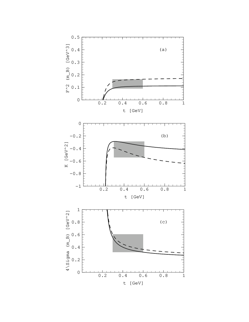
FIG. 5.: The sum rules (53) to leading–order accuracy (i.e. using the spectral densities (51)) as functions of the Borel parameter $t$ for different values of the continuum threshold $\omega_{0}$ (solid lines: $\omega_{0}=1.0\,\text{GeV}$ [$\bar{\Lambda}=0.4\,\text{GeV}$], dashed lines: $\omega_{0}=1.2\,\text{GeV}$ [$\bar{\Lambda}=0.5\,\text{GeV}$]). The shaded areas indicate the working regions of the sum rules. (a) $F^{2}(\mu=m_{B})$, (b) the kinetic energy $K$, (c) $m_{V}^{2}-m_{P}^{2}=4\Sigma$ at the scale $\mu=m_{B}$.

  

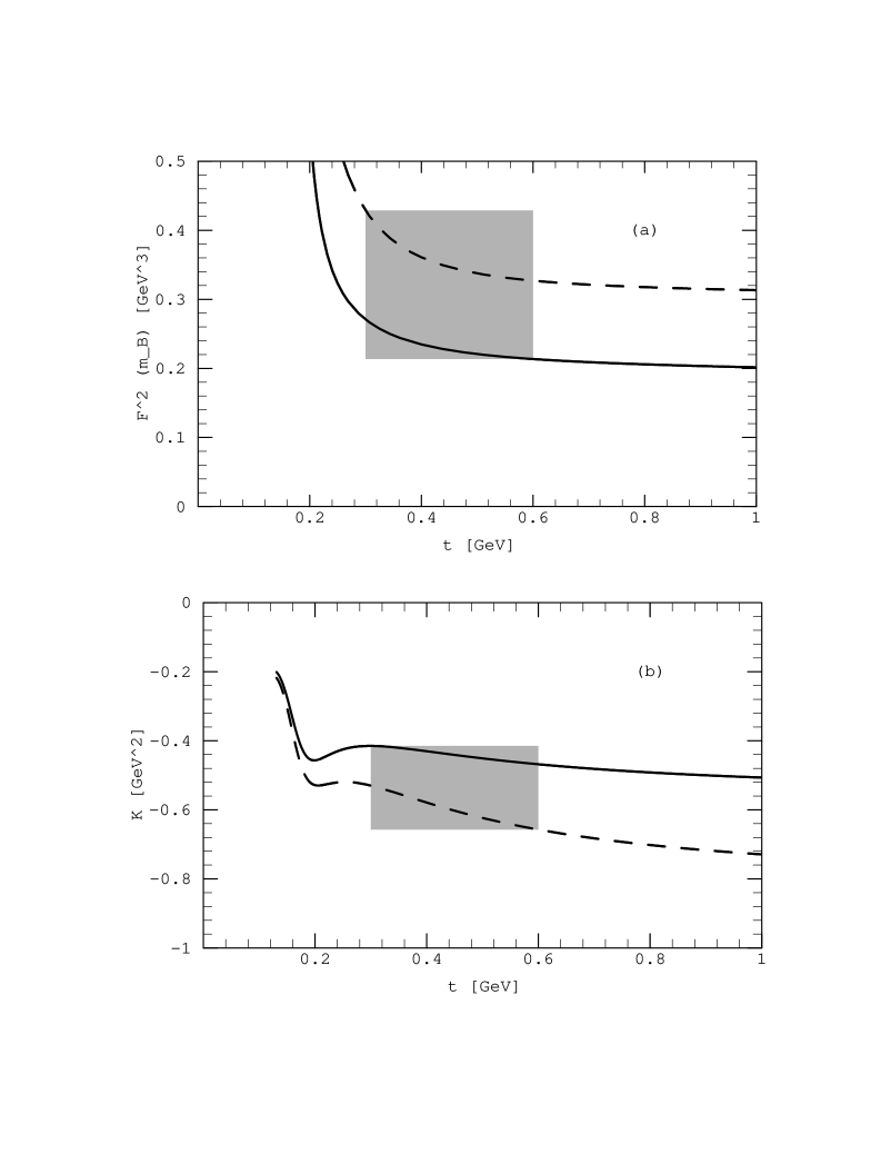
FIG. 6.: The sum rules (70) and (81) in next–to–leading order accuracy. The parameter values are the same as in Fig. 5. (a) $F^{2}(\mu=m_{B})$, (b) the kinetic energy $K$.

REFERENCES

- [1] M.B. Wise, in Proceedings of th 6th Lake Louise Winter Institute, Lake Louise, 1991, edited by B. Campbell et al. (World Scientific, Singapore, 1991), p. 222; H. Georgi, in Proceedings of the TASI 1991, Boulder, 1991, edited by R.K. Ellis, C.T. Hill, and J.O. Sykken (World Scientific, Singapore, 1992), p. 589.
- [2] C.W. Bernard, J.N. Labrenz, and A. Soni, Report hep-lat/9306009.
- [3] E. Bagan et al., Phys. Lett. B 278, 457 (1992).
- [4] M. Neubert, Phys. Rev. D 46, 1076 (1992).
- [5] P. Ball, Phys. Lett. B 281, 133 (1992).
- [6] A.F. Falk, B. Grinstein, and M.E. Luke, Nucl. Phys. B357, 185 (1991).
- [7] T. Mannel, W. Roberts, Z. Ryzak, Nucl. Phys. B 368, 204 (1992)
- [8] A.F. Falk, M. Neubert, Phys. Rev. D 47, 2965, 2982 (1993).
- [9] I.I. Bigi, N.G. Uraltsev, and A.I. Vainstein, Phys. Lett. B 293, 430 (1992).
- [10] L. Maiani, G. Martinelli, and C.T. Sachrajda, Nucl. Phys. B368, 281 (1992).
- [11] M.A. Shifman, A.I. Vainshtein, and V.I. Zakharov, Nucl. Phys. B147, 385, 448, 519 (1979).
- [12] H. Georgi, Phys. Lett. B 240, 447 (1990).
- [13] M. Luke and A.V. Manohar, Phys. Lett. B 286, 348 (1992).
- [14] X. Ji and M.J. Musolf, Phys. Lett. B 257, 409 (1991).
- [15] J.D. Bjorken, in Proceedings of Les Rencontres de Physique de la Vallée d’Aoste, La Thuile, 1990, edited by M. Greco (Editions Frontieres, Gif-sur-Yvette, 1990), p. 583; A. Falk et al., Nucl. Phys. B343, 1 (1990).
- [16] M.A. Shifman and M.B. Voloshin, Sov. J. Nucl. Phys. 45, 292 (1987); 47, 511 (1988).
- [17] D.J. Broadhurst and A.G. Grozin, Phys. Lett. B 267, 105 (1991).
- [18] Vacuum Structure and QCD Sum Rules, Current Physics Sources and Comments, Vol. 10, edited by M.A. Shifman (North–Holland, Amsterdam, 1992).
- [19] N. Isgur and M.B. Wise, Phys. Lett. B 232, 113 (1989); 237, 527 (1990).
- [20] B. Blok, M.A. Shifman, Phys. Rev. D 47, 2949 (1993).
- [21] I.I. Balitskii, A.V. Kolesnichenko, and A.V. Yung, Phys. Lett. B 157, 309 (1985).
- [22] V.M. Braun and A.V. Kolesnichenko, Nucl. Phys. B283, 723 (1987).
- [23] M. Aguilar-Benitez et al., Review of Particle Properties, Phys. Rev. D 45, Part 2 (1992).
- [24] D.J. Broadhurst and A.G. Grozin, Phys. Lett. B 274, 421 (1992).
- [25] P. Ball, V.M. Braun, and H.G. Dosch, Phys. Rev. D 44, 3567 (1991); P. Ball, München Report TUM–T31–39/93 (1993) (to appear in Phys. Rev. D).
- [26] E. Bagan, P. Ball, and P. Gosdzinsky, Phys. Lett. B 301, 249 (1993).
- [27] V. Eletskii, E. Shuryak, Phys. Lett. B 276, 191 (1992).
- [28] M. Neubert, Phys. Rev. D 45, 2451 (1992).
- [29] B. Blok et al., Report hep-ph/9307247.
- [30] V.A. Nesterenko and A.V. Radyushkin, Phys. Lett. B 115, 410 (1982); Sov. Phys. JETP Lett. 35, 488 (1982).
- [31] K.G. Chetyrkin and F.V. Tkachov, Nucl. Phys. B192, 159 (1981).