Two–Loop Anomalous Dimension Matrix for
$\Delta S=1$ Weak Non-Leptonic Decays II: ${\cal O}(\alpha\,\alpha_{\rm s})$

Abstract

We calculate the $10\times 10$ two–loop anomalous dimension matrix to order ${\cal O}(\alpha\,\alpha_{\rm s})$ in the dimensional regularization scheme with anticommuting $\gamma_{5}$ (NDR) which is necessary for the extension of the $\Delta S=1$ weak Hamiltonian involving electroweak penguins beyond the leading logarithmic approximation. We demonstrate, how a direct calculation of penguin diagrams involving $\gamma_{5}$ in closed fermion loops can be avoided thus allowing a consistent calculation of two–loop anomalous dimensions in the simplest renormalization scheme with anticommuting $\gamma_{5}$ in $D$ dimensions. We give the necessary one–loop finite terms which allow to obtain the corresponding two–loop anomalous dimension matrix in the HV scheme with non–anticommuting $\gamma_{5}$.

1 Introduction

The inclusion of next–to–leading QCD corrections to the effective low energy Hamiltonian for non–leptonic decays requires the calculation of the relevant two–loop anomalous dimension matrices. In the case of the $\Delta S=1$ Hamiltonian there are ten operators $Q_{i},i=1,\ldots,10$ to be considered: current–current operators $(i=1,2)$, QCD penguin operators $(i=3,\ldots,6)$ and electroweak penguin operators $(i=7,\ldots,10)$. Consequently, one deals with $10\times 10$ anomalous dimension matrices.

Because of the presence of electroweak penguin operators with Wilson coefficients of ${\cal O}(\alpha)$, a consistent analysis must involve anomalous dimensions resulting from both strong and electromagnetic interactions. Working to first order in $\alpha$ but to all orders in $\alpha_{\rm s}$, the following anomalous dimension matrix is needed for the leading and next–to–leading logarithmic approximation for the Wilson coefficient functions,

$$\hat{\gamma}\;=\;\frac{\alpha_{\rm s}}{4\pi}\,\hat{\gamma}_{\rm s}^{(0)}+\frac{\alpha}{4\pi}\,\hat{\gamma}_{\rm e}^{(0)}+\frac{\alpha_{\rm s}^{2}}{(4\pi)^{2}}\,\hat{\gamma}_{\rm s}^{(1)}+\frac{\alpha\,\alpha_{\rm s}}{(4\pi)^{2}}\,\hat{\gamma}_{\rm se}^{(1)}\,.$$ (1.1)

The one–loop matrices $\hat{\gamma}_{\rm s}^{(0)}$ and $\hat{\gamma}_{\rm e}^{(0)}$ have been calculated long time ago [1]–[11]. The $2\times 2$ submatrix of the two–loop QCD matrix $\hat{\gamma}_{\rm s}^{(1)}$ involving current–current operators $Q_{1}$ and $Q_{2}$ has been calculated in ref. [12, 13]. Recently, we have generalized these two–loop calculations to the penguin operators $Q_{i},i=3,\ldots,10$ [14, 15], so that the full matrix $\hat{\gamma}_{\rm s}^{(1)}$ is also known. The purpose of the present paper is the calculation of $\hat{\gamma}_{\rm se}^{(1)}$.

The calculation of $\hat{\gamma}_{\rm se}^{(1)}$ proceeds in analogy to $\hat{\gamma}_{\rm s}^{(1)}$. In fact all the singularities calculated in ref. [15] can be used here so that our main task was the calculation of the relevant colour and electric charge factors in two–loop diagrams involving one gluon and one photon. Yet as will be seen the structure of basic expressions and of the results differs from the one found in the pure QCD case, because now the electric charges of quarks matter and the flavour symmetries present in ref. [15] are broken. In fact this breakdown of flavour symmetry is the origin of the existence of electroweak penguin operators.

In order to make the comparison with the calculation of $\hat{\gamma}_{\rm s}^{(1)}$ as easy as possible, we have organized the present paper in a similar way as it was done in ref. [15]. We present here however only the results in the naive dimensional regularization with anticommuting $\gamma_{5}$ (NDR). The consistency of the NDR and ’t Hooft–Veltman (HV) scheme for the calculation at hand has been demonstrated in ref. [15]. There we have developed a method which allows to avoid a direct calculation of penguin diagrams involving $\gamma_{5}$ in closed fermion loops which are ambiguous in the case of the NDR scheme. Our method can be generalized to the present case so that an unambiguous calculation of $\hat{\gamma}_{\rm se}^{(1)}$ can be accomplished in the NDR scheme. This is gratifying because this scheme is certainly the most convenient and contrary to the HV scheme [16, 13, 17] satisfies all Ward–identities in the context of the minimal subtraction scheme.

Our paper is organized as follows: In section 2, we recall the explicit expressions for the operators $Q_{i}$, and we classify the one– and two–loop diagrams into current–current and penguin diagrams. We also discuss the basic formalism necessary for the calculation of $\hat{\gamma}_{\rm se}^{(1)}$. In section 3, we recall the matrix $\hat{\gamma}_{\rm e}^{(0)}$. In section 4, the calculations and results for two–loop current–current diagrams are presented. In section 5, an analogous presentation is given for two–loop penguin diagrams. In section 6, we combine the results of the previous sections to obtain $\hat{\gamma}_{\rm se}^{(1)}$ in the NDR scheme. We discuss various properties of this matrix, in particular its Large–N limit. Section 7 contains a brief summary of our paper. In appendices A and B, explicit expressions for the elements of the $10\times 10$ matrices $\hat{\gamma}_{\rm e}^{(0)}$ and $\hat{\gamma}_{\rm se}^{(1)}$ for arbitrary numbers of colours ($N$) and flavours ($f$) are given. In appendix C, the corresponding results for $\hat{\gamma}_{\rm se}^{(1)}$ in the case of $N=3$ are presented.

2 General Formalism

2.1 Operators

The ten operators considered in this paper are given as follows

$$Q_{1} = \left(\bar{s}_{\alpha}u_{\beta}\right)_{\rm V-A}\left(\bar{u}_{\beta}d_{\alpha}\right)_{\rm V-A}\,,$$

$$Q_{2} = \left(\bar{s}u\right)_{\rm V-A}\left(\bar{u}d\right)_{\rm V-A}\,,$$

$$Q_{3} = \left(\bar{s}d\right)_{\rm V-A}\sum_{q}\left(\bar{q}q\right)_{\rm V-A}\,,$$

$$Q_{4} = \left(\bar{s}_{\alpha}d_{\beta}\right)_{\rm V-A}\sum_{q}\left(\bar{q}_{\beta}q_{\alpha}\right)_{\rm V-A}\,,$$

$$Q_{5} = \left(\bar{s}d\right)_{\rm V-A}\sum_{q}\left(\bar{q}q\right)_{\rm V+A}\,,$$

$$Q_{6} = \left(\bar{s}_{\alpha}d_{\beta}\right)_{\rm V-A}\sum_{q}\left(\bar{q}_{\beta}q_{\alpha}\right)_{\rm V+A}\,,$$ (2.1)

$$Q_{7} = \frac{3}{2}\left(\bar{s}d\right)_{\rm V-A}\sum_{q}e_{q}\left(\bar{q}q\right)_{\rm V+A}\,,$$

$$Q_{8} = \frac{3}{2}\left(\bar{s}_{\alpha}d_{\beta}\right)_{\rm V-A}\sum_{q}e_{q}\left(\bar{q}_{\beta}q_{\alpha}\right)_{\rm V+A}\,,$$

$$Q_{9} = \frac{3}{2}\left(\bar{s}d\right)_{\rm V-A}\sum_{q}e_{q}\left(\bar{q}q\right)_{\rm V-A}\,,$$

$$Q_{10} = \frac{3}{2}\left(\bar{s}_{\alpha}d_{\beta}\right)_{\rm V-A}\sum_{q}e_{q}\left(\bar{q}_{\beta}q_{\alpha}\right)_{\rm V-A}\,,$$

where $\alpha$, $\beta$ denote colour indices ($\alpha,\beta=1,\ldots,N$) and $e_{q}$ are quark charges. We omit the colour indices for the colour singlet operators. $(V\pm A)$ refer to $\gamma_{\mu}(1\pm\gamma_{5})$. This basis closes under QCD and QED renormalization.

At one stage it will be useful to study other bases, in particular the basis in which the first two operators are replaced by their Fierz conjugates,

$$\widetilde{Q}_{1} = \left(\bar{s}d\right)_{\rm V-A}\left(\bar{u}u\right)_{\rm V-A}\,,$$

$$\widetilde{Q}_{2} = \left(\bar{s}_{\alpha}d_{\beta}\right)_{\rm V-A}\left(\bar{u}_{\beta}u_{\alpha}\right)_{\rm V-A}\,,$$ (2.2)

with remaining operators unchanged. In fact the latter basis is the one used by Gilman and Wise [4]. We prefer however to put $Q_{2}$ in the colour singlet form as in eq. (2.1), because it is this form in which this operator enters the tree level Hamiltonian. Let us finally recall that the Fierz conjugates of the $(V-A)\otimes(V+A)$ operators $Q_{i},\;i=5,\ldots,8$ are given by

$$\widetilde{Q}_{6} = -\,8\sum_{q}\left(\bar{s}_{\rm L}q_{\rm R}\right)\left(\bar{q}_{\rm R}d_{\rm L}\right)\,,$$

$$\widetilde{Q}_{8} = -\,12\sum_{q}e_{q}\left(\bar{s}_{\rm L}q_{\rm R}\right)\left(\bar{q}_{\rm R}d_{\rm L}\right)\,,$$ (2.3)

with similar expressions for $\widetilde{Q}_{5}$ and $\widetilde{Q}_{7}$. Here $q_{R,L}=\frac{1}{2}(1\pm\gamma_{5})q$. The Fierz conjugates of the $(V-A)\otimes(V-A)$ penguin operators $Q_{3},Q_{4},Q_{9}$, and $Q_{10}$ to be denoted by $\widetilde{Q}_{i},\;i=3,4,9,10$ are found in analogy to (2.2).

2.2 Classification of Diagrams

In order to calculate the anomalous dimension matrices $\hat{\gamma}_{\rm e}^{(0)}$ and $\hat{\gamma}_{\rm se}^{(1)}$, one has to insert the operators of eq. (2.1) in appropriate four–point functions and extract $1/\varepsilon$ divergences. The precise relation between $1/\varepsilon$ divergences in one– and two–loop diagrams and one– and two–loop anomalous dimension matrices will be given in the following subsection. Here, let us only recall that insertion of any of the operators of eq. (2.1) into the diagrams discussed below results into a linear combination of the operators $Q_{i}$. The row in the anomalous dimension matrix corresponding to the inserted operator can then be obtained from the coefficients in the linear combination in question.

There are three basic ways a given operator can be inserted in a four–point function. They are shown in fig. 1, where the dot denotes the interaction described by a current in a given operator of eq. (2.1) and the wavy line denotes a gluon or a photon.

We will refer to the insertions of fig. 1(a) as “current–current” insertions. The insertions of fig. 1(b) and (c) will then be called “penguin insertions” of type 1 and type 2 respectively.

The complete list of diagrams necessary for one– and two–loop calculations is given in figs. 2–5. At one–loop level one has three current–current diagrams (fig. 2) to be denoted as in ref. [13] by $D_{1}$ – $D_{3}$, and one penguin diagram (fig. 3) of each type to be denoted by $P_{0}^{(1)}$ and $P_{0}^{(2)}$ for type 1 and type 2 insertions respectively. At two–loop level there are 21 current–current diagrams shown in fig. 4, to be denoted by $D_{4}$ – $D_{24}$ , and 12 penguin diagrams of each type shown in fig. 5 to be denoted by $P_{1}^{(1)}$ –$P_{14}^{(1)}$ and $P_{1}^{(2)}$ –$P_{14}^{(2)}$ respectively. The notation is similar to ref.[15], but this time the wavy lines denote a gluon or photon so that complete ${\cal O}(\alpha\,\alpha_{\rm s})$ is obtained. The omitted diagrams $P_{6}$ and $P_{7}$ having triple boson vertices do not contribute here. The penguin diagrams which have no $1/\varepsilon$ divergences and some examples of penguin diagrams which vanish identically in dimensional regularization are given in figs. 6 and 7 of ref. [15]. It is needless to say that all possible permutations of gluons and photons have to be considered as well as left–right reflections. In the case of current–currrent diagrams also up–down reflections have to be considered.

2.3 Basic Formulae for Anomalous Dimensions

The anomalous dimensions of the operators $Q_{i}$, calculated in the $\overline{\rm MS}$ scheme, are obtained from the $1/\varepsilon$ divergences of the relevant one– and two–loop diagrams with $Q_{i}$ insertions and from the $1/\varepsilon$ divergences in the quark wave–function renormalization. Let us denote by $\vec{Q}$ a column vector composed of operators $Q_{i}$. Then

$$\hat{\gamma}(g,e)=\hat{Z}^{-1}\mu\frac{\partial}{\partial\mu}\hat{Z},\qquad\vec{Q}_{\rm B}=\hat{Z}\;\vec{Q}\,,$$ (2.4)

where $\vec{Q}_{\rm B}$ stands for bare operators. Working in $D=4-2\,\varepsilon$ dimensions, we can expand $\hat{Z}$ in inverse powers of $\varepsilon$ as follows

$$\hat{Z}=\hat{1}+\sum_{k=1}^{\infty}\frac{1}{\varepsilon^{k}}\hat{Z}_{k}(g,e)\,,$$ (2.5)

where $g$ and $e$ are the QCD and QED renormalized coupling constants.

Inserting (2.5) into (2.4), one derives a useful result

$$\hat{\gamma}(g,e)\;=\;-\,2g^{2}\frac{\partial\hat{Z}_{1}(g,e)}{\partial g^{2}}-2e^{2}\frac{\partial\hat{Z}_{1}(g,e)}{\partial e^{2}}\,.$$ (2.6)

Let us next denote by $\Gamma^{(4)}(\vec{Q})$ and $\Gamma_{B}^{(4)}(\vec{Q}^{B})$ the renormalized and the bare four–quark Green functions with operator $\vec{Q}$ insertions. Strictly speaking $\Gamma^{(4)}(\vec{Q})$ and $\Gamma_{B}^{(4)}(\vec{Q}^{B})$ are matrices, because the insertion of a single operator in a given diagram results in a linear combination of operators.

At the one–loop level $\Gamma_{B}^{(4)}$ is obtained by evaluating the diagrams of figs. 2 and 3. At the two–loop level it is found by evaluating the diagrams of figs. 4 and 5 and subtracting the corresponding two–loop counter terms. Next

$$\Gamma^{(4)}(\vec{Q})=\hat{Z}_{\psi}\hat{Z}^{-1}\Gamma_{\rm B}^{(4)}(\vec{Q}_{\rm B})\,,$$ (2.7)

where $\hat{Z}_{\psi}$ is a matrix which represents the renormalization of the four quark fields on external lines. In the pure QCD case this matrix was diagonal. The ${\cal O}(\alpha)$ and ${\cal O}(\alpha\,\alpha_{\rm s})$ terms in this matrix are however non–diagonal, because in the case of penguin operators the $d\bar{d}$, $s\bar{s}$, and $b\bar{b}$ parts are renormalized differently from $u\bar{u}$ and $c\bar{c}$ parts. We next expand $\Gamma_{\rm B}^{(4)}$ and $\hat{Z}_{\psi}$ in inverse powers of $\varepsilon$ as follows

$$\hat{Z}_{\psi}=\hat{1}+\sum_{k=1}^{\infty}\frac{1}{\varepsilon^{k}}\hat{Z}_{\psi,k}(g,e)\,,$$ (2.8)

$$\Gamma_{\rm B}^{(4)}(Q_{i})=1+\sum_{k=1}^{\infty}\frac{1}{\varepsilon^{k}}Z^{(\Gamma)}_{k}(g,e,Q_{i})+{\rm finite}\,,$$ (2.9)

where

$$\hat{Z}_{\psi,1}(g,e)=\frac{e^{2}}{(4\pi)^{2}}\hat{Z}_{\psi}^{(0)}+\frac{e^{2}\,g^{2}}{(4\pi)^{4}}\hat{Z}_{\psi}^{(1)}+\ldots\,,$$ (2.10)

$$Z^{(\Gamma)}_{1}(g,e,Q_{i})=\sum_{j=1}^{10}\left(\frac{e^{2}}{(4\pi)^{2}}(d_{1})_{ij}+\frac{e^{2}\,g^{2}}{(4\pi)^{4}}(d_{2})_{ij}+\ldots\right)\,,$$ (2.11)

where the dots stand for the pure QCD case which has been already considered in ref. [15] and higher order corrections.

Demanding $\Gamma^{(4)}$ to be finite, we find $\hat{Z}_{1}(g,e)$ and using (2.6)

$$\left(\hat{\gamma}_{\rm e}^{(0)}\right)_{ij} = -\,2\left[(\hat{Z}_{\psi}^{(0)})_{ij}+(d_{1})_{ij}\right]\,,$$ (2.12)

$$\left(\hat{\gamma}_{\rm se}^{(1)}\right)_{ij} = -\,4\left[(\hat{Z}_{\psi}^{(1)})_{ij}+(d_{2})_{ij}\right]\,.$$ (2.13)

The matrices $\hat{Z}_{\psi}^{(0)}$ and $\hat{Z}_{\psi}^{(1)}$ are given in section 2.5.

2.4 Renormalization Scheme Dependence of $\hat{\gamma}_{\rm se}^{(1)}$

The two–loop anomalous dimension matrix $\hat{\gamma}_{\rm se}^{(1)}$ depends on the renormalization scheme for operators and in particular on the treatment of $\gamma_{5}$ in $D\not=4$ dimensions. This is signaled by the scheme dependence of the finite terms $\hat{r}_{\rm s}$ and $\hat{r}_{\rm e}$ in the renormalized one–loop matrix elements

$$\langle\vec{Q}\rangle=\left[\hat{1}+\frac{\alpha_{\rm s}}{4\pi}\hat{r}_{\rm s}+\frac{\alpha}{4\pi}\hat{r}_{\rm e}\right]\langle\vec{Q}^{(0)}\rangle\,,$$ (2.14)

where $\langle\vec{Q}^{(0)}\rangle$ denotes tree–level matrix elements.

If $\hat{Z}_{a}$ and $\hat{Z}_{b}$ are two renormalization factors of (2.4) corresponding to two renormalization schemes $a$ and $b$, then

$$\hat{Z}_{a}=\hat{Z}_{b}\left[\hat{1}+\frac{\alpha_{\rm s}}{4\pi}\Delta\hat{r}_{\rm s}+\frac{\alpha}{4\pi}\Delta\hat{r}_{\rm e}\right]\,,$$ (2.15)

where

$$\Delta\hat{r}_{\rm s}=(\hat{r}_{\rm s})_{b}-(\hat{r}_{\rm s})_{a}\,,\qquad\Delta\hat{r}_{\rm e}=(\hat{r}_{\rm e})_{b}-(\hat{r}_{\rm e})_{a}\,.$$ (2.16)

Using eqs. (2.15) and (2.4) one finds the relation between $\hat{\gamma}_{\rm se}^{(1)}$ calculated in schemes $a$ and $b$.

$$\left(\hat{\gamma}_{\rm se}^{(1)}\right)_{b}\;=\;\left(\hat{\gamma}_{\rm se}^{(1)}\right)_{a}+\left[\Delta\hat{r}_{\rm s},\hat{\gamma}_{\rm e}^{(0)}\right]+\left[\Delta\hat{r}_{\rm e},\hat{\gamma}_{\rm s}^{(0)}\right]\,.$$ (2.17)

This relation is very useful as it allows to test the compatibility of the two–loop anomalous dimensions calculated in different renormalization schemes and plays a role in the proof of scheme independence of physical quantities as demonstrated in ref. [18].

2.5 The Matrices $\hat{Z}_{\psi}^{(0)}$ and $\hat{Z}_{\psi}^{(1)}$

We give here the matrices $\hat{Z}_{\psi}^{(0)}$ and $\hat{Z}_{\psi}^{(1)}$ in the Feynman gauge. The wave–function renormalization for a quark of charge $q$ is given in the Feynman gauge by

$$Z^{(\psi)}=1-\frac{\alpha}{4\pi}\frac{1}{\varepsilon}\,q^{2}+\frac{\alpha\,\alpha_{\rm s}}{(4\pi)^{2}}\frac{1}{\varepsilon}\,\frac{3}{2}\,q^{2}C_{F}+\ldots\,,$$ (2.18)

where the dots denote terms which are of no interest to us here, and

$$C_{F}=\frac{N^{2}-1}{2N}\,.$$ (2.19)

Applying the renormalization (2.18) to the quark fields in the operators $Q_{i}$ according to

$$\psi_{\rm B}=Z_{\psi}^{1/2}\psi\,,$$ (2.20)

one finds the matrices $\hat{Z}_{\psi}^{(0)}$ and $\hat{Z}_{\psi}^{(1)}$. They are given by a single matrix $\hat{D}$

$$\hat{Z}_{\psi}^{(0)}=-\hat{D},\qquad\hat{Z}_{\psi}^{(1)}=\frac{3}{2}\,C_{F}\hat{D}\,.$$ (2.21)

The non–vanishing elements of $\hat{D}$ are

$$\begin{array}[]{ccccccccc}\hat{D}(1,1)&=&\hat{D}(2,2)&=&\frac{5}{9}\,,&&&&\\ \hat{D}(3,3)&=&\hat{D}(4,4)&=&\hat{D}(5,5)&=&\hat{D}(6,6)&=&\frac{1}{3}\,,\\ \hat{D}(3,9)&=&\hat{D}(4,10)&=&\hat{D}(5,7)&=&\hat{D}(6,8)&=&\frac{2}{9}\,,\\ \hat{D}(7,7)&=&\hat{D}(8,8)&=&\hat{D}(9,9)&=&\hat{D}(10,10)&=&\frac{4}{9}\,,\\ \hat{D}(7,5)&=&\hat{D}(8,6)&=&\hat{D}(9,3)&=&\hat{D}(10,4)&=&\frac{1}{9}\,.\end{array}$$ (2.22)

3 One-Loop Results

We give here one–loop results in QED. The corresponding QCD expressions can be found in section 3 of ref. [15].

3.1 Current-Current Contributions to $\hat{\gamma}_{\rm e}^{(0)}$

The non–vanishing contributions of diagrams $D_{1}$ – $D_{3}$ of fig. 2 to the matrix $\hat{\gamma}_{\rm e}^{(0)}$ are given as follows

$$\begin{array}[]{ccccccccc}\left[\hat{\gamma}_{\rm e}^{(0)}(1,1)\right]_{\rm cc}&=&\left[\hat{\gamma}_{\rm e}^{(0)}(2,2)\right]_{\rm cc}&=&\left[\hat{\gamma}_{\rm e}^{(0)}(3,9)\right]_{\rm cc}&=&\left[\hat{\gamma}_{\rm e}^{(0)}(4,10)\right]_{\rm cc}&=&-\frac{8}{3}\,,\\ \vbox{\vskip 14.22636pt}\left[\hat{\gamma}_{\rm e}^{(0)}(5,7)\right]_{\rm cc}&=&\left[\hat{\gamma}_{\rm e}^{(0)}(6,8)\right]_{\rm cc}&=&\frac{8}{3}\,,&&&&\\ \vbox{\vskip 14.22636pt}\left[\hat{\gamma}_{\rm e}^{(0)}(7,5)\right]_{\rm cc}&=&\left[\hat{\gamma}_{\rm e}^{(0)}(7,7)\right]_{\rm cc}&=&\left[\hat{\gamma}_{\rm e}^{(0)}(8,6)\right]_{\rm cc}&=&\left[\hat{\gamma}_{\rm e}^{(0)}(8,8)\right]_{\rm cc}&=&\frac{4}{3}\,,\\ \vbox{\vskip 14.22636pt}\left[\hat{\gamma}_{\rm e}^{(0)}(9,3)\right]_{\rm cc}&=&\left[\hat{\gamma}_{\rm e}^{(0)}(9,9)\right]_{\rm cc}&=&\left[\hat{\gamma}_{\rm e}^{(0)}(10,4)\right]_{\rm cc}&=&\left[\hat{\gamma}_{\rm e}^{(0)}(10,10)\right]_{\rm cc}&=&-\frac{4}{3}\,.\end{array}$$ (3.1)

These results already include the contributions from the wave function renormalization.

3.2 Penguin Contributions to $\hat{\gamma}_{\rm e}^{(0)}$

The contributions of diagrams $P_{0}^{(1)}$ and $P_{0}^{(2)}$ of fig. 3 to the matrix $\hat{\gamma}_{\rm e}^{(0)}$ have a very simple structure. The insertion of any operator of (2.1) into the diagrams of fig. 3 results always into the sum of the operators $Q_{7}$ and $Q_{9}$ multiplied by an overall factor. Denoting by

$$\bar{P}\;=\;\left(0,0,0,0,0,0,1,0,1,0\right)$$ (3.2)

the row vector in the space $(Q_{1},\ldots,Q_{10})$, the elements of $\hat{\gamma}_{\rm e}^{(0)}$ coming from the diagrams of fig. 3 are as follows

$$\begin{array}[]{rclrcl}\left[\hat{\gamma}_{\rm e}^{(0)}(Q_{1})\right]_{\rm p}&=&\frac{16}{27}N\bar{P}\,,&\left[\hat{\gamma}_{\rm e}^{(0)}(Q_{2})\right]_{\rm p}&=&\frac{16}{27}\bar{P}\,,\\ \left[\hat{\gamma}_{\rm e}^{(0)}(Q_{3})\right]_{\rm p}&=&\frac{16}{27}N\left(u-\frac{d}{2}-\frac{1}{N}\right)\bar{P}\,,&\left[\hat{\gamma}_{\rm e}^{(0)}(Q_{4})\right]_{\rm p}&=&\frac{16}{27}\left(u-\frac{d}{2}-N\right)\bar{P}\,,\\ \left[\hat{\gamma}_{\rm e}^{(0)}(Q_{5})\right]_{\rm p}&=&\frac{16}{27}N\left(u-\frac{d}{2}\right)\bar{P}\,,&\left[\hat{\gamma}_{\rm e}^{(0)}(Q_{6})\right]_{\rm p}&=&\frac{16}{27}\left(u-\frac{d}{2}\right)\bar{P}\,,\\ \left[\hat{\gamma}_{\rm e}^{(0)}(Q_{7})\right]_{\rm p}&=&\frac{16}{27}N\left(u+\frac{d}{4}\right)\bar{P}\,,&\left[\hat{\gamma}_{\rm e}^{(0)}(Q_{8})\right]_{\rm p}&=&\frac{16}{27}\left(u+\frac{d}{4}\right)\bar{P}\,,\\ \left[\hat{\gamma}_{\rm e}^{(0)}(Q_{9})\right]_{\rm p}&=&\frac{16}{27}N\left(u+\frac{d}{4}+\frac{1}{2N}\right)\bar{P}\,,&\left[\hat{\gamma}_{\rm e}^{(0)}(Q_{10})\right]_{\rm p}&=&\frac{16}{27}\left(u+\frac{d}{4}+\frac{N}{2}\right)\bar{P}\,,\end{array}$$ (3.3)

where $u$ and $d$ ($u+d=f$) denote the number of effective up– and down–quark flavours, respectively.

It should be stressed that these results do not depend on renormalization scheme for $Q_{i}$ and are also valid for $\widetilde{Q}_{i}$.

3.3 General Comments on $\hat{r}$

As already remarked in section 2.4, the finite terms $\hat{r}_{\rm s}$ and $\hat{r}_{\rm e}$ depend on the renormalization scheme used. In the case of the NDR scheme considered here, the penguin diagram contributions to these finite terms may also depend on whether $Q_{i}$ or their Fierz conjugates $\widetilde{Q}_{i}$ are inserted in the penguin diagrams. This observation has already been made in ref. [15] and has been used to avoid a direct evaluation of the two–loop diagrams involving $Tr(\gamma_{5}\gamma_{\mu}\gamma_{\nu}\gamma_{\tau}\gamma_{\sigma})$, i.e. the type 1 penguin insertions. Here we only state that whereas the results for $(V-A)\otimes(V+A)$ operators $Q_{5}$–$Q_{8}$ do not depend on the form used, this is no longer the case for the $(V-A)\otimes(V-A)$ operators $Q_{1}$–$Q_{4}$, $Q_{9}$, and $Q_{10}$. We will return to this in section 5.1, where a generalization of the method of ref. [15] to the mixed QED–QCD case is presented.

4 Current-Current Contributions to the ${\cal O}(\alpha\,\alpha_{\rm s})$ Anomalous Dimension Matrix $\hat{\gamma}_{\rm se}^{(1)}$

The calculation of current–current contributions to the ${\cal O}(\alpha\,\alpha_{\rm s})$ anomalous dimension matrix $\hat{\gamma}_{\rm se}^{(1)}$ uses the singularities found in our previous calculation of the ${\cal O}(\alpha_{\rm s}^{2})$ contributions. Due to the fact that certain diagrams present in the pure QCD case do not contribute here and due to different colour and electric charge factors, the basic structure of the ${\cal O}(\alpha\,\alpha_{\rm s})$ results is quite different from pure QCD. In particular, the mixing between different operators can be divided into three blocks $(Q_{1},Q_{2})$, $(Q_{3},Q_{4},Q_{9},Q_{10})$ and $(Q_{5},Q_{6},Q_{7},Q_{8})$ with no mixing between different blocks.

The results in this section include the contribution of the matrix $\hat{Z}_{\psi}^{(1)}$.

4.1 $(V-A)\otimes(V-A)$ Operators

The $2\times 2$ matrix describing the mixing in the current–current sector $(Q_{1},Q_{2})$ is given by

$$\left(\begin{array}[]{cc}8N-\frac{22}{3}\frac{1}{N}&-\,\frac{2}{3}\vbox{\vskip 14.22636pt}\\ \frac{25}{3}&-N-\frac{22}{3}\frac{1}{N}\end{array}\right)\,.$$ (4.1)

The $4\times 4$ matrix describing the mixing in the current–current sector $(Q_{3},Q_{4},Q_{9},Q_{10})$ is given by

$$\left(\begin{array}[]{cccc}\frac{6}{N}&-\,6&8N-\frac{40}{3}\frac{1}{N}&\frac{16}{3}\vbox{\vskip 14.22636pt}\\ -\,3&-\,3N+\frac{6}{N}&\frac{34}{3}&2N-\frac{40}{3}\frac{1}{N}\vbox{\vskip 14.22636pt}\\ 4N-\frac{20}{3}\frac{1}{N}&\frac{8}{3}&4N-\frac{2}{3}\frac{1}{N}&-\,\frac{10}{3}\\ \vbox{\vskip 14.22636pt}\frac{17}{3}&N-\frac{20}{3}\frac{1}{N}&\frac{8}{3}&-\,2N-\frac{2}{3}\frac{1}{N}\vbox{\vskip 14.22636pt}\end{array}\right)\,.$$ (4.2)

4.2 $(V-A)\otimes(V+A)$ Operators

The $4\times 4$ matrix describing the mixing in the current–current sector $(Q_{5},Q_{6},Q_{7},Q_{8})$ is given by

$$\left(\begin{array}[]{cccc}-\,\frac{6}{N}&6&-\,8N-\frac{16}{3}\frac{1}{N}&\frac{40}{3}\\ \vbox{\vskip 14.22636pt}3&3N-\frac{6}{N}&-\,2&\frac{22}{3}N-\frac{16}{3}\frac{1}{N}\\ \vbox{\vskip 14.22636pt}-\,4N-\frac{8}{3}\frac{1}{N}&\frac{20}{3}&-\,4N-\frac{26}{3}\frac{1}{N}&\frac{38}{3}\\ \vbox{\vskip 14.22636pt}-\,1&\frac{11}{3}N-\frac{8}{3}\frac{1}{N}&2&\frac{20}{3}N-\frac{26}{3}\frac{1}{N}\end{array}\right)\,.$$ (4.3)

We observe that the elements of both matrices grow at most as $N$ in the Large–$N$ limit and consequently the anomalous dimension matrix ${\cal O}(\alpha\,\alpha_{\rm s})$ resulting from current–current diagrams approaches a constant $N$–independent matrix.

5 Penguin Diagram Contributions to the ${\cal O}(\alpha\,\alpha_{\rm s})$ Anomalous Dimension Matrix $\hat{\gamma}_{\rm se}^{(1)}$

5.1 General Structure

The calculation of the penguin diagram contributions to $\hat{\gamma}_{\rm se}^{(1)}$ can be considerably simplified by first analyzing the general structure of these contributions. The two–loop penguin diagrams are shown in fig. 5 where two types of insertions of a given operator, type 1 and type 2, have to be considered. It is known that type 1 insertions are problematic in the NDR scheme in which closed fermion loops involving $\gamma_{5}$ can not be calculated unambiguously. Yet, as we have demonstrated in our previous paper, the calculation of ${\cal O}(\alpha_{\rm s}^{2})$ anomalous dimensions can be reduced to the calculation of type 2 insertions only. Type 2 insertions do not pose any problems. Indeed with the help of eq. (2.17) with $a$ and $b$ standing this time for two different bases (see eqs. (2.1) and (2.2)) it is possible to relate the type 1 insertions to the type 2 insertions. This procedure can be generalized to ${\cal O}(\alpha\,\alpha_{\rm s})$ so that also in this case explicit calculations of closed fermion loops can be avoided. The procedure this time is more complicated because the insertions of operators involving $\bar{u}u$ have to be distinguished from the insertions of operators involving $\bar{d}d$. We will now explain the procedure in some detail.

In order to solve the problem of closed fermion loops involving $\gamma_{5}$ in the NDR scheme, we have to consider four different bases of operators. All four bases contain the penguin operators $Q_{3}$ – $Q_{10}$ of (2.1) but differ in the current–current operators $Q_{1}$ and $Q_{2}$. The latter are given as follows,

Basis A:

$$Q_{1}^{(u)}\;=\;\left(\bar{s}_{\alpha}u_{\beta}\right)_{V-A}\left(\bar{u}_{\beta}d_{\alpha}\right)_{V-A}\,,\qquad Q_{2}^{(u)}\;=\;\left(\bar{s}u\right)_{V-A}\left(\bar{u}d\right)_{V-A}\,.$$ (5.1)

Basis B:

$$Q_{1}^{(d)}\;=\;\left(\bar{s}_{\alpha}d_{\beta}\right)_{V-A}\left(\bar{d}_{\beta}d_{\alpha}\right)_{V-A}\,,\qquad Q_{2}^{(d)}\;=\;\left(\bar{s}d\right)_{V-A}\left(\bar{d}d\right)_{V-A}\,.$$ (5.2)

Basis C:

$$\widetilde{Q}_{1}^{(u)}\;=\;\left(\bar{s}d\right)_{V-A}\left(\bar{u}u\right)_{V-A}\,,\qquad\widetilde{Q}_{2}^{(u)}\;=\;\left(\bar{s}_{\alpha}d_{\beta}\right)_{V-A}\left(\bar{u}_{\beta}u_{\alpha}\right)_{V-A}\,.$$ (5.3)

Basis D:

$$\widetilde{Q}_{1}^{(d)}\;=\;\left(\bar{s}d\right)_{V-A}\left(\bar{d}d\right)_{V-A}\,,\qquad\widetilde{Q}_{2}^{(d)}\;=\;\left(\bar{s}_{\alpha}d_{\beta}\right)_{V-A}\left(\bar{d}_{\beta}d_{\alpha}\right)_{V-A}\,.$$ (5.4)

The basis A is the standard basis of (2.1) and the basis B is an auxiliary basis needed for the solution of the problem. The bases C and D are simply Fierz conjugates of $Q_{1}$ and $Q_{2}$ in A and B, respectively. Evidently,

$$Q_{1}^{(d)}\;=\;\widetilde{Q}_{2}^{(d)}\,,\qquad Q_{2}^{(d)}\;=\;\widetilde{Q}_{1}^{(d)}\,.$$ (5.5)

Let us next denote by $[Q_{i}]_{1}$ and $[Q_{i}]_{2}$ the result of the type 1 and type 2 insertions of an operator $Q_{i}$, respectively. Then the results for penguin contributions to the row entries of $\hat{\gamma}_{\rm se}^{(1)}$ for $Q_{3}$, $Q_{4}$, $Q_{9}$, and $Q_{10}$ can be written as follows

$${[Q_{3}]_{\rm p}} = u\,[\widetilde{Q}_{1}^{(u)}]_{1}+d\,[\widetilde{Q}_{1}^{(d)}]_{1}+2\,[\widetilde{Q}_{1}^{(d)}]_{2}\,,$$ (5.6)

$$\vbox{\vskip 14.22636pt}{[Q_{4}]_{\rm p}} = u\,[\widetilde{Q}_{2}^{(u)}]_{1}+d\,[\widetilde{Q}_{2}^{(d)}]_{1}+2\,[\widetilde{Q}_{2}^{(d)}]_{2}\,,$$ (5.7)

$$\vbox{\vskip 14.22636pt}{[Q_{9}]_{\rm p}} = u\,[\widetilde{Q}_{1}^{(u)}]_{1}-\frac{d}{2}\,[\widetilde{Q}_{1}^{(d)}]_{1}-[\widetilde{Q}_{1}^{(d)}]_{2}\,,$$ (5.8)

$$\vbox{\vskip 14.22636pt}{[Q_{10}]_{\rm p}} = u\,[\widetilde{Q}_{2}^{(u)}]_{1}-\frac{d}{2}\,[\widetilde{Q}_{2}^{(d)}]_{1}-[\widetilde{Q}_{2}^{(d)}]_{2}\,.$$ (5.9)

Evidently, in order to calculate these rows, the problem of closed fermion loops has to be considered. $[Q_{1}]_{\rm p}$ and $[Q_{2}]_{\rm p}$ receive contributions only from type 2 insertions, i.e.

$$[Q_{1}]_{\rm p}\;=\;[Q_{1}^{(u)}]_{2}\,,\qquad[Q_{2}]_{\rm p}\;=\;[Q_{2}^{(u)}]_{2}\,,$$ (5.10)

and do not pose any problems. The case of $(V-A)\otimes(V+A)$ operators will be discussed below.

There are six independent entries in eqs. (5.6) – (5.9), which have to be found in order to complete the calculation. We show how this can be done in four steps:

Step 1:

$[\widetilde{Q}_{1}^{(d)}]_{2}$ and $[\widetilde{Q}_{2}^{(d)}]_{2}$ can be calculated without any problems. The results are given in section 5.2. Moreover one finds the relation

$$[\widetilde{Q}_{2}^{(d)}]_{2}\;=\;-\,\frac{1}{2}\,[Q_{1}^{(u)}]_{2}\,.$$ (5.11)

Step 2:

$\widetilde{Q}_{1}^{(u)}$ and $\widetilde{Q}_{2}^{(u)}$ receive contributions only from type 1 insertions. This allows to find $[\widetilde{Q}_{1}^{(u)}]_{1}$ and $[\widetilde{Q}_{2}^{(u)}]_{1}$ by comparing the two–loop anomalous dimension matrices calculated in the bases C and A using the relation

$$\big{(}\hat{\gamma}_{\rm se}^{(1)}\big{)}_{p}^{(C)}\;=\;\big{(}\hat{\gamma}_{\rm se}^{(1)}\big{)}_{p}^{(A)}+\left[(\Delta\hat{r}_{\rm s})_{p},\hat{\gamma}_{\rm e}^{(0)}\right]+\left[(\Delta\hat{r}_{\rm e})_{p},\hat{\gamma}_{\rm s}^{(0)}\right]\,,$$ (5.12)

where this time

$$\Delta\hat{r}_{\rm s}=\left[\hat{r}_{\rm s}\right]_{\rm C}-\left[\hat{r}_{\rm s}\right]_{\rm A}\,,\quad\quad\Delta\hat{r}_{\rm e}=\left[\hat{r}_{\rm e}\right]_{\rm C}-\left[\hat{r}_{\rm e}\right]_{\rm A}\,.$$ (5.13)

Because the insertions in the current–current diagrams are identical for these two bases, only penguin diagram contributions to $\hat{\gamma}_{\rm se}^{(1)}$ and $\Delta\hat{r}_{i}$, $i=s,e$ enter this relation. On the other hand $\hat{\gamma}_{\rm e}^{(0)}$ and $\hat{\gamma}_{\rm s}^{(0)}$ are full one–loop matrices. A simple calculation of finite terms in one–loop penguin diagrams gives

$$(\Delta\hat{r}_{\rm e})_{p}\;=\;-\,\frac{8}{27}\left(\begin{array}[]{c}N\bar{P}\\ \bar{P}\\ 0\\ \vdots\\ 0\end{array}\right)\,,\qquad(\Delta\hat{r}_{\rm s})_{p}\;=\;-\,\frac{1}{3}\left(\begin{array}[]{c}0\\ P\\ 0\\ \vdots\\ 0\end{array}\right)\,,$$ (5.14)

with $\bar{P}$ defined in (3.2) and

$$P\;=\;\left(0,\,0,\,-\,\frac{1}{N},\,1,\,-\,\frac{1}{N},\,1,\,0,\,0,\,0,\,0\right)$$ (5.15)

as in ref. [15]. The evaluation of (5.14) does not involve the dangerous traces with $\gamma_{5}$.

Step 3:

$[\widetilde{Q}_{1}^{(d)}]_{1}$ can be related to $[\widetilde{Q}_{1}^{(u)}]_{1}$ by inspecting the diagrams of fig. 5. We find

$$[\widetilde{Q}_{1}^{(d)}]_{1}\;=\;-\,\frac{1}{2}\,[\widetilde{Q}_{1}^{(u)}]_{1}\,,$$ (5.16)

and consequently $[\widetilde{Q}_{1}^{(d)}]_{1}$ can be found by using (5.16) and $[\widetilde{Q}_{1}^{(u)}]_{1}$ obtained in step 2.

Step 4:

The calculation of $[\widetilde{Q}_{2}^{(d)}]_{1}$ is slightly more complicated because the inspection of the diagrams of fig. 5 does not allow for a simple relation like (5.16). Since $\widetilde{Q}_{2}^{(d)}$ receives contributions from both type 1 and 2 insertions we can write

$$[\widetilde{Q}_{2}^{(d)}]_{1}\;=\;[\widetilde{Q}_{2}^{(d)}]_{\rm p}-[\widetilde{Q}_{2}^{(d)}]_{2}\,,$$ (5.17)

with the last entry calculated in step 1.

In order to find $[\widetilde{Q}_{2}^{(d)}]_{\rm p}$ we compare the two–loop anomalous dimension matrices calculated in the bases D and B using the relation

$$\big{(}\hat{\gamma}_{\rm se}^{(1)}\big{)}_{p}^{(D)}\;=\;\big{(}\hat{\gamma}_{\rm se}^{(1)}\big{)}_{p}^{(B)}+\left[(\Delta\hat{r}_{\rm s})_{p}^{(d)},(\hat{\gamma}_{\rm e}^{(0)})^{(d)}\right]+\left[(\Delta\hat{r}_{\rm e})_{p}^{(d)},(\hat{\gamma}_{\rm s}^{(0)})^{(d)}\right]\,,$$ (5.18)

where the index $d$ indicates that now the auxiliary bases D and B are considered. We find first

$$(\Delta\hat{r}_{\rm e})_{p}^{(d)}\;=\;\frac{4}{27}\,(N-1)\left(\begin{array}[]{c}\bar{P}\\ -\bar{P}\\ 0\\ \vdots\\ 0\end{array}\right)\,,\qquad(\Delta\hat{r}_{\rm s})_{p}^{(d)}\;=\;\frac{1}{3}\left(\begin{array}[]{c}P\\ -P\\ 0\\ \vdots\\ 0\end{array}\right)\,.$$ (5.19)

The matrix $(\hat{\gamma}_{\rm s}^{(0)})^{(d)}$ differs from $\hat{\gamma}_{\rm s}^{(0)}$ only in the first row which in this case equals the second row. An explicit formula for $\hat{\gamma}_{\rm s}^{(0)}$ can be found in appendix A of ref. [15]. The matrix $(\hat{\gamma}_{\rm e}^{(0)})^{(d)}$ is given by eqs. (3.1) – (3.3), except for the following changes,

$$\left[\hat{\gamma}_{\rm e}^{(0)}(1,1)\right]_{\rm cc}^{(d)}\;=\;\left[\hat{\gamma}_{\rm e}^{(0)}(2,2)\right]_{\rm cc}^{(d)}\;=\;\frac{4}{3}\,,$$ (5.20)

$$\left[\hat{\gamma}_{\rm e}^{(0)}(Q_{1}^{(d)})\right]_{\rm p}\;=\;\left[\hat{\gamma}_{\rm e}^{(0)}(Q_{2}^{(d)})\right]_{\rm p}\;=\;-\,\frac{8}{27}\,(N+1)\bar{P}\,.$$ (5.21)

In this way, the commutators in (5.18) can be calculated. Since moreover both types of insertions of $\widetilde{Q}_{1}^{(d)}$ have been calculated in steps 1 and 3, the element $[\widetilde{Q}_{2}^{(d)}]_{1}$ can finally be extracted from (5.18) when in addition the relation (5.5) is used.

In summary, we have demonstrated that the penguin contributions to the rows for $Q_{3}$, $Q_{4}$, $Q_{9}$, and $Q_{10}$ can be obtained by considering only type 2 insertions.

The calculation of the rows for $Q_{5}$ – $Q_{8}$ in the anomalous dimension matrix is simplified by the fact that the Fierz symmetry is preserved for these operators in the NDR scheme as already discussed in section 3 and ref. [15]. Thus it is sufficient to consider only the operators $\widetilde{Q}_{5}$ and $\widetilde{Q}_{6}$ which receive only contributions from type 2 insertions. This gives directly the $Q_{5}$ and $Q_{6}$ lines. In order to obtain the $Q_{7}$ and $Q_{8}$ lines one has to replace $d$ by $-d/2$ in the $Q_{5}$ and $Q_{6}$ lines, respectively.

5.2 Results

The singular terms in the diagrams of fig. 5 with type 2 insertions can be found in tables 2–4 of ref. [15]. Using these tables, including properly colour and electric charge factors, we can find all the insertions necessary to calculate the full matrix $(\hat{\gamma}_{\rm se}^{(1)})_{p}$ according to the procedure of the previous subsection.

We find

$$\left[\hat{\gamma}_{\rm se,NDR}^{(1)}(Q_{1})\right]_{\rm p} = \frac{88}{243}\left[N(Q_{4}+Q_{6})-(Q_{3}+Q_{5})\right]$$ (5.22)

$$+\left[\frac{8}{9}N^{2}-\frac{64}{27}\right]Q_{7}+\left[\frac{40}{27}N\right]Q_{8}$$

$$+\left[\frac{8}{9}N^{2}-\frac{80}{27}\right]Q_{9}+\left[\frac{56}{27}N\right]Q_{10}\,,$$

$$\left[\hat{\gamma}_{\rm se,NDR}^{(1)}(Q_{2})\right]_{\rm p} = \frac{556}{243}\left[(Q_{4}+Q_{6})-\frac{1}{N}(Q_{3}+Q_{5})\right]$$ (5.23)

$$+\left[-\frac{200}{243}N+\frac{1316}{243}\frac{1}{N}\right]Q_{7}-\left[\frac{124}{27}\right]Q_{8}$$

$$+\left[-\frac{200}{243}N-\frac{1348}{243}\frac{1}{N}\right]Q_{9}+\left[\frac{172}{27}\right]Q_{10}\,,$$

$$\left[\hat{\gamma}_{\rm se,NDR}^{(1)}(\widetilde{Q}_{5})\right]_{\rm p} = (u-d/2)\,\frac{136}{243}\left[N(Q_{4}+Q_{6})-(Q_{3}+Q_{5})\right]$$ (5.24)

$$+(u-d/2)\left[\frac{8}{9}N^{2}-\frac{112}{27}\right]Q_{7}+\left[(u-d/2)\,\frac{88}{27}N\right]Q_{8}$$

$$+(u-d/2)\left[\frac{8}{9}N^{2}-\frac{32}{27}\right]Q_{9}+\left[(u-d/2)\,\frac{8}{27}N\right]Q_{10}\,,$$

$$\left[\hat{\gamma}_{\rm se,NDR}^{(1)}(\widetilde{Q}_{6})\right]_{\rm p} = \left[\frac{8}{9}(u+d/4)+\frac{532}{243}(u-d/2)\right]\left[(Q_{4}+Q_{6})-\frac{1}{N}(Q_{3}+Q_{5})\right]$$ (5.25)

$$+\left[(u-d/2)\left(-\frac{64}{27}N-\frac{56}{9}\frac{1}{N}\right)+f\left(\frac{136}{243}N+\frac{260}{243}\frac{1}{N}\right)\right]Q_{7}$$

$$+\left[\frac{232}{27}(u-d/2)-\frac{44}{27}f\right]Q_{8}$$

$$+\left[(u-d/2)\left(-\frac{64}{27}N+\frac{200}{27}\frac{1}{N}\right)+f\left(\frac{136}{243}N-\frac{100}{243}\frac{1}{N}\right)\right]Q_{9}$$

$$+\left[-\frac{136}{27}(u-d/2)-\frac{4}{27}f\right]Q_{10}\,,$$

and

$$\left[\hat{\gamma}_{\rm se,NDR}^{(1)}(\widetilde{Q}_{1}^{(d)})\right]_{2} = -\,\frac{116}{243}\left[(Q_{4}+Q_{6})-\frac{1}{N}(Q_{3}+Q_{5})\right]$$ (5.26)

$$+\left[\frac{232}{243}N-\frac{520}{243}\frac{1}{N}\right]Q_{7}+\left[\frac{32}{27}\right]Q_{8}$$

$$+\left[\frac{232}{243}N+\frac{920}{243}\frac{1}{N}\right]Q_{9}-\left[\frac{128}{27}\right]Q_{10}\,,$$

$$\left[\hat{\gamma}_{\rm se,NDR}^{(1)}(\widetilde{Q}_{2}^{(d)})\right]_{2}\;=\;-\,\frac{1}{2}\,\left[\hat{\gamma}_{\rm se,NDR}^{(1)}(Q_{1})\right]_{\rm p}\,,$$ (5.27)

where we have indicated that these results have been obtained in the NDR scheme. We observe that $\left[\hat{\gamma}_{\rm e}^{(0)}\right]_{\rm p}$ (see eq. (3.3)) and $\hat{\gamma}_{\rm se}^{(1)}$ contain elements growing like $N$ and $N^{2}$, respectively. Consequently, the corresponding elements in the one–loop ${\cal O}(\alpha)$ and two–loop ${\cal O}(\alpha\,\alpha_{\rm s})$ matrices grow like $N$ in the Large–$N$ limit.

6 Full two–loop Anomalous Dimension Matrix $\hat{\gamma}_{\rm s}^{(1)}$

6.1 Basic Result of this Paper

Adding the current–current and penguin contributions to $\hat{\gamma}_{\rm se}^{(1)}$ found in sections 4 and 5, respectively, we obtain the complete ${\cal O}(\alpha\,\alpha_{\rm s})$ anomalous dimension matrix $\hat{\gamma}_{\rm se,NDR}^{(1)}$.

We first note that 16 elements of this matrix vanish. These are the entries $[\hat{\gamma}_{\rm se,NDR}^{(1)}]_{ij}$ with $i=3,\ldots,10;\/j=1,2$.

The remaining 84 elements are non–vanishing. These entries of $\hat{\gamma}_{\rm se,NDR}^{(1)}$ are given in table 1. For phenomenological applications, we need only the results with $N=3$. We give them in appendix C for an arbitrary number of flavours.

Let us just comment on certain features of the matrix $\hat{\gamma}_{\rm se,NDR}^{(1)}$.

• A comparison of $\hat{\gamma}_{\rm e}^{(0)}$ and $\hat{\gamma}_{\rm se,NDR}^{(1)}$ shows that the impact of QCD is to fill out most of the zero entries present in $\hat{\gamma}_{\rm e}^{(0)}$.

• The corrections to non–vanishing elements in $\hat{\gamma}_{\rm e}^{(0)}$ are moderate. For $N=3$ and $u=d=2$ the largest corrections are found in elemets $(7,5)$, $(8,6)$ and $(4,7)$. For $\alpha_{\rm s}/4\pi\approx 0.01$ they amount to $10-15\;\%$ corrections. Thus the corrections are certainly smaller than in the case of $\hat{\gamma}_{\rm s,NDR}^{(1)}$ evaluated in ref. [15]. Similar comments apply to elements which become non–zero at ${\cal O}(\alpha\,\alpha_{\rm s})$. They are smaller than the corresponding terms in the matrix $\hat{\gamma}_{\rm s}^{(1)}$.

• It is needless to say that all these comments are specific to the NDR scheme and the true size of the next–to–leading order corrections can only be assessed after a full renormalization group analysis has been performed. We will return to this question in ref. [18].

As in the case of the ${\cal O}(\alpha_{s}^{2})$ corrections, on general grounds the coefficient of the $1/\varepsilon^{2}$–divergences at ${\cal O}(\alpha\alpha_{s})$ in the unrenormalized Green function, $\hat{\Gamma}^{\,e}_{22}$, is entirely given in terms of quantities calculable at one–loop,

$$\hat{\Gamma}^{\,e}_{22}\;=\;-\,\frac{1}{8}\,\left[\,\hat{\gamma}_{\rm e}^{(0)}\hat{\gamma}_{\rm s}^{(0)}+\hat{\gamma}_{\rm s}^{(0)}\hat{\gamma}_{\rm e}^{(0)}\,\right]-\frac{1}{2}\,\hat{\gamma}_{\rm s}^{(0)}\hat{Z}^{(0)}_{\psi}-a_{1}\hat{\gamma}_{\rm e}^{(0)}-2\,a_{1}\hat{Z}^{(0)}_{\psi}$$ (6.1)

with $a_{1}$ and $\hat{\gamma}_{\rm s}^{(0)}$ given in ref. [15]. The explicit calculation shows that this relation is indeed satisfied, which constitutes a check of our calculation. For details, the reader is referred to sect. 6.3 of ref. [15].

6.2 Comments on the HV Scheme

Having the two–loop anomalous dimension matrix $\hat{\gamma}_{\rm se,NDR}^{(1)}$ at hand, it is a simple matter to obtain this matrix in any other scheme by using the relation (2.17). As an example, we consider here the HV scheme for which $\hat{\gamma}_{\rm s,HV}^{(1)}$ has been explicitly given in ref. [15].

In order to find $\hat{\gamma}_{\rm se,HV}^{(1)}$, the simplest method is to use

$$\hat{\gamma}_{\rm se,HV}^{(1)}\;=\;\hat{\gamma}_{\rm se,NDR}^{(1)}+\left[\Delta\hat{r}_{\rm s},\hat{\gamma}_{\rm e}^{(0)}\right]+\left[\Delta\hat{r}_{\rm e},\hat{\gamma}_{\rm s}^{(0)}\right]\,,$$ (6.2)

where this time

$$\Delta\hat{r}_{\rm s}\equiv(\hat{r}_{\rm s})_{\rm HV}-(\hat{r}_{\rm s})_{\rm NDR}\,,\qquad\Delta\hat{r}_{\rm e}\equiv(\hat{r}_{\rm e})_{\rm HV}-(\hat{r}_{\rm e})_{\rm NDR}\,.$$ (6.3)

The result for $\Delta\hat{r}_{\rm s}$ can be found in sections 3.3 and 3.4 of ref. [15]. Here we give in addition the result for $\Delta\hat{r}_{\rm e}$. As in the case of $\Delta\hat{r}_{\rm s}$ it is convenient to separate the contributions to $\Delta\hat{r}_{\rm e}$ into current–current and penguin contributions obtained from finite terms in figs. 2 and 3, respectively.

The non–vanishing elements in $\left[\Delta\hat{r}_{\rm e}\right]_{\rm cc}$ are as follows:

$$\begin{array}[]{lclclclcr}\left[\Delta\hat{r}_{\rm e}(1,1)\right]_{\rm cc}&=&\left[\Delta\hat{r}_{\rm e}(2,2)\right]_{\rm cc}&=&-\left[\Delta\hat{r}_{\rm e}(9,3)\right]_{\rm cc}&=&-\left[\Delta\hat{r}_{\rm e}(10,4)\right]_{\rm cc}&=&\frac{2}{9}\,,\\ \vbox{\vskip 14.22636pt}\left[\Delta\hat{r}_{\rm e}(3,3)\right]_{\rm cc}&=&\left[\Delta\hat{r}_{\rm e}(4,4)\right]_{\rm cc}&=&\left[\Delta\hat{r}_{\rm e}(5,5)\right]_{\rm cc}&=&\left[\Delta\hat{r}_{\rm e}(6,6)\right]_{\rm cc}&=&\frac{2}{3}\,,\\ \vbox{\vskip 14.22636pt}\left[\Delta\hat{r}_{\rm e}(3,9)\right]_{\rm cc}&=&\left[\Delta\hat{r}_{\rm e}(4,10)\right]_{\rm cc}&=&\left[\Delta\hat{r}_{\rm e}(7,7)\right]_{\rm cc}&=&\left[\Delta\hat{r}_{\rm e}(8,8)\right]_{\rm cc}&=&-\frac{4}{9}\,,\\ \vbox{\vskip 14.22636pt}\left[\Delta\hat{r}_{\rm e}(9,9)\right]_{\rm cc}&=&\left[\Delta\hat{r}_{\rm e}(10,10)\right]_{\rm cc}&=&\frac{4}{9}\,,&&&&\\ \left[\Delta\hat{r}_{\rm e}(5,7)\right]_{\rm cc}&=&\left[\Delta\hat{r}_{\rm e}(6,8)\right]_{\rm cc}&=&2\left[\Delta\hat{r}_{\rm e}(7,5)\right]_{\rm cc}&=&2\left[\Delta\hat{r}_{\rm e}(8,6)\right]_{\rm cc}&=&-\frac{20}{9}\,.\\ \end{array}$$ (6.4)

For the penguin contributions one gets:

$$\begin{array}[]{lclclclcl}\left[\Delta\hat{r}_{\rm e}(Q_{1})\right]_{\rm p}&=&-\left[\Delta\hat{r}_{\rm e}(Q_{4})\right]_{\rm p}&=&2\left[\Delta\hat{r}_{\rm e}(Q_{10})\right]_{\rm p}&=&-\frac{8}{27}N\bar{P}\,,&&\\ \vbox{\vskip 14.22636pt}\left[\Delta\hat{r}_{\rm e}(Q_{2})\right]_{\rm p}&=&-\left[\Delta\hat{r}_{\rm e}(Q_{3})\right]_{\rm p}&=&2\left[\Delta\hat{r}_{\rm e}(Q_{9})\right]_{\rm p}&=&-\frac{8}{27}\bar{P}\,,&&\\ \vbox{\vskip 14.22636pt}\left[\Delta\hat{r}_{\rm e}(Q_{5})\right]_{\rm p}&=&\left[\Delta\hat{r}_{\rm e}(Q_{6})\right]_{\rm p}&=&\left[\Delta\hat{r}_{\rm e}(Q_{7})\right]_{\rm p}&=&\left[\Delta\hat{r}_{\rm e}(Q_{8})\right]_{\rm p}&=&0\,.\\ \end{array}$$ (6.5)

With the help of eqs. (6.2)–(LABEL:eq:6.4) and $\Delta\hat{r}_{\rm s}$ of ref. [15], one can find an explicit expression for $\hat{\gamma}_{\rm se,HV}^{(1)}$. We do not give it here since due to the complexity of this matrix it is anyway better to make the transformation (6.2) by computer.

7 Summary

We have presented the details and the explicit results of the calculation of the $10\times 10$ two–loop anomalous dimension matrix ${\cal O}(\alpha\,\alpha_{\rm s})$ involving current–current, QCD–penguin and electroweak penguin operators.

Performing the calculation in the simplest renormalization scheme with anticommuting $\gamma_{5}$ (NDR) we have demonstrated that a direct evaluation of penguin diagrams with $\gamma_{5}$ appearing in closed fermion loops can be avoided by studying simultaneously four different bases of operators. In this way an unambiguous result for $\hat{\gamma}_{\rm se}^{(1)}$ in the NDR scheme could be obtained.

This analysis completes our extensive calculations of the anomalous dimension matrix $\hat{\gamma}$ in eq. (1.1) which we have presented in [13, 14, 15] and in the present paper. This matrix constitutes an important ingredient of any analysis of non–leptonic weak decays which goes beyond the leading logarithmic approximation. The full next–to–leading renormalization group analysis of the Wilson coefficient functions of operators $Q_{i}$ has been just completed and the details of this work together with phenomenological implications can be found in ref. [18].

Acknowledgement

We would like to thank many colleagues for a continuous encouragement during this calculations. We are especially grateful to Peter Weisz for the most pleasent collaboration in the QCD part of this project and for his continued interest and many fruitful discussions on the present paper. One of us (A.J.B.) would like to thank Bill Bardeen, David Broadhurst and Dirk Kreimer for very interesting discussions. M.E.L. is grateful to Stefan Herrlich for a copy of his program feynd for drawing the Feynman diagrams in the figures and to Gerhard Buchalla for stimulating discussions.

Appendices

Appendix A One–Loop Anomalous Dimension Matrix $\hat{\gamma}_{\rm e}^{(0)}$

$\hat{\gamma}_{\rm e}^{(0)}=\left(\begin{array}[]{cccccccccc}-{8\over 3}&0&0&0&0&0&{{16\,N}\over{27}}&0&{{16\,N}\over\ {27}}&0\\ \vbox{\vskip 14.22636pt}0&-{8\over 3}&0&0&0&0&{{16}\over{27}}&0&{{16}\over{27}}&0\\ \vbox{\vskip 14.22636pt}0&0&0&0&0&0&-{{16}\over{27}}+{{16\,N\,\left(u-d/2\ \right)}\over{27}}&0&-{{88}\over{27}}+{{16\,N\,\left(u-d/2\right)}\over{27}}&0\\ \vbox{\vskip 14.22636pt}0&0&0&0&0&0&{{-16\,N}\over{27}}+{{16\,\left(u-d/2\ \right)}\over{27}}&0&{{-16\,N}\over{27}}+{{16\,\left(u-d/2\right)}\over{27}}&-{8\over 3}\\ \vbox{\vskip 14.22636pt}0&0&0&0&0&0&{8\over 3}+{{16\,N\,\left(u-d/2\ \right)}\over{27}}&0&{{16\,N\,\left(u-d/2\right)}\over\ {27}}&0\\ \vbox{\vskip 14.22636pt}0&0&0&0&0&0&{{16\,\left(u-d/2\right)}\over{27}}&\ {8\over 3}&{{16\,\left(u-d/2\right)}\over{27}}&0\\ \vbox{\vskip 14.22636pt}0&0&0&0&{4\over 3}&0&{4\over 3}+{{16\,N\,\left(u+d/4\ \right)}\over{27}}&0&{{16\,N\,\left(u+d/4\right)}\over\ {27}}&0\\ \vbox{\vskip 14.22636pt}0&0&0&0&0&{4\over 3}&{{16\,\left(u+d/4\right)}\over\ {27}}&{4\over 3}&{{16\,\left(u+d/4\right)}\over{27}}&0\\ \vbox{\vskip 14.22636pt}0&0&-{4\over 3}&0&0&0&{8\over{27}}+{{16\,N\,\left(u+d/4\right)}\over{27}}&0&-{{28}\over{27}}+{{16\,N\,\left(u+d/4\right)}\over{27}}&0\\ \vbox{\vskip 14.22636pt}0&0&0&-{4\over 3}&0&0&{{8\,N}\over{27}}+{{16\,\left(u+d/4\right)}\over{27}}&0&{{8\,N}\over{27}}+{{16\,\left(u+d/4\right)}\over{27}}&-{4\over 3}\end{array}\right)$

Appendix B Table for Two–Loop Anomalous Dimension Matrix $\hat{\gamma}_{\rm se}^{(1)}$ in the NDR Scheme

Table 1: Full QCD-QED Anomalous Dimension Matrix $(\hat{\gamma}_{\rm se}^{(1)})_{ij}$ for the NDR scheme (with vanishing entries omitted tacitly).

$(i,j)$		$(i,j)$
$(1,1)$	${{-22}\over{3\,N}}+8\,N$	$(1,2)$	$-{2\over 3}$
$(1,3)$	$-{{88}\over{243}}$	$(1,4)$	${{88\,N}\over{243}}$
$(1,5)$	$-{{88}\over{243}}$	$(1,6)$	${{88\,N}\over{243}}$
$(1,7)$	$-{{64}\over{27}}+{{8\,{N^{2}}}\over 9}$	$(1,8)$	${{40\,N}\over{27}}$
$(1,9)$	$-{{80}\over{27}}+{{8\,{N^{2}}}\over 9}$	$(1,10)$	${{56\,N}\over{27}}$
$(2,1)$	${{25}\over 3}$	$(2,2)$	${{-22}\over{3\,N}}-N$
$(2,3)$	${{-556}\over{243\,N}}$	$(2,4)$	${{556}\over{243}}$
$(2,5)$	${{-556}\over{243\,N}}$	$(2,6)$	${{556}\over{243}}$
$(2,7)$	${{1316}\over{243\,N}}-{{200\,N}\over{243}}$	$(2,8)$	$-{{124}\over{27}}$
$(2,9)$	${{-1348}\over{243\,N}}-{{200\,N}\over{243}}$	$(2,10)$	${{172}\over{27}}$
$(3,3)$	${{1690}\over{243\,N}}-{{136\,\left(u-d/2\right)}\over\ {243}}$	$(3,4)$	$-{{1690}\over{243}}+{{136\,N\,\left(u-d/2\right)}\over\ {243}}$
$(3,5)$	${{232}\over{243\,N}}-{{136\,\left(u-d/2\right)}\over\ {243}}$	$(3,6)$	$-{{232}\over{243}}+{{136\,N\,\left(u-d/2\right)}\over\ {243}}$
$(3,7)$	${{-1040}\over{243\,N}}+{{464\,N}\over{243}}-{{112\,\left(u\ -d/2\right)}\over{27}}+{{8\,{N^{2}}\,\left(u-d/2\right)}\over 9}$	$(3,8)$	${{64}\over{27}}+{{88\,N\,\left(u-d/2\right)}\over{27}}$
$(3,9)$	${{-1400}\over{243\,N}}+{{2408\,N}\over{243}}-{{32\,\left(u\ -d/2\right)}\over{27}}+{{8\,{N^{2}}\,\left(u-d/2\right)}\over 9}$	$(3,10)$	$-{{112}\over{27}}+{{8\,N\,\left(u-d/2\right)}\over{27}}$
$(4,3)$	$-{{641}\over{243}}+{{{{-388\,u}\over{243}}+{{32\,d}\over\ {243}}}\over N}$	$(4,4)$	${6\over N}-{{817\,N}\over{243}}+{{388\,u}\over{243}}-\ {{32\,d}\over{243}}$
$(4,5)$	${{88}\over{243}}+{{{{-388\,u}\over{243}}+{{32\,d}\over\ {243}}}\over N}$	$(4,6)$	${{-88\,N}\over{243}}+{{388\,u}\over{243}}-{{32\,d}\over\ {243}}$
$(4,7)$	${{64}\over{27}}-{{8\,{N^{2}}}\over 9}+N\,\left({{280\,u}\over\ {243}}+{{64\,d}\over{243}}\right)+{{{{620\,u}\over{243}}+\ {{80\,d}\over{243}}}\over N}$	$(4,8)$	${{-40\,N}\over{27}}-{{100\,u}\over{27}}-{{16\,d}\over{27}}$
$(4,9)$	${{386}\over{27}}-{{8\,{N^{2}}}\over 9}+N\,\left({{280\,u}\over\ {243}}+{{64\,d}\over{243}}\right)+{{{{-1612\,u}\over{243}}+\ {{656\,d}\over{243}}}\over N}$	$(4,10)$	${{-40}\over{3\,N}}-{{2\,N}\over{27}}+{{148\,u}\over{27}}-\ {{80\,d}\over{27}}$
$(5,3)$	${{-136\,\left(u-d/2\right)}\over{243}}$	$(5,4)$	${{136\,N\,\left(u-d/2\right)}\over{243}}$
$(5,5)$	${{-6}\over N}-{{136\,\left(u-d/2\right)}\over{243}}$	$(5,6)$	$6+{{136\,N\,\left(u-d/2\right)}\over{243}}$
$(5,7)$	${{-16}\over{3\,N}}-8\,N-{{112\,\left(u-d/2\right)}\over\ {27}}+{{8\,{N^{2}}\,\left(u-d/2\right)}\over 9}$	$(5,8)$	${{40}\over 3}+{{88\,N\,\left(u-d/2\right)}\over{27}}$
$(5,9)$	${{-32\,\left(u-d/2\right)}\over{27}}+{{8\,{N^{2}}\,\left(u\ -d/2\right)}\over 9}$	$(5,10)$	${{8\,N\,\left(u-d/2\right)}\over{27}}$

Table 1: Full QCD-QED Anomalous Dimension Matrix $(\hat{\gamma}_{\rm se}^{(1)})_{ij}$ for the NDR scheme (continued; with vanishing entries omitted tacitly).

$(i,j)$		$(i,j)$
$(6,3)$	${{{{-748\,u}\over{243}}+{{212\,d}\over{243}}}\over N}$	$(6,4)$	${{748\,u}\over{243}}-{{212\,d}\over{243}}$
$(6,5)$	$3+{{{{-748\,u}\over{243}}+{{212\,d}\over{243}}}\over N}$	$(6,6)$	${{-6}\over N}+3\,N+{{748\,u}\over{243}}-{{212\,d}\over\ {243}}$
$(6,7)$	$-2+N\,\left({{-440\,u}\over{243}}+{{424\,d}\over{243}}\ \right)+{{{{-1252\,u}\over{243}}+{{1016\,d}\over{243}}}\over N}$	$(6,8)$	${{-16}\over{3\,N}}+{{22\,N}\over 3}+{{188\,u}\over{27}}-\ {{160\,d}\over{27}}$
$(6,9)$	${{{{1700\,u}\over{243}}-{{1000\,d}\over{243}}}\over N}+\ N\,\left({{-440\,u}\over{243}}+{{424\,d}\over{243}}\right)$	$(6,10)$	${{-140\,u}\over{27}}+{{64\,d}\over{27}}$
$(7,3)$	${{-136\,\left(u+d/4\right)}\over{243}}$	$(7,4)$	${{136\,N\,\left(u+d/4\right)}\over{243}}$
$(7,5)$	${{-8}\over{3\,N}}-4\,N-{{136\,\left(u+d/4\right)}\over\ {243}}$	$(7,6)$	${{20}\over 3}+{{136\,N\,\left(u+d/4\right)}\over{243}}$
$(7,7)$	${{-26}\over{3\,N}}-4\,N-{{112\,\left(u+d/4\right)}\over\ {27}}+{{8\,{N^{2}}\,\left(u+d/4\right)}\over 9}$	$(7,8)$	${{38}\over 3}+{{88\,N\,\left(u+d/4\right)}\over{27}}$
$(7,9)$	${{-32\,\left(u+d/4\right)}\over{27}}+{{8\,{N^{2}}\,\left(u\ +d/4\right)}\over 9}$	$(7,10)$	${{8\,N\,\left(u+d/4\right)}\over{27}}$
$(8,3)$	${{{{-748\,u}\over{243}}-{{106\,d}\over{243}}}\over N}$	$(8,4)$	${{748\,u}\over{243}}+{{106\,d}\over{243}}$
$(8,5)$	$-1+{{{{-748\,u}\over{243}}-{{106\,d}\over{243}}}\over N}$	$(8,6)$	${{-8}\over{3\,N}}+{{11\,N}\over 3}+{{748\,u}\over{243}}+\ {{106\,d}\over{243}}$
$(8,7)$	$2+{{{{-1252\,u}\over{243}}-{{508\,d}\over{243}}}\over N}+\ N\,\left({{-440\,u}\over{243}}-{{212\,d}\over{243}}\right)$	$(8,8)$	${{-26}\over{3\,N}}+{{20\,N}\over 3}+{{188\,u}\over{27}}+\ {{80\,d}\over{27}}$
$(8,9)$	$N\,\left({{-440\,u}\over{243}}-{{212\,d}\over{243}}\right)\ +{{{{1700\,u}\over{243}}+{{500\,d}\over{243}}}\over N}$	$(8,10)$	${{-140\,u}\over{27}}-{{32\,d}\over{27}}$
$(9,3)$	${{-1736}\over{243\,N}}+4\,N-{{136\,\left(u+d/4\right)\ }\over{243}}$	$(9,4)$	${{764}\over{243}}+{{136\,N\,\left(u+d/4\right)}\over\ {243}}$
$(9,5)$	${{-116}\over{243\,N}}-{{136\,\left(u+d/4\right)}\over\ {243}}$	$(9,6)$	${{116}\over{243}}+{{136\,N\,\left(u+d/4\right)}\over\ {243}}$
$(9,7)$	${{520}\over{243\,N}}-{{232\,N}\over{243}}-{{112\,\left(u+\ d/4\right)}\over{27}}+{{8\,{N^{2}}\,\left(u+d/4\right)}\over 9}$	$(9,8)$	$-{{32}\over{27}}+{{88\,N\,\left(u+d/4\right)}\over{27}}$
$(9,9)$	${{-1082}\over{243\,N}}+{{740\,N}\over{243}}-{{32\,\left(u+\ d/4\right)}\over{27}}+{{8\,{N^{2}}\,\left(u+d/4\right)}\over 9}$	$(9,10)$	${{38}\over{27}}+{{8\,N\,\left(u+d/4\right)}\over{27}}$
$(10,3)$	${{1333}\over{243}}+{{{{-388\,u}\over{243}}-{{16\,d}\over\ {243}}}\over N}$	$(10,4)$	${{-20}\over{3\,N}}+{{287\,N}\over{243}}+{{388\,u}\over\ {243}}+{{16\,d}\over{243}}$
$(10,5)$	$-{{44}\over{243}}+{{{{-388\,u}\over{243}}-{{16\,d}\over\ {243}}}\over N}$	$(10,6)$	${{44\,N}\over{243}}+{{388\,u}\over{243}}+{{16\,d}\over\ {243}}$
$(10,7)$	$-{{32}\over{27}}+{{4\,{N^{2}}}\over 9}+{{{{620\,u}\over{243}}\ -{{40\,d}\over{243}}}\over N}+N\,\left({{280\,u}\over{243}}-\ {{32\,d}\over{243}}\right)$	$(10,8)$	${{20\,N}\over{27}}-{{100\,u}\over{27}}+{{8\,d}\over{27}}$
$(10,9)$	${{32}\over{27}}+{{4\,{N^{2}}}\over 9}+{{{{-1612\,u}\over\ {243}}-{{328\,d}\over{243}}}\over N}+N\,\left({{280\,u}\over{243}}-\ {{32\,d}\over{243}}\right)$	$(10,10)$	${{-2}\over{3\,N}}-{{26\,N}\over{27}}+{{148\,u}\over{27}}\ +{{40\,d}\over{27}}$

Appendix C Two–Loop QCD–QED Anomalous Dimension Matrix $\hat{\gamma}_{\rm se}^{(1)}$ for $N=3$ in the NDR Scheme

$$\hskip-56.9055pt\hat{\gamma}_{\rm se,NDR}^{(1)}\bigl{|}_{N=3}=\left(\begin{array}[]{ccccc}{{194}\over 9}&-{2\over 3}&-{{88}\over{243}}&{{88}\over{81}}&\ -{{88}\over{243}}\vbox{\vskip 19.91692pt}\\ {{25}\over 3}&-{{49}\over 9}&-{{556}\over{729}}&{{556}\over{243}}&\ -{{556}\over{729}}\vbox{\vskip 19.91692pt}\\ 0&0&{{1690}\over{729}}-{{136\,\left(u-d/2\right)}\over{243}}&\ -{{1690}\over{243}}+{{136\,\left(u-d/2\right)}\over{81}}&\ {{232}\over{729}}-{{136\,\left(u-d/2\right)}\over{243}}\vbox{\vskip 19.91692pt}\\ 0&0&-{{641}\over{243}}-{{388\,u}\over{729}}+{{32\,d}\over{729}}&\ -{{655}\over{81}}+{{388\,u}\over{243}}-{{32\,d}\over{243}}&\ {{88}\over{243}}-{{388\,u}\over{729}}+{{32\,d}\over{729}}\vbox{\vskip 19.91692pt}\\ 0&0&{{-136\,\left(u-d/2\right)}\over{243}}&{{136\,\left(u-d/2\ \right)}\over{81}}&-2-{{136\,\left(u-d/2\right)}\over{243}}\vbox{\vskip 19.91692pt}\\ 0&0&{{-748\,u}\over{729}}+{{212\,d}\over{729}}&{{748\,u}\over\ {243}}-{{212\,d}\over{243}}&3-{{748\,u}\over{729}}+{{212\,d}\over\ {729}}\vbox{\vskip 19.91692pt}\\ 0&0&{{-136\,\left(u+d/4\right)}\over{243}}&{{136\,\left(u+d/4\ \right)}\over{81}}&-{{116}\over 9}-{{136\,\left(u+d/4\right)\ }\over{243}}\vbox{\vskip 19.91692pt}\\ 0&0&{{-748\,u}\over{729}}-{{106\,d}\over{729}}&{{748\,u}\over\ {243}}+{{106\,d}\over{243}}&-1-{{748\,u}\over{729}}-\ {{106\,d}\over{729}}\vbox{\vskip 19.91692pt}\\ 0&0&{{7012}\over{729}}-{{136\,\left(u+d/4\right)}\over{243}}&\ {{764}\over{243}}+{{136\,\left(u+d/4\right)}\over{81}}&\ -{{116}\over{729}}-{{136\,\left(u+d/4\right)}\over{243}}\vbox{\vskip 19.91692pt}\\ 0&0&{{1333}\over{243}}-{{388\,u}\over{729}}-{{16\,d}\over{729}}&\ {{107}\over{81}}+{{388\,u}\over{243}}+{{16\,d}\over{243}}&\ -{{44}\over{243}}-{{388\,u}\over{729}}-{{16\,d}\over{729}}\vbox{\vskip 19.91692pt}\end{array}\right.$$

$$\hskip-28.45274pt\left.\begin{array}[]{ccccc}{{88}\over{81}}&{{152}\over{27}}&{{40}\over 9}&{{136}\over{27}}&\ {{56}\over 9}\vbox{\vskip 19.91692pt}\\ {{556}\over{243}}&-{{484}\over{729}}&-{{124}\over{27}}&-{{3148}\over\ {729}}&{{172}\over{27}}\vbox{\vskip 19.91692pt}\\ -{{232}\over{243}}+{{136\,\left(u-d/2\right)}\over{81}}&\ {{3136}\over{729}}+{{104\,\left(u-d/2\right)}\over{27}}&\ {{64}\over{27}}+{{88\,\left(u-d/2\right)}\over 9}&{{20272}\over\ {729}}+{{184\,\left(u-d/2\right)}\over{27}}&-{{112}\over{27}}+\ {{8\,\left(u-d/2\right)}\over 9}\vbox{\vskip 19.91692pt}\\ -{{88}\over{81}}+{{388\,u}\over{243}}-{{32\,d}\over{243}}&\ -{{152}\over{27}}+{{3140\,u}\over{729}}+{{656\,d}\over{729}}&\ -{{40}\over 9}-{{100\,u}\over{27}}-{{16\,d}\over{27}}&{{170}\over\ {27}}+{{908\,u}\over{729}}+{{1232\,d}\over{729}}&-{{14}\over 3}+\ {{148\,u}\over{27}}-{{80\,d}\over{27}}\vbox{\vskip 19.91692pt}\\ 6+{{136\,\left(u-d/2\right)}\over{81}}&-{{232}\over 9}+\ {{104\,\left(u-d/2\right)}\over{27}}&{{40}\over 3}+{{88\,\left(u\ -d/2\right)}\over 9}&{{184\,\left(u-d/2\right)}\over{27}}&\ {{8\,\left(u-d/2\right)}\over 9}\vbox{\vskip 19.91692pt}\\ 7+{{748\,u}\over{243}}-{{212\,d}\over{243}}&-2-{{5212\,u}\over\ {729}}+{{4832\,d}\over{729}}&{{182}\over 9}+{{188\,u}\over{27}}-\ {{160\,d}\over{27}}&{{-2260\,u}\over{729}}+{{2816\,d}\over{729}}&\ {{-140\,u}\over{27}}+{{64\,d}\over{27}}\vbox{\vskip 19.91692pt}\\ {{20}\over 3}+{{136\,\left(u+d/4\right)}\over{81}}&-{{134}\over 9}\ +{{104\,\left(u+d/4\right)}\over{27}}&{{38}\over 3}+{{88\,\left(\ u+d/4\right)}\over 9}&{{184\,\left(u+d/4\right)}\over{27}}&\ {{8\,\left(u+d/4\right)}\over 9}\vbox{\vskip 19.91692pt}\\ {{91}\over 9}+{{748\,u}\over{243}}+{{106\,d}\over{243}}&2-\ {{5212\,u}\over{729}}-{{2416\,d}\over{729}}&{{154}\over 9}+\ {{188\,u}\over{27}}+{{80\,d}\over{27}}&{{-2260\,u}\over{729}}-\ {{1408\,d}\over{729}}&{{-140\,u}\over{27}}-{{32\,d}\over{27}}\vbox{\vskip 19.91692pt}\\ {{116}\over{243}}+{{136\,\left(u+d/4\right)}\over{81}}&\ -{{1568}\over{729}}+{{104\,\left(u+d/4\right)}\over{27}}&\ -{{32}\over{27}}+{{88\,\left(u+d/4\right)}\over 9}&{{5578}\over\ {729}}+{{184\,\left(u+d/4\right)}\over{27}}&{{38}\over{27}}+\ {{8\,\left(u+d/4\right)}\over 9}\vbox{\vskip 19.91692pt}\\ {{44}\over{81}}+{{388\,u}\over{243}}+{{16\,d}\over{243}}&{{76}\over\ {27}}+{{3140\,u}\over{729}}-{{328\,d}\over{729}}&{{20}\over 9}-\ {{100\,u}\over{27}}+{{8\,d}\over{27}}&{{140}\over{27}}+\ {{908\,u}\over{729}}-{{616\,d}\over{729}}&-{{28}\over 9}+\ {{148\,u}\over{27}}+{{40\,d}\over{27}}\vbox{\vskip 19.91692pt}\end{array}\right)$$

Appendix D Figures of Feynman Diagrams

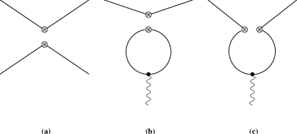
Figure 1:

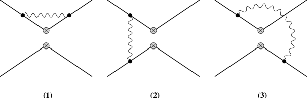
Figure 2:

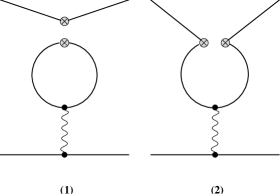
Figure 3:

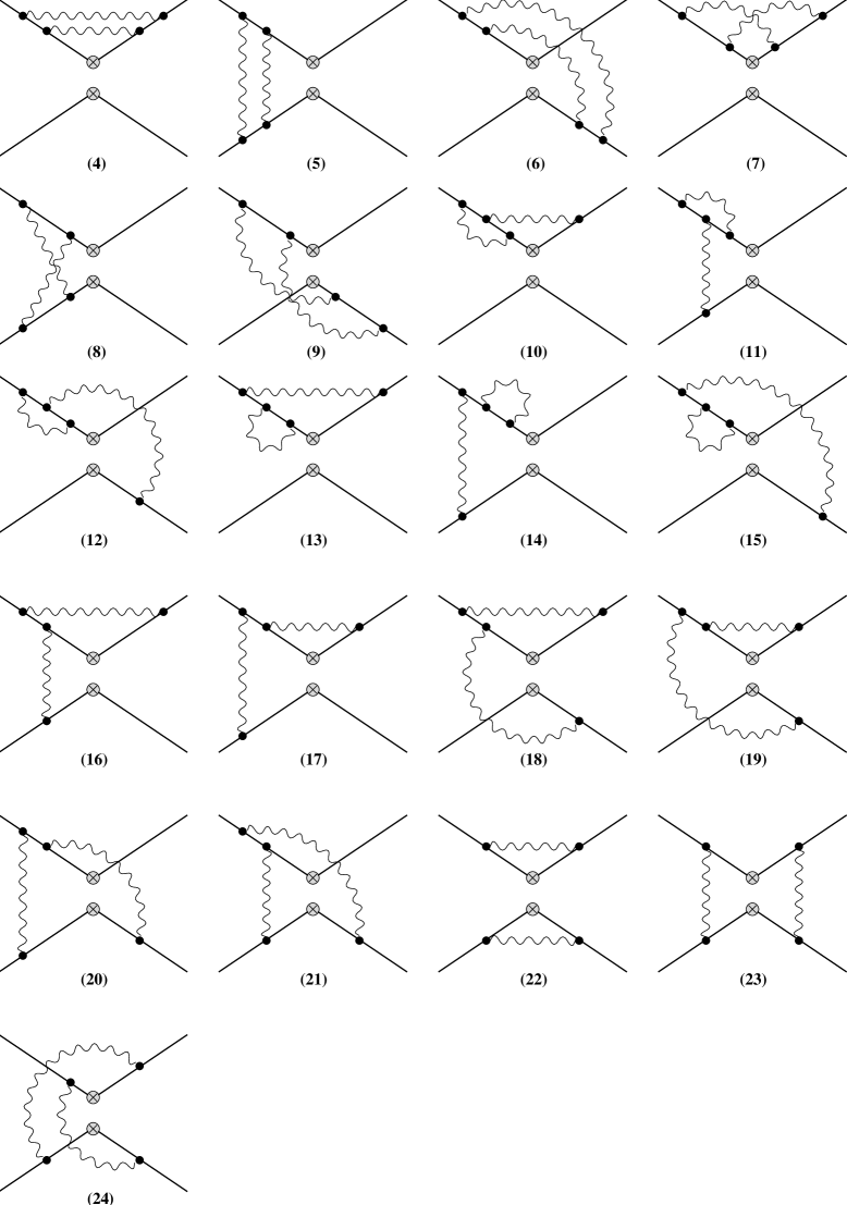
Figure 4:

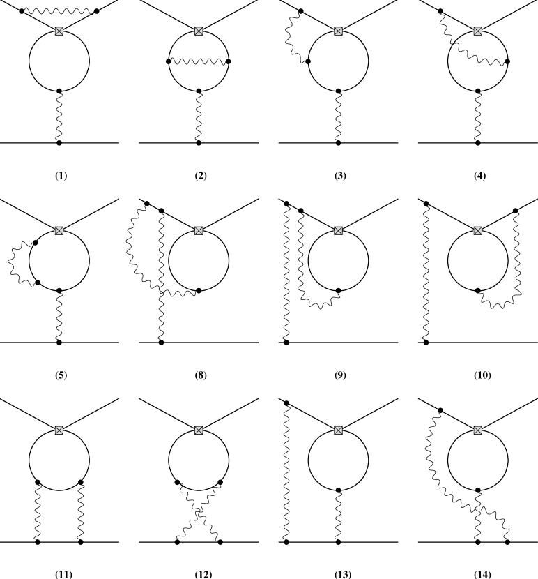
Figure 5:

Figure Captions

Figure 1:

The three basic ways of inserting a given operator into a four–point function: (a) current–current-, (b) type 1 penguin-, (c) type 2 penguin-insertion. The wavy lines denote gluons or photons. The 4-vertices “$\otimes\ \otimes$” denote standard operator insertions.

Figure 2:

One–loop current–current diagrams contributing to $\hat{\gamma}_{\rm e}^{(0)}$. The meaning of lines and vertices is the same as in fig. 1. Possible left-right or up-down reflected diagrams are not shown.

Figure 3:

One–loop type 1 and 2 penguin diagrams contributing to $\hat{\gamma}_{\rm e}^{(0)}$. The meaning of lines and vertices is the same as in fig. 1.

Figure 4:

Two–loop current–current diagrams contributing to $\hat{\gamma}_{\rm se}^{(1)}$. The meaning of lines and vertices is the same as in fig. 1. Possible left-right or up-down reflected diagrams are not shown.

Figure 5:

Two–loop penguin diagrams contributing to $\hat{\gamma}_{\rm se}^{(1)}$. The wavy lines denote gluons or photons. Square-vertices stand for type 1 and 2 penguin insertions as of figs. 1(b) and (c), respectively. Possible left-right reflected diagrams are not shown.

References

- [1] M. K. Gaillard and B. W. Lee, Phys. Rev. Lett. 33 (1974) 108.
- [2] G. Altarelli and L. Maiani, Phys. Lett. 52B (1974) 351.
- [3] A. I. Vainshtein, V. I. Zakharov, and M. A. Shifman, JEPT 45 (1977) 670.
- [4] F. J. Gilman and M. B. Wise, Phys. Rev. D20 (1979) 2392.
- [5] B. Guberina and R. D. Peccei, Nucl. Phys. B163 (1980) 289.
- [6] J. Bijnens and M. B. Wise, Phys. Lett. 137 B (1984) 245.
- [7] A. J. Buras and J.-M. Gérard, Phys. Lett. 192B (1987) 156.
- [8] S. R. Sharpe, Phys. Lett. 194B (1987) 551.
- [9] M. Lusignoli, Nucl. Phys. B325 (1989) 33.
- [10] J. M. Flynn and L. Randall, Phys. Lett. 224B (1989) 221, Erratum 235B (1990) 412.
- [11] G. Buchalla, A. J. Buras, and M. K. Harlander, Nucl. Phys. B337 (1990) 313.
- [12] G. Altarelli, G. Curci, G. Martinelli, and S. Petrarca, Nucl. Phys. B187 (1981) 461.
- [13] A. J. Buras and P. H. Weisz, Nucl. Phys. B333 (1990) 66.
- [14] A. J. Buras, M. Jamin, M. E. Lautenbacher, and P. H. Weisz, Nucl. Phys. B370 (1992) 69; addendum ibid. Nucl. Phys. B375 (1992) 501.
- [15] A. J. Buras, M. Jamin, and M. E. Lautenbacher, Two–Loop Anomalous Dimension Matrix for Weak Non-Leptonic Decays I: , Technical University Munich preprint, TUM-T31-18/92; Max-Planck-Institut preprint, MPI-PAE/PTh 106/92 .
- [16] T. L. Trueman, Phys. Lett. 88B (1979) 331.
- [17] A. Barroso, M. A. Doncheski, H. Grotch, J. G. Körner, and K. Schilcher, Phys. Lett. 261B (1992) 123.
- [18] A. J. Buras, M. Jamin, and M. E. Lautenbacher, Effective Hamiltonians for and Non-Leptonic Decays beyond Leading Logarithms in the Presence of Electroweak Penguins, Technical University Munich preprint, in preparation, TUM-T31-35/92 .