Two–Loop Anomalous Dimension Matrix for
$\Delta S=1$ Weak Non-Leptonic Decays I: ${\cal O}(\alpha_{\rm s}^{2})$

Abstract

We calculate the two–loop $10\times 10$ anomalous dimension matrix ${\cal O}(\alpha_{\rm s}^{2})$ involving current–current operators, QCD penguin operators, and electroweak penguin operators especially relevant for $\Delta S=1$ weak non–leptonic decays, but also important for $\Delta B=1$ decays. The calculation is performed in two schemes for $\gamma_{5}$: the dimensional regularization scheme with anticommuting $\gamma_{5}$ (NDR), and in the ’t Hooft–Veltman scheme. We demonstrate how a direct calculation of diagrams involving $\gamma_{5}$ in closed fermion loops can be avoided thus allowing a consistent calculation in the NDR scheme. The compatibility of the results obtained in the two schemes considered is verified and the properties of the resulting matrices are discussed. The two–loop corrections are found to be substantial. The two–loop anomalous dimension matrix ${\cal O}(\alpha\alpha_{\rm s})$, required for a consistent inclusion of electroweak penguin operators, is presented in a subsequent publication.

1 Introduction

Effective low energy Hamiltonians for non–leptonic weak decays of hadrons are usually written as linear combinations of four–quark operators. The coefficients of these operators, the Wilson coefficient functions, can be calculated in the renormalization group improved perturbation theory, as long as the normalization scale $\mu$ is not too low. The size of these coefficients depends on $\mu$ through the QCD effective coupling constant and on the anomalous dimensions of the operators in question. Since the operators generally mix under renormalization, one deals with anomalous dimension matrices rather than with single anomalous dimensions.

In the case of the $\Delta S=1$ Hamiltonian, relevant for instance for the $\Delta I=1/2$ rule and the ratio $\varepsilon^{\prime}/\varepsilon$, there are ten operators $Q_{i},\;i=1,\ldots,10$ which have to be considered. Consequently one deals with a $10\times 10$ anomalous dimension matrix. The ten operators in question can be divided into three classes:

• current–current operators $Q_{i},\;i=1,2$ originating in the usual W–exchange and subsequent QCD corrections,

• QCD penguin operators $Q_{i},\;i=3,\ldots,6$ originating in QCD penguin diagrams, and

• electroweak penguin operators $Q_{i},\;i=7,\ldots,10$ originating in the photon penguin diagrams.

Explicit expressions for these operators are given in eq. (2.1).

Because of the presence of electroweak penguin operators a consistent analysis must involve anomalous dimensions resulting from both strong and electromagnetic interactions. Working to first order in $\alpha$ but to all orders in $\alpha_{\rm s}$ the following anomalous dimension matrix is needed for the leading and next–to–leading logarithmic approximation for the Wilson coefficient functions,

$$\hat{\gamma}\;=\;\frac{\alpha_{\rm s}}{4\pi}\,\hat{\gamma}_{\rm s}^{(0)}+\frac{\alpha}{4\pi}\,\hat{\gamma}_{\rm e}^{(0)}+\frac{\alpha_{\rm s}^{2}}{(4\pi)^{2}}\,\hat{\gamma}_{\rm s}^{(1)}+\frac{\alpha\alpha_{\rm s}}{(4\pi)^{2}}\,\hat{\gamma}_{\rm se}^{(1)}\;.$$ (1.1)

In the leading logarithmic approximation only the one–loop matrices $\hat{\gamma}_{\rm s}^{(0)}$ and $\hat{\gamma}_{\rm e}^{(0)}$ have to be considered. Inclusion of next–to–leading corrections requires the evaluation of the two–loop matrices $\hat{\gamma}_{\rm s}^{(1)}$ and $\hat{\gamma}_{\rm se}^{(1)}$. In addition some one–loop finite terms are needed.

What is known in the literature are the matrices $\hat{\gamma}_{\rm s}^{(0)}$ and $\hat{\gamma}_{\rm e}^{(0)}$ [1]–[11] and a $2\times 2$ submatrix of $\hat{\gamma}_{\rm s}^{(1)}$ involving the current–current operators $Q_{1}$ and $Q_{2}$ [12, 13]. The purpose of the present and a subsequent paper is to complete the evaluation of the matrix $\hat{\gamma}_{\rm s}^{(1)}$ and to calculate $\hat{\gamma}_{\rm se}^{(1)}$. Together with certain one–loop finite terms this will allow the extension of the phenomenology of non–leptonic $\Delta S=1$ transitions beyond leading logarithms. The results for the $6\times 6$ submatrix of $\hat{\gamma}_{\rm s}^{(1)}$ involving current–current and QCD penguin operators together with some phenomenological implications have already been presented by us in ref. [14]. In the present paper we give the details of these two–loop calculations and generalize them to the full matrix $\hat{\gamma}_{\rm s}^{(1)}$. The matrix $\hat{\gamma}_{\rm se}^{(1)}$ is considered in a subsequent publication [15]. In particular, we present the results for an arbitrary number of colours, $N$, which is useful for the applications of the $1/N$ expansion. The phenomenological implications of these new results will be discussed in ref. [16].

The calculation of the matrices $\hat{\gamma}_{\rm s}^{(1)}$ and $\hat{\gamma}_{\rm se}^{(1)}$ is very tedious. It involves a large number of two–loop diagrams which make the use of an algebraic computer program almost mandatory . Moreover one has to deal with several subtleties which are absent in the calculations of $\hat{\gamma}_{\rm s}^{(0)}$ and $\hat{\gamma}_{\rm e}^{(0)}$. First of all, the two–loop anomalous dimensions depend on the renormalization scheme for operators and the treatment of $\gamma_{5}$ in $D\not=4$ space–time dimensions. It is known for instance on the basis of ref. [13], that the $2\times 2$ submatrix of $\hat{\gamma}_{\rm s}^{(1)}$ involving $Q_{1}$ and $Q_{2}$ calculated in the NDR scheme (naive dimensional regularization with anticommuting $\gamma_{5}$) differs substantially from the one obtained in the HV scheme (non anticommuting $\gamma_{5}$ [19, 20]). The same feature is found for the full matrices $\hat{\gamma}_{\rm s}^{(1)}$ and $\hat{\gamma}_{\rm se}^{(1)}$. The important point is that the difference between $\hat{\gamma}^{(1)}$ calculated in two different schemes is on general grounds entirely given in terms of $\hat{\gamma}^{(0)}$ and the finite parts of one–loop diagrams calculated in the two schemes in question. This relation is very useful for checking the compatibility of two–loop calculations performed in different renormalization schemes and plays an important role in demonstrating the scheme independence of physical quantities. It is given in eq. (2.15). Another subtle point is the dependence of the two–loop anomalous dimensions obtained in the NDR scheme on whether a given operator has been put in colour singlet or colour non–singlet form such as

$$Q_{2}\;=\;\left(\bar{s}_{\alpha}u_{\alpha}\right)_{\rm V-A}\left(\bar{u}_{\beta}d_{\beta}\right)_{\rm V-A}\qquad{\rm or}\qquad\widetilde{Q}_{2}\;=\;\left(\bar{s}_{\alpha}d_{\beta}\right)_{\rm V-A}\left(\bar{u}_{\beta}u_{\alpha}\right)_{\rm V-A}\;.$$ (1.2)

In $D=4$ dimensions $Q_{2}$ and $\widetilde{Q}_{2}$ would be equivalent by means of Fierz transformation. Their one–loop anomalous dimensions are the same.

Again the two–loop anomalous dimensions for these two forms of operators can on general grounds be related to each other by calculating one–loop diagrams. This feature turns out to be fortunate in that it offers one way to deal with dangerous closed fermion loops involving odd numbers of $\gamma_{5}$ in two–loop diagrams. The latter are known to be ambiguous in the case of the NDR scheme. Indeed, as we will demonstrate explicitly in section 5 and in ref. [15], it is possible by using different forms of the operators and the relation mentioned above, to express all diagrams with closed fermion loops in terms of diagrams not containing such loops. In this way, consistent calculations of $\hat{\gamma}_{\rm s}^{(1)}$ and $\hat{\gamma}_{\rm se}^{(1)}$ can be performed in the NDR scheme and compared with the one obtained in the HV scheme, free of $\gamma_{5}$ problems.

The following sections constitute the calculation of $\hat{\gamma}_{\rm s}^{(1)}$ and a detailed discussion of the subtle points mentioned above. In ref. [15], the methods developed here are generalized to include photon exchanges and are used to calculate $\hat{\gamma}_{\rm se}^{(1)}$.

Our paper is organized as follows: In section 2, we give a list of the ten operators in question, and we classify the one and two–loop diagrams into current–current and penguin diagrams. We also discuss the basic formalism necessary for the calculation of $\hat{\gamma}_{\rm s}^{(1)}$. In section 3, we recall the matrix $\hat{\gamma}_{\rm s}^{(0)}$, and we calculate the finite terms of one–loop diagrams in the NDR and HV scheme. In section 4, the calculations and results for two–loop current–current diagrams are presented. In section 5, an analogous presentation is given for two–loop penguin diagrams. In section 6, we combine the results of the previous sections to obtain $\hat{\gamma}_{\rm s}^{(1)}$ in NDR and HV schemes. We discuss various properties of this matrix, in particular its Large-$N$ limit. Section 7 contains a brief summary of our paper. In appendices A and B explicit expressions for the elements of the $10\times 10$ matrices $\hat{\gamma}_{\rm s}^{(0)}$ and $\hat{\gamma}_{\rm s}^{(1)}$ for an arbitrary number of colours ($N$) and flavours ($f$) are given. In appendix C the corresponding results for $\hat{\gamma}_{\rm s}^{(1)}$ in the case of $N=3$ are presented.

2 General Formalism

2.1 Operators

The ten operators considered in this paper are given as follows

$$Q_{1} = \left(\bar{s}_{\alpha}u_{\beta}\right)_{\rm V-A}\left(\bar{u}_{\beta}d_{\alpha}\right)_{\rm V-A}\,,$$

$$Q_{2} = \left(\bar{s}u\right)_{\rm V-A}\left(\bar{u}d\right)_{\rm V-A}\,,$$

$$Q_{3} = \left(\bar{s}d\right)_{\rm V-A}\sum_{q}\left(\bar{q}q\right)_{\rm V-A}\,,$$

$$Q_{4} = \left(\bar{s}_{\alpha}d_{\beta}\right)_{\rm V-A}\sum_{q}\left(\bar{q}_{\beta}q_{\alpha}\right)_{\rm V-A}\,,$$

$$Q_{5} = \left(\bar{s}d\right)_{\rm V-A}\sum_{q}\left(\bar{q}q\right)_{\rm V+A}\,,$$

$$Q_{6} = \left(\bar{s}_{\alpha}d_{\beta}\right)_{\rm V-A}\sum_{q}\left(\bar{q}_{\beta}q_{\alpha}\right)_{\rm V+A}\,,$$ (2.1)

$$Q_{7} = \frac{3}{2}\left(\bar{s}d\right)_{\rm V-A}\sum_{q}e_{q}\left(\bar{q}q\right)_{\rm V+A}\,,$$

$$Q_{8} = \frac{3}{2}\left(\bar{s}_{\alpha}d_{\beta}\right)_{\rm V-A}\sum_{q}e_{q}\left(\bar{q}_{\beta}q_{\alpha}\right)_{\rm V+A}\,,$$

$$Q_{9} = \frac{3}{2}\left(\bar{s}d\right)_{\rm V-A}\sum_{q}e_{q}\left(\bar{q}q\right)_{\rm V-A}\,,$$

$$Q_{10} = \frac{3}{2}\left(\bar{s}_{\alpha}d_{\beta}\right)_{\rm V-A}\sum_{q}e_{q}\left(\bar{q}_{\beta}q_{\alpha}\right)_{\rm V-A}\,,$$

where $\alpha$, $\beta$ denote colour indices ($\alpha,\beta=1,\ldots,N$) and $e_{q}$ are quark charges. We have omitted colour indices for the colour singlet operators. $(V\pm A)$ refers to $\gamma_{\mu}(1\pm\gamma_{5})$. This basis closes under QCD and QED renormalization and is complete if external momenta and masses are neglected. However, at intermediate stages of the calculation, we have to retain operators which vanish on–shell. This will be discussed in detail in section 5.2.

At one place, it will become useful to study a second basis in which the first two operators are replaced by their Fierz conjugates,

$$\widetilde{Q}_{1} = \left(\bar{s}d\right)_{\rm V-A}\left(\bar{u}u\right)_{\rm V-A}\,,$$

$$\widetilde{Q}_{2} = \left(\bar{s}_{\alpha}d_{\beta}\right)_{\rm V-A}\left(\bar{u}_{\beta}u_{\alpha}\right)_{\rm V-A}\,,$$ (2.2)

with the remaining operators unchanged. In fact, the latter basis is the one used by Gilman and Wise [4]. We prefer however to put $Q_{2}$ in the colour singlet form as in eq. (2.1), because it is this form in which the operator $Q_{2}$ enters the tree level Hamiltonian. Let us finally recall that the Fierz conjugates of the $(V-A)\otimes(V+A)$ operators $Q_{6}$ and $Q_{8}$ are given by

$$\widetilde{Q}_{6} = -\,8\sum_{q}\left(\bar{s}_{\rm L}q_{\rm R}\right)\left(\bar{q}_{\rm R}d_{\rm L}\right)\,,$$

$$\widetilde{Q}_{8} = -\,12\sum_{q}e_{q}\left(\bar{s}_{\rm L}q_{\rm R}\right)\left(\bar{q}_{\rm R}d_{\rm L}\right)\,,$$ (2.3)

with similar expressions for $\widetilde{Q}_{5}$ and $\widetilde{Q}_{7}$. Here $q_{R,L}=\frac{1}{2}(1\pm\gamma_{5})q$. The Fierz conjugates of the $(V-A)\otimes(V-A)$ penguin operators $Q_{3},Q_{4},Q_{9}$ and $Q_{10}$, to be denoted by $\widetilde{Q}_{i},\;i=3,4,9,10$, can be found in analogy to (2.2).

2.2 Classification of Diagrams

In order to calculate the anomalous dimension matrices $\hat{\gamma}_{\rm s}^{(0)}$ and $\hat{\gamma}_{\rm s}^{(1)}$, one has to insert the operators of eq. (2.1) in appropriate four–point functions and extract $1/\varepsilon$ divergences. The precise relation between the $1/\varepsilon$ divergences in one– and two–loop diagrams and the one– and two–loop anomalous dimension matrices will be given in the following subsection. Here, let us only recall that insertion of any of the operators of eq. (2.1) into the diagrams discussed below results in a linear combination of the operators $Q_{i}$. A row in the anomalous dimension matrix corresponding to the inserted operator can then be obtained from the coefficients in the linear combination in question.

There are three basic ways a given operator can be inserted into a four–point function. They are shown in fig. 1, where the cross denotes the interaction described by a current in a given operator of eq. (2.1), and the wavy line denotes a gluon. We shall refer to the insertions of fig. 1(a) as “current–current” insertions. The insertions of fig. 1(b) and (c) will then be called “penguin insertions” of type 1 and type 2 respectively.

The complete list of the diagrams necessary for one– and two–loop calculations is given in figs. 2–7. At the one–loop level one has three current–current diagrams, fig. 2, to be denoted as in ref. [13] by $D_{1}$ – $D_{3}$ and one penguin diagram of each type, fig. 3, to be denoted by $P_{0}^{(1)}$ and $P_{0}^{(2)}$ for type 1 and type 2 insertion respectively. At the two–loop level there are 28 current–current diagrams shown in fig. 4, to be denoted by $D_{4}$ – $D_{31}$, and 14 penguin diagrams of each type shown in fig. 5, to be denoted by $P_{1}^{(1)}$ – $P_{14}^{(1)}$ and $P_{1}^{(2)}$ – $P_{14}^{(2)}$ respectively. The diagrams obtained from the ones given here by left-right reflections have not been shown. In the case of current–current diagrams also up-down reflections have to be considered. In fig. 6, we show two penguin diagrams which have no $1/\varepsilon$ divergence and hence do not contribute to the anomalous dimensions, and in fig. 7, some examples of penguin diagrams which vanish identically in dimensional regularization are given.

2.3 Basic Formulae for the Anomalous Dimensions

The anomalous dimensions of the operators $Q_{i}$, calculated in the $\overline{MS}$ scheme, are obtained from the $1/\varepsilon$ divergences of the diagrams of figs. 2 – 5 and from the $1/\varepsilon$ divergence of the quark wave function renormalization. Let us denote by $\vec{Q}$ a column vector composed of the operators $Q_{i}$. Then

$$\hat{\gamma}(g)\;=\;\hat{Z}^{-1}\,\mu\,\frac{d}{d\mu}\,\hat{Z},\qquad{\rm with}\qquad\vec{Q}^{B}\;=\;\hat{Z}\,\vec{Q}\,,$$ (2.4)

where $\vec{Q}^{B}$ stands for bare operators. Working in $D=4-2\,\varepsilon$ dimensions, we can expand $\hat{Z}$ in inverse powers of $\varepsilon$ as follows

$$\hat{Z}\;=\;\hat{1}+\sum_{k=1}^{\infty}\frac{1}{\varepsilon^{k}}\,\hat{Z}_{k}(g)\,.$$ (2.5)

where $g$ is the QCD coupling constant. Inserting (2.5) into (2.4) one derives a useful formula

$$\hat{\gamma}(g)\;=\;-\,2\,g^{2}\,\frac{\partial\hat{Z}_{1}(g)}{\partial g^{2}}\,.$$ (2.6)

Let us next denote by $\Gamma^{(4)}(\vec{Q})$ and $\Gamma_{B}^{(4)}(\vec{Q}^{B})$ the renormalized and the bare four–quark Green functions with operator $\vec{Q}$ insertions. Strictly speaking $\Gamma^{(4)}(\vec{Q})$ and $\Gamma_{B}^{(4)}(\vec{Q}^{B})$ are matrices, because the insertion of a single operator in a given diagram results in a linear combination of operators.

At the one–loop level $\Gamma_{B}^{(4)}$ is obtained by evaluating the diagrams of figs. 2 and 3. At the two–loop level it is found by evaluating the diagrams of figs. 4 and 5 and subtracting the corresponding two–loop counter terms. For the results of tabs. 1 – 4, we have made these subtractions diagram by diagram. Next

$$\Gamma^{(4)}(\vec{Q})\;=\;\hat{Z}_{\psi}\hat{Z}^{-1}\,\Gamma_{B}^{(4)}(\vec{Q}^{B})\,,$$ (2.7)

where $\hat{Z}_{\psi}$ is a matrix which represents the renormalization of the four quark fields. In the case of pure QCD it is a diagonal matrix with all the diagonal elements being equal to $Z^{{(\psi)}^{2}}$, where $Z^{(\psi)}$ is the quark wave function renormalization, defined by

$$\psi^{B}\;=\;{Z^{(\psi)}}^{1/2}\,\psi\,.$$ (2.8)

We expand $\Gamma_{B}^{(4)}$ and $Z^{(\psi)}$ in inverse powers of $\varepsilon$ as follows

$$Z^{(\psi)} = 1+\sum_{k=1}^{\infty}\frac{1}{\varepsilon^{k}}\,Z^{(\psi)}_{k}(g)\,,$$ (2.9)

$$\Gamma_{B}^{(4)}(Q_{i}) = \hat{1}+\sum_{k=1}^{\infty}\frac{1}{\varepsilon^{k}}\,Z^{(\Gamma)}_{k}(g,Q_{i})\;+\;{\rm finite}\,,$$ (2.10)

where

$$Z^{(\psi)}_{1}(g)\;=\;a_{1}\,\frac{g^{2}}{16\pi^{2}}+a_{2}\,\frac{g^{4}}{(16\pi^{2})^{2}}+{\cal O}(g^{6})\,,$$ (2.11)

and

$$Z^{(\Gamma)}_{1}(g,Q_{i})\;=\;\sum_{j=1}^{10}\left[\,\left(b_{1}\right)_{ij}\frac{g^{2}}{16\pi^{2}}+\left(b_{2}\right)_{ij}\frac{g^{4}}{(16\pi^{2})^{2}}+{\cal O}(g^{6})\,\right]\;.$$ (2.12)

Demanding $\Gamma^{(4)}$ to be finite, we find $\hat{Z}_{1}$, and, using (2.6), the basic formulae for the one– and two–loop anomalous dimension matrices,

$$\big{(}\hat{\gamma}_{\rm s}^{(0)}\big{)}_{ij} = -\,2\left[\,2\,a_{1}\,\delta_{ij}+\left(b_{1}\right)_{ij}\,\right]\,,$$ (2.13)

$$\big{(}\hat{\gamma}_{\rm s}^{(1)}\big{)}_{ij} = -\,4\left[\,2\,a_{2}\,\delta_{ij}+\left(b_{2}\right)_{ij}\,\right]\,.$$ (2.14)

2.4 Renormalization Scheme Dependence of $\hat{\gamma}_{\rm s}^{(1)}$

The two–loop anomalous dimension matrices depend on the renormalization scheme and in particular on the treatment of $\gamma_{5}$ in $D\not=4$ dimensions. In ref. [14], we have derived a relation between $(\hat{\gamma}_{\rm s}^{(1)})_{a}$ and $(\hat{\gamma}_{\rm s}^{(1)})_{b}$ calculated in two different renormalization schemes $a$ and $b$,

$$\big{(}\hat{\gamma}_{\rm s}^{(1)}\big{)}_{b}\;=\;\big{(}\hat{\gamma}_{\rm s}^{(1)}\big{)}_{a}+\left[\Delta\hat{r}_{\rm s},\hat{\gamma}_{\rm s}^{(0)}\right]+2\,\beta_{0}\Delta\hat{r}_{\rm s}\qquad{\rm with}\qquad\Delta\hat{r}_{\rm s}\;=\;(\hat{r}_{\rm s})_{b}-(\hat{r}_{\rm s})_{a}\,,$$ (2.15)

where $\beta_{0}$ is the leading coefficient in the expansion of the $\beta$–function

$$\beta(g)\;=\;-\,\beta_{0}\,\frac{g^{3}}{16\pi^{2}}-\beta_{1}\,\frac{g^{5}}{(16\pi^{2})^{2}}-\cdots\,,$$ (2.16)

and the $(\hat{r}_{\rm s})_{i}$ are defined by

$$\langle\vec{Q}\rangle_{i}\;=\;\left[\,\hat{\bf 1}+\frac{g^{2}}{16\pi^{2}}\,(\hat{r}_{\rm s})_{i}\,\right]\langle\vec{Q}^{(0)}\rangle\;.$$ (2.17)

Here, $\vec{Q}^{(0)}$ is a tree–level matrix element and $\langle\vec{Q}\rangle_{i}$ denotes renormalized one–loop matrix elements calculated in the scheme $i$. The matrices $(\hat{r}_{\rm s})_{i}$ are obtained by calculating the finite terms in the one–loop diagrams of figs. 2 and 3.

Relation (2.15) is very useful as it allows to test compatibility of the two–loop anomalous dimension matrices calculated in two different renormalization schemes. It also plays a central role in demonstrating the scheme independence of physical quantities [14].

2.5 Collection of Useful Results

Let us recall the values for $\beta_{0}$, $\beta_{1}$, $a_{1}$, and $a_{2}$,

$$\beta_{0}\;=\;\frac{11}{3}N-\frac{2}{3}f\,,\qquad\qquad\beta_{1}\;=\;\frac{34}{3}N^{2}-\frac{10}{3}Nf-2\,C_{F}f\,,$$ (2.18)

$$a_{1}\;=\;-\,C_{F}\,,\qquad\qquad a_{2}\;=\;C_{F}\left[\,\frac{3}{4}\,C_{F}-\frac{17}{4}N+\frac{1}{2}f\,\right]\,,$$ (2.19)

where $C_{F}=(N^{2}-1)/2N$. Here, $N$ is the number of colours and $f$ the number of active flavours. All four quantities in eqs. (2.18) and (2.19) are common to the NDR and HV scheme. Moreover $\beta_{0}$ and $\beta_{1}$ are gauge independent. The coefficients $a_{1}$ and $a_{2}$ given here correspond to the Feynman gauge.

In the course of the discussion of the anomalous dimensions of the penguin operators $Q_{6}$ and $Q_{8}$ it will be useful to have at hand the anomalous dimension of the mass operator $\bar{\psi}\psi$,

$$\gamma_{m}\;=\;\gamma_{m}^{(0)}\,\frac{g^{2}}{16\pi^{2}}+\gamma_{m}^{(1)}\,\frac{g^{4}}{(16\pi^{2})^{2}}+\cdots\,.$$ (2.20)

To two loops, the anomalous dimensions $\gamma_{m}^{(0)}$ and $\gamma_{m}^{(1)}$ are given by

$$\gamma_{m}^{(0)}\;=\;-\,6\,C_{F}\qquad{\rm and}\qquad\gamma_{m}^{(1)}\;=\;-\,C_{F}\left[\,3\ C_{F}+\frac{97}{3}N-\frac{10}{3}f\,\right]\,,$$ (2.21)

for both schemes [21].

Finally let us recall that for the anomalous dimension of the weak current,

$$\gamma_{J}\;=\;\gamma_{J}^{(0)}\frac{g^{2}}{16\pi^{2}}+\gamma_{J}^{(1)}\frac{g^{4}}{(16\pi^{2})^{2}}+\cdots\,.$$ (2.22)

the one-loop coefficient $\gamma_{J}^{(0)}$ vanishes in both schemes. However, at the two–loop level in the HV scheme, $\gamma_{J}^{(1)}$ is found to be non–vanishing [13],

$$\gamma_{J}^{(1)}\;=\;\left\{\begin{array}[]{ll}0&\qquad{\rm NDR}\\ 4\,\beta_{0}\,C_{F}&\qquad{\rm HV}\end{array}\right.\,.$$ (2.23)

In the HV scheme the axial current attains a finite renormalization if one subtracts minimally, as we did, and one gets a mixing between chiral components. This is not so aesthetic and on hindsight it would have been more elegant to redefine the currents non-minimally to retain standard normalization. We do not proceed along this line but in our computation the mixing reappears in the non-vanishing of the two–loop coefficient $\gamma_{J}^{(1)}$. However, since the one-loop matrix elements $\hat{r}$ also change correspondingly, the final physical quantities are normalized properly and scheme independent in the end.

3 One–Loop Results

3.1 Current–Current Contributions to $\hat{\gamma}_{\rm s}^{(0)}$

The contributions of diagrams $D_{1}$ – $D_{3}$ of fig. 2 to the matrix $\hat{\gamma}_{\rm s}^{(0)}$ have a very simple structure. The mixing between different operators can be divided into five blocks, each containing two operators,

$$\left(Q_{k},Q_{k+1}\right)\,,\qquad\qquad k=1,3,5,7,9\,,$$ (3.1)

with no mixing between different blocks. Moreover, the mixing among $(V-A)\otimes(V-A)$ operators $(k=1,3,9)$ is described by a universal $2\times 2$ matrix. Using eq. (2.13), one finds

$$\left[\hat{\gamma}_{\rm s}^{(0)}(Q_{1},Q_{2})\right]_{\rm cc}\;=\;\left(\begin{array}[]{cc}-\,6/N&6\\ 6&-\,6/N\end{array}\right)\,,$$ (3.2)

with identical results for $(Q_{3},Q_{4})$ and $(Q_{9},Q_{10})$.

Similarly,

$$\left[\hat{\gamma}_{\rm s}^{(0)}(Q_{5},Q_{6})\right]_{\rm cc}\;=\;\left(\begin{array}[]{cc}6/N&-\,6\\ 0&-\,6\,(N^{2}-1)/N\end{array}\right)\,,$$ (3.3)

with identical result for $(Q_{7},Q_{8})$.

Comparing with eq. (2.21), we note that

$$\left[\gamma_{66}^{(0)}\right]_{\rm cc}\;=\;\left[\gamma_{88}^{(0)}\right]_{\rm cc}\;=\;2\,\gamma_{m}^{(0)}\,,$$ (3.4)

showing that the one–loop anomalous dimensions of the operators $Q_{6}$ and $Q_{8}$ are twice the one–loop anomalous dimension of the mass operator, provided only current–current diagrams $D_{1}$ – $D_{3}$ are taken into account. It should be pointed out that this result is valid for an arbitrary number of colours $N$, but remains only true in the Large-$N$ limit when penguin insertions are taken into account [22, 23].

3.2 Penguin Contributions to $\hat{\gamma}_{\rm s}^{(0)}$

The contributions of the diagrams $P_{0}^{(1)}$ and $P_{0}^{(2)}$ of fig. 3 to the matrix $\hat{\gamma}_{\rm s}^{(0)}$ have also a very simple structure:

• The insertions of $Q_{1}$, $Q_{5}$, and $Q_{7}$ into the diagrams $P_{0}^{(1)}$ and $P_{0}^{(2)}$ vanish. This follows either from colour conservation, or flavour conservation, or finally from the Dirac structure, as one can easily verify by inspecting the diagrams of fig. 3. Thus, the corresponding rows in $\left[\hat{\gamma}_{\rm s}^{(0)}\right]_{\rm p}$ vanish,

  $$\left[\hat{\gamma}_{\rm s}^{(0)}(Q_{1})\right]_{\rm p}\;=\;\left[\hat{\gamma}_{\rm s}^{(0)}(Q_{5})\right]_{\rm p}\;=\;\left[\hat{\gamma}_{\rm s}^{(0)}(Q_{7})\right]_{\rm p}\;=\;0\,.$$ (3.5)

• The insertion of any of the remaining operators into the diagrams of fig. 3 results always into a unique linear combination of the QCD penguin operators $Q_{3}$ – $Q_{6}$, multiplied by an overall factor characteristic for the inserted operator. Denoting by

  $$P\;=\;\left(0,\,0,\,-\,\frac{1}{N},\,1,\,-\,\frac{1}{N},\,1,\,0,\,0,\,0,\,0\right)$$ (3.6)

  the row vector in the space ($Q_{1}$ – $Q_{10}$), the non-vanishing elements of $\hat{\gamma}_{\rm s}^{(0)}$, coming from the diagrams of fig. 3, are as follows,

  $$\begin{array}[]{rclrcl}\left[\hat{\gamma}_{\rm s}^{(0)}(Q_{2})\right]_{\rm p}&=&\frac{2}{3}\,P\,,&\left[\hat{\gamma}_{\rm s}^{(0)}(Q_{3})\right]_{\rm p}&=&\phantom{-}\,\frac{4}{3}\,P\,,\\ \left[\hat{\gamma}_{\rm s}^{(0)}(Q_{4})\right]_{\rm p}&=&\frac{2}{3}\,fP\,,&\left[\hat{\gamma}_{\rm s}^{(0)}(Q_{6})\right]_{\rm p}&=&\phantom{-}\,\frac{2}{3}\,fP\,,\\ \left[\hat{\gamma}_{\rm s}^{(0)}(Q_{8})\right]_{\rm p}&=&\frac{2}{3}\big{(}u-\frac{d}{2}\big{)}\,P\,,&\left[\hat{\gamma}_{\rm s}^{(0)}(Q_{9})\right]_{\rm p}&=&-\,\frac{2}{3}\,P\,,\\ \left[\hat{\gamma}_{\rm s}^{(0)}(Q_{10})\right]_{\rm p}&=&\frac{2}{3}\big{(}u-\frac{d}{2}\big{)}\,P\,,&&&\end{array}$$ (3.7)

  where $u$ and $d$ denote the number of up– and down–quark flavours respectively ($u+d=f$). In obtaining (3.7), eq. (2.13) has been used with $a_{1}$ omitted, since this contribution has already been included in (3.2) and (3.3).

Combining the results of eqs. (3.2), (3.3), (3.5), and (3.7), we find the known complete one–loop anomalous dimension matrix $\hat{\gamma}_{\rm s}^{(0)}$. For completeness this matrix has been given explicitly in appendix A.

It should be stressed, that these results do not depend on the renormalization scheme for $Q_{i}$ and are also valid for $\widetilde{Q}_{i}$. This is no longer the case for the finite terms in the diagrams of figs. 2 and 3, to which we now turn our attention.

3.3 Current–Current Contributions to $\Delta\hat{r}_{\rm s}$

The contribution to the matrix $\hat{r}_{\rm s}$ defined in eq. (2.17), resulting from the diagrams $D_{1}$ – $D_{3}$ of fig. 2.

• depends on the renormalization scheme for $Q_{i}$, but

• does not depend on whether $Q_{i}$, or their Fierz conjugates $\widetilde{Q}_{i}$, are inserted in these diagrams.

The general structure of $\left[\hat{r}_{\rm s}\right]_{\rm cc}$ is the same as in the case of $\left[\hat{\gamma}_{\rm s}^{(0)}\right]_{\rm cc}$ presented in section 3.1.

Since $\hat{r}$ is generally gauge dependent and dependent on the infrared structure of the theory we give here only results for

$$\Delta\hat{r}_{\rm s}\equiv\hat{r}_{\rm s,HV}-\hat{r}_{\rm s,NDR}$$ (3.8)

which are free from these dependences. The results for $\hat{r}_{\rm s}$ in the Landau–gauge have been given in ref. [14].

We find

$$\left[\Delta\hat{r}_{\rm s}(Q_{1},Q_{2})\right]_{\rm cc}\;=\;\left(\begin{array}[]{cc}2N-4/N&2\\ 2&2N-4/N\end{array}\right)\,,$$ (3.9)

with identical results for $(Q_{3},Q_{4})$ and $(Q_{9},Q_{10})$. Similarly,

$$\left[\Delta\hat{r}_{\rm s}(Q_{5},Q_{6})\right]_{\rm cc}\;=\;\left(\begin{array}[]{cc}2N-8/N&6\\ 4&4N-8/N\end{array}\right)\,,$$ (3.10)

with identical result for $(Q_{7},Q_{8})$.

3.4 Penguin Contributions to $\Delta\hat{r}_{\rm s}$

Turning our attention to the finite parts of the penguin diagrams of fig. 3, it should be first noted that at the one loop level one does not face the problem of the evaluation of ${\rm Tr}[\gamma_{5}\gamma_{\mu}\gamma_{\nu}\gamma_{\lambda}\gamma_{\omega}]$ in $D\not=4$ dimensions. Consequently, the diagram $P_{0}^{(1)}$ can be calculated in the NDR renormalization scheme without any difficulties. Nevertheless, different results are obtained for the NDR and HV scheme.

The reason that no problem with closed fermion loops arises at this level is as follows. Although at the intermediate state ${\rm Tr}(\gamma_{\tau}\gamma_{5}\gamma_{\nu}\gamma_{\lambda}\gamma_{\mu})$ appears it is contracted with $g_{\mu\nu}$ and $q_{\mu}q_{\nu}$ where $q$ is the momentum of the gluon. Thus actually only the trace ${\rm Tr}(\gamma_{\tau}\gamma_{5}\gamma_{\lambda})$ has to be calculated, which however is zero.

The structure of the results is similar to the ones given in section 3.2. In addition to the above mentioned scheme dependence, in the case of the NDR, but not the HV scheme, the results for the insertions of the operators $Q_{2}$, $Q_{3}$, $Q_{4}$, $Q_{9}$, and $Q_{10}$ depend on whether these operators are taken in the basic form of eq. (2.1) or in the Fierz conjugate form $\widetilde{Q}_{i}$. In the case of pure QCD corrections the results for $Q_{1}$, and for the $(V-A)\otimes(V+A)$ operators $Q_{5}$ – $Q_{8}$, do not depend on the form used. These properties will play an important role in section 5.

Beginning with the basis of eq. (2.1), we find that the insertions of $Q_{1}$, $Q_{5}$, and $Q_{7}$ into the diagrams $P_{0}^{(1)}$ and $P_{0}^{(2)}$ vanish in both renormalization schemes considered. Thus the corresponding rows in $\left[\hat{r}_{\rm s,NDR}\right]_{\rm p}$ and $\left[\hat{r}_{\rm s,HV}\right]_{\rm p}$ vanish,

$$\left[\hat{r}_{\rm s,NDR}(Q_{1})\right]_{\rm p}\;=\;\left[\hat{r}_{\rm s,NDR}(Q_{5})\right]_{\rm p}\;=\;\left[\hat{r}_{\rm s,NDR}(Q_{7})\right]_{\rm p}\;=\;0\,,$$ (3.11)

with an identical result for HV scheme.

The remaining insertions are non-zero but $\left[\Delta\hat{r}_{\rm s}\right]_{\rm p}$ turns out to vanish for $Q_{4}$, $Q_{6}$, $Q_{8}$ and $Q_{10}$:

$$\left[\Delta\hat{r}_{\rm s}(Q_{4})\right]_{\rm p}\;=\;\left[\Delta\hat{r}_{\rm s}(Q_{6})\right]_{\rm p}\;=\;\left[\Delta\hat{r}_{\rm s}(Q_{8})\right]_{\rm p}\;=\;\left[\Delta\hat{r}_{\rm s}(Q_{10})\right]_{\rm p}\;=\;0\,.$$ (3.12)

For the remaining operators we find then

$$\begin{array}[]{rcl}\left[\Delta\hat{r}_{\rm s}(Q_{2})\right]_{\rm p}&=&-\,\frac{1}{3}\,P\,,\\ \left[\Delta\hat{r}_{\rm s}(Q_{3})\right]_{\rm p}&=&-\,\frac{2}{3}\,P\,,\\ \left[\Delta\hat{r}_{\rm s}(Q_{9})\right]_{\rm p}&=&\phantom{-}\,\frac{1}{3}\,P\,,\end{array}$$ (3.13)

where the vector $P$ has been defined in (3.6).

Since, as stated above, $Q_{2}$ and $\tilde{Q}_{2}$ insertions give different results in the NDR scheme, we find that the $\hat{r}_{\rm s,NDR}$ calculated in the bases (2.1) and (2.2) differ. One obtains

$$\widetilde{\Delta}\hat{r}_{\rm s,NDR}\;\equiv\;\hat{r}_{\rm s,NDR}[\ref{eq:2.2}]-\hat{r}_{\rm s,NDR}[\ref{eq:2.1}]\;=\;\left(\begin{array}[]{c}0\\ -\frac{1}{3}P\\ 0\\ \vdots\\ 0\end{array}\right)\,.$$ (3.14)

This result will play an important role in section 5.

4 Current–Current Contributions to the Two–Loop Anomalous Dimension Matrix

4.1 $(V-A)\otimes(V-A)$ Operators

The generalization of the one–loop matrix of eq. (3.2) to two–loop level can be done using the results of ref. [13], where the eigenvalues of the $2\times 2$ submatrix $(Q_{1},Q_{2})$ have been calculated in the NDR and HV schemes. Since also at two–loop level the corresponding submatrix is symmetric with equal entries on the diagonal, one has

$$\left[\gamma_{11}^{(1)}\right]_{\rm cc}= \left[\gamma_{22}^{(1)}\right]_{\rm cc}= \frac{1}{2}\Big{(}\,\tilde{\gamma}{+}^{(1)}+\tilde{\gamma}{-}^{(1)}\,\Big{)}+2\,\gamma_{J}^{(1)}\,,$$ (4.1)

$$\left[\gamma_{12}^{(1)}\right]_{\rm cc}= \left[\gamma_{21}^{(1)}\right]_{\rm cc}= \frac{1}{2}\Big{(}\,\tilde{\gamma}{+}^{(1)}-\tilde{\gamma}{-}^{(1)}\,\Big{)}\,,$$ (4.2)

with $\tilde{\gamma}{\pm}^{(1)}$ given by formulae (5.2) and (5.3) of ref. [13] for NDR and HV schemes respectively, and $\gamma_{J}^{(1)}$ in (2.23) of the present paper.

The details of the calculation of the diagrams $D_{4}$ – $D_{31}$ of fig. 4, with $(V-A)\otimes(V-A)$ insertions, can be found in ref. [13], where a table of $1/\varepsilon^{2}$ and $1/\varepsilon$ singularities in the diagrams $D_{4}$ – $D_{31}$ has been given. In performing these calculations one has to take care of evanescent operators which, although vanishing in $D=4$, affect the two–loop anomalous dimension matrix of physical operators $Q_{i}$ of eq. (2.1). For this reason, the treatment of counter diagrams has to be done with care. The discussion of evanescent operators can be found in ref. [13], and a nice presentation is given also in [24]. Here it suffices to give only the projections on the space of physical operators. Denoting the evanescent operators generally by $E_{\alpha\beta,\gamma\delta}$, with $\alpha$, $\beta$, $\gamma$, $\delta$ being Dirac indices, the relevant projection for diagrams involving $(V-A)\otimes(V-A)$ operators used in ref. [13] is given by

$$E_{\alpha\beta,\gamma\delta}\;\big{(}\gamma_{\tau}(1+\gamma_{5})\big{)}_{\beta\gamma}\,\big{(}\gamma^{\tau}(1+\gamma_{5})\big{)}_{\delta\alpha}\;=\;0\,,$$ (4.3)

where in the HV scheme $\gamma_{\tau}$ has to be taken in $D=4$.

Using eqs. (4.1) and (4.2), together with the results of ref. [13], we find in the case of the NDR scheme

$$\left[\hat{\gamma}_{\rm s,NDR}^{(1)}(Q_{1},Q_{2})\right]_{\rm cc}\;=\;\left(\begin{array}[]{cc}A_{\rm NDR}&B_{\rm NDR}\\ B_{\rm NDR}&A_{\rm NDR}\end{array}\right)\,,$$ (4.4)

where

$$A_{\rm NDR}\;=\;-\,\frac{22}{3}-\frac{2}{3}\frac{f}{N}-\frac{57}{2}\frac{1}{N^{2}}\,,\qquad B_{\rm NDR}\;=\;-\,\frac{19}{6}N+\frac{2}{3}f+\frac{39}{N}\,,$$ (4.5)

with identical results for $(Q_{3},Q_{4})$ and $(Q_{9},Q_{10})$.

For the HV scheme we find

$$\left[\hat{\gamma}_{\rm s}^{(1)}(Q_{1},Q_{2})\right]_{\rm cc}\;=\;\left(\begin{array}[]{cc}A_{\rm HV}&B_{\rm HV}\\ B_{\rm HV}&A_{\rm HV}\end{array}\right)\,,$$ (4.6)

where

$$A_{\rm HV}\;=\;\frac{44}{3}N^{2}-\frac{8}{3}Nf-\frac{110}{3}+\frac{14}{3}\frac{f}{N}-\frac{57}{2}\frac{1}{N^{2}}\,,\qquad B_{\rm HV}\;=\;\frac{23}{2}N-2f+\frac{39}{N}\,,$$ (4.7)

with identical results for $(Q_{3},Q_{4})$ and $(Q_{9},Q_{10})$.

4.2 $(V-A)\otimes(V+A)$ Operators

The calculation of the $(V-A)\otimes(V+A)$ insertions into the diagrams $D_{4}$ – $D_{31}$ proceeds in analogy with the one for $(V-A)\otimes(V-A)$ operators. However, the projection on the space of physical operators takes this time the following form,

$$E_{\alpha\beta,\gamma\delta}\;(1-\gamma_{5})_{\beta\gamma}\,(1+\gamma_{5})_{\delta\alpha}\;=\;0\,.$$ (4.8)

In order to check Fierz symmetry properties, it is instructive to calculate simultaneously the insertions of the $(1+\gamma_{5})\otimes(1-\gamma_{5})$ operators, e.g. $\widetilde{Q}_{6}$ of eq. (2.3). In this case, the projection on the space of physical operators takes the form

$$E_{\alpha\beta,\gamma\delta}\;\big{(}\gamma_{\tau}(1+\gamma_{5})\big{)}_{\beta\gamma}\,\big{(}\gamma^{\tau}(1-\gamma_{5})\big{)}_{\delta\alpha}\;=\;0.$$ (4.9)

The singular terms in the diagrams $D_{4}$ – $D_{31}$ with $Q_{5}$ and $\widetilde{Q}_{6}$ insertions in the NDR and HV scheme are collected in table 1. The two–loop counter terms have been included diagram by diagram. Also corrections to counter diagrams resulting from the mixing with evanescent operators have been taken into account. Colour factors have been omitted. They can be found in ref. [13]. The overall normalization is such that after the inclusion of colour factors separate contributions to $(b_{2})_{ij}$ of eq. (2.14) are obtained. In the case of diagrams 29 – 31, we have included in table 1 the colour factors present in the gluon self-energy

$$F_{1}\;=\;\frac{5}{3}N-\frac{2}{3}f\,,\qquad\qquad F_{2}\;=\;\frac{31}{9}N-\frac{10}{9}f\,.$$ (4.10)

We make the following observations:

• the $1/\varepsilon^{2}$ singularities are the same in both schemes as expected,

• the $1/\varepsilon$ singularities differ, which implies different two–loop anomalous dimension matrices,

• the Fierz symmetry in diagrams $D_{4}$ – $D_{31}$ is preserved in both schemes. The Fierz conjugate pairs of diagrams are (4,6), (7,9), (10,12), (13,15), (16,21), (17,20), (18,19), (22,24), (25,27), and (29,31).

The remaining diagrams are self–conjugate. In ref. [13], where the operators $\widetilde{Q}_{1}$ and $Q_{2}$ have been considered the Fierz conjugate diagrams with $\widetilde{Q}_{1}$ or $Q_{2}$ insertions had the same singular structure. Now, the Fierz symmetry relates the $Q_{5}$ insertion of a given diagram to the $\widetilde{Q}_{6}$ insertion of the Fierz–conjugate diagram. As seen in table 1, this relation is satisfied for all Fierz conjugate diagrams: $Q_{5}$ and $\widetilde{Q}_{6}$ insertions give the same result. We should, however, emphasize that as in ref. [13], also here this structure is only obtained after the evanescent operators have been properly taken into account. Otherwise, the Fierz symmetry in pairs (16,21), (17,20), (18,19) is broken and the results for diagrams 5 and 23 are modified. Clearly, the fact that the results in table 1 satisfy all these relations, is a good check of our calculations.

Including colour factors, summing all diagrams $D_{4}$ – $D_{31}$, and using the formula (2.14), gives the current–current contribution to the two–loop anomalous dimension matrix of $(V-A)\otimes(V+A)$ operators. For the NDR scheme we find

$$\left[\hat{\gamma}_{\rm s,NDR}^{(1)}(Q_{5},Q_{6})\right]_{\rm cc}\;=\;\left(\begin{array}[]{cc}C_{\rm NDR}&D_{\rm NDR}\\ E_{\rm NDR}&F_{\rm NDR}\end{array}\right)\,,$$ (4.11)

where

$$C_{\rm NDR} = \frac{137}{6}-\frac{22}{3}\frac{f}{N}+\frac{15}{2}\frac{1}{N^{2}}\,,\qquad D_{\rm NDR}\;=\;-\,\frac{100}{3}N+\frac{22}{3}f+\frac{3}{N}\,,$$ (4.12)

$$E_{\rm NDR} = -\,\frac{71}{2}N+4f-\frac{18}{N}\,,\qquad\phantom{--}F_{\rm NDR}\;=\;2\,\gamma_{m}^{(1)}+\frac{89}{2}-4\,\frac{f}{N}+\frac{9}{N^{2}}\,,$$ (4.13)

with identical results for $(Q_{7},Q_{8})$. Here, $\gamma_{m}^{(1)}$ is the two–loop anomalous dimension of the mass operator given in eq. (2.21).

For the HV scheme we find

$$\left[\hat{\gamma}_{\rm s,HV}^{(1)}(Q_{5},Q_{6})\right]_{\rm cc}\;=\;\left(\begin{array}[]{cc}C_{\rm HV}&D_{\rm HV}\\ E_{\rm HV}&F_{\rm HV}\end{array}\right)\,,$$ (4.14)

where

$$C_{\rm HV} = \frac{44}{3}N^{2}-\frac{8}{3}Nf-\frac{71}{6}+\frac{10}{3}\frac{f}{N}+\frac{15}{2}\frac{1}{N^{2}}\,,\quad D_{\rm HV}\;=\;-\,\frac{40}{3}N-\frac{2}{3}f+\frac{3}{N}\,,$$ (4.15)

$$E_{\rm HV} = \frac{107}{6}N-\frac{4}{3}f-\frac{18}{N}\,,\quad F_{\rm HV}\;=\;2\,\gamma_{m}^{(1)}+\frac{88}{3}N^{2}-\frac{16}{3}Nf-\frac{229}{6}+\frac{20}{3}\frac{f}{N}+\frac{9}{N^{2}}\,,$$

with identical results for $(Q_{7},Q_{8})$.

4.3 Properties and Test of Compatibility

The matrices given in eqs. (4.4), (4.6), (4.11), and (4.14) give the part of the two–loop anomalous dimension matrix coming from the current–current diagrams of fig. 4. Let us denote this part by $\left[\hat{\gamma}_{\rm s,NDR}^{(1)}\right]_{\rm cc}$ and $\left[\hat{\gamma}_{\rm s,HV}^{(1)}\right]_{\rm cc}$ for NDR and HV schemes respectively. We note, that

• these two matrices differ considerably from each other. In particular all diagonal entries in the HV scheme increase as $N^{2}$, whereas in the NDR scheme this is only the case for the elements (6,6) and (8,8).

• Since $\gamma_{66}^{(0)}$ and $\gamma_{88}^{(0)}$ grow like $N$ for large $N$ and $\gamma_{66}^{(1)}$ and $\gamma_{88}^{(1)}$ grow like $N^{2}$ in both schemes considered, we find remembering $\alpha_{\rm s}\sim 1/N$, that these two elements approach non-vanishing constants in the Large-$N$ limit. In the NDR scheme all other elements vanish in this limit and this fact will not be changed by including penguin diagrams. In the HV scheme all diagonal elements survive the Large-$N$ limit.

• the simple relation between $\gamma_{66}^{(0)}$, $\gamma_{88}^{(0)}$ and $\gamma_{m}^{(0)}$, given in (3.4), is violated at two–loop level in both schemes. However, in the NDR scheme it is recovered for large $N$ [25].

• the vanishing elements (5,6) and (7,8) in eq. (3.3) become non–zero at the two–loop level.

• using the results of this and the previous section, it is interesting to note that the relation (2.15) is satisfied even if only current-current contributions to $\hat{\gamma}_{\rm s}^{(0)}$, $\hat{r}_{\rm s}$ and $\hat{\gamma}_{\rm s}^{(1)}$ are taken into account:

$$\left[\hat{\gamma}_{\rm s,HV}^{(1)}\right]_{\rm cc}\;=\;\left[\hat{\gamma}_{\rm s,NDR}^{(1)}\right]_{\rm cc}+\left[\Delta\left[\hat{r}_{\rm s}\right]_{\rm cc},\left[\hat{\gamma}_{\rm s}^{(0)}\right]_{\rm cc}\right]+2\,\beta_{0}\Delta\left[\hat{r}_{\rm s}\right]_{\rm cc}\,,$$ (4.16)

where

$$\Delta\left[\hat{r}_{\rm s}\right]_{\rm cc}=\left[\hat{r}_{\rm s,HV}\right]_{\rm cc}-\left[\hat{r}_{\rm s,NDR}\right]_{\rm cc}$$ (4.17)

This is easy to understand. Indeed, the two–loop current–current diagrams of fig. 4 have subdiagrams of current–current type only, and consequently the compatibility of the two calculations should be verified within current–current diagrams alone. The fact that this is indeed the case is a good check of our results.

5 Penguin Diagram Contributions to the Two-Loop Anomalous Dimension Matrix

5.1 General Structure

The calculation of the penguin diagram contributions to $\hat{\gamma}_{\rm s}^{(1)}$ can be considerably simplified by first analyzing the general structure of these contributions. The two–loop penguin diagrams are shown in fig. 5, where two types of insertions of a given operator, b) and c) of fig. 1, have to be considered. Yet, as we shall show now, the full matrix $\left[\hat{\gamma}_{\rm s}^{(1)}\right]_{\rm p}$ can be obtained by calculating just the insertions of the operators $Q_{1}$, $Q_{2}$, $\widetilde{Q}_{5}$, and $\widetilde{Q}_{6}$, which moreover receive only contributions from the diagrams $P_{1}^{(2)}$ – $P_{14}^{(2)}$, i.e. penguin diagrams without closed fermion loops.

We first note that the anomalous dimensions of the $(V-A)\otimes(V-A)$ penguin operators $Q_{3}$, $Q_{4}$, $Q_{9}$, and $Q_{10}$ can be expressed in terms of the anomalous dimensions of $Q_{1}$, $Q_{2}$, $\widetilde{Q}_{1}$, and $\widetilde{Q}_{2}$ as follows,

$$\left[\hat{\gamma}_{\rm s}^{(1)}(Q_{3})\right]_{\rm p} = f\,\left[\hat{\gamma}_{\rm s}^{(1)}(\widetilde{Q}_{1})\right]_{\rm p}+2\,\left[\hat{\gamma}_{\rm s}^{(1)}(Q_{2})\right]_{\rm p}\,,$$ (5.1)

$$\left[\hat{\gamma}_{\rm s}^{(1)}(Q_{4})\right]_{\rm p} = f\,\left[\hat{\gamma}_{\rm s}^{(1)}(\widetilde{Q}_{2})\right]_{\rm p}+2\,\left[\hat{\gamma}_{\rm s}^{(1)}(Q_{1})\right]_{\rm p}\,,$$ (5.2)

$$\left[\hat{\gamma}_{\rm s}^{(1)}(Q_{9})\right]_{\rm p} = \Big{(}u-\frac{d}{2}\,\Big{)}\,\left[\hat{\gamma}_{\rm s}^{(1)}(\widetilde{Q}_{1})\right]_{\rm p}-\left[\hat{\gamma}_{\rm s}^{(1)}(Q_{2})\right]_{\rm p}\,,$$ (5.3)

$$\left[\hat{\gamma}_{\rm s}^{(1)}(Q_{10})\right]_{\rm p} = \Big{(}u-\frac{d}{2}\,\Big{)}\,\left[\hat{\gamma}_{\rm s}^{(1)}(\widetilde{Q}_{2})\right]_{\rm p}-\left[\hat{\gamma}_{\rm s}^{(1)}(Q_{1})\right]_{\rm p}\,,$$ (5.4)

where the last terms in (5.1) – (5.4) are only due to internal down–quarks.

Similarly, the anomalous dimensions of the $(V-A)\otimes(V+A)$ operators $Q_{7}$ and $Q_{8}$ can be expressed in terms of those of $Q_{5}$ and $Q_{6}$ respectively,

$$\left[\hat{\gamma}_{\rm s}^{(1)}(Q_{7})\right]_{\rm p} = \frac{(u-d/2)}{f}\,\left[\hat{\gamma}_{\rm s}^{(1)}(Q_{5})\right]_{\rm p}\,,$$ (5.5)

$$\left[\hat{\gamma}_{\rm s}^{(1)}(Q_{8})\right]_{\rm p} = \frac{(u-d/2)}{f}\,\left[\hat{\gamma}_{\rm s}^{(1)}(Q_{6})\right]_{\rm p}\,.$$ (5.6)

We next note that $\widetilde{Q}_{1}$, $\widetilde{Q}_{2}$, $Q_{5}$, and $Q_{6}$ insertions are non–zero only for $P_{1}^{(1)}$ – $P_{14}^{(1)}$, whereas $Q_{1}$, $Q_{2}$, $\widetilde{Q}_{5}$, and $\widetilde{Q}_{6}$ insertions are non–zero only for $P_{1}^{(2)}$ – $P_{14}^{(2)}$.

In the HV scheme, there is no difficulty in evaluating the diagrams $P_{1}^{(1)}$ – $P_{14}^{(1)}$ which involve closed fermion loops. Consequently, in this scheme, eqs. (5.1) – (5.6) can directly be used to find the matrix $\left[\hat{\gamma}_{\rm s,HV}^{(1)}\right]_{\rm p}$. However, in the NDR scheme it is much easier to deal with the diagrams $P_{1}^{(2)}$ – $P_{14}^{(2)}$. We will now show that relation (2.15) can be used to reduce the full calculation to the latter diagrams.

Let us first observe that eq. (2.15) can also be used to relate the two–loop anomalous dimensions obtained in the bases (2.1) and (2.2). Since these two bases differ only in the two first operators, and the current–current anomalous dimensions of $(Q_{1},Q_{2})$ and $(\widetilde{Q}_{1},\widetilde{Q}_{2})$ are the same, we find

$$\left[\hat{\gamma}_{\rm s}^{(1)}[(\ref{eq:2.2})]\right]_{\rm p}\;=\;\left[\hat{\gamma}_{\rm s}^{(1)}[(\ref{eq:2.1})]\right]_{\rm p}+\left[\widetilde{\Delta}\hat{r}_{\rm s},\hat{\gamma}_{\rm s}^{(0)}\right]+2\,\beta_{0}\widetilde{\Delta}\hat{r}_{\rm s}\,,$$ (5.7)

where

$$\widetilde{\Delta}\hat{r}_{\rm s}\;=\;\left\{\begin{array}[]{ll}\widetilde{\Delta}\hat{r}_{\rm s,NDR}&\qquad{\rm NDR}\\ 0&\qquad{\rm HV}\end{array}\right.\,,$$ (5.8)

with $\widetilde{\Delta}\hat{r}_{\rm s,NDR}$ given in eq. (3.14). Eqs. (5.7) and (5.8) allow to find $\left[\hat{\gamma}_{\rm s}^{(1)}(\widetilde{Q}_{1})\right]_{\rm p}$ and $\left[\hat{\gamma}_{\rm s}^{(1)}(\widetilde{Q}_{2})\right]_{\rm p}$, once $\left[\hat{\gamma}_{\rm s}^{(1)}(Q_{1})\right]_{\rm p}$ and $\left[\hat{\gamma}_{\rm s}^{(1)}(Q_{2})\right]_{\rm p}$ are known. In the NDR scheme we then have

$$\left[\hat{\gamma}_{\rm s,NDR}^{(1)}(\widetilde{Q}_{1})\right]_{\rm p} = \left[\hat{\gamma}_{\rm s,NDR}^{(1)}(Q_{1})\right]_{\rm p}+2\,P\,,$$ (5.9)

$$\left[\hat{\gamma}_{\rm s,NDR}^{(1)}(\widetilde{Q}_{2})\right]_{\rm p} = \left[\hat{\gamma}_{\rm s,NDR}^{(1)}(Q_{2})\right]_{\rm p}$$

$$+ \frac{2}{9}\,\left(0,\,0,\,2-\frac{2}{N^{2}},\,-\,11N+\frac{11}{N},\,11+\frac{16}{N^{2}},\,-\,2\,N-\frac{25}{N},\,0,\,0,\,0,\,0\right)\,,$$

whereas in the HV scheme, the insertions of $Q_{1}$ and $Q_{2}$ are equal to the insertions of $\widetilde{Q}_{1}$ and $\widetilde{Q}_{2}$, respectively.

Next, we recall the important result of section 3: the finite pieces in one–loop diagrams (the matrix $\hat{r}_{\rm s}$) did not depend on whether $Q_{5}$ and $Q_{6}$ or $\widetilde{Q}_{5}$ and $\widetilde{Q}_{6}$ had been used. Since $(Q_{5},Q_{6})$ and $(\widetilde{Q}_{5},\widetilde{Q}_{6})$ form closed sets under the renormalization due to current–current diagrams, and the insertion of any of these four operators in one–loop penguin diagrams give always linear combinations of $Q_{3}$ – $Q_{6}$ it is evident that

$$\left[\hat{\gamma}_{\rm s}^{(1)}(Q_{5})\right]_{\rm p} = \left[\hat{\gamma}_{\rm s}^{(1)}(\widetilde{Q}_{5})\right]_{\rm p}\,,$$ (5.11)

$$\left[\hat{\gamma}_{\rm s}^{(1)}(Q_{6})\right]_{\rm p} = \left[\hat{\gamma}_{\rm s}^{(1)}(\widetilde{Q}_{6})\right]_{\rm p}\,,$$ (5.12)

in both HV and NDR schemes.

To summarize, we have shown that the full matrix $\left[\hat{\gamma}_{\rm s}^{(1)}\right]_{\rm p}$ can be obtained by calculating just the insertions of the operators $Q_{1}$, $Q_{2}$, $\widetilde{Q}_{5}$, and $\widetilde{Q}_{6}$ into the diagrams $P_{1}^{(2)}$ – $P_{14}^{(2)}$.

5.2 Details of the Two–Loop Calculation

So far, we have restricted our discussion to “on–shell” results. It is well known however, that to renormalize operators one has to include mixing with all operators having the same quantum numbers. In the literature [26, 27, 28, 29], it has become standard to divide these into 3 classes I, II^a, and II^b, according to

• class I: gauge invariant operators that do not vanish by virtue of the equations of motion,

• class II^a: gauge invariant operators that vanish by virtue of the equations of motion, and

• class II^b: gauge non–invariant operators.

In our case, the situation is even slightly more complicated, since one has to consider also mixing with evanescent operators, which vanish when restricted to 4 dimensions.

The renormalized operators $Q_{i}$ of eq. (2.1), corresponding to the unrenormalized operators $Q_{i}^{B}$, which belong to class I, are given by

$$Q_{i}\;=\;\sum_{j=1}^{6}Z_{ij}^{-1}\,Q_{j}^{B}+\sum_{k=1}^{K}p_{ik}\,G_{k}+E_{i}+N_{i}\,.$$ (5.13)

Here, $E_{i}$ are the evanescent operators, $N_{i}$ are in class II^b, and $G_{i}$ are gauge invariant operators of dimension 6 that just involve two quark fields. There are $K=3$ independent operators of this sort (up to total derivatives), having $(\bar{s}d)$ quantum numbers which arise in our computation up to two–loops,

$$G_{1} = \left(\bar{s}\big{[}D_{\mu},\,[D^{\mu},D_{\nu}]\big{]}\gamma^{\nu}(1-\gamma_{5})\,d\,\right)\,,$$

$$G_{2} = \left(\bar{s}\big{\{}D^{2},D_{\mu}\big{\}}\gamma^{\mu}(1-\gamma_{5})\,d\,\right)\,,$$ (5.14)

$$G_{3} = \left(\bar{s}D_{\mu}D_{\nu}D_{\lambda}S^{\mu\nu\lambda}(1-\gamma_{5})\,d\,\right)\,,$$

where $D_{\mu}$ is the covariant derivative and $S^{\mu\nu\lambda}=\gamma^{\mu}\gamma^{\nu}\gamma^{\lambda}-\gamma^{\lambda}\gamma^{\nu}\gamma^{\mu}$.

The operator $G_{1}$ is proportional to the penguin operator $Q_{p}$ which occurs at one–loop,

$$Q_{p}\;=\;\frac{4}{g}\,\big{(}\bar{s}\gamma_{\mu}(1-\gamma_{5})\,d\,D_{\nu}F^{\mu\nu}\big{)}\,,$$ (5.15)

and

$$G_{2}\,,\quad G_{1}+G_{3}\,,\quad{\rm and}\quad G_{1}-Q_{4}-Q_{6}+\frac{1}{N}\,\big{(}\,Q_{3}+Q_{5}\,\big{)}\,,$$ (5.16)

all belong to class II^a.

In arbitrary gauges it is known that class I operators generally mix with class II operators, in particular with those of class II^b. One can simplify the work considerably by using the background field gauge [30], for which no such mixing with gauge non–invariant operators occurs. In our calculation, we therefore used such a gauge , and thus have $N_{i}=0$ in eq. (5.13). However this choice only affects the diagrams with triple gluon vertices, $P_{6}$ and $P_{7}$ of fig. 5.

In order to include mixing with the operators of class II^a, (5.14), we have to calculate the operator insertions into four–quark Green functions with arbitrary external momenta. This results in additional momentum dependent operators which reflect the presence of class II^a operators. The various tensor products, leaving out the external quark fields, which appear in the calculation are as follows,

$$V_{1} = \gamma_{\mu}(1-\gamma_{5})\;\otimes\;\gamma^{\mu}\,,$$

$$V_{2} = \not\!q\,(1-\gamma_{5})\;\otimes\;\not\!q\,\frac{1}{q^{2}}\,,$$

$$V_{3} = V_{1}\,\frac{p_{1}\,p_{2}}{q^{2}}\,,$$ (5.17)

$$V_{4} = \big{(}\,\not\!p_{1}(1-\gamma_{5})\;\otimes\;\not\!p_{2}\,+\not\!p_{2}(1-\gamma_{5})\;\otimes\;\not\!p_{1}\,\big{)}\,\frac{1}{q^{2}}\,,$$

$$V_{5} = S_{\mu\lambda\nu}\,p_{1}^{\mu}\,p_{2}^{\nu}(1-\gamma_{5})\;\otimes\;\gamma^{\lambda}\,\frac{1}{q^{2}}\,,$$

where $p_{1}$, $p_{2}$ are incoming (outgoing) quark momenta and $q=p_{1}-p_{2}$. The operators $Q_{i}$ of eq. (2.1) all correspond to the structure $V_{1}$.

The procedure to calculate the diagrams of fig. 5 followed that described in ref. [13]. That is, we first classified all independent integrals occuring in the diagrams and their singular parts, computed for arbitrary external momenta. Then the contractions with the corresponding $\gamma$–matrix structures, using the NDR rules and the HV rules, were performed separately. For the NDR scheme this was done by “hand” and by using the algebraic computer program TRACER [18]. For the HV scheme we used TRACER nearly exclusively for the penguin diagrams.

The operator structures $V_{2}$ and $V_{4}$ already vanish going on-shell, i.e. using the equations of motion, while the on–shell projection of $V_{3}$ and $V_{5}$ is given by

$$V_{3}\;\longrightarrow\;-\,\frac{1}{2}\,V_{1}\qquad{\rm and}\qquad V_{5}\;\longrightarrow\;V_{1}\,.$$ (5.18)

As a check, the on-shell result was also calculated in the ordinary Feynman gauge. Since only diagrams $P_{6}$ and $P_{7}$ are affected, after using the equations of motion their sum should agree with the result in the background field gauge. Up to evanescent contributions this is indeed the case.

A second technicality of the calculation that we like to discuss in somewhat more detail is the treatment of $\gamma_{5}$.

There are basically two diagrams, namely diagrams 3 and 4 of fig. 5, where one encounters problems with the traces involving $\gamma_{5}$. There we meet the ambigous trace expression

$$U_{\sigma}\;=\;S^{\,\mu\nu\lambda}\,Tr\,\big{[}S_{\mu\nu\lambda}\gamma_{\sigma}\gamma_{5}\big{]}\,,$$ (5.19)

where $S_{\mu\nu\lambda}$ is defined as before. All other ambigous expressions can be reduced to this one together with other non–ambigous terms. Besides the treatment of this problem in NDR as described in the previous section, we can attempt an Ansatz for $U_{\sigma}$ to replace it by

$$U_{\sigma}\quad\longrightarrow\quad-\,96\,\Big{(}1+v\,\varepsilon+\ldots\Big{)}\,\gamma_{\sigma}\gamma_{5}\,,$$ (5.20)

with $v$ representing the ambiguity which is of ${\cal O}(\varepsilon)$.

Although $v$ does appear at intermediate steps of the calculation of diagrams 3 and 4, after inclusion of evanescent contributions, it cancells out in the final expression. The result thus obtained agrees with the result obtained through the procedure of sect. 5.1. This gives us confidence that our treatment of NDR is correct.

We would like to point out that the replacement of eq. (5.20) seems to be related to the procedure recently proposed by Körner et.al. [31]. We emphasize that in both works the scheme presented is a prescription, which although shown to work upto two–loops for certain processes, still needs to be proven consistent to all orders.

5.3 Results

The singular terms in the diagrams $P_{1}^{(2)}$ – $P_{14}^{(2)}$ with $Q_{2}$ and $\widetilde{Q}_{6}$ insertions in the NDR and HV scheme, are collected in tables 2–4. The two–loop counter terms have been included diagram by diagram. Colour factors have been omitted. The overall normalization is such that after the inclusion of colour factors separate contributions to $(b_{2})_{ij}$ of eq. (2.14) are obtained. The singularites in tables 2–4 include also contributions from penguin diagrams obtained from fig. 5 by left-right reflections. It should be stressed that these additional diagrams give generally different singularities than the diagrams given explicitly in fig. 5. As usual, the result of a given penguin diagram contains two Dirac structures,

$$V_{LR}\;=\;\gamma_{\mu}\left(1-\gamma_{5}\right)\otimes\gamma^{\mu}\left(1+\gamma_{5}\right)\,,\qquad\enspace V_{LL}\;=\;\gamma_{\mu}\left(1-\gamma_{5}\right)\otimes\gamma^{\mu}\left(1-\gamma_{5}\right)\,.$$ (5.21)

In diagrams $P_{1}^{(2)}$ – $P_{10}^{(2)}$ the singular factors multiplying $V_{LR}$ and $V_{LL}$ are the same, but they differ in the case of $P_{11}^{(2)}$ – $P_{14}^{(2)}$. We observe, that diagrams $P_{1}^{(2)}$, $P_{9}^{(2)}$, and $P_{10}^{(2)}$ do not contribute to the anomalous dimensions.

The singular terms for $Q_{2}$ and $\widetilde{Q}_{6}$ given in tables 2–4 are also valid for $Q_{1}$ and $\widetilde{Q}_{5}$ respectively. However, since $Q_{1}$ and $\widetilde{Q}_{5}$ are in the colour non–singlet forms, whereas $Q_{2}$ and $\widetilde{Q}_{6}$ are in the singlet form, the colour factors differ. In fact, it turns out that in the case of the insertion of $Q_{1}$ and $\widetilde{Q}_{5}$ only the colour factors in diagrams 3, 4, 11, and 12 are non–vanishing, and only these diagrams contribute to $\hat{\gamma}_{\rm s}^{(1)}(Q_{1})$ and $\hat{\gamma}_{\rm s}^{(1)}(\widetilde{Q}_{5})$.

Including colour factors, using the results of tables 2–4 and eq. (2.14) without $a_{2}$ (taken already into account in the current–current contributions), we obtain the expressions for $\left[\hat{\gamma}_{\rm s}^{(1)}(Q_{1})\right]_{\rm p}$, $\left[\hat{\gamma}_{\rm s}^{(1)}(Q_{2})\right]_{\rm p}$, $\left[\hat{\gamma}_{\rm s}^{(1)}(\widetilde{Q}_{5})\right]_{\rm p}$, and $\left[\hat{\gamma}_{\rm s}^{(1)}(\widetilde{Q}_{6})\right]_{\rm p}$, from which the full matrix $\left[\hat{\gamma}_{\rm s}^{(1)}\right]_{\rm p}$ can be found by means of formulae of sect. 5.1.

In the NDR scheme we have

$$\left[\hat{\gamma}_{\rm s,NDR}^{(1)}(Q_{1})\right]_{\rm p} = \left(3N-\frac{2}{3N},\,-\,\frac{7}{3},\,-\,3N+\frac{16}{3N},\,-\,\frac{7}{3}\right)\,,$$ (5.22)

$$\vbox{\vskip 22.76219pt}\left[\hat{\gamma}_{\rm s,NDR}^{(1)}(Q_{2})\right]_{\rm p} = \left(-\,\frac{32}{27}+\frac{86}{27N^{2}},\,\frac{176}{27}N-\frac{230}{27N},\,-\,\frac{122}{27}-\frac{94}{27N^{2}},\,\frac{86}{27}N+\frac{130}{27N}\right)\,,$$ (5.23)

$$\vbox{\vskip 22.76219pt}\left[\hat{\gamma}_{\rm s,NDR}^{(1)}(\widetilde{Q}_{5})\right]_{\rm p} = \left(-\,3N+\frac{20}{3N},\,-\,\frac{11}{3},\,3N+\frac{2}{3N},\,-\,\frac{11}{3}\right)\,f\,,$$ (5.24)

$$\vbox{\vskip 22.76219pt}\left[\hat{\gamma}_{\rm s,NDR}^{(1)}(\widetilde{Q}_{6})\right]_{\rm p} = \left(-\,\frac{56}{27}-\frac{178}{27N^{2}},\,-\,\frac{16}{27}N+\frac{250}{27N},\,\frac{70}{27}+\frac{74}{27N^{2}},\,\frac{110}{27}N-\frac{254}{27N}\right)\,f\,,\;\;\qquad$$ (5.25)

where the vectors are in the $(Q_{3},Q_{4},Q_{5},Q_{6})$ space.

In the HV scheme we have

$$\left[\hat{\gamma}_{\rm s,HV}^{(1)}(Q_{1})\right]_{\rm p} = \left(3N-\frac{4}{N},\,1,\,-\,3N+\frac{2}{N},\,1\right)\,,$$ (5.26)

$$\vbox{\vskip 22.76219pt}\left[\hat{\gamma}_{\rm s,HV}^{(1)}(Q_{2})\right]_{\rm p} = \left(-\,\frac{56}{27}+\frac{86}{27N^{2}},\,\frac{110}{27}N-\frac{140}{27N},\,-\,\frac{128}{27}-\frac{58}{27N^{2}},\,\frac{38}{27}N+\frac{148}{27N}\right)\,,$$ (5.27)

$$\vbox{\vskip 22.76219pt}\left[\hat{\gamma}_{\rm s,HV}^{(1)}(\widetilde{Q}_{5})\right]_{\rm p} = \left(-\,3N+\frac{8}{3N},\,\frac{1}{3},\,3N-\frac{10}{3N},\,\frac{1}{3}\right)\,f\,,$$ (5.28)

$$\vbox{\vskip 22.76219pt}\left[\hat{\gamma}_{\rm s,HV}^{(1)}(\widetilde{Q}_{6})\right]_{\rm p} = \left(-\,\frac{128}{27}-\frac{94}{27N^{2}},\,\frac{20}{27}N+\frac{202}{27N},\,-\,\frac{38}{27}+\frac{86}{27N^{2}},\,\frac{110}{27}N-\frac{158}{27N}\right)\,f\,.\;\;\qquad$$ (5.29)

Using next eqs. (5.1) – (5.6) in conjunction with (5.9) – (5.12), we find the full matrices $\left[\hat{\gamma}_{\rm s,NDR}^{(1)}\right]_{\rm p}$ and $\left[\hat{\gamma}_{\rm s,HV}^{(1)}\right]_{\rm p}$.

We observe that for large $N$ the contributions from penguin diagrams to $\hat{\gamma}_{\rm s}^{(1)}$ grow at most as $N$. Since $\alpha_{\rm s}^{2}\sim{\cal O}(1/N^{2})$ the full contribution of penguin diagrams to the third term in eq. (1.1) vanishes in the Large-$N$ limit. Yet for $N=3$ the penguin diagrams play a considerable role in the numerical values for $\hat{\gamma}_{\rm s}^{(1)}$.

6 Full Two–Loop Anomalous Dimension Matrix $\hat{\gamma}_{\rm s}^{(1)}$

6.1 Basic Result of this Paper

Adding the current-current and penguin contributions to $\hat{\gamma}_{\rm s}^{(1)}$ found in sections 4 and 5 respectively, we obtain the complete two–loop matrices $\hat{\gamma}_{\rm s,NDR}^{(1)}$ and $\hat{\gamma}_{\rm s,HV}^{(1)}$.

We first note that 48 elements of these matrices vanish in both schemes. These are given by

$$\left[\hat{\gamma}_{\rm s,NDR}^{(1)}\right]_{\rm ij}\;=\;\left[\hat{\gamma}_{\rm s,HV}^{(1)}\right]_{\rm ij}\;=\;0$$ (6.1)

where

$$\begin{array}[]{lll}\{i=3,\ldots,10,\;j=1,2\}\,;&&\{i=1,\ldots,6,\;j=7,\ldots,10\}\,;\\ \{i=7,8,\;j=9,10\}\,;&&\{i=9,10,\;j=7,8\}\end{array}$$ (6.2)

The remaining 52 elements of each matrix are non–vanishing. These entries in the anomalous dimension matrix are given in table 5 for arbitrary number of colours and flavours.

For phenomenological applications we need only the results with $N=3$. We give them in appendix C for an arbitrary number of flavours. It is evident from this table that the two–loop ${\cal O}(\alpha_{\rm s}^{2})$ corrections to the anomalous dimensions of the operators $Q_{i}$ are substantial although they are quite different for the two schemes considered.

6.2 Compatibility of NDR and HV Results

Using the results of table 5 and the one-loop results for $\hat{\gamma}_{\rm s}^{(0)}$, $\Delta\hat{r}_{\rm s}$ of section 3 we can test whether the compatibility relation (2.15) is satisfied. This turns out to be indeed the case which constitutes a test of our calculation.

6.3 An Additional Test of the Calculation

On general grounds, renormalizability relates the singularities of degree $k$ in the $n$-th order of perturbation theory with the singularities of degree $(k+1)$ in the $(n+1)$-th order. This fact allows for an additional check of our computation by considering the corresponding relation between the coefficients of the $1/\varepsilon^{2}$ singularities at two–loops and the $1/\varepsilon$ singularities at one–loop. Demanding the finiteness of the renormalized Green function $\Gamma^{(4)}$, and the anomalous dimension matrix $\hat{\gamma}$, a procedure analogous to the derivation of eqs. (2.13) and (2.14) leads to

$$\hat{\Gamma}_{22}\;=\;-\,\frac{1}{8}\,\hat{\gamma}_{\rm s}^{(0)}{}^{2}+\Big{(}\,\frac{1}{4}\,\beta_{0}-a_{1}\Big{)}\hat{\gamma}_{\rm s}^{(0)}+\Big{[}\,\big{(}\beta_{0}+\delta_{0}\big{)}\,a_{1}-2a_{1}^{2}\,\Big{]}\,\hat{1}\,,$$ (6.3)

where $\hat{\Gamma}_{22}$ is the coefficient of the $1/\varepsilon^{2}$ singularity at ${\cal O}(\alpha_{\rm s}^{2})$ of the bare Greens function $\Gamma_{B}^{(4)}$, and $\delta_{0}$ is the leading order coefficient of the renormalization group function associated with the gauge parameter. In the Feynman gauge it is given by

$$\delta_{0}\;=\;-\,\frac{5}{3}N+\frac{2}{3}f\,.$$ (6.4)

The values for $\beta_{0}$ and $a_{1}$ were already given in eqs. (2.18) and (2.19) respectively.

However, to perform the test we have to add the contributions of the diagrams of fig.6 to the result which can be obtained by means of tables 1–4. Despite the fact that they have no $1/\varepsilon$ divergence and hence do not contribute to the anomalous dimension matrix, they contribute to $\hat{\Gamma}_{22}$. Their contribution to $\hat{\Gamma}_{22}$ is given by

$$\Delta\hat{\Gamma}_{22}\;=\;\frac{1}{2}\,\big{(}\beta_{0}+C_{F}\big{)}\,\hat{\gamma}_{\rm s}^{(0)}\,,$$ (6.5)

where the term proportional to $\beta_{0}$ stems from the renormalization of the gluon–propagator and the term proportional to $C_{F}$ from the vertex renormalization. Let us recall that we work in the background field gauge, where the $\beta$–function can be obtained directly from the renormalization of the gluon propagator [30].

Putting everything together, we find that the relation of eq. (6.3) is indeed satisfied. In addition, similar to the test of the compatibility of different schemes, this relation could also be split in a part solely originating from current–current diagrams which is satisfied separately, and a relation involving mixing between current–current and penguin diagrams. We will however not elaborate on this any further.

7 Summary

We have presented the details and the explicit results of the calculation of the two–loop anomalous dimension matrix ${\cal O}(\alpha_{\rm s}^{2})$ involving current-current, QCD-penguin and electroweak-penguin operators. Performing the calculation in two schemes for $\gamma_{5}$, NDR and HV, we have verified the compatibility of the anomalous dimension matrices obtained in these two schemes. We have shown how the use of two different operator bases allows to avoid a direct calculation of penguin diagrams with closed fermion loops. This enabled us to find in an unambiguous way the two–loop anomalous dimensions in the simplest dimensional regularization scheme, the one with anticommuting $\gamma_{5}$. The results of this paper generalize our earlier paper [14] where electroweak penguin operators have not been taken into account. The two–loop anomalous dimensions matrix presented for the first time in ref. [14] and generalized in section 6 of the present paper will play a central role in any analysis of non-leptonic decays of hadrons which goes beyond the leading logarithmic approximation. A consistent next-to-leading order analysis involving electroweak penguin operators requires the calculation of $\hat{\gamma}_{\rm se}^{(1)}$, i.e.  the two–loop anomalous dimension matrix ${\cal O}(\alpha\alpha_{\rm s})$. A detailed account of this calculation is given in [15]. The full renormalization group analysis with the anomalous dimension matrix of eq. (1.1) will be presented soon in ref. [16]. There the numerical values for the Wilson coefficient functions $C_{i}$ of the operators $Q_{i}$ including next-to-leading order corrections can be found.

Acknowledgement

We would like to thank many colleagues for a continuous encouragement during this calculations. One of us (A.J.B.) would like to thank Bill Bardeen and David Broadhurst for very interesting discussions. M.E.L. is grateful to Stefan Herrlich for a copy of his program feynd for drawing the Feynman diagrams in the figures and to Gerhard Buchalla for stimulating discussions.

Appendices

Appendix A One–Loop Anomalous Dimension Matrix $\hat{\gamma}_{\rm s}^{(0)}$

$\hat{\gamma}_{\rm s}^{(0)}=\left(\begin{array}[]{cccccccccc}{{-6}\over N}&6&0&0&0&0&0&0&0&0\\ \vbox{\vskip 14.22636pt}6&{{-6}\over N}&{{-2}\over{3N}}&{2\over 3}&{{-2}\over{3N}}&\ {2\over 3}&0&0&0&0\\ \vbox{\vskip 14.22636pt}0&0&{{-22}\over{3N}}&{{22}\over 3}&{{-4}\over{3N}}&{4\over 3}&\ 0&0&0&0\\ \vbox{\vskip 14.22636pt}0&0&6-{{2f}\over{3N}}&{{-6}\over N}+{{2f}\over 3}&{{-2\ f}\over{3N}}&{{2f}\over 3}&0&0&0&0\\ \vbox{\vskip 14.22636pt}0&0&0&0&{6\over N}&-6&0&0&0&0\\ \vbox{\vskip 14.22636pt}0&0&{{-2f}\over{3N}}&{{2f}\over 3}&{{-2f}\over{3N}}&{{-6\ \left(-1+{N^{2}}\right)}\over N}+{{2f}\over 3}&0&0&0&0\\ \vbox{\vskip 14.22636pt}0&0&0&0&0&0&{6\over N}&-6&0&0\\ \vbox{\vskip 14.22636pt}0&0&{{-2\left(u-d/2\right)}\over{3N}}&{{2\left(\ u-d/2\right)}\over 3}&{{-2\left(u-d/2\right)\ }\over{3N}}&{{2\left(u-d/2\right)}\over 3}&0&{{-6\ \left(-1+{N^{2}}\right)}\over N}&0&0\\ \vbox{\vskip 14.22636pt}0&0&{2\over{3N}}&-{2\over 3}&{2\over{3N}}&-{2\over 3}&0&0&\ {{-6}\over N}&6\\ \vbox{\vskip 14.22636pt}0&0&{{-2\left(u-d/2\right)}\over{3N}}&{{2\left(\ u-d/2\right)}\over 3}&{{-2\left(u-d/2\right)\ }\over{3N}}&{{2\left(u-d/2\right)}\over 3}&0&0&6&{{-6}\over N}\end{array}\right)$

Appendix B Tables of Singularities and Two–Loop Anomalous Dimension Matrix $\hat{\gamma}_{\rm s}^{(1)}$

Tables 1–4 list the $1/\varepsilon^{2}$– and $1/\varepsilon$–singularities of the various Feynman diagrams obtained in the NDR and HV scheme. The values given already include diagram by diagram two–loop counterterms. Colour factors are omitted and a common overall factor $\alpha_{\rm s}^{2}/(4\pi)^{2}$ is to be understood.

In table 1 the column labeled $D$ refers to the numbering of current–current diagrams in figs. 2 and 4. Similarly, the $P$-column in tables 2–4 refers to penguin diagrams of figs. 5. In addition, in table 1 the column labeled $M$ gives the multiplicity of each diagram, which already has been included in the singularities quoted. The singularites in tables 2–4 include also contributions from diagrams obtained from fig. 5 by left-right reflections.

Table 1:

		$Q_{5}$			$\widetilde{Q}_{6}$
$D$	$M$	$1/\varepsilon^{2}$	$\left(1/\varepsilon\right)_{\rm NDR}$	$\left(1/\varepsilon\right)_{\rm HV}$	$1/\varepsilon^{2}$	$\left(1/\varepsilon\right)_{\rm NDR}$	$\left(1/\varepsilon\right)_{\rm HV}$
4	2	– 1	5/2	5/2	– 16	16	16
5	2	– 1	5/2	5/2	– 1	5/2	5/2
6	2	– 16	16	16	– 1	5/2	5/2
7	2	–	– 4	– 4	–	– 4	– 4
8	2	–	– 4	– 4	–	– 4	– 4
9	2	–	– 4	– 4	–	– 4	– 4
10	4	– 2	3	– 1	– 8	– 8	– 16
11	4	2	3	– 1	2	3	– 1
12	4	– 8	– 8	– 16	– 2	3	– 1
13	4	2	– 3	1	8	– 4	4
14	4	– 2	– 3	1	– 2	– 3	1
15	4	8	– 4	4	2	– 3	1
16	4	2	– 9	– 1	8	– 16	8
17	4	2	3	– 5	8	16	– 8
18	4	– 8	8	–	– 8	– 8	–
19	4	– 8	– 8	–	– 8	8	–
20	4	8	16	– 8	2	3	– 5
21	4	8	– 16	8	2	– 9	– 1
22	1	– 1	–	–	– 16	–	–
23	1	– 1	–	–	– 1	–	–
24	1	– 16	–	–	– 1	–	–
25	4	6	– 11	1	24	– 20	4
26	4	– 6	– 7	5	– 6	– 7	5
27	4	24	– 20	4	6	– 11	1
28	4	–	–	–	–	–	–
29	2	–	$\frac{3}{2}F_{1}$	$-\,\frac{1}{2}F_{1}$	$-\,3F_{1}$	$3F_{2}-F_{1}$	$3F_{2}-5F_{1}$
30	2	–	$\frac{3}{2}F_{1}$	$-\,\frac{1}{2}F_{1}$	–	$\frac{3}{2}F_{1}$	$-\,\frac{1}{2}F_{1}$
31	2	$-\,3F_{1}$	$3F_{2}-F_{1}$	$3F_{2}-5F_{1}$	–	$\frac{3}{2}F_{1}$	$-\,\frac{1}{2}F_{1}$

Table 2:

	$Q_{2}$			$\widetilde{Q}_{6}$
$P$	$1/\varepsilon^{2}$	$\left(1/\varepsilon\right)_{\rm NDR}$	$\left(1/\varepsilon\right)_{\rm HV}$	$1/\varepsilon^{2}$	$\left(1/\varepsilon\right)_{\rm NDR}$	$\left(1/\varepsilon\right)_{\rm HV}$
1	2/3	–	–	2/3	–	–
2	2/3	– 19/9	– 13/9	2/3	– 13/9	– 13/9
3	–	– 17/9	– 17/9	2	10/9	– 14/9
4	– 2	38/9	8/9	–	23/9	11/9
5	– 2/3	10/9	4/9	– 2/3	4/9	4/9
6	– 4/3	– 29/9	– 11/9	– 4/3	– 11/9	– 11/9
7	11/9	35/54	– 13/54	11/9	– 31/54	– 13/54
8	– 4/9	22/27	22/27	– 4/9	34/27	22/27
9	–	–	–	–	–	–
10	–	–	–	–	–	–

Table 3:

	$Q_{2}\longrightarrow V_{LR}$			$\widetilde{Q}_{6}\longrightarrow V_{LR}$
$P$	$1/\varepsilon^{2}$	$\left(1/\varepsilon\right)_{\rm NDR}$	$\left(1/\varepsilon\right)_{\rm HV}$	$1/\varepsilon^{2}$	$\left(1/\varepsilon\right)_{\rm NDR}$	$\left(1/\varepsilon\right)_{\rm HV}$
11	1	13/6	7/6	1	– 11/6	– 11/6
12	– 1	5/6	11/6	– 1	– 7/6	– 7/6
13	–	– 1	2/3	–	– 1	2/3
14	2	– 2/3	– 1/3	2	– 8/3	– 1/3

Table 4:

	$Q_{2}\longrightarrow V_{LL}$			$\widetilde{Q}_{6}\longrightarrow V_{LL}$
$P$	$1/\varepsilon^{2}$	$\left(1/\varepsilon\right)_{\rm NDR}$	$\left(1/\varepsilon\right)_{\rm HV}$	$1/\varepsilon^{2}$	$\left(1/\varepsilon\right)_{\rm NDR}$	$\left(1/\varepsilon\right)_{\rm HV}$
11	1	– 5/6	– 11/6	1	7/6	7/6
12	– 1	– 13/6	– 7/6	– 1	11/6	11/6
13	– 2	– 4/3	1	– 2	2/3	1
14	–	– 1	–	–	– 1	–

Table 5: Full QCD Anomalous Dimension Matrix $(\hat{\gamma}_{\rm s}^{(1)})_{ij}$ for the NDR and HV scheme (with vanishing entries omitted tacitly).

$(i,j)$	NDR	HV
$(1,1)$	$-{{22}\over 3}-{{57}\over{2{N^{2}}}}-{{2f}\over{3N}}$	$-{{110}\over 3}-{{57}\over{2{N^{2}}}}+{{44{N^{2}}}\over 3}+\left(\ {{14}\over{3N}}-{{8N}\over 3}\right)f$
$(1,2)$	${{39}\over N}-{{19N}\over 6}+{{2f}\over 3}$	${{39}\over N}\ +{{23N}\over 2}-2f$
$(1,3)$	${{-2}\over{3N}}+3N$	${{-4}\over N}+3N$
$(1,4)$	$-{7\over 3}$	$1$
$(1,5)$	${{16}\over{3N}}-3N$	${2\over N}-3N$
$(1,6)$	$-{7\over 3}$	$1$
$(2,1)$	${{39}\over N}-{{19N}\over 6}+{{2f}\over 3}$	${{39}\over N}\ +{{23N}\over 2}-2f$
$(2,2)$	$-{{22}\over 3}-{{57}\over{2{N^{2}}}}-{{2f}\over{3N}}$	$-{{110}\over 3}-{{57}\over{2{N^{2}}}}+{{44{N^{2}}}\over 3}+\left(\ {{14}\over{3N}}-{{8N}\over 3}\right)f$
$(2,3)$	$-{{32}\over{27}}+{{86}\over{27{N^{2}}}}$	$-{{56}\over{27}}+\ {{86}\over{27{N^{2}}}}$
$(2,4)$	${{-230}\over{27N}}+{{176N}\over{27}}$	${{-140}\over{27\ N}}+{{110N}\over{27}}$
$(2,5)$	$-{{122}\over{27}}-{{94}\over{27{N^{2}}}}$	$-{{128}\over{27}}\ -{{58}\over{27{N^{2}}}}$
$(2,6)$	${{130}\over{27N}}+{{86N}\over{27}}$	${{148}\over{27N}}+\ {{38N}\over{27}}$
$(3,3)$	$-{{262}\over{27}}-{{1195}\over{54{N^{2}}}}+\left({{-10}\over\ {3N}}+3N\right)f$	$-{{1102}\over{27}}-{{1195}\over{54{N^{2}}}}\ +{{44{N^{2}}}\over 3}+\left({2\over{3N}}+{N\over 3}\right)f$
$(3,4)$	${{593}\over{27N}}+{{533N}\over{54}}+{f\over 3}$	${{773}\over{27N}}+{{1061N}\over{54}}-f$
$(3,5)$	$-{{244}\over{27}}-{{188}\over{27{N^{2}}}}+\left({{10}\over\ {3N}}-3N\right)f$	$-{{256}\over{27}}-{{116}\over{27{N^{2}}}}+\ \left({2\over N}-3N\right)f$
$(3,6)$	${{260}\over{27N}}+{{172N}\over{27}}-{f\over 3}$	${{296}\over{27N}}+{{76N}\over{27}}+f$
$(4,3)$	${{113}\over{3N}}+{{17N}\over 6}+\left(-{2\over{27}}+\ {{74}\over{27{N^{2}}}}\right)f$	${{31}\over N}+{{35N}\over 2}+\ \left(-{{110}\over{27}}+{{86}\over{27{N^{2}}}}\right)f$
$(4,4)$	$-12-{{57}\over{2{N^{2}}}}+\left({{-182}\over{27N}}+{{110\ N}\over{27}}\right)f$	$-{{104}\over 3}-{{57}\over{2{N^{2}}}}+{{44\ {N^{2}}}\over 3}+\left({{-14}\over{27N}}+{{38N}\over{27}}\right)\ f$
$(4,5)$	${{32}\over{3N}}-6N+\left(-{{56}\over{27}}+{2\over{27\ {N^{2}}}}\right)f$	${4\over N}-6N+\left(-{{128}\over{27}}-\ {{58}\over{27{N^{2}}}}\right)f$
$(4,6)$	$-{{14}\over 3}+\left({{-20}\over{27N}}+{{74N}\over{27}}\ \right)f$	$2+\left({{148}\over{27N}}+{{38N}\over{27}}\right)\ f$
$(5,3)$	$\left({{20}\over{3N}}-3N\right)f$	$\left({8\over{3\ N}}-3N\right)f$
$(5,4)$	${{-11f}\over 3}$	${f\over 3}$
$(5,5)$	${{137}\over 6}+{{15}\over{2{N^{2}}}}+\left({{-20}\over{3N}}\ +3N\right)f$	$-{{71}\over 6}+{{15}\over{2{N^{2}}}}+{{44\ {N^{2}}}\over 3}+{{Nf}\over 3}$
$(5,6)$	${3\over N}-{{100N}\over 3}+{{11f}\over 3}$	${3\over N}-\ {{40N}\over 3}-{f\over 3}$
$(6,3)$	$\left(-{{56}\over{27}}-{{178}\over{27{N^{2}}}}\right)f$	$\left(-{{128}\over{27}}-{{94}\over{27{N^{2}}}}\right)f$
$(6,4)$	$\left({{250}\over{27N}}-{{16N}\over{27}}\right)f$	$\left({{202}\over{27N}}+{{20N}\over{27}}\right)f$
$(6,5)$	${{-18}\over N}-{{71N}\over 2}+\left({{178}\over{27}}+\ {{74}\over{27{N^{2}}}}\right)f$	${{-18}\over N}+{{107N}\over 6}+\ \left(-{{74}\over{27}}+{{86}\over{27{N^{2}}}}\right)f$
$(6,6)$	${{479}\over 6}+{{15}\over{2{N^{2}}}}-{{203{N^{2}}}\over 6}+\ \left({{-452}\over{27N}}+{{200N}\over{27}}\right)f$	$-{{17}\over 6}+{{15}\over{2{N^{2}}}}-{{9{N^{2}}}\over 2}+\left(\ {{-68}\over{27N}}+{{56N}\over{27}}\right)f$

Table 5: Full QCD Anomalous Dimension Matrix $(\hat{\gamma}_{\rm s}^{(1)})_{ij}$ for the NDR and HV scheme (continued; with vanishing entries omitted tacitly).

$(i,j)$	NDR	HV
$(7,3)$	$\left({{-10}\over{3N}}+{{3N}\over 2}\right)d+\left(\ {{20}\over{3N}}-3N\right)u$	$\left({{-4}\over{3N}}+{{3\ N}\over 2}\right)d+\left({8\over{3N}}-3N\right)u$
$(7,4)$	${{11d}\over 6}-{{11u}\over 3}$	${{-d}\over 6}+{u\over 3}$
$(7,5)$	$\left({{-1}\over{3N}}-{{3N}\over 2}\right)d+\left(\ {2\over{3N}}+3N\right)u$	$\left({5\over{3N}}-{{3N}\over 2}\ \right)d+\left({{-10}\over{3N}}+3N\right)u$
$(7,6)$	${{11d}\over 6}-{{11u}\over 3}$	${{-d}\over 6}+{u\over 3}$
$(7,7)$	${{137}\over 6}+{{15}\over{2{N^{2}}}}-{{22f}\over{3N}}$	$-{{71}\over 6}+{{15}\over{2{N^{2}}}}+{{44{N^{2}}}\over 3}+\left(\ {{10}\over{3N}}-{{8N}\over 3}\right)f$
$(7,8)$	${3\over N}-{{100N}\over 3}+{{22f}\over 3}$	${3\over N}-\ {{40N}\over 3}-{{2f}\over 3}$
$(8,3)$	$\left({{28}\over{27}}+{{89}\over{27{N^{2}}}}\right)d+\ \left(-{{56}\over{27}}-{{178}\over{27{N^{2}}}}\right)u$	$\left(\ {{64}\over{27}}+{{47}\over{27{N^{2}}}}\right)d+\left(-{{128}\over\ {27}}-{{94}\over{27{N^{2}}}}\right)u$
$(8,4)$	$\left({{-125}\over{27N}}+{{8N}\over{27}}\right)d+\ \left({{250}\over{27N}}-{{16N}\over{27}}\right)u$	$\left(\ {{-101}\over{27N}}-{{10N}\over{27}}\right)d+\left({{202}\over\ {27N}}+{{20N}\over{27}}\right)u$
$(8,5)$	$\left(-{{35}\over{27}}-{{37}\over{27{N^{2}}}}\right)d+\ \left({{70}\over{27}}+{{74}\over{27{N^{2}}}}\right)u$	$\left(\ {{19}\over{27}}-{{43}\over{27{N^{2}}}}\right)d+\left(-{{38}\over\ {27}}+{{86}\over{27{N^{2}}}}\right)u$
$(8,6)$	$\left({{127}\over{27N}}-{{55N}\over{27}}\right)d+\ \left({{-254}\over{27N}}+{{110N}\over{27}}\right)u$	$\left(\ {{79}\over{27N}}-{{55N}\over{27}}\right)d+\left({{-158}\over\ {27N}}+{{110N}\over{27}}\right)u$
$(8,7)$	${{-18}\over N}-{{71N}\over 2}+4f$	${{-18}\over N}+{{107\ N}\over 6}-{{4f}\over 3}$
$(8,8)$	${{479}\over 6}+{{15}\over{2{N^{2}}}}-{{203{N^{2}}}\over 6}+\ \left({{-22}\over{3N}}+{{10N}\over 3}\right)f$	$-{{17}\over 6}+\ {{15}\over{2{N^{2}}}}-{{9{N^{2}}}\over 2}+\left({{10}\over{3N}}-2N\ \right)f$
$(9,3)$	${{32}\over{27}}-{{86}\over{27{N^{2}}}}+\left({4\over{3N}}\ -{{3N}\over 2}\right)d+\left({{-8}\over{3N}}+3N\right)u$	${{56}\over{27}}-{{86}\over{27{N^{2}}}}+\left({2\over N}-{{3\ N}\over 2}\right)d+\left({{-4}\over N}+3N\right)u$
$(9,4)$	${{230}\over{27N}}-{{176N}\over{27}}+{d\over 6}-{u\over\ 3}$	${{140}\over{27N}}-{{110N}\over{27}}-{d\over 2}+u$
$(9,5)$	${{122}\over{27}}+{{94}\over{27{N^{2}}}}+\left({{-5}\over{3\ N}}+{{3N}\over 2}\right)d+\left({{10}\over{3N}}-3N\right)u$	${{128}\over{27}}+{{58}\over{27{N^{2}}}}+\left(-{1\over N}+{{3\ N}\over 2}\right)d+\left({2\over N}-3N\right)u$
$(9,6)$	${{-130}\over{27N}}-{{86N}\over{27}}+{d\over 6}-{u\over\ 3}$	${{-148}\over{27N}}-{{38N}\over{27}}-{d\over 2}+u$
$(9,9)$	$-{{22}\over 3}-{{57}\over{2{N^{2}}}}-{{2f}\over{3N}}$	$-{{110}\over 3}-{{57}\over{2{N^{2}}}}+{{44{N^{2}}}\over 3}+\left(\ {{14}\over{3N}}-{{8N}\over 3}\right)f$
$(9,10)$	${{39}\over N}-{{19N}\over 6}+{{2f}\over 3}$	${{39}\over\ N}+{{23N}\over 2}-2f$
$(10,3)$	${2\over{3N}}-3N+\left({{10}\over{27}}-{{37}\over{27\ {N^{2}}}}\right)d+\left(-{{20}\over{27}}+{{74}\over{27{N^{2}}}}\ \right)u$	${4\over N}-3N+\left({{28}\over{27}}-{{43}\over{27\ {N^{2}}}}\right)d+\left(-{{56}\over{27}}+{{86}\over{27{N^{2}}}}\ \right)u$
$(10,4)$	${7\over 3}+\left({{82}\over{27N}}-{{55N}\over{27}}\ \right)d+\left({{-164}\over{27N}}+{{110N}\over{27}}\right)u$	$-1+\left({{70}\over{27N}}-{{55N}\over{27}}\right)d+\left(\ {{-140}\over{27N}}+{{110N}\over{27}}\right)u$
$(10,5)$	${{-16}\over{3N}}+3N+\left({{28}\over{27}}-{1\over{27\ {N^{2}}}}\right)d+\left(-{{56}\over{27}}+{2\over{27{N^{2}}}}\right)u$	${{-2}\over N}+3N+\left({{64}\over{27}}+{{29}\over{27\ {N^{2}}}}\right)d+\left(-{{128}\over{27}}-{{58}\over{27{N^{2}}}}\ \right)u$
$(10,6)$	${7\over 3}+\left({{10}\over{27N}}-{{37N}\over{27}}\ \right)d+\left({{-20}\over{27N}}+{{74N}\over{27}}\right)u$	$-1+\left({{-74}\over{27N}}-{{19N}\over{27}}\right)d+\left(\ {{148}\over{27N}}+{{38N}\over{27}}\right)u$
$(10,9)$	${{39}\over N}-{{19N}\over 6}+{{2f}\over 3}$	${{39}\over\ N}+{{23N}\over 2}-2f$
$(10,10)$	$-{{22}\over 3}-{{57}\over{2{N^{2}}}}-{{2f}\over{3N}}$	$-{{110}\over 3}-{{57}\over{2{N^{2}}}}+{{44{N^{2}}}\over 3}+\left(\ {{14}\over{3N}}-{{8N}\over 3}\right)f$

Appendix C Two–Loop QCD Anomalous Dimension Matrix $\hat{\gamma}_{\rm s}^{(1)}$ in NDR and HV Schemes for $N=3$

$$\hat{\gamma}_{\rm s,NDR}^{(1)}\bigl{|}_{N=3}=\left(\begin{array}[]{ccccc}-{{21}\over 2}-{{2\,f}\over 9}&{7\over 2}+{{2\,f}\over 3}&{{79}\over\ 9}&-{7\over 3}&-{{65}\over 9}\\ \vbox{\vskip 22.76219pt}{7\over 2}+{{2\,f}\over 3}&-{{21}\over 2}-{{2\,f}\over 9}&\ -{{202}\over{243}}&{{1354}\over{81}}&-{{1192}\over{243}}\\ \vbox{\vskip 22.76219pt}0&0&-{{5911}\over{486}}+{{71\,f}\over 9}&{{5983}\over{162}}+\ {f\over 3}&-{{2384}\over{243}}-{{71\,f}\over 9}\\ \vbox{\vskip 22.76219pt}0&0&{{379}\over{18}}+{{56\,f}\over{243}}&-{{91}\over 6}+\ {{808\,f}\over{81}}&-{{130}\over 9}-{{502\,f}\over{243}}\\ \vbox{\vskip 22.76219pt}0&0&{{-61\,f}\over 9}&{{-11\,f}\over 3}&{{71}\over 3}+{{61\,f}\over\ 9}\\ \vbox{\vskip 22.76219pt}0&0&{{-682\,f}\over{243}}&{{106\,f}\over{81}}&-{{225}\over 2}+\ {{1676\,f}\over{243}}\\ \vbox{\vskip 22.76219pt}0&0&{{-61\,(u-d/2)}\over 9}&{{-11\,(u-d/2)}\over 3}&{{83\,(u-d/2)}\over 9}\\ \vbox{\vskip 22.76219pt}0&0&{{-682\,(u-d/2)}\over{243}}&{{106\,(u-d/2)}\over{81}}&\ {{704\,(u-d/2)}\over{243}}\\ \vbox{\vskip 22.76219pt}0&0&{{202}\over{243}}+{{73\,(u-d/2)}\over 9}&-{{1354}\over{81}}-\ {{(u-d/2)}\over 3}&{{1192}\over{243}}-{{71\,(u-d/2)}\over 9}\\ \vbox{\vskip 22.76219pt}0&0&-{{79}\over 9}-{{106\,(u-d/2)}\over{243}}&{7\over 3}+\ {{826\,(u-d/2)}\over{81}}&{{65}\over 9}-{{502\,(u-d/2)}\over\ {243}}\end{array}\right.$$

$$\phantom{\hat{\gamma}_{\rm s,NDR}^{(1)}\bigl{|}_{N=3}=}\left.\begin{array}[]{ccccc}-{7\over 3}&0&0&0&0\\ \vbox{\vskip 22.76219pt}{{904}\over{81}}&0&0&0&0\\ \vbox{\vskip 22.76219pt}{{1808}\over{81}}-{f\over 3}&0&0&0&0\\ \vbox{\vskip 22.76219pt}-{{14}\over 3}+{{646\,f}\over{81}}&0&0&0&0\\ \vbox{\vskip 22.76219pt}-99+{{11\,f}\over 3}&0&0&0&0\\ \vbox{\vskip 22.76219pt}-{{1343}\over 6}+{{1348\,f}\over{81}}&0&0&0&0\\ \vbox{\vskip 22.76219pt}{{-11\,(u-d/2)}\over 3}&{{71}\over 3}-{{22\,f}\over 9}&-99+\ {{22\,f}\over 3}&0&0\\ \vbox{\vskip 22.76219pt}{{736\,(u-d/2)}\over{81}}&-{{225}\over 2}+4\,f&-{{1343}\over 6}+\ {{68\,f}\over 9}&0&0\\ \vbox{\vskip 22.76219pt}-{{904}\over{81}}-{{(u-d/2)}\over 3}&0&0&-{{21}\over 2}-\ {{2\,f}\over 9}&{7\over 2}+{{2\,f}\over 3}\\ \vbox{\vskip 22.76219pt}{7\over 3}+{{646\,(u-d/2)}\over{81}}&0&0&{7\over 2}+{{2\,f}\over\ 3}&-{{21}\over 2}-{{2\,f}\over 9}\end{array}\right)$$

$$\hat{\gamma}_{\rm s,HV}^{(1)}\bigl{|}_{N=3}=\left(\begin{array}[]{ccccc}{{553}\over 6}-{{58\,f}\over 9}&{{95}\over 2}-2\,f&{{23}\over 3}&1&-{{25}\over 3}\\ \vbox{\vskip 22.76219pt}{{95}\over 2}-2\,f&{{553}\over 6}-{{58\,f}\over 9}&-{{418}\over\ {243}}&{{850}\over{81}}&-{{1210}\over{243}}\\ \vbox{\vskip 22.76219pt}0&0&{{43121}\over{486}}+{{11\,f}\over 9}&{{11095}\over{162}}-f&\ -{{2420}\over{243}}-{{25\,f}\over 3}\\ \vbox{\vskip 22.76219pt}0&0&{{377}\over 6}-{{904\,f}\over{243}}&{{565}\over 6}+\ {{328\,f}\over{81}}&-{{50}\over 3}-{{1210\,f}\over{243}}\\ \vbox{\vskip 22.76219pt}0&0&{{-73\,f}\over 9}&{f\over 3}&121+f\\ \vbox{\vskip 22.76219pt}0&0&{{-1246\,f}\over{243}}&{{382\,f}\over{81}}&{{95}\over 2}-\ {{580\,f}\over{243}}\\ \vbox{\vskip 22.76219pt}0&0&{{-73\,(u-d/2)}\over 9}&{{(u-d/2)}\over 3}&{{71\,(u-d/2)}\over 9}\\ \vbox{\vskip 22.76219pt}0&0&{{-1246\,(u-d/2)}\over{243}}&{{382\,(u-d/2)}\over{81}}&\ {{-256\,(u-d/2)}\over{243}}\\ \vbox{\vskip 22.76219pt}0&0&{{418}\over{243}}+{{23\,(u-d/2)}\over 3}&-{{850}\over{81}}+\ (u-d/2)&{{1210}\over{243}}-{{25\,(u-d/2)}\over 3}\\ \vbox{\vskip 22.76219pt}0&0&-{{23}\over 3}-{{418\,(u-d/2)}\over{243}}&-1+{{850\,(u-d/2)}\over{81}}&{{25}\over 3}-{{1210\,(u-d/2)}\over{243}}\end{array}\right.$$

$$\phantom{\hat{\gamma}_{\rm s,HV}^{(1)}\bigl{|}_{N=3}=}\left.\begin{array}[]{ccccc}1&0&0&0&0\\ \vbox{\vskip 22.76219pt}{{490}\over{81}}&0&0&0&0\\ \vbox{\vskip 22.76219pt}{{980}\over{81}}+f&0&0&0&0\\ \vbox{\vskip 22.76219pt}2+{{490\,f}\over{81}}&0&0&0&0\\ \vbox{\vskip 22.76219pt}-39-{f\over 3}&0&0&0&0\\ \vbox{\vskip 22.76219pt}-{{85}\over 2}+{{436\,f}\over{81}}&0&0&0&0\\ \vbox{\vskip 22.76219pt}{{(u-d/2)}\over 3}&121-{{62\,f}\over 9}&-39-{{2\,f}\over 3}&0&0\\ \vbox{\vskip 22.76219pt}{{832\,(u-d/2)}\over{81}}&{{95}\over 2}-{{4\,f}\over 3}&-{{85}\over\ 2}-{{44\,f}\over 9}&0&0\\ \vbox{\vskip 22.76219pt}-{{490}\over{81}}+(u-d/2)&0&0&{{553}\over 6}-{{58\,f}\over 9}&\ {{95}\over 2}-2\,f\\ \vbox{\vskip 22.76219pt}-1+{{490\,(u-d/2)}\over{81}}&0&0&{{95}\over 2}-2\,f&\ {{553}\over 6}-{{58\,f}\over 9}\end{array}\right)$$

Appendix D Figures of Feynman Diagrams

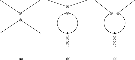
Figure 1:

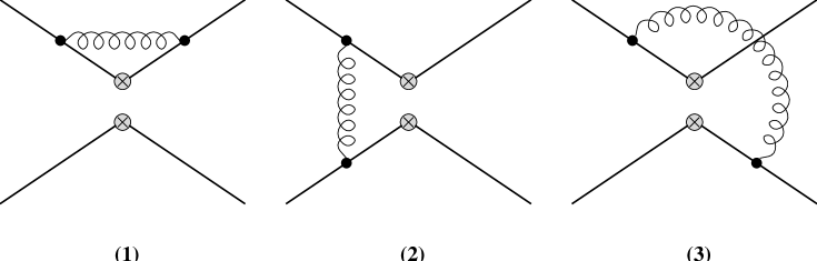
Figure 2:

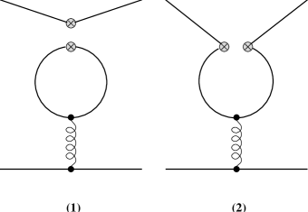
Figure 3:

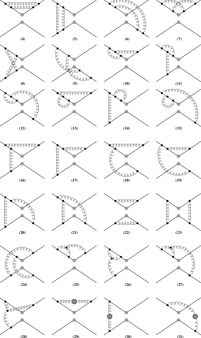
Figure 4:

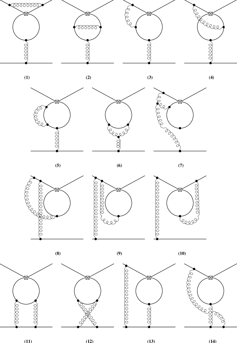
Figure 5:

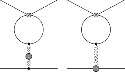
Figure 6:

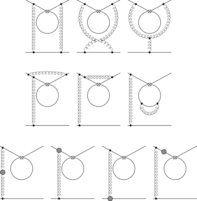
Figure 7:

Figure Captions

Figure 1:

The three basic ways of inserting a given operator into a four–point function: (a) current–current-, (b) type 1 penguin-, (c) type 2 penguin-insertion. The curled lines denote gluons. The 4-vertices “$\otimes\ \otimes$” denote standard operator insertions.

Figure 2:

One–loop current–current diagrams contributing to $\hat{\gamma}_{\rm s}^{(0)}$. The meaning of lines and vertices is the same as in fig. 1. Possible left-light or up-down reflected diagrams are not shown.

Figure 3:

One–loop type 1 and 2 penguin diagrams contributing to $\hat{\gamma}_{\rm s}^{(0)}$. The meaning of lines and vertices is the same as in fig. 1.

Figure 4:

Two–loop current–current diagrams contributing to $\hat{\gamma}_{\rm s}^{(1)}$. The meaning of lines and vertices is the same as in fig. 1. In addition shaded blobs stand for self-energy insertions. Possible left-light or up-down reflected diagrams are not shown.

Figure 5:

Two–loop penguin diagrams contributing to $\hat{\gamma}_{\rm s}^{(1)}$. The curled lines denote gluons. Square-vertices stand for type 1 and 2 penguin insertions as of figs. 1(b) and (c), respectively. Possible left-light reflected diagrams are not shown.

Figure 6:

Two–loop penguin diagrams having no $1/\varepsilon$ divergence and hence do not contribute to the anomalous dimension matrix $\hat{\gamma}_{\rm s}^{(1)}$. The meaning of lines and vertices is the same as in fig. 5. In addition shaded blobs stand for self-energy insertions or vertex corrections.

Figure 7:

Two–loop penguin diagrams vanishing identically in dimensional regularization. The meaning of lines and vertices is the same as in fig. 5. In addition shaded blobs stand for self-energy insertions or vertex corrections.

References

- [1] M. K. Gaillard and B. W. Lee, Phys. Rev. Lett. 33 (1974) 108.
- [2] G. Altarelli and L. Maiani, Phys. Lett. 52B (1974) 351.
- [3] A. I. Vainshtein, V. I. Zakharov, and M. A. Shifman, JEPT 45 (1977) 670.
- [4] F. J. Gilman and M. B. Wise, Phys. Rev. D20 (1979) 2392.
- [5] B. Guberina and R. D. Peccei, Nucl. Phys. B163 (1980) 289.
- [6] J. Bijnens and M. B. Wise, Phys. Lett. 137 B (1984) 245.
- [7] A. J. Buras and J.-M. Gérard, Phys. Lett. 192B (1987) 156.
- [8] S. R. Sharpe, Phys. Lett. 194B (1987) 551.
- [9] M. Lusignoli, Nucl. Phys. B325 (1989) 33.
- [10] J. M. Flynn and L. Randall, Phys. Lett. 224B (1989) 221, Erratum 235B (1990) 412.
- [11] G. Buchalla, A. J. Buras, and M. K. Harlander, Nucl. Phys. B337 (1990) 313.
- [12] G. Altarelli, G. Curci, G. Martinelli, and S. Petrarca, Nucl. Phys. B187 (1981) 461.
- [13] A. J. Buras and P. H. Weisz, Nucl. Phys. B333 (1990) 66.
- [14] A. J. Buras, M. Jamin, M. E. Lautenbacher, and P. H. Weisz, Nucl. Phys. B370 (1992) 69; addendum ibid. Nucl. Phys. B375 (1992) 501.
- [15] A. J. Buras, M. Jamin, and M. E. Lautenbacher, Two–Loop Anomalous Dimension Matrix for Weak Non-Leptonic Decays II: , Technical University Munich preprint, TUM-T31-30/92; Max-Planck-Institut preprint, MPI-PAE/PTh 107/92 .
- [16] A. J. Buras, M. Jamin, and M. E. Lautenbacher, Effective Hamiltonians for and Non-Leptonic Decays beyond Leading Logarithms in the Presence for Electroweak Penguins, Technical University Munich preprint, in preparation, TUM-T31-35/92 .
- [17] S. Wolfram, Mathematica – A System for Doing Mathematics by Computer., Addison - Wesley Publishing Company Inc., 1991.
- [18] M. Jamin and M. E. Lautenbacher, Technical University Munich preprint, TUM-T31-20/91 (1991), to appear in Comp. Phys. Comm. .
- [19] G. ‘t Hooft and M. Veltman, Nucl. Phys. B44 (1972) 189.
- [20] P. Breitenlohner and D. Maison, Comm. Math. Phys. 52 (1977) 11, 39, 55.
- [21] R. Tarrach, Nucl. Phys. B183 (1981) 384.
- [22] W. A. Bardeen, A. J. Buras, and J.-M. Gérard, Phys. Lett. 180B (1986) 133.
- [23] W. A. Bardeen, A. J. Buras, and J.-M. Gérard, Nucl. Phys. B293 (1987) 787.
- [24] M. J. Dugan and B. Grinstein, Phys. Lett. B256 (1991) 239.
- [25] A. Pich and E. de Rafael, Nucl. Phys. B358 (1991) 311.
- [26] H. Klugberg-Stern and J.-B. Zuber, Phys. Rev. D12 (1975) 467, 482, 3159.
- [27] S. D. Joglekar and B. W. Lee, Ann. Phys. 97 (1976) 160.
- [28] W. S. Deans and J. A. Dixon, Phys. Rev. D18 (1978) 1113.
- [29] D. Espriu, Phys. Rev. D28 (1983) 349.
- [30] L. F. Abbott, Nucl. Phys. B185 (1981) 189.
- [31] J. G. Körner, D. Kreimer, and K. Schilcher, Z. Phys. C54 (1992) 503.