Properties of Low-Lying Heavy-Light Mesons

Abstract

We present preliminary results for $f_{B}$ and masses of low-lying heavy-light mesons in the static limit. Calculations were performed in the quenched approximation using multistate smearing functions generated from a Hamiltonian for a spinless relativistic quark. The $2S$–$1S$ and $1P$–$1S$ mass splittings are measured. Using the $1P$–$1S$ charmonium splitting to set the overall scale, the ground state decay constant $f_{B}$, is $319\pm 11$(stat) MeV.

1 INTRODUCTION

Lattice gauge calculations of heavy-light meson structure are of both theoretical and phenomenological interest.[1] One immediate goal of these calculations is to obtain precise quantitative results for masses, decay constants, and form factors in the static approximation, where the heavy quark propagator is replaced by a timelike Wilson line. One difficulty which plagued early, exploratory calculations of the pseudoscalar decay constant $f_{B}$ was the problem of isolating the ground state contribution to the propagator of the local weak current. Because of the proximity of excited states and their sizeable overlap with the local current, a large separation in time was required, with an accompanying loss of statistics. Recent attempts to overcome this problem have employed nonlocal $\bar{Q}q$ operators (in a fixed gauge[2]) smeared over a cube[3] or wall source[4]. By measuring the asymptotic behavior of both the smeared-smeared ($SS$) and smeared-local ($SL$) propagators, one can reduce the systematic error associated with excited state contributions. However, it is likely that such smearing functions are too crude to obtain accurate values of the parameters of the low-lying heavy-light states.[5] This is illustrated in Table 1.

Table 1: The overlap amplitudes between various cube smearing functions and the approximate wavefunctions for the ground state $|0\rangle$ and first three excited states ($|1\rangle$, $|2\rangle$, and $|3\rangle$) for $\beta=5.9$ and $\kappa=0.158$ on a $16^{3}$ lattice.

$cube$	$|0\rangle$	$|1\rangle$	$|2\rangle$	$|3\rangle$
point	0.208	0.234	0.285	0.344
3	0.568	0.480	0.362	0.126
5	0.764	0.304	0.010	-0.220
7	0.800	-0.024	-0.296	-0.197
9	0.746	-0.330	-0.301	-0.122
11	0.663	-0.546	-0.099	-0.207
wall	0.459	-0.687	0.477	0.002

It is important, therefore, to develop new techniques which allow the extraction of the properties of heavy-light states from relatively short times. Here we report preliminary results obtained using the multistate smearing method discussed elsewhere [6, 7]. The hallmark of a pure, isolated ground state meson is an effective mass plot which is constant in time. In Figs. 1 and 2, we show our results for both the $SS$ and $SL$ local effective mass plots at $\beta=6.1,\kappa=0.151$, on a set of (48) $24^{3}\times 48$ lattices. On the horizontal axis is the time $T$ in lattice units. On the vertical axis is $\ln(C_{SS}(T{-}1)/C_{SS}(T))$.

The $SS$ local effective mass reaches its asymptotic value around $T=2$, while the $SL$ propagator is nearly asymptotic after $T=3$.

The results exhibit a single consistent plateau at $ma=0.619\pm 0.006$ over a large range of $T$ for both $SS$ and $SL$ propagators. The determination of the fitted value of the effective mass will be discussed in Section 4. We note here that the effect of the off-diagonal entries in the covariance matrix of the data for the two correlators has been included.[8]

These mass plots convincingly demonstrate the effectiveness of our smearing method in isolating the ground state.

Figure 1: $\kappa=0.151$ $SS$ effective mass plot.

Figure 2: $\kappa=0.151$ $SL$ effective mass plot.

2 WAVEFUNCTIONS

The basics of the multistate smearing method and the choice of the Hamiltonian to generate the smearing wavefunctions are reported by Thacker [7]. The agreement between the spinless relativistic quark model (SRQM) wavefunctions and the lattice QCD wavefunctions is discussed in detail there.

In the analysis presented here a two state smearing matrix was used. After a few iterations of the multistate smearing method a rough value of the mass parameter $\mu$ (in the SRQM) was determined. The output approximate ground state wavefunction at each $\kappa$ value $|0\rangle$ was extracted and used with the first excited state $|1\rangle$ generated from the SRQM. These were the two states used as smearing functions

Two points need to be made about this variation of the multistate analysis:

(1) The states are not exactly orthogonal. If $x=\langle 0|1\rangle$, then an orthonormal pair of states can be obtained by replacing $|1\rangle$ by $|1^{\prime}\rangle$ given by:

$$|1^{\prime}\rangle=(|1\rangle-x|0\rangle)/\sqrt{1-x^{2}}$$ (1)

This effect is included here but was not included in previously presented results. The effect on $f_{B}$ is approximately 12 percent.

(2) The state $|0\rangle$ varies with light quark hopping parameter $\kappa$ and this variation has some statistical fluctuation, which is reflected in the variation with $\kappa$ of our results.

3 RENORMALIZATION

In order to extract continuum results from our lattice calculation, the matrix element calculated in the lattice effective theory must be related to the corresponding quantity in the continuum. This matching is done in perturbation theory in two steps. The first step is to relate the operator (in this case the axial current) in the continuum effective theory to its counterpart in the full theory [9, 10]:

$$Z_{\rm eff}=1-\frac{g^{2}}{12\pi^{2}}(\frac{3}{2}\ln{\frac{m^{2}_{b}}{\mu^{2}}}-2).$$ (2)

We use the 1992 particle data book average [11] for $\alpha_{S}\equiv g^{2}/4\pi$ at the scale $\mu=a^{-1}$ and mass $m_{b}=5$ GeV. In the second step the lattice current is compared to the corresponding current in the continuum effective theory [9, 10]:

$$Z_{\rm lat}=1+\frac{g^{2}}{12\pi^{2}}20.37.$$ (3)

The renormalization of the axial current is then $Z_{A}^{-1}=Z_{\rm eff}Z_{\rm lat}$. Table 2 lists the renormalization constants for all the lattices analyzed here. We use the results for the 1P–1S splitting in charmonium to obtain $a^{-1}$ [12].

Table 2: The current renormalizations for different lattices

lattice	$\beta$	$Z_{\rm eff}$	$Z_{\rm lat}$	$Z_{A}$
$12^{3}\times 24$	5.7	0.90	1.33	0.83
$16^{3}\times 32$	5.9	0.96	1.31	0.79
$24^{3}\times 48$	6.1	1.00	1.30	0.77

4 ANALYSIS

We now discuss the statistical analysis leading to our results for $f_{B}$. In the first and second subsections below, we will explain the methodology leading to the central values and statistical errors quoted in our abstract and conclusions. In the third subsection, we will look at variations in the analysis procedure and their impact on these results. Variations are partly attributable to the remaining systematic errors in the computation, allowing an estimate of the magnitude of these errors.

We present results from three different lattices as listed in table 3. The gauge configurations are separated by 500 ($12^{3}\times 24,\beta=5.7$), 2000 ($16^{3}\times 32,\beta=5.9$), and 4000 ($24^{3}\times 48,\beta=6.1$) pseudo-heat-bath sweeps respectively. They were fixed to machine accuracy in Coulomb gauge using Fourier acceleration. We use the Wilson action for the light quarks. We present results from a single $\kappa$ value at $\beta=5.7$ and $\beta=6.1$. At $\beta=5.9$, the range $\kappa=0.154-0.159$ includes 0.154, 0.156, 0.157, 0.158, and 0.159.

Table 3: The lattices and parameters

lattice	$\beta$	confs.	$\kappa_{\rm light}$
$12^{3}\times 24$	5.7	48	0.165
$16^{3}\times 32$	5.9	48	0.154–0.159
$24^{3}\times 48$	6.1	48	0.151

4.1 Effective Masses and Selection of Fit Range

The effective mass plots for the $24^{3}\times 48$ lattices shown in Figs. 1 and 2 exhibit the asymptotic ground state signal starting at quite small times. However, at small times, even with carefully chosen wave functions, there are significant contributions to smeared source–smeared sink ($SS$) and smeared source–local sink ($SL$) correlators from higher energy states with the same quantum numbers as the $B$ meson. This is apparent below time $3$ in the $\beta=5.9$ $\kappa=0.158$ $SS$ effective mass plot,

Figure 3: $\kappa=0.158$ $SS$ effective mass plot.

depicted in Figure 3.

From time slice 3 on, the local effective mass is consistent with a constant function of time. This is plausible from inspection of the plot itself, which has the rms (not jackknife) errors plotted in addition to the means. To confirm this, we fit the logarithm of the $SS$ correlator to a linear function over the range of times 2–9, and found $\chi^{2}$=8.9 for 6 degrees of freedom. If the lower limit of the fit range is reduced to 1, $\chi^{2}$ increases to 12.1 for 7 degrees of freedom. These values of $\chi^{2}$ are obtained from a single fit using 48 gauge field configurations. To obtain the effective mass and its statistical error, this fit is jackknifed using 12 subensembles, each with 4 of the 48 lattices removed. Using the fit range 2–9, we find $ma$=0.664 $\pm$ 0.011 (statistical).

We now turn to the corresponding $SL$ effective mass plot,

Figure 4: $\kappa=0.158$ $SL$ effective mass plot.

depicted in Figure 4. This correlator has much smaller fluctuations (note the change in scale for the ordinate), and is capable of revealing statistically significant variations in the local effective mass over the range 2–9. Such variations are apparent in effective mass plots at lower values of $\kappa$ (not depicted), and can be ascribed to an admixture of higher energy states with the same quantum numbers as the $B$ meson. Calculations of $\chi^{2}$ for various fits at $\kappa=0.154$ suggest that the lower limit of the fit range should be increased to 5. Using the fit range 5–9, for the $\kappa$=0.158 $SL$ correlator we find that $ma=0.667$ $\pm$0.009 (jackknife).

The $\kappa=0.158$ effective masses from the two correlators appear to be consistent to within one standard deviation. However, monitoring $\chi^{2}$ for a simultaneous fit that requires the two correlators to have a common effective mass gives a more precise indication, since the statistical fluctuations of the $SS$ and $SL$ correlators may be correlated. We therefore performed fits on all $16^{3}\times 32$ data (five $\kappa$ values) using a large variety of fit intervals (demanding a common slope for the corresponding $SS$ and $SL$ correlators). We looked for fit intervals of at least three units of time which had $\chi^{2}$ per degree of freedom near one. We selected the lowest value of the lower limit of the fit range that met these conditions. For the $16^{3}\times 32$ data, the fit range so selected was 5–9. For the single $\kappa$ value at $12^{3}\times 24$, we selected 3–9, and for $24^{3}\times 48$, we selected 4–12. Intra-kappa correlations were included[8]. We will discuss the effect of variations of the fit range and inter-kappa correlations in Subsection 4.3.

4.2 Results for $f_{B}$

In Figures 3 and 4 the horizontal line superimposed on the local effective masses is the common mass obtained from a simultaneous jackknife fit to the $SS$ and $SL$ correlators using the fit interval 5–9. The $\kappa$=0.158 results are representative of the results for each of the five $\kappa$ values.

Table 4: Fitted parameters as a function of $\kappa$ at $\beta=5.9$

$\kappa$	0.159	0.158	0.157	0.156	0.154
$f_{B}$	324	316	356	344	364
	$\kern 5.00002pt11$	$\kern 5.00002pt10$	$\kern 5.00002pt11$	$\kern 5.00002pt10$	$\kern 5.00002pt10$
$ma$	0.659	0.662	0.687	0.687	0.710
	0.014	0.010	0.009	0.008	0.007
$m^{\prime}a$	0.940	0.935	0.950	0.945	0.954
	0.015	0.013	0.013	0.012	0.012

Once the common mass and two intercepts have been obtained, the value of $f_{B}$ at each $\kappa$ value is determined from the intercepts of the $SS$ and $SL$ fits. These results are presented in Table 4, which also contains the effective mass of the meson in lattice units as a function of $\kappa$. Below each quantity is its jackknife uncertainty. $m^{\prime}$ will be discussed in Section 5.

We then extrapolate $f_{B}$ to $\kappa_{c}$ the critical value of $\kappa$. We measured $\kappa_{c}=0.1597\pm 0.0001$. Since the dependence on $\kappa$ is weak, the uncertainty in $\kappa_{c}$ has a negligible (of order 1 MeV) effect on the results.

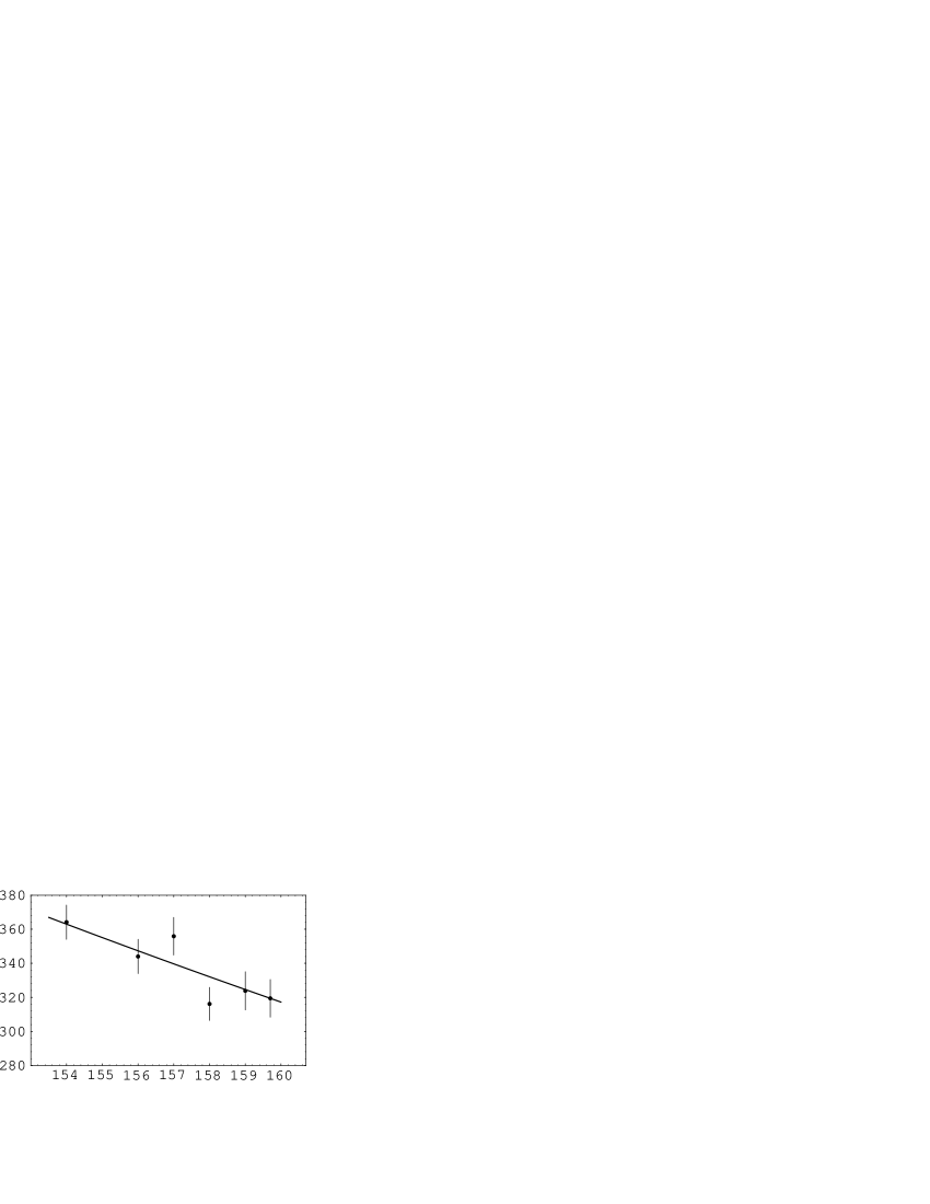
Figure 5: $f_{B}$ as a function of $\kappa$.

The results for the extrapolation as well as the results in Table 4 are plotted in Figure 5. At $\kappa_{c}$, we find for the decay constant $f_{B}=319\pm 11~{}{\rm MeV~{}(jackknife).}$ The slope with respect to $\kappa^{-1}$ is 188 $\pm$ 32 MeV. The extrapolated value of $f_{B}$ and slope with respect to $\kappa^{-1}$ are superimposed on the Monte Carlo data. The value plotted at $\kappa$=0.1597 is the extrapolated value of $f_{B}$ with its errors. The nonlinearity from using $\kappa$ as the horizontal axis rather than $\kappa^{-1}$ is imperceptible in the superimposed fit, and were we to have fit linearly in $\kappa$ rather than $\kappa^{-1}$ we would have changed the extrapolated value of $f_{B}$ and the (transformed) slope negligibly relative to the statistical errors. We note that the $\chi^{2}$ was 51 for 44 degrees of freedom.

We conclude this section by noting our results for $f_{B}$ in the static limit from $\beta=5.7$ $\kappa=0.165$ and $\beta=6.1$ $\kappa=0.151$. In the former case using the fit range 3–9, we find $f_{B}$=351 $\pm$ 13 MeV ($a^{-1}$= 1.15 GeV) and in the latter case using the fit range 4–12, we find $f_{B}$=359 $\pm$ 7 MeV ($a^{-1}$= 2.43 GeV). Using the pion mass to determine the corresponding value of $\kappa$ for $\beta=5.9$ we obtain from our fit to the $\beta=5.9$ data the corresponding values of $f_{B}$. They are $f_{B}=330$ MeV for $\beta=5.7$ and $f_{B}=367$ MeV for $\beta=6.1$.

4.3 Dependence on Analysis Procedure

In this subsection, we investigate the dependence of our results on (1) the fit interval, and (2) the inclusion of inter-kappa entries in the covariance matrix. Perhaps the most interesting of the variations in analysis is changing the admixture of the excited state. This will be discussed in the Section 5.

The dependence of $f_{B}$ on fit interval has been investigated by rerunning the analysis over the other fit ranges, in addition to the primary range 5–9. We have reproduced the analog of Figure 5 in

Figure 6: $f_{B}$ as a function of $\kappa$.

Figure 6. The results from the additional fit ranges are displaced slightly from their true $\kappa$ values. From left to right, they are 6–10, 5–9, 4–8, and 3–7. In general, the values are consistent with those of the primary fit range, 5–9, except at small values of $\kappa$ where it has already been noted that the $\chi^{2}$ per degree of freedom indicates that excited states are contributing when the lower limit of the fit range is less than 5.

We now consider the impact of inter-kappa correlations. It is apparent from comparing the $\kappa=0.158$ effective mass plots with those of other $\kappa$ values (not depicted), that there are strong correlations between corresponding quantities at different $\kappa$ values. The reason these were not included in our analysis is that with 50 data points per configuration (5 $\kappa$’s and 5 T’s for SS and SL) it is impossible to compute a nonsingular covariance matrix. To investigate the effect on the extrapolated value of $f_{B}$, we therefore reduced the number of $\kappa$ values to 2, selecting $\kappa$=0.158 and $\kappa$=0.156. We then performed the fit with and without the inter-kappa entries of the covariance matrix, and found that a decrease in the fitted and extrapolated values of $f_{B}$ resulted from including inter-kappa correlations. However these effects are in all cases less than the one sigma level. Larger statistics would allow us to study the impact of inter-kappa correlation with more $\kappa$ values in the simultaneous fit.

5 EXCITED STATES

In this section, we will examine evidence for the first radially excited state of the $B$ meson, and study the impact of the admixture of this wave function. Preliminary results for the orbitally excited states are presented in the second subsection. Finally, finite volume systematics are discussed in the last subsection.

5.1 Radial Excitations

We begin this subsection by looking at the effect on the fitted values of $f_{B}$ of the admixture of the states created by the first radially excited state smearing function. The smearing function for the analyses in the preceding section was the linear combination of smearing functions which diagonalized a two-by-two matrix of $SS$ correlators which was averaged over the same range as the primary fit range. For the $16^{3}\times 32$ data, the admixture of the trial first excited state increased from 5% to 7% with increasing $\kappa$.

To see the impact of this 5 to 7% admixture on the final

Figure 7: $f_{B}$ as a function of $\kappa$.

results, in Figure 7 we have replotted the data shown in Figure 5 along with the values of $f_{B}$ obtained from the undiagonalized smearing function. The additional data is displaced slightly from its correct $\kappa$ value for visibility. The extrapolated value of $f_{B}$ using the undiagonalized smearing function is 333 $\pm$ 12 MeV, a 4% increase.

We now examine the linear combination of the trial ground and first excited states which is orthogonal to that used for the ground state. Since we do not have correlators involving states with higher radial excitations, we expect that this orthogonal state is missing contributions from higher radial excitations of the same order as the mixing of the trial ground and first excited state. It is neverthelesss interesting

Figure 8: $\kappa=0.158$ $SS$ excited state effective mass.

to study the effective mass plots obtained from this orthogonal linear combination, which is mostly the trial first excited state. In Figure 8 we plot the $SS$ local effective mass for

Figure 9: $\kappa=0.158$ $SL$ excited state effective mass.

this correlator at $\kappa=0.158$, and in Figure 9 we plot the corresponding $SL$ correlator. The same criteria to determine the fit interval as in the ground state were used, and gave a fit interval from 3–5. The excited state effective masses in lattice units, $m^{\prime}a$, using this fit range are presented in Table 4. As usual, this is a common effective mass fitted to both the $SS$ and $SL$ correlator. The $2S$–$1S$ splitting in lattice units, $m^{\prime}a{-}ma$, decreases from 0.281 to 0.244 as $\kappa$ goes from 0.159 to 0.154.

The decay constants of the excited state for the five $\kappa$ values are approximately 600 MeV with a variation in $\kappa$ and jackknife errors both less than $\pm 15$ MeV. A slight trend is toward larger decay constants with increasing $\kappa$. The value of the decay constant, $f_{B}^{\prime}$, extrapolated to $\kappa_{c}$ is $618\pm 11$ MeV (stat). The quality of the plateau is much less convincing than for the $\beta=5.9$ ground state. The two-state approximation may induce larger systematic errors here than for the ground state. In addition, finite volume effects may be larger for the excited states. One indication supporting these preliminary results is that the values of the effective mass and decay constant are increased by about one sigma only if the fit range is changed to 4–6.

5.2 Orbital Excitations

The lowest P wave heavy-light mesons have light quark total angular momenta $j_{l}=1/2$ and $3/2$. Each of these states is degenerate with the $J=0,1$ for the $j_{l}=1/2$ state and $J=1,2$ for the $j_{l}=3/2$ state. Smearing functions for these P wave heavy-light mesons can be generated from the SRQM with the mass parameter $\mu$ which gives the best fit for the S wave ground state.

To date only a preliminary analysis has been performed on the P waves. The results for the mass splittings are given in Table 5.

Table 5: The mass splittings (in MeV) for the lowest heavy-light P states at $\beta=5.9$ for various light quark $\kappa$ values.

$\kappa$	$1P_{1/2}-1S$	$1P_{3/2}-1P_{1/2}$
0.158	$386\pm 90$	$43\pm 102$
0.156	$395\pm 86$	$59\pm 95$
0.154	$416\pm 81$	$62\pm 90$

Considerable refinement will be required before the splitting between the $j_{l}=1/2$ and $3/2$ states can be observed clearly.

5.3 Finite Volume Corrections

The systematic effects of finite volume are under study. It would be expected that these effects are more pronounced for the excited states than for the ground state because the RMS radius for excited states is larger than for the ground state. The excellent agreement between the SRQM wavefunctions and the measured wavefunctions of the $1S$, $1P$, and $2S$ heavy-light states reported by Thacker [7]. allows us to estimate the effects of finite volume with our periodic boundary conditions using SRQM results. We calculated the static energies using 48 Coulomb gauge fixed configurations at $\beta=5.9$ for lattices of spatial size $12^{3}$, $16^{3}$, and $20^{3}$. Using the mass parameter $\mu$ needed in the SRQM (obtained from our study of the heavy-light mesons on the $16^{3}\times 32$ lattices) we estimated the effects on various mass and wavefunction parameters at the other two volumes. The results are shown in Table 6.

Table 6: Finite volume effects in the SRQM. Variation of eigenvalues and properties of the eigenstates for the ground and radially excited states. Results are at $\beta=5.9$. $\epsilon_{n}$ denotes the eigenvalue for the $1S(n=0)$ and $2S(n=1)$ states.

Measure	$12^{3}$	$16^{3}$	$20^{3}$
$\epsilon_{0}$	$0.900$	$0.912$	$0.911$
$\epsilon_{1}-\epsilon_{0}$	$0.251$	$0.278$	$0.277$
$|\Psi_{0}(0)|$	$0.193$	$0.209$	$0.206$
$|\Psi_{1}(0)|$	$0.239$	$0.236$	$0.236$
$<r_{0}^{2}>^{1/2}$	$3.320$	$3.01$	$3.03$
$<r_{1}^{2}>^{1/2}$	$5.09$	$5.50$	$5.53$

The typical variation between results at $12^{3}$ and $16^{3}$ are 10% or more, while the variation between $16^{3}$ and $20^{3}$ have dropped to a few percent. The validity of these model results is presently being checked by a complete analysis of heavy-light mesons on the $12^{3}\times 24$ and $20^{3}\times 40$ lattices.

6 CONCLUSIONS

By using good approximate wave functions in a multistate smearing calculation, it is possible to control the systematic errors associated with extracting the decay constant from nonasymptotic time. Our results are very encouraging, not only for the present calculations, but for the determination of other B-meson decay parameters and form factors. All such calculations require the external meson to be in a pure eigenstate (i.e. on shell). By using the optimized smearing functions discussed here, this requirement can be met with a minimum separation between the B-meson source and the electroweak vertex, greatly improving the precision of the results.

We find that at $\beta=5.9$ and $\kappa=\kappa_{\rm critical}$

$$f_{B}=319\pm 11({\rm stat})\times{Z_{A}\over 0.79}\times\left({a^{-1}\over 1.75{\rm GeV}}\right)^{3/2}{\rm MeV}\;$$ (4)

The efficacy of our smearing method is even greater at $\beta=6.1$ as can be seen by comparing Figs. 1 and 2 with Figs. 3 and 4 with the same physical volume.

In addition to ground state properties, this method allows extraction of the properties of the lowest radially and orbitally excited states. Our results for these quantities are preliminary, and we expect more precise estimates to be obtained by further analysis.

Further numerical studies are required to check the finite volume effects, determine the effect of using an improved action for the light quarks, and include additional light quark mass values at $\beta=6.1$ which will allow a better determination of the scaling behaviour of these properties of low-lying heavy-light states.

ACKNOWLEDGEMENTS

We thank George Hockney, Andreas Kronfeld, and Paul Mackenzie for joint lattice efforts without which this analysis would not have been possible. JMF thanks the Nuffield Foundation for support under the scheme of Awards for Newly Appointed Science Lecturers. The numerical calculations were performed on the Fermilab ACPMAPS computer system developed by the CR&D department in collaboration with the theory group. This work is supported in part by the Department of Energy under Contract Nos. DE–AT03–88ER 40383 Mod A006–Task C and DE-AS05-89ER40518, and the National Science Foundation under Grant No. PHY-90-24764.

References

- [1] See E. Eichten, Nucl. Phys. B(Proc.Suppl.) 20 (1991) 475 and the references therein.
- [2] See C. Alexandrou, et al, Phys. Lett B 256 (1991) 60 for gauge invariant smearing.
- [3] C. R. Allton et al, Nucl. Phys. B376 (1992) 172.
- [4] C. Bernard, C. M. Heard, J. Labrenz, and A. Soni, Nucl. Phys. B (Proc. Suppl.) 26 (1992) 384.
- [5] S. Hashimoto and Y. Saeki, Mod. Phys. Lett. A7 (1992) 509.
- [6] A. Duncan, E. Eichten, and H. Thacker, Nucl. Phys. B(Proc.Suppl.) 26 (1992) 391; 26 (1992) 394.
- [7] A. Duncan, E. Eichten, and H. Thacker (these proceedings).
- [8] D. Toussaint, in From Actions to Answers–Proceedings of the 1989 Theoretical Advanced Study Institute in Elementary Particle Physics, T. DeGrand and D. Toussaint, eds., (World, 1990).
- [9] E. Eichten, B. Hill, Phys. Lett. B 234 (1990) 253, and Phys. Lett. B 240 (1990) 193.
- [10] Ph. Boucaud, C. L. Lin, and O. Pene, Phys. Rev. D 40 (1989) 1529, and Phys. Rev. D 41 (1990) 3541(E).
- [11] The Particle Data Group, Phys. Rev. D 45 (1992).
- [12] A. X. El-Khadra, G. M. Hockney, A. S. Kronfeld, P. B. Mackenzie, Phys. Rev. Lett. 69 (1992) 729.