^∗ Partially supported by the Swiss National Foundation

ABSTRACT

We present an effective Lagrangian parameterization describing scalar, vector, and axial-vector bound states, originating from a strong breaking of the electroweak symmetry, based on the global symmetry $SU(N)_{L}\otimes SU(N)_{R}$. In this approach vector and axial-vector bound states are gauge bosons associated to a hidden $SU(N)_{L}\otimes SU(N)_{R}$ symmetry. After the gauging of the electroweak symmetry, the corrections to the self-energies of the standard model gauge bosons are calculated and bounds on the parameter space of the model arising from precision measurements are studied. The self-energy corrections arise from spin 1 mixings, pseudogoldstones loops, pseudogoldstone-spin 1 loops, and tadpole terms. The one-loop terms tend to decrease both isospin conserving and isospin violating corrections. Careful calculation for standard $SU(8)$ QCD-scaled technicolor shows that strictly this model (which has however serious theoretical difficulties on his own) is still marginally allowed at present experimental precision.

1 Introduction

The possibility of a new strong interacting sector being at the origin of the symmetry breaking in the electroweak theory is coming to be quantitatively testable, after recent precision measurements, particularly at LEP. We shall deal here with the contributions expected from such strong sector to the vector boson self-energy corrections.

An expected feature of such strong sector is the occurence of resonances in the TeV range. The possibility of spin one resonances is particularly interesting, as they would, already through mixing effects, affect the self-energies of the standard model gauge bosons. In addition, loop effects, contributed from both spin-1 and spin-0 particles, whenever they are present, are also expected to be relatively non negligible and to bear on the comparison with experiments.

To describe the new strong sector we would like to remain as much as possible general, without assuming any particular explicit dynamical realization, for which no definite proposal has been advanced so far. To provide for such general frame we had developed a model, the BESS model, which was essentially constructed on the standpoint of custodial symmetry and gauge invariance.

The original BESS was based on the minimal chiral structure $SU(2)_{L}\times SU(2)_{R}$, but it can be easily extended to a larger $SU(N)_{L}\times SU(N)_{R}$ structure. In such a case its most apparent feature is the presence of spin-0 pseudogoldstones. Extended BESS has been specialized to standard $SU(8)$ technicolor and the conclusion was drawn that the latest experimental data would exclude conventional QCD-scaled technicolor with $N_{TC}$ technicolors and $N_{d}$ technidoublets at 90 % CL for $N_{TC}N_{d}\geq 12$ [1]. It is unnecessary to emphasize that such simple forms of technicolor have always had to face theoretical difficulties from their very beginning. This is one reason why we prefer to go on with the experimental testing of the idea of a possible strong electroweak sector within a general frame such as BESS, rather than by adopting any definite dynamical model.

The extended BESS model is based on a chiral global $SU(N)_{L}\times SU(N)_{R}$, and it contains explicit vector and axial-vector resonances (like the techni-$\rho$ of ordinary technicolor). The phenomenology of ordinary technicolor would correspond to a specialization of extended BESS.

The simplest construction for extended BESS uses a local copy of the global chiral symmetry and goes through classification of the relevant invariants. The same results follow from the hidden gauge symmetry approach. The standard electroweak $SU(2)\times U(1)$ and $SU(3)$ are gauged and a definite mixing scheme emerges for the gauge bosons and the vector and axial-vector resonances. The physical photon and the physical gluon remain massless and coupled to their conserved currents.

The quantitative estimates will be restricted to the ”historical” case $N=8$, although a number of results are more general. Through their mixings with the gauge bosons of $SU(2)_{L}\times U(1)\times SU(3)_{c}$, some of the vector and axial vector resonances acquire a coupling to quarks and leptons, and are thus expected to be produced at proton-proton and electron-positron colliders of sufficient high energy. In $SU(8)$ these spin-1 bosons are an $SU(2)$ vector triplet and axial triplet, an overall singlet, and a vector color octet, the last one susceptible to be produced through the stronger color interaction.

The effective charged current-current interaction of extended BESS reproduces the SM interaction, after identification of the relevant scale parameter with the root of the inverse Fermi coupling. Also, for any chiral $SU(N)_{L}\otimes SU(N)_{R}$, it can be seen that the neutral current-current interaction strength corresponds to a $\rho$-parameter equal to 1, because of the diagonal $SU(N)$ which is supposed to remain unbroken. All these results are of course corrected by radiative effects.

If one tries to compare $SU(8)$-BESS with the original $SU(2)$-BESS one sees that one main difference, concerning low energy effective interaction, lies in the role of the additional singlet vector-resonance, mentioned above. In addition the extension has new features, notably the appearance of pseudogoldstones.

In section 2 we present the extended BESS model. In section 3 we evaluate the tree level corrections arising from BESS to the SM gauge boson self-energies, whereas the results of the one-loop calculation are given in sections 4 and 5. Section 6 is devoted to the numerical discussion of our results, which are further enumerated in section 7. In the appendices are collected some useful formulas and results.

2 The extended BESS model

To construct the extended BESS model we proceed analogously to ref. [2], but starting now from a global symmetry $SU(N)_{L}\otimes SU(N)_{R}$, rather than $SU(2)_{L}\otimes SU(2)_{R}$. In order to do that, one introduces a local copy of the global symmetry, $[SU(N)_{L}\otimes SU(N)_{R}]_{local}$. One also enforces the idea that when the new vector and axial-vector particles decouple, one should obtain the non-linear $\sigma$-model Lagrangian, describing the Goldstone bosons, transforming as the representation $(N,N)$ of $SU(N)_{L}\otimes SU(N)_{R}$, corresponding to the breaking of $SU(N)_{L}\otimes SU(N)_{R}\to SU(N)_{L+R}$

$${\cal L}={v^{2}\over 2N}Tr\left[(\partial_{\mu}U)(\partial^{\mu}U)^{\dagger}\right]$$ (2.1)

To introduce both vector and axial-vector particles, we assume the following factorization of $U$

$$U=LM^{\dagger}R^{\dagger}$$ (2.2)

where $L,~{}M,~{}R$, transform according to the following representations of

$$G=[SU(N)_{L}\otimes SU(N)_{R}]_{global}\otimes[SU(N)_{L}\otimes SU(N)_{R}]_{local}$$

as

$$L\in({N},0,{N},0)~{}~{}~{}~{}~{}M\in(0,0,{N},{N})~{}~{}~{}~{}~{}R\in(0,{N},0,{N})$$ (2.3)

that is:

$$L^{\prime}=g_{L}Lh_{L}~{}~{}~{}~{}~{}M^{\prime}=h_{R}^{\dagger}Mh_{L}~{}~{}~{}~{}~{}R^{\prime}=g_{R}Rh_{R}$$ (2.4)

where

$$g_{L}\in({SU(N)_{L}})_{global}~{}~{}~{}~{}~{}g_{R}\in({SU(N)_{R}})_{global}$$

$$h_{L}\in({SU(N)_{L}})_{local}~{}~{}~{}~{}~{}h_{R}\in({SU(N)_{R}})_{local}$$ (2.5)

In this way we have:

$$U^{\prime}=g_{L}Ug_{R}^{\dagger}$$ (2.6)

that is,

$$U\in({N},{N},0,0)$$ (2.7)

and, therefore, $U$ does not see the local symmetry (hidden gauge symmetry). The Lagrangian (2.1) is obviously invariant under the discrete transformation $U\to U^{\dagger}$, which corresponds to (parity transformation):

$$L\to R~{}~{}~{}~{}~{}M\to M^{\dagger}~{}~{}~{}~{}~{}R\to L$$ (2.8)

Proceeding in a completely standard way, we can build up covariant derivatives with respect to the local group:

$$D_{\mu}L=\partial_{\mu}L-L{{\bf L}_{\mu}}$$

$$D_{\mu}R=\partial_{\mu}R-R{{\bf R}_{\mu}}$$

$$D_{\mu}M=\partial_{\mu}M-M{{\bf L}_{\mu}}+{{\bf R}_{\mu}}M$$ (2.9)

where ${{\bf L}_{\mu}}$ and ${{\bf R}_{\mu}}$ are the Lie algebra valued gauge fields of $({SU(N)_{L}})_{local}$ and $({SU(N)_{R}})_{local}$ respectively.

We can now construct the invariants of our original group extended by the parity operation defined in eq. (2.9). We find

$${I}_{1} = {\rm Tr}({L}^{\dagger}D_{\mu}{L}-M^{\dagger}D_{\mu}M-M^{\dagger}{R}^{\dagger}(D_{\mu}{R})M)^{2}$$ (2.10)

$${I}_{2} = {\rm Tr}({L}^{\dagger}D_{\mu}{L}+M^{\dagger}{R}^{\dagger}(D_{\mu}{R})M)^{2}$$ (2.11)

$${I}_{3} = {\rm Tr}({L}^{\dagger}D_{\mu}{L}-M^{\dagger}{R}^{\dagger}(D_{\mu}{R})M)^{2}$$ (2.12)

$${I}_{4} = {\rm Tr}(M^{\dagger}D_{\mu}M)^{2}$$ (2.13)

Using these invariants we can write the most general Lagrangian with at most two derivatives in the form:

$${\cal L}=-\frac{v^{2}}{16}(a{I}_{1}+b{I}_{2}+c{I}_{3}+d{I}_{4})+~{}kinetic~{}terms~{}for~{}the~{}gauge~{}fields$$ (2.14)

where $a,~{}b,~{}c,~{}d$ are free parameters and furthermore the gauge coupling constant for the fields ${{\bf L}_{\mu}}$ and ${{\bf R}_{\mu}}$ is the same.

It is not difficult to see that this Lagrangian is the same one would obtain from the hidden gauge symmetry approach [3]. The requirement of getting back the non-linear $\sigma$-model in the limit in which the gauge fields ${{\bf L}_{\mu}}$ and ${{\bf R}_{\mu}}$ are decoupled is satisfied by imposing the following relation among the parameters $a,b,c,d$

$$a+\frac{cd}{c+d}=1$$ (2.15)

We can now gauge the previous effective Lagrangian with respect to the standard gauge group $SU(3)_{c}\otimes SU(2)_{L}\otimes U(1)_{R}$ by the following substitutions:

$$D_{\mu}{L} \to D_{\mu}{L}=\partial_{\mu}{L}-{L}(V_{\mu}-A_{\mu})+{\bf A}_{\mu}{L}$$ (2.16)

$$D_{\mu}{R} \to D_{\mu}{R}=\partial_{\mu}{R}-{R}(V_{\mu}+A_{\mu})+{\bf B}_{\mu}{R}$$ (2.17)

$$D_{\mu}M \to D_{\mu}{M}=\partial_{\mu}M-M(V_{\mu}-A_{\mu})+(V_{\mu}+A_{\mu})M$$ (2.18)

where $V_{\mu}=({{\bf R}_{\mu}}+{{\bf L}_{\mu}})/2$ and $A_{\mu}=({{\bf R}_{\mu}}-{{\bf L}_{\mu}})/2$ are the fields describing the new vector and axial-vector resonances, whereas ${\bf A}_{\mu}$ and ${\bf B}_{\mu}$ are linear combinations of the gauge fields of the standard gauge group (see later for a more precise definition).

The $SU(N)$ generators satisfy the algebra

$$[T^{A},T^{B}]=if^{ABC}T^{C}$$ (2.19)

and are normalized by ${\rm Tr}(T^{A}T^{B})=\frac{1}{2}\delta^{AB}$.

The $V$ and $A$ bosons can be decoupled by sending $g^{\prime\prime}\to\infty$. In this limit, the mass of the $W$ bosons is the SM mass with $v\simeq 246~{}GeV$.

The effective Lagrangian (2.15) describes the interactions among the SM gauge bosons, the new vector and axial-vector resonances and the Goldstone bosons.

We will work in the unitary gauge both for the standard gauge fields, defined by $\pi^{a}=0$, and for the $V$ and $A$ bosons given by the following choice:

$${L} = {R}^{\dagger}=\exp\left({\frac{2i\pi^{A}T^{A}}{v}}{\frac{d}{c+d}}\right)$$ (2.20)

$$M = \exp\left(-{\frac{4i\pi^{A}T^{A}}{v}}{\frac{c}{c+d}}\right)$$ (2.21)

To avoid cumbersome notations we we shall restrict in the following to $N=8$, to which the quantitative discussion will be limited, except for some occasional more general remarks.

We will denote the $SU(8)$ gauge fields as $V^{A}=(V^{a},{\tilde{V}}^{a},V_{D},V_{8}^{\alpha},V_{8}^{a\alpha},V_{3}^{\mu i},{\bar{V}}_{3}^{\mu i})$, where $\mu=(0,a)$ ($a$ being an $SU(2)$ index), and $i=1,2,3$ is a color index. An analogous notation will be used for $A^{A}$ and the Goldstone bosons $\pi^{A}$. The $SU(8)$ generators are shown for convenience in Appendix A. In the following we will make use of the notations:

$${\bf A}_{\mu} = 2igW^{a}_{\mu}T^{a}+i\sqrt{2}g_{s}G^{\alpha}_{\mu}T^{\alpha}_{8}+2iyg^{\prime}Y_{\mu}T_{D}$$ (2.22)

$${\bf B}_{\mu} = 2ig^{\prime}Y_{\mu}(T^{3}+yT_{D})+i\sqrt{2}g_{s}G^{\alpha}_{\mu}T^{\alpha}_{8}$$ (2.23)

$$V_{\mu} = ig^{\prime\prime}V_{\mu}^{A}T^{A}$$ (2.24)

$$A_{\mu} = ig^{\prime\prime}A_{\mu}^{A}T^{A}$$ (2.25)

with $A,B=1,\ldots,63$; $a,b=1,2,3$; $\alpha,\beta=1,\ldots,8$ and $y=1/\sqrt{3}$ (for future convenience, we have not substitute its numerical value). We have denoted by $W,~{}Y,~{}G$ the standard model (SM) gauge bosons and by $g,~{}g^{\prime},g_{s}$ their coupling constants, while $g^{\prime\prime}$ is the self coupling of the $V$ and $A$ bosons. Let us consider the quadratic terms in eq. (2.15) to see which is the structure of the mixing between the SM gauge bosons and the new vector and axial-vector resonances:

$${\cal L}^{(2)} = \frac{v^{2}}{8}\Big{[}a(gW^{a}-g^{\prime}\delta^{a3}Y)^{2}+b(gW^{a}+g^{\prime}\delta^{a3}Y-g^{\prime\prime}V^{a})^{2}+b(2yg^{\prime}Y-g^{\prime\prime}V_{D})^{2}$$ (2.26)

$$+b(\sqrt{2}g_{s}G^{\alpha}-g^{\prime\prime}V^{\alpha}_{8})^{2}+bg^{\prime\prime 2}\sum_{A\neq a,D,\alpha}(V^{A})^{2}+c(gW^{a}-g^{\prime}\delta^{a3}Y+g^{\prime\prime}A^{a})^{2}$$

$$+cg^{\prime\prime 2}\sum_{A\neq a}(A^{A})^{2}+dg^{\prime\prime 2}(A^{A})^{2}\Big{]}+~{}kinetic~{}terms$$

In the charged sector the mixing terms are the same as in ref. [2].

In the neutral sector the mixing involves the fields $W^{3},~{}Y,~{}V^{3},~{}V_{D},~{}A^{3}$. The mixing with $V_{D}$, which makes the gauge boson sector of the $SU(8)$-BESS different in a non trivial way from the model based on $SU(2)_{L}\otimes SU(2)_{R}$, is parametrized by $y$.

The mass eigenvalues in the limit $g^{\prime\prime}\rightarrow\infty$ are (see Appendix B):

$$M_{\gamma}^{2} = 0$$ (2.27)

$$M_{W}^{2} \simeq \frac{v^{2}}{4}g^{2}\left(1-(\frac{g}{g^{\prime\prime}})^{2}\left(\frac{1}{1-r_{V}}-\frac{z^{2}}{1-r_{A}}\right)\right)$$ (2.28)

$$M_{Z}^{2} \simeq \frac{v^{2}}{4}G^{2}\left(1-(\frac{g}{g^{\prime\prime}})^{2}\left(\frac{1}{c^{2}_{\theta}-r_{V}}(c^{2}_{2\theta}+4y^{2}s_{\theta}^{4})+\frac{z^{2}}{c^{2}_{\theta}-r_{A}}\right)\right)$$ (2.29)

$$M_{V}^{2} \simeq \frac{v^{2}}{4}\frac{g^{2}}{r_{V}}$$ (2.30)

$$M_{A}^{2} \simeq \frac{v^{2}}{4}\frac{g^{2}}{r_{A}}$$ (2.31)

where $G=\sqrt{g^{2}+g^{\prime 2}}$, $s_{\theta}=\sin\theta=g^{\prime}/G$, $x=g/g^{\prime\prime}$, and

$$r_{V}=\frac{x^{2}}{b}~{}~{}~{}~{}~{}r_{A}=\frac{x^{2}}{c+d}~{}~{}~{}~{}~{}z=\frac{c}{c+d}$$ (2.32)

Notice that, in the limit considered, all vector and all axial-vector masses are degenerate.

Finally we observe that the mixing angle for the colored sector in the large $g^{\prime\prime}$ limit is $\simeq-\sqrt{2}g_{s}/g^{\prime\prime}$. The linear combinations corresponding to the gluons remain massless whereas the orthogonal ones are degenerate in mass with all the other $V$ bosons (in the large $g^{\prime\prime}$ limit).

For simplicity we do not add a direct coupling of the $V$ and $A$ bosons to the fermions. Therefore only the gauge bosons $V^{a},~{}V_{D},~{}V_{8}^{\alpha},~{}A^{a}$ can be produced via quark-antiquark, through their mixing with the SM gauge bosons.

For what concerns the low energy interactions, in the charged sector things go exactly as in the $SU(2)$-BESS model [2], and the charged current-current interaction coincides with the SM one by the identification $\sqrt{2}G_{F}=1/v^{2}$.

The neutral current-current interaction strength is given by:

$$\frac{4}{\sqrt{2}}\rho~{}G_{F}=\frac{2}{v^{2}}({\bar{\cal M}}^{-1})_{11}$$ (2.33)

with ${\bar{\cal M}}$ given in Appendix B. Also in this case (as in ref. [2]) we get $({\bar{\cal M}}^{-1})_{11}=1$ and therefore $\rho=1$. This is due to the global unbroken diagonal $SU(8)$. The same is true in general for $SU(N)\otimes SU(N)$. Finally, from the neutral current, one can extract the expression for the electric charge

$$e=g^{\prime}c_{\theta}c_{\psi}c_{\eta}$$ (2.34)

with the angles $\psi$ and $\eta$ defined in Appendix B. The difference with respect to the $SU(2)$-BESS is contained in the mixing angle $\eta$ (which vanishes for $y=0$) corresponding to the $V_{D}$ contribution.

3 Gauge boson self-energies

We will now compute the corrections to the self-energies of the SM gauge bosons from the new vector and axial-vector resonances and from the pseudogoldstones. We will consider first the tree-level contribution induced by the mixing of the $V$ and $A$ bosons with the $W$, $Z$ and $\gamma$.

We define the scalar part of the vector boson self-energies through the relation:

$$\Pi_{ij}^{\mu\nu}(q^{2})=-i\Pi_{ij}(q^{2})g^{\mu\nu}+q^{\mu}q^{\nu}~{}terms$$ (3.1)

where the indices $i$ and $j$ run over the ordinary gauge vector bosons. The self-energy corrections are obtained by separating out the SM terms from the bilinear part of the Lagrangian, given in eq. (2.27), and by computing, with the remaining terms, all the tree-level self-energy graphs which are one-particle-irreducible with respect to the lines $W$, $\gamma$ and $Z$. This is equivalent to solve the equations of motion for the fields $V^{\pm}$, $A^{\pm}$, $V^{3}$, $V_{D}$ and $A^{3}$ by using again the quadratic Lagrangian.

Since the mixing in the charged sector of $SU(8)$-BESS is the same as in $SU(2)$-BESS, we get the same result for the $WW$ self-energy correction as in ref. [4]:

$$\Pi_{WW}(q^{2})=-x^{2}\left(M^{2}_{V}\frac{q^{2}}{q^{2}-M^{2}_{V}}+z^{2}M^{2}_{A}\frac{q^{2}}{q^{2}-M^{2}_{A}}\right)$$ (3.2)

In the neutral sector we choose to work with the SM combinations:

$$W^{3}=c_{\theta}~{}Z+s_{\theta}~{}\gamma$$ (3.3)

$$Y=-s_{\theta}~{}Z+c_{\theta}~{}\gamma$$ (3.4)

The solutions of the equations of motion for the new bosons are:

$$V^{3} = x\frac{M^{2}_{V}}{M^{2}_{V}-q^{2}}(W^{3}+\tan\theta~{}Y)$$ (3.5)

$$V_{D} = 2xy\tan\theta\frac{M^{2}_{V}}{M^{2}_{V}-q^{2}}Y$$ (3.6)

$$A^{3} = -xz\frac{M^{2}_{A}}{M^{2}_{A}-q^{2}}(W^{3}-\tan\theta~{}Y)$$ (3.7)

By substituting these relations in the equations of motion for the $W^{3}$ and $Y$ fields we can read the expression for the self-energy corrections $\Pi_{33}$, $\Pi_{30}$ and $\Pi_{00}$ as

$$\Pi_{33}(q^{2}) = \Pi_{WW}(q^{2})$$ (3.8)

$$\Pi_{30}(q^{2}) = -\frac{s_{\theta}}{c_{\theta}}{\bar{M}}^{2}_{W}x^{2}\left(\frac{1}{r_{V}}\frac{q^{2}}{q^{2}-M^{2}_{V}}-\frac{z^{2}}{r_{A}}\frac{q^{2}}{q^{2}-M^{2}_{A}}\right)$$ (3.9)

$$\Pi_{00}(q^{2}) = -\frac{s^{2}_{\theta}}{c^{2}_{\theta}}{\bar{M}}^{2}_{W}x^{2}\left((1+4y^{2})\frac{1}{r_{V}}\frac{q^{2}}{q^{2}-M^{2}_{V}}+\frac{z^{2}}{r_{A}}\frac{q^{2}}{q^{2}-M^{2}_{A}}\right)$$ (3.10)

where ${\bar{M}}^{2}_{W}=(v^{2}g^{2})/4$.

It is convenient to introduce the following combinations (see ref. [5]):

$$\epsilon_{1} = \frac{\Pi_{33}(0)-\Pi_{WW}(0)}{M^{2}_{W}}$$ (3.11)

$$\epsilon_{2} = \frac{\Pi_{WW}(M^{2}_{W})-\Pi_{WW}(0)}{M^{2}_{W}}-\frac{\Pi_{33}(M^{2}_{Z})-\Pi_{33}(0)}{M^{2}_{Z}}$$ (3.12)

$$\epsilon_{3} = \frac{c_{\theta}}{s_{\theta}}\frac{\Pi_{30}(M^{2}_{Z})-\Pi_{30}(0)}{M^{2}_{Z}}$$ (3.13)

The new $V_{D}$ boson does not affect the $\epsilon_{i}$ parameters because it contributes only to $\Pi_{00}$. Therefore we recover the same expressions as for $SU(2)$-BESS, or

$$\epsilon_{1}=0~{}~{}~{}~{}\epsilon_{2}\simeq 0,~{}~{}~{}~{}\epsilon_{3}\simeq x^{2}(1-z^{2})$$ (3.14)

where the last two results are obtained for large $M_{V,A}$ ($M_{V,A}>>M_{W,Z}$).

The additional contribution to $\Pi_{00}$ affects the electric charge and the $Z$ mass definition, as can be seen by eqs. (2.35) and (2.30).

The reason we get the same result as in ref. [4] is that the new $V_{D}$ boson mixes only with $Y$ (see eq. (2.27)). This means that our result can be extended to a $SU(N)_{L}\otimes SU(N)_{R}$ model. This is due to the fact that in these models the new fields associated to the diagonal generators will be mixed only with the hypercharge field $Y$.

It is interesting to notice that the same result for $\epsilon_{3}$ can be obtained by using the dispersive representation which had been already given in refs. [6] [7]. In fact, by using the relation $\epsilon_{3}=(\alpha_{em}/4s^{2}_{\theta})S$ we get:

$$\epsilon_{3}=-\frac{g^{2}}{4\pi}\int_{0}^{\infty}\frac{ds}{s^{2}}\left[{\rm Im}~{}\Pi_{VV}(s)-{\rm Im}~{}\Pi_{AA}(s)\right]$$ (3.15)

where $\Pi_{VV(AA)}$ is the correlator of the vector (axial-vector) currents. If we assume vector meson dominance, we can saturate the eq. (3.15) with the $V$ and $A$ resonances:

$${\rm Im}~{}\Pi_{VV(AA)}(s)=-\pi g^{2}_{V(A)}\delta(s-M^{2}_{V(A)})$$ (3.16)

where $g_{V}$ and $g_{A}$ are the couplings of the vector and axial-vector currents to the $V$ and $A$ fields respectively. These couplings can be obtained directly from eq. (2.15), using eqs. (2.31-32):

$$g_{V}=-2\frac{M^{2}_{V}}{g^{\prime\prime}}~{}~{}~{}~{}~{}~{}~{}~{}g_{A}=2z\frac{M^{2}_{A}}{g^{\prime\prime}}$$ (3.17)

and substituting eqs. (3.16-17) in eq. (3.15) we get the tree-level contribution to $\epsilon_{3}$ given in eq. (3.14).

We will now consider the one-loop contributions to the self-energies in order to calculate the corrections to the $\epsilon_{i}$.

There are four kinds of loops. The first is a loop of Goldstones, the second is a loop of one Goldstone boson and one $V$ boson, the third one is a loop of one Goldstone boson and one $A$ boson and the fourth is a tadpole of Goldstones. Also, since we will work with the fields appearing in the Lagrangian of eq. (2.15) which are not the mass eigenstates, we will take into account all the possible mixings on the external legs.

For the calculation of the loop contributions to $\epsilon_{i}$ it is useful to compute from the effective Lagrangian given in eq. (2.15) (in the unitary gauge given by eqs. (2.25-26) and with $\pi^{a}=0$) trilinear and quadrilinear terms in the colorless sector.

The trilinear terms in the gauge boson neutral sector are ($y=1/\sqrt{3}$) :

$$i{\cal L}_{neutr}^{(3)} = \Big{\{}\Big{[}g_{W\pi\pi}(W^{3}_{\mu}+\tan\theta~{}Y_{\mu})+g_{V\pi\pi}V^{3}_{\mu}\Big{]}(-{\tilde{\pi}}^{-}\partial^{\mu}{\tilde{\pi}}^{+}-\pi_{8}^{\alpha-}\partial^{\mu}\pi_{8}^{\alpha+}$$

$$+{\bar{P}}_{3}^{-i}\partial^{\mu}P_{3}^{-i}-{\bar{P}}_{3}^{+i}\partial^{\mu}P_{3}^{+i})+(-\frac{4}{3}g_{W\pi\pi}\tan\theta~{}Y_{\mu}-\frac{2}{\sqrt{3}}g_{V\pi\pi}V_{D\mu})$$

$$({\bar{P}}_{3}^{0i}\partial^{\mu}P_{3}^{0i}+{\bar{P}}_{3}^{3i}\partial^{\mu}{P}_{3}^{3i}+{\bar{P}}_{3}^{-i}\partial^{\mu}P_{3}^{-i}+{\bar{P}}_{3}^{+i}\partial^{\mu}P_{3}^{+i})$$

$$+\Big{[}g_{WV\pi}(W^{3}-\tan\theta~{}Y)-g_{VA\pi}A^{3}\Big{]}({\tilde{V}}^{+}{\tilde{\pi}}^{-}+V_{8}^{\alpha+}\pi_{8}^{\alpha-}-{\bar{P}}_{3}^{-i}{\cal V}_{3}^{-i}+{\bar{P}}_{3}^{+i}{\cal V}_{3}^{+i})$$

$$+\Big{[}-g_{WA\pi}(W^{3}+\tan\theta~{}Y)+g_{VA\pi}V^{3}\Big{]}({\tilde{A}}^{+}{\tilde{\pi}}^{-}+A_{8}^{\alpha+}\pi_{8}^{\alpha-}-{\bar{P}}_{3}^{-i}{\cal A}_{3}^{-i}+{\bar{P}}_{3}^{+i}{\cal A}_{3}^{+i})$$

$$+\Big{[}-\frac{4}{3}g_{WA\pi}\tan\theta~{}Y+\frac{2}{\sqrt{3}}g_{VA\pi}V_{D}\Big{]}({\bar{P}}_{3}^{0i}{\cal A}_{3}^{0i}+{\bar{P}}_{3}^{3i}{\cal A}_{3}^{3i}+{\bar{P}}_{3}^{-i}{\cal A}_{3}^{-i}+{\bar{P}}_{3}^{+i}{\cal A}_{3}^{+i})$$

$$-h.c.\Big{\}}$$

The notation used here for the fields is given in Appendix C, in particular ${\cal V}_{3}^{\mu i}$ and ${\cal A}_{3}^{\mu i}$ are defined analogously as $P_{3}^{\mu i}$ and

$$g_{W\pi\pi}=\frac{g}{2}\left[1-\frac{1}{2}\frac{x^{2}}{r_{V}}(1-z^{2})\right]~{}~{}~{}~{}g_{V\pi\pi}=\frac{g^{\prime\prime}}{4}\frac{x^{2}}{r_{V}}\left(1-z^{2}\right)$$ (3.19)

$$g_{WV\pi}=\frac{v}{4}gg^{\prime\prime}\frac{x^{2}}{r_{V}}(1-z^{2}\frac{r_{V}}{r_{A}})~{}~{}~{}g_{VA\pi}=\frac{v}{4}zg^{\prime\prime 2}\frac{x^{2}}{r_{V}}\left(\frac{r_{V}}{r_{A}}-1\right)~{}~{}~{}g_{WA\pi}=x~{}g_{VA\pi}$$ (3.20)

We have also used the relations

$$a=1-\frac{x^{2}}{r_{A}}(1-z)z~{}~{}~{}~{}~{}~{}b=\frac{x^{2}}{r_{V}}~{}~{}~{}~{}~{}~{}c=z\frac{x^{2}}{r_{A}}~{}~{}~{}~{}~{}~{}d=\frac{x^{2}}{r_{A}}(1-z)$$ (3.21)

obtained from eqs. (2.16) and (2.33). Notice that we have not written down the trilinear terms coming from the kinetic terms.

The relevant quadrilinear couplings turn out to be those involving two colorless gauge fields and two Goldstone bosons. Furthermore, only the terms containing the $V^{3}$, $V^{\pm}$, $V_{D}$, $A^{3}$, $A^{\pm}$ fields contribute to the calculation of the correction to the $W,Y$ self-energies. In fact, only these components of $V^{A}$ and $A^{A}$ mix with the standard gauge bosons. We list here the terms which are relevant for the computation of $\epsilon_{i}$:

$${\cal L}^{(4)} = \Big{\{}\Big{[}g_{VV\pi\pi}(V_{3}^{2}-A_{3}^{2})+W_{3}(g_{WV\pi\pi}V_{3}-g_{WA\pi\pi}A_{3})\Big{]}$$ (3.22)

$$\times({\tilde{\pi}}^{-}{\tilde{\pi}}^{+}+\pi_{8}^{\alpha-}\pi_{8}^{\alpha+}+{\bar{P}}_{3}^{+i}P_{3}^{+i}+{\bar{P}}_{3}^{-i}P_{3}^{-i})$$

$$+\Big{[}g_{VV\pi\pi}(V^{+}V^{-}-A^{+}A^{-})+W^{+}(g_{WV\pi\pi}V^{-}-g_{WA\pi\pi}A^{-})\Big{]}$$

$$\times({\tilde{\pi}}^{-}{\tilde{\pi}}^{+}+({\tilde{\pi}}^{3})^{2}+\pi_{8}^{\alpha-}\pi_{8}^{\alpha+}+(\pi_{8}^{\alpha 3})^{2}$$

$$+{\bar{P}}_{3}^{+i}P_{3}^{+i}+{\bar{P}}_{3}^{-i}P_{3}^{-i}+2{\bar{P}}_{3}^{3i}P_{3}^{3i})+h.c.\Big{\}}$$

where

$$g_{VV\pi\pi}=\frac{g^{\prime\prime 2}}{8}z^{2}\frac{x^{2}}{r_{V}}\left(\frac{r_{V}}{r_{A}}-1\right)$$ (3.23)

$$g_{WV\pi\pi}=\frac{gg^{\prime\prime}}{8}\frac{x^{2}}{r_{V}}\left(1+z^{2}-2z^{2}\frac{r_{V}}{r_{A}}\right)$$ (3.24)

$$g_{WA\pi\pi}=\frac{gg^{\prime\prime}}{8}z\frac{x^{2}}{r_{V}}\left((1+z^{2})\frac{r_{V}}{r_{A}}-2\right)$$ (3.25)

Notice that we have not written down the quadrilinears coming from the kinetic terms. Actually, as we will see, they do not contribute to the calculation of $\epsilon_{i}$.

We have calculated the loop integrals by using a cut-off $\Lambda$, keeping also the finite terms, assuming a non vanishing mass for the Goldstone bosons and in the limit $M^{2}_{V,A}>>q^{2}$.

4 One-loop contribution to $\epsilon_{3}$

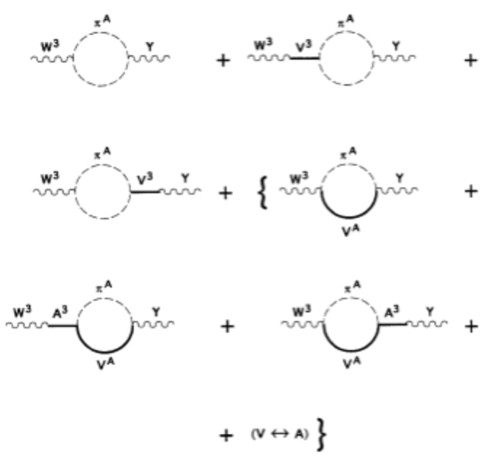
Figure 1: Graphs included in the calculation of $\epsilon_{3}^{loop}$ of eq. (4.1).

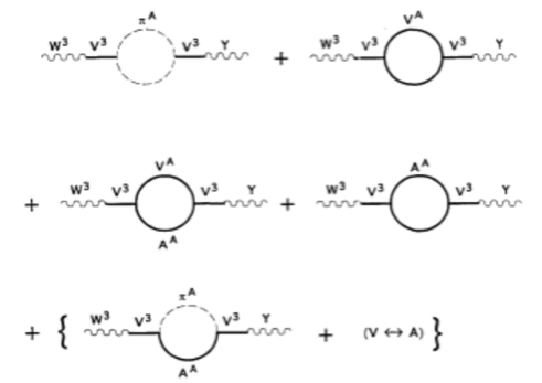
Figure 2: Corrections to $\epsilon_{3}^{loop}$ coming from the $V^{3}$ and $A^{3}$ self-energy contributions.

In Figs. 1-2 we show the graphs contributing to $\epsilon_{3}$ at one-loop level.

We have separately drawn in Fig. 2 the diagrams depending on the $V$ and $A$ self-energies. In order to correctly evaluate their contributions to $\epsilon_{3}$ one has to properly renormalize the BESS model at one-loop and then extract the finite terms coming from these graphs which are not absorbed in the redefinition of the BESS parameters. In the present calculation of $\epsilon_{3}$ we have not used this procedure but we have simply tried to estimate the dominant contribution of the $V$ and $A$ self-energy graphs by using a dispersive representation for $\epsilon_{3}$. The calculation is given in Appendix D and further comments will be given in Sect. 6.

We have not listed the tadpole loops of pseudo-Goldstone bosons (PGB) and of vector and axial-vector bosons. In fact, due to the form of the $\epsilon_{3}$ given in eq. (3.13), the seagulls do not contribute because they are independent of $q^{2}$ in the $M^{2}_{V,A}>>q^{2}$ limit.

We give here the result for the one-loop contribution obtained by summing up the graphs of Fig. 1. We have regularized the integrals with a cut-off $\Lambda$ and we have considered a non-vanishing mass $m_{\Pi}$ for the PGB’s. In fact, since $\epsilon_{3}$ is an isospin symmetric observable, we can consider the same mass for all the PGB’s. Here is the result:

$$\epsilon_{3}^{loop} \simeq \frac{g^{2}}{16\pi^{2}}\frac{5}{8}\Big{\{}\left(\log\frac{\Lambda^{2}}{m_{\Pi}^{2}}-\gamma\right)\Big{[}2-\frac{1}{2}\frac{x^{4}}{r_{V}^{2}}(1-z^{2})^{2}$$ (4.1)

$$-\frac{x^{2}}{r_{V}}(1-z^{2}\frac{r_{V}}{r_{A}})\Big{(}1-z^{2}-z^{2}(1-\frac{r_{V}}{r_{A}})\Big{)}-z^{2}\frac{x^{2}}{r_{A}}(1-\frac{r_{A}}{r_{V}})^{2}\Big{]}$$

$$-\frac{x^{2}}{r_{V}}(1-z^{2}\frac{r_{V}}{r_{A}})\Big{(}1-z^{2}-z^{2}(1-\frac{r_{V}}{r_{A}})\Big{)}\Big{(}A(m_{\Pi}^{2},M_{V}^{2})+1\Big{)}$$

$$-z^{2}\frac{x^{2}}{r_{A}}(1-\frac{r_{A}}{r_{V}})^{2}\Big{(}A(m_{\Pi}^{2},M_{A}^{2})+1\Big{)}\Big{\}}$$

where $\gamma$ is the Euler’s constant $(\simeq 0.577)$, and

$$A(m_{\Pi}^{2},M^{2}) = \frac{M^{6}+9M^{4}m_{\Pi}^{2}}{(M^{2}-m_{\Pi}^{2})^{3}}\log{\frac{m_{\Pi}^{2}}{M^{2}}}$$ (4.2)

$$+\frac{1}{6(M^{2}-m_{\Pi}^{2})^{3}}(m_{\Pi}^{6}-27m_{\Pi}^{4}M^{2}-9m_{\Pi}^{2}M^{4}+35M^{6})$$

Notice that, by decoupling the vector and axial-vector resonances (that is by taking $x=0$ in eq. (4.1)), one recovers the $SU(8)$ technicolor result (see for instance ref. [8]). The same result is obtained in the completely degenerate case: $z=1$ and $r_{V}=r_{A}$. In fact the vector and the axial-vector contributions cancel and only the PGB loops remain. Also, for $z=0$ the axial-vector resonances decouple.

5 Effects of the isospin violating terms: one-loop contribution to $\epsilon_{1}$

For the calculation of $\epsilon_{1}^{loop}$ one needs $\Pi_{33}$ and $\Pi_{WW}$ at the one-loop level.

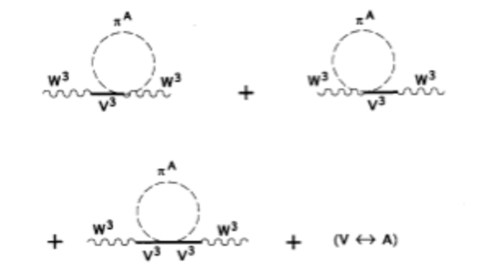
Figure 3: Tadpole graphs contributing to $\Pi_{33}$ which are relevant for the calculation of $\epsilon_{1}^{loop}$.

The graphs contributing to $\Pi_{33}$ are those given in Figs. 1-2 with the substitution ($Y\to W^{3}$) on the external leg, plus the tadpole graphs of Fig. 3. Also, as can be seen from the Lagrangian terms in eqs. (3.18) and (3.23), the graphs contributing to $\Pi_{WW}$ and to $\Pi_{33}$ are of the same kind. So, if one assumes mass degeneration for the $SU(2)$ multiplets of the pseudo-Goldstone bosons, it is easy to show that one gets again

$$\Pi_{WW}^{loop}=\Pi_{33}^{loop}$$ (5.1)

and so $\epsilon_{1}^{loop}=0$.

In the case in which the PGB masses are not $SU(2)$ symmetric one expects non vanishing contributions to $\epsilon_{1}^{loop}$ coming from the splitting.

An important property of the $SU(2)$ triplets and of the associated singlets of PGB’s is the validity of sum rules for their masses following from the symmetry structure of the theory. For a generic quadruplet $P^{+},P^{-},P^{0},P^{3}$ we can show that [9]

$$m_{P^{+}}^{2}+m_{P^{-}}^{2}=m_{P^{0}}^{2}+m_{P^{3}}^{2}$$ (5.2)

In fact in the chiral limit one has a $G=SU(2)_{L}\otimes SU(2)_{R}$ symmetry for each fermionic doublet. Then the mass matrix must be a combination of a scalar and of generators of $G\sim O(4)$ which commutes with the electric charge. Therefore the general structure of the mass matrix is

$$M^{2}=A+BK_{3}+CT_{3}$$ (5.3)

with $T_{3}=(1/2)(T_{3L}+T_{3R})$ and $K_{3}=(1/2)(T_{3L}-T_{3R})$. Notice that the $({1\over 2},{1\over 2})$ representation of $G$ to which the Goldstone bosons belong, decomposes as ${\underline{1}}+{\underline{3}}$ with respect to $O(3)\subset O(4)$ and therefore the following sum rules for the masses are implied for all the quadruplets:

$$\sum m^{2}_{\Pi}(T_{3}=0)=\sum m^{2}_{\Pi}(K_{3}=0)$$ (5.4)

which is equivalent to eq. (5.2) (see also [10]).

An important consequence of the validity of the previous sum rules is that the dependence on the cut-off $\Lambda$ (introduced to regularize the one-loop integrals) cancels and we get an ultraviolet finite result (see also [10]). Adding all the contributions from the different loops we get (for a single quadruplet):

$$\epsilon_{1}^{loop} \simeq \frac{g^{2}}{256\pi^{2}}\frac{m_{P^{+}}^{2}}{{\bar{M}}^{2}_{W}}\Big{(}-\delta_{0}^{+}\log\frac{m_{P^{+}}^{2}}{m_{P^{-}}^{2}}+F(P^{+},P^{0})+F(P^{+},P^{3})$$ (5.5)

$$+\frac{x^{2}}{r_{V}}(1-z^{2})^{2}\Big{[}\delta_{0}^{+}\log\frac{m_{P^{+}}^{2}}{m_{P^{-}}^{2}}+(1+\delta_{0}^{+})\log(1+\delta_{0}^{+})$$

$$+(1+\delta_{3}^{+})\log(1+\delta_{3}^{+})+2~{}g(\eta^{+})-(1+\delta_{3}^{+})~{}g(\eta^{3})$$

$$-(1+\delta_{0}^{+})~{}g(\eta^{0})\Big{]}\Big{)}+\Big{(}P^{+}\longleftrightarrow P^{-}\Big{)}$$

where

$$F(P^{+},P^{0})=1-\frac{(1+\delta_{0}^{+})^{2}}{\delta_{0}^{+}}\log(1+\delta_{0}^{+})$$ (5.6)

and

$$g(\eta)=\frac{1}{1-\eta}(1-\frac{\eta}{4})\log\eta~{}~{}~{}~{}~{}~{}\eta=\frac{m^{2}_{P}}{M^{2}_{V}}$$ (5.7)

with

$$\delta_{0}^{+}=\frac{m_{P^{0}}^{2}-m_{P^{+}}^{2}}{m_{P^{+}}^{2}}~{}~{}~{}~{}~{}~{}~{}\delta_{3}^{+}=\frac{m_{P^{3}}^{2}-m_{P^{+}}^{2}}{m_{P^{+}}^{2}}$$ (5.8)

and $\delta_{0}^{-}$ and $\delta_{3}^{-}$ analogously defined. The total result is obtained by collecting the similar contributions from all the quadruplets and taking into account the appropriate multiplicity in the color sector:

$$\epsilon_{1}=\epsilon_{1}(col.~{}singl.)+8\epsilon_{1}(col.~{}oct.)+3\epsilon_{1}(col.~{}tripl.)+3\epsilon_{1}(col.~{}antitripl.)$$ (5.9)

Notice that the one-loop result does not depend on the mass of the axial-vector resonances. This is due to cancellation among the terms coming from the loops of $A$ bosons and PGB’s. The presence of the axial-vectors is signalled only by the $z$ parameter entering into the quadrilinear couplings (see eqs. (3.24-25)). For $z=1$, again, the new gauge boson contributions cancel and we get the result from the PGB loops.

We have also calculated the one-loop contribution to $\epsilon_{2}$. As it is clear by comparing the definitions in eq. (3.12), we have that, within the BESS model, $\epsilon_{2}$ is depressed with respect to $\epsilon_{1}$ by a factor $\sim~{}M^{2}_{W}/M^{2}_{V}$. Therefore the further restrictions coming from the numerical analysis based on $\epsilon_{2}$ are quite irrelevant and we will not consider them.

In ref. [9] we have developed a framework for a quantitative evaluation of the PGB masses, including, besides the gauge contribution [11], also the contribution from those interactions which are responsible for the masses of the ordinary fermions. In this way, all those states which, neglecting such Yukawa terms, would remain massless, tend to acquire mass terms which are close to those of the heaviest fermions of the theory. In such a scheme a splitting among the PGB masses is unavoidable since it is due to the mass difference between the top and the bottom quarks. Furthermore in this case, mixings between the neutral components of the $SU(2)$ triplets and the associated singlets appear.

6 Numerical results

We now give a quantitative estimate of the parameters $\epsilon_{3}$ and $\epsilon_{1}$ as predicted by the BESS model. The BESS parameters are $M_{V}$, $M_{A}$, $g^{\prime\prime}$ and $z$ and one must also add to them the values of the pseudo-Goldstone masses and the cut-off $\Lambda$. To reduce the BESS parameter space we will assume the validity of the Weinberg Sum Rules (WSR), which have been shown to hold in asymptotically free gauge theories [12]:

$$\frac{1}{\pi}\int_{0}^{\infty}\frac{ds}{s}\left[{\rm Im}~{}\Pi_{VV}(s)-{\rm Im}~{}\Pi_{AA}(s)\right]=v^{2}$$

$$\frac{1}{\pi}\int_{0}^{\infty}ds\left[{\rm Im}~{}\Pi_{VV}(s)-{\rm Im}~{}\Pi_{AA}(s)\right]=0$$ (6.1)

where $\Pi_{VV(AA)}$ is the correlator of the vector (axial-vector) currents.

If we also assume vector meson dominance, we can saturate the eqs. (6.1) with the $V$ and $A$ resonances by using the relation (3.16). In this way we get

$$M^{2}_{A}=\frac{M^{2}_{V}}{z}~{}~{}~{}~{}~{}~{}~{}~{}g^{\prime\prime}=2\frac{M_{V}}{v}\sqrt{1-z}$$ (6.2)

with $0<z<1$.

With a further specialization of the BESS parameters, one can reproduce a standard technicolor scheme [1]. In the case of a $SU(N_{TC})$ scaled up version of QCD, one has:

$$M^{2}_{\rho TC} = M^{2}_{0}\frac{3}{N_{TC}}\frac{4}{N_{d}}$$

$$M^{2}_{A_{1}TC} = 2M^{2}_{\rho TC}$$ (6.3)

where $N_{d}$ is the number of technidoublets (in the present calculation $N_{d}=4$) and $M_{0}$ is a scale parameter of the order of $1~{}TeV$. By comparing with the eq. (6.2) one gets

$$z=\frac{1}{2}~{}~{}~{}~{}~{}~{}~{}~{}\frac{g}{g^{\prime\prime}}=\frac{{\bar{M}}_{W}}{M_{0}}\sqrt{\frac{N_{TC}N_{d}}{6}}$$ (6.4)

Our strategy will be to work in the context of validity of the WSR’s leaving $M_{V}$ and $z$ as free parameters. Therefore we remain with a two-dimensional parameter space plus the cut-off and the PGB masses.

Before comparing the prediction of this model for the observables $\epsilon_{i}$, we must consider the radiative corrections coming from the standard model contributions.

The BESS model has no elementary scalars and it is not a renormalizable theory. Radiative corrections for BESS can be defined only if one considers this model as a cut-off theory. We will assume the same one-loop radiative corrections as in the SM by interpreting the Higgs mass $m_{H}$ as the cut-off $\Lambda$ used to regularize the theory. In particular, in our numerical estimations, we have used the SM radiative corrections to the $\epsilon_{i}$ as given in the last of ref. [5].

The experimental limits on the $\epsilon_{i}$ come from the measured values of some weak interaction observables. The minimal set is given by $M_{W}/M_{Z},~{}A_{FB}^{l},~{}\Gamma_{l}$. One can also include the $A^{\tau}_{pol.},~{}A_{FB}^{b}$ and the low energy data, in particular neutrino-nucleus deep inelastic scattering and parity violation in Cs atoms. In the following analysis we will use the values obtained considering this larger set [13]:

$$\epsilon_{1}=(0.16\pm 0.32)10^{-2}~{}~{}~{}~{}\epsilon_{2}=(-0.72\pm 0.79)10^{-2}~{}~{}~{}~{}\epsilon_{3}=(0.00\pm 0.43)10^{-2}$$ (6.5)

Let us first consider the bounds on the BESS parameters coming from the estimation of the corrections to $\epsilon_{3}$.

In the following numerical analysis we will neglect the contribution coming from the graphs of Fig. 2. The reason is that the estimate we have given in Appendix D is reliable only when $M_{V}$ and $M_{A}$ are above threshold for the decay in $\pi\pi$ and in $\pi V$ respectively. This implies that the representations given in eqs. (D.1) and (D.4) cannot be valid for generic values of $m_{\Pi}$ and $z$. However we can make the following comments. It has already been noticed [7] that, if the PGB masses are large, $\delta\epsilon_{3}^{V}$ can be negative and decreases the tree level contribution by a sizeable amount. For instance, taking $M_{V}=1200~{}GeV$, $z=0.5$, and $m_{\Pi}=300~{}GeV$, one finds $\delta\epsilon_{3}^{V}=-0.002$, to be compared to $(\epsilon_{3}^{V})_{tree}=0.009$. In this example the conclusion holds true even by including the axial-vector contribution. One has $\delta\epsilon_{3}=-0.001$ and $(\epsilon_{3})_{tree}=0.0067$. More generally, by studying numerically $\delta\epsilon_{3}$ in eqs. (D.1)-(D.7), one sees that, for fixed $M_{V}$ and $z$, there is a window for $m_{\Pi}$, usually requiring $m_{\Pi}$ to be sufficiently large, where $\delta\epsilon_{3}$ is negative. In the cases we have analyzed, the tree-level result might be lowered by about 15%. Positive contributions to $\epsilon_{3}$ could also arise for small PGB masses $m_{\Pi}$.

Starting from eq. (4.1) and substituting the relations (6.2) which follow from the WSR’s, we obtain an expression for $\epsilon_{3}^{loop}$ which depends on the cut-off $\Lambda$, the mass of the PBG’s $m_{\Pi}$ (which we assume degenerate), the mass of the $V$ bosons and the parameter $z$. Actually the dependence on $\Lambda$ and on $M_{V}$ is very weak (in the range of values of interest that is $\sim 1-2~{}TeV$) and also the dependence on $m_{\Pi}$ is not too strong.

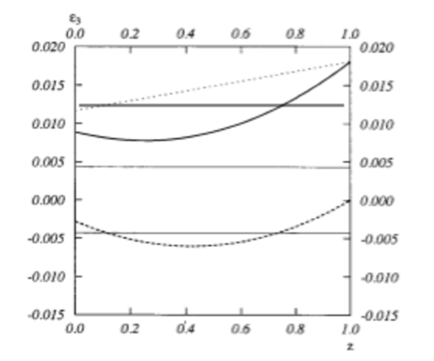
Figure 4: $\epsilon_{3}$ versus $z$ for $\Lambda=1.5~{}TeV$, $M_{V}=1~{}TeV$ and $m_{\Pi}/\Lambda=0.35$. The dotted line is the tree-level BESS model contribution plus the SM radiative corrections, the dashed line is the one-loop contribution, and the solid line is the total correction. Also shown is the experimental 1$\sigma$ band.

In Fig. 4 we plot the one-loop contribution (dashed line) to $\epsilon_{3}$ as a function of $z$ for $\Lambda=1.5~{}TeV$, $M_{V}=1~{}TeV$ and $m_{\Pi}/\Lambda=0.35$. Also reported in Fig. 4 is the tree-level contribution as given in eq. (3.14) with the substitution (6.2) summed with the SM radiative corrections (dotted line). Finally the total correction to $\epsilon_{3}$ at one-loop level is given by the solid line. By comparing this result with the experimental data given in eq. (6.5) we see how the one-loop contribution, which turns out to be negative, leads to a better agreement (in the figure the experimental $1\sigma$ band is shown).

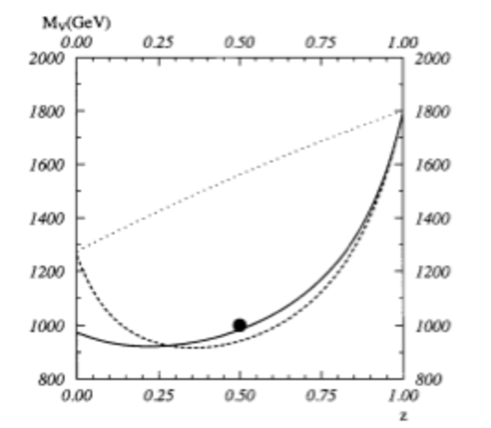
Figure 5: 90% C.L. allowed region in the plane $(z,M_{V})$ from $\epsilon_{3}$ for $\Lambda=1.5~{}TeV$. The dotted line is the lower bound on $M_{V}$ coming from the tree-level BESS model contribution plus the SM radiative corrections, the solid (dashed) line is the bound coming from the total one-loop effect for $m_{\Pi}/\Lambda=0.35$ ($m_{\Pi}/\Lambda=0.10$). The black dot shows the case of technicolor with one family of technifermions and $N_{TC}=3$.

This can be seen also in Fig. 5 where the lower bound on $M_{V}$ as a function of $z$ coming from the measure of $\epsilon_{3}$ is plotted. Again the dotted line is the lower bound coming from the tree-level plus the SM radiative corrections. The inclusion of the one-loop contribution enlarge the allowed region (the region is at 90$\%$ C.L.). In the figure it is shown how the bound varies for different values of $m_{\Pi}/\Lambda$, ranging from 0.10 (dashed line) to 0.35 (solid line). We see that the dependence is very weak. Here $\Lambda=1.5~{}TeV$. Also shown is the case of a standard technicolor theory with one family of technifermions (black dot in the figure) which is now marginally included in the 90$\%$ C.L. region. In fact the positive contribution of the PGB loops is overcompensated by the negative one coming from the loops containing the vector and the axial-vector resonances. Notice that the region shown in Fig. 5 corresponds to a pessimistic estimate in view of the previous comment on the $V-A$ self-energy contributions.

It is not difficult to see that each $SU(2)$ doublet of Pseudo Goldstone bosons, vector and axial-vector resonances gives a negative contribution to $\epsilon_{3}$. Therefore, in a model $SU(N)_{L}\otimes SU(N)_{R}$ the value of $\epsilon_{3}$ decreases by increasing $N$.

Let us quantitatively analyze the corrections to $\epsilon_{1}$ coming from isospin violating terms. In order to do this, one has to specialize the spectrum of the masses of the PGB’s.

As stressed in Section 5, the PGB mass spectrum must satisfy the sum rules (5.2). A possible simplified parameterization which is consistent with the sum rules and the discussion made in ref. [9] is the following:

$$m^{2}({\tilde{\pi}}^{\pm})=\Delta m^{2}$$ (6.6)

$$m^{2}\left(\frac{{\tilde{\pi}}^{3}-\pi_{D}}{\sqrt{2}}\right)\simeq 0$$ (6.7)

$$m^{2}\left(\frac{{\tilde{\pi}}^{3}+\pi_{D}}{\sqrt{2}}\right)=2\Delta m^{2}$$ (6.8)

$$m^{2}\left(P_{3}^{\pm i}\right)=\frac{\Lambda^{2}g_{s}^{2}}{2\pi^{2}}+\Delta m^{2}$$ (6.9)

$$m^{2}\left(\frac{P^{0i}_{3}-P_{3}^{3i}}{\sqrt{2}}\right)=\frac{\Lambda^{2}g_{s}^{2}}{2\pi^{2}}$$ (6.10)

$$m^{2}\left(\frac{P^{0i}_{3}+P_{3}^{3i}}{\sqrt{2}}\right)=\frac{\Lambda^{2}g_{s}^{2}}{2\pi^{2}}+2\Delta m^{2}$$ (6.11)

where we have used the notation given in Appendix C. In this example, the masses of the colorless sector depend only on $\Delta m$. In eq. (6.7), for numerical purposes, we have assumed a zero mass because in ref. [9] we have found that there exists an upper bound of 9 $GeV$ for $\Lambda=1~{}TeV$ (an analogous estimate comes also from other mechanisms of mass generation, see for instance ref. [14]).

The colored states get mass also from QCD corrections [11]. We have not included the octet states because for them the splitting is negligible (they receive the strongest QCD correction) and so they do not significatively contribute to $\epsilon_{1}$. For the color triplets we have assumed the same splitting $\Delta m$ as for the colorless sector while the QCD contribution is given in terms of $g_{s}$, which is the $SU(3)$ gauge coupling constant (we will use $\alpha_{s}=0.12$), and in terms of $\Lambda$ which is the ultraviolet cut-off introduced to regularize the quadratic divergence in the one-loop effective potential [11] [9] (we will take $\Lambda=1~{}TeV$).

If one follows ref. [9] $\Delta m$ is proportional to $\Lambda$ and it depends on the masses of the heaviest fermions of the theory, the top and the bottom quark. Here we will leave it as a free parameter.

The mass splitting gives rise to a mixing between the neutral component of an isotriplet and the corresponding isosinglet. This mixing does not affect the calculation of $\Pi_{33}$ and $\Pi_{30}$ since in the corresponding graphs only charged particle loops appear. On the contrary, for the calculation of $\Pi_{WW}$ one has to consider the neutral mass eigenstates in the loops.

We have calculated the corrections to $\epsilon_{1}^{loop}$ coming from the isospin violating PGB spectrum given in eq. (6.6-11), by using the expression (5.5) in the context of validity of the WSR’s.

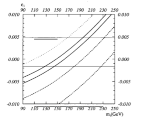
Figure 6: $\epsilon_{1}$ versus $m_{t}$ for $\Lambda=1~{}TeV$ and $M_{V}=1~{}TeV$. The dotted line corresponds to the SM radiative corrections. The band delimited by two solid (dashed) lines corresponds to $\Delta m=200~{}GeV$ ($\Delta m=300~{}GeV$) and displays the complete range of variability in $z$ ($0\leq z\leq 1$). Also shown is the experimental 1$\sigma$ band.

In Fig. 6 we show the SM radiative corrections for $\epsilon_{1}$ as a function of $m_{t}$ (dotted line). They are compared with the BESS predictions at one-loop, which include the SM radiative corrections. The band delimited by two solid (dashed) lines corresponds to $\Delta m=200(300)~{}GeV$, and displays the complete range of variability in $z$. In both cases the lower edge of the bands corresponds to $z=1$ while the upper one is for $z\sim 0.3$. The figure is done for $M_{V}=1000$ GeV. As $M_{V}$ grows the bands shrink, keeping the lower edge fixed because, in this case, only the PGB’s contribute.

We see that the one-loop contribution is negative and, as discussed for $\epsilon_{3}$, this is a general feature valid for any $SU(N)_{L}\otimes SU(N)_{R}$ ($N>2$). In fact, as it appears from equation (5.9) the total one-loop contribution arises from the sum of the quadruplets contained in the adjoint representation of $SU(8)$, and each of this contribution is negative definite. Therefore, also in this case, by increasing $N$ the value of $\epsilon_{1}$ is decreased.

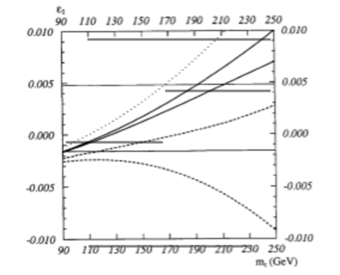
Figure 7: $\epsilon_{1}$ versus $m_{t}$ for $\Lambda=1~{}TeV$ and $M_{V}=1~{}TeV$. The dotted line corresponds to the SM radiative corrections. The band delimited by two solid (dashed) lines corresponds to $\Delta m=m_{t}$ ($\Delta m=1.5~{}m_{t}$) and displays the complete range of variability in $z$ ($0\leq z\leq 1$). Also shown is the experimental 1$\sigma$ band.

Fig. 7 is analogous to Fig. 6, but in this case, in the spirit of ref. [9], we take $\Delta m$ as a linear function of $m_{t}$. The region delimited by solid lines corresponds to $\Delta m=m_{t}$ and the one delimited by dashed lines to $\Delta m=1.5~{}m_{t}$.

In both figures the horizontal band corresponds to the $1\sigma$ experimental limit, as given in eq. (6.5). We note that the effect of the BESS correction is to weaken the upper bound on the top mass.

7 Conclusions

The main purpose of the work was the calculation of the corrections to the self-energies of the gauge bosons of the standard model from the vector and axial resonances and from the spin zero (pseudogoldstones) particles of extended BESS. The corrections affect the scalar gauge boson self-energy terms $\Pi_{WW}$, $\Pi_{33}$, $\Pi_{00}$, and $\Pi_{30}$ in the usual $SU(2)_{L}\times U(1)$ notation. For convenience, to compare with the previous BESS results, we have chosen the normalization in terms of the parameters ${\epsilon}_{1}$, ${\epsilon}_{2}$, ${\epsilon}_{3}$, but any other parametrization would be equivalent.

The mixings among vector and axial resonances and standard gauge bosons already provide for a correction calculable at the tree-level, which turns out to be the same as for $SU(2)$-BESS, that is essentially vanishing ${\epsilon}_{1}$ and ${\epsilon}_{2}$, and an ${\epsilon}_{3}$ as in $SU(2)$-BESS. This holds for any $SU(N)_{L}\times SU(N)_{R}$, the reason being that the new diagonal vector resonances only mix with the electroweak $U(1)$ gauge boson.

In addition to the self-energy corrections arising from the mixing, one has loop contributions. At one loop, one has loops of Goldstones, loops of a Goldstone and a vector resonance, or a Goldstone and an axial resonance, and finally one has to add a Goldstone tadpole graph. The model provides for the needed trilinear and quadrilinear couplings involving spin 1 and spin 0 particles. And, of course, one has also to take into account the possibilities of mixings of the external $W^{3}$ and $Y$ legs with the vector and axial-vector resonances.

For the calculation of the one-loop contributions to ${\epsilon}_{3}$, which is isospin symmetric, one can insert a common non-vanishing mass for all the pseudogoldstones. The result one finds for ${\epsilon}_{3}$ goes back to that of standard technicolor when the vector and axial-vector resonances are decoupled. One again obtains this result when the vector and axial resonances are taken as completely degenerate, due to their reciprocal cancellation in each case.

The one-loop contributions to ${\epsilon}_{1}$ vanish for degenerate masses of the $SU(2)$ pseudogoldstones multiplets, so that one has to take into account the expected multiplet splittings. Fortunately the symmetry structure of the theory implies sum rules for pseudogoldstones masses. A consequence of the sum rules is also the cancellation of possible cut-off dependent terms. The total ${\epsilon}_{1}$ is then obtained by summing on all quadruplets $P^{\pm}$, $P^{o}$, $P^{3}$ of pseudogoldstones taking their color multiplicity into account. The result at one-loop is independent of the mass of the axial-vector resonances due to cancellation between loops of pseudogoldstones and loops of axial-vectors.

Finally, concerning ${\epsilon}_{2}$, one notices that in BESS there will be a depression factor of the order $(M_{W}/M_{V})^{2}$ with respect to ${\epsilon}_{1}$ so that its role in the analysis is unimportant.

Our quantitative analysis of ${\epsilon}_{3}$ and ${\epsilon}_{1}$ has to include certain pseudogoldstone masses. For this we have used a calculation we had developed of such masses, which includes the usual gauge contributions and in addition the contributions from the interactions providing for ordinary fermion masses, in the form of effective Yukawa couplings. The would-be massless goldstones in absence of the yukawians, then acquire masses close to the heaviest fermion, with consequent mass splittings reflecting the large splitting between top and bottom quark.

As far as the BESS parameters are concerned, we have reduced them by assuming the validity of the Weinberg sum rules for the imaginary parts of the vector and axial self-energies and saturating them with vector and axial-vector dominance.

The standard, QCD scaled technicolor, would correspond to an additional specialization of the parameters contained in our set.

The numerical analysis has of course to include electroweak radiative corrections. Our assumption, physically plausible in the presence of new degrees of freedom related to a larger scale, has been to take the usual one loop radiative corrections of the standard model, by interpreting the Higgs mass occurring there as the cut-off which regularizes BESS at high momenta.

There exist experimental limits on the ${\epsilon}$’s from a set of observables including $M_{W}/M_{Z}$, $A^{\ell}_{FB}$, and $\Gamma_{\ell}$, $A^{\tau}_{pol}$, $A^{b}_{FB}$ and low energy weak data, which we have used to derive bounds on the BESS parameters.

We have illustrated in Fig. 4 the comparison with the present experimental bounds on ${\epsilon}_{3}$ (the region inside the two horizontal lines is the 1$\sigma$ band). The theoretical ${\epsilon}_{3}$ versus the BESS parameter $z$ (which weights the axial vector to vector coupling) is the solid line (the other parameters are indicated in the caption, but their role is rather insensitive). One sees that a definitive exclusion of this SU(8)-BESS is strictly yet not possible. The one loop corrections have added a negative contribution bringing closer to the experimental band. Indeed each SU(2) doublet of pseudogoldstones, vectors, and axial vectors adds a negative contribution, so that by increasing $N$ in the chiral structure $SU(N)_{R}\otimes SU(N)_{L}$ ${\epsilon}_{3}$ will further decrease.

The comparison in terms of allowed region for the BESS parameters $M_{V}$ and $z$ (in Fig. 5) from the ${\epsilon}_{3}$ experimental limitations shows the region above the solid line as the allowed one. The standard, QCD scaled, $SU(8)$ technicolor corresponds to the black dot. Inclusion of the one-loop corrections has made this theory (which is however already afflicted by other serious diseases of his own) marginally compatible, at least at present, with data.

Also, in considering the strength of the conclusions for $SU(8)$-BESS, we recall that in particular the validity of the second Weinberg sum rule has been added within the assumptions, to limit the BESS parameters.

The analysis for ${\epsilon}_{1}$ rests heavily on the isospin splittings within the pseudogoldstones multiplets. We have employed a consistent parametrization for them, supported by the theoretical analysis of their mass spectrum. The horizontal band in Fig. 6 is the experimental 1$\sigma$ band for ${\epsilon}_{1}$. Depending on the top mass, the two theoretical bounds (solid lines and dashed lines), corresponding to two different choices for the parameter characterizing the pseudogoldstones mass splittings, have consistent overlaps with the experimental band. By increasing $N$, in $SU(N)_{R}\otimes SU(N)_{L}$ more quadruplets of pseudogoldstones arise, each giving a negative contribution to ${\epsilon}_{1}$ at one loop, and the theoretical bands are increasingly lowered with respect to the SM dotted-line in Fig. 6. Similar conclusions, qualitatively, follows by explicitly exploiting the expected dependence of the splitting parameter from the top mass, with the theoretical bounds taking a different shape in this case. A common trend from these analyses of ${\epsilon}_{1}$ is that the upper bounds, implied by ${\epsilon}_{1}$ on the top mass within the standard model, get weakened in the presence of the strong electroweak sector.

The careful calculations performed in this work in terms of extended BESS continue with the program of transposing precise new experimental data into bounds for a possible strong electroweak sector, in a rather general formulation which tries to avoid reference to a particular new strong dynamics. The fact that standard QCD-scaled $SU(8)$ technicolor now appears to be marginally allowed by data, after a careful evaluation of the one loop effects, should not be interpreted as a possible revival for this model, which, as well known, has always had deep theoretical difficulties. We consider that only by keeping within a formulation as much as possible general, stressing symmetry aspects and the main expected dynamical features, one can systematically follow the increase in precision of the experimental data to circumscribe the theoretical freedom still left for some type of new electroweak strong sector.

Appendix A

The generators of the $SU(8)$ algebra are

$$T^{A}=(T^{a},{\tilde{T}}^{a},T_{D},T_{8}^{\alpha},T_{8}^{a\alpha},T_{3}^{\mu i},{\bar{T}}_{3}^{\mu i})$$ (A.1)

with $A=1,\ldots,63$, $a=1,2,3$, $\alpha=1,\ldots,8$, $\mu=(0,a)$ and $i=1,2,3$. They are normalized by

$${\rm Tr}(T^{A}T^{B})=\frac{1}{2}\delta^{AB}$$ (A.2)

We use the following representation

$$T^{a}=\frac{1}{4}\left(\begin{tabular}[]{c|c}\\ $\tau^{a}\otimes{\bf 1}_{3}$&0\\ \\ \hline\cr\\ 0&$\tau^{a}$\\ \\ \end{tabular}\right)~{}~{}~{}~{}~{}{\tilde{T}}^{a}=\frac{\sqrt{3}}{4}\left(\begin{tabular}[]{c|c}\\ $\tau^{a}\otimes{\bf 1}_{3}/3$&0\\ \\ \hline\cr\\ 0&$-\tau^{a}$\\ \\ \end{tabular}\right)$$ (A.3)

$$T_{D}=\frac{\sqrt{3}}{4}\left(\begin{tabular}[]{c|c}\\ ${\bf 1}_{2}\otimes{\bf 1}_{3}/3$&0\\ \\ \hline\cr\\ 0&$-{\bf 1}_{2}$\\ \\ \end{tabular}\right)$$ (A.4)

$$T_{8}^{\alpha}=\frac{1}{\sqrt{8}}\left(\begin{tabular}[]{c|c}\\ ${\bf 1}_{2}\otimes\lambda^{\alpha}$&0\\ \\ \hline\cr\\ 0&0\\ \\ \end{tabular}\right)~{}~{}~{}~{}~{}T_{8}^{a\alpha}=\frac{1}{\sqrt{8}}\left(\begin{tabular}[]{c|c}\\ $\tau^{a}\otimes\lambda^{\alpha}$&0\\ \\ \hline\cr\\ 0&0\\ \\ \end{tabular}\right)$$ (A.5)

$$T_{3}^{\mu i}=\frac{1}{\sqrt{8}}\left(\begin{tabular}[]{c|c}\\ 0&$\sigma_{\mu}\otimes\xi^{i}$\\ \\ \hline\cr\\ $\sigma_{\mu}\otimes\xi^{iT}$&0\\ \\ \end{tabular}\right)~{}~{}~{}~{}~{}{\bar{T}}_{3}^{\mu i}=\frac{1}{\sqrt{8}}\left(\begin{tabular}[]{c|c}\\ 0&$i\sigma_{\mu}\otimes\xi^{i}$\\ \\ \hline\cr\\ $-i\sigma_{\mu}\otimes\xi^{iT}$&0\\ \\ \end{tabular}\right)$$ (A.6)

where $\tau^{a}$ are the $SU(2)$ generators normalized by ${\rm Tr}(\tau^{a}\tau^{b})=2\delta^{ab}$, $\lambda^{\alpha}$ are the $SU(3)$ generators normalized by ${\rm Tr}(\lambda^{\alpha}\lambda^{\beta})=2\delta^{\alpha\beta}$, $\sigma^{\mu}\equiv({\bf 1}_{2},\tau^{a})$ and the $\xi^{i}$ are the three orthogonal unit vectors in the three-dimensional vector space.

The commutation rules

$$[T^{A},T^{B}]=if^{ABC}T^{C}$$ (A.7)

are obtained by using

$$\left[\tau^{a},\tau^{b}\right]=2i\epsilon^{abc}\tau^{c}$$ (A.8)

$$\left[\lambda^{\alpha},\lambda^{\beta}\right]=2if^{\alpha\beta\gamma}\lambda^{\gamma}$$ (A.9)

$$\left[\lambda^{\alpha},\lambda^{\beta}\right]_{+}=\frac{4}{3}\delta^{\alpha\beta}+2d^{\alpha\beta\gamma}\lambda^{\gamma}$$ (A.10)

We get the following non vanishing commutators:

$$\left[T^{a},T^{b}\right] = \frac{i}{2}\epsilon^{abc}T^{c}$$ (A.11)

$$\left[T^{a},{\tilde{T}}^{b}\right] = \frac{i}{2}\epsilon^{abc}{\tilde{T}}^{c}$$ (A.12)

$$\left[T^{a},T_{8}^{b\alpha}\right] = \frac{i}{2}\epsilon^{abc}T_{8}^{c\alpha}$$ (A.13)

$$\left[T^{a},T_{3}^{\mu i}\right] = \frac{i}{2}\delta^{\mu b}\epsilon^{abc}T_{3}^{ci}$$ (A.14)

$$\left[T^{a},{\bar{T}}_{3}^{\mu i}\right] = \frac{i}{2}\delta^{\mu b}\epsilon^{abc}{\bar{T}}_{3}^{ci}$$ (A.15)

$$\left[{\tilde{T}}^{a},{\tilde{T}}^{b}\right] = \frac{i}{2}\epsilon^{abc}(T^{c}-\frac{2}{\sqrt{3}}{\tilde{T}}^{c})$$ (A.16)

$$\left[{\tilde{T}}^{a},T_{8}^{b\alpha}\right] = \frac{i}{2\sqrt{3}}\epsilon^{abc}T_{8}^{c\alpha}$$ (A.17)

$$\left[{\tilde{T}}^{a},T_{3}^{\mu i}\right] = -\delta^{\mu 0}\frac{i}{\sqrt{3}}{\bar{T}}_{3}^{ai}-\delta^{\mu a}\frac{i}{\sqrt{3}}{\bar{T}}_{3}^{0i}-\delta^{\mu b}\frac{i}{2\sqrt{3}}\epsilon^{abc}T_{3}^{ci}$$ (A.18)

$$\left[{\tilde{T}}^{a},{\bar{T}}_{3}^{\mu i}\right] = \delta^{\mu 0}\frac{i}{\sqrt{3}}T_{3}^{ai}+\delta^{\mu a}\frac{i}{\sqrt{3}}T_{3}^{0i}-\delta^{\mu b}\frac{i}{2\sqrt{3}}\epsilon^{abc}{\bar{T}}_{3}^{ci}$$ (A.19)

$$\left[T_{D},T_{3}^{\mu i}\right] = -\frac{i}{\sqrt{3}}{\bar{T}}_{3}^{\mu i}$$ (A.20)

$$\left[T_{D},{\bar{T}}_{3}^{\mu i}\right] = \frac{i}{\sqrt{3}}T_{3}^{\mu i}$$ (A.21)

$$\left[T_{8}^{\alpha},T_{8}^{\beta}\right] = \frac{i}{\sqrt{2}}f^{\alpha\beta\gamma}T_{8}^{\gamma}$$ (A.22)

$$\left[T_{8}^{\alpha},T_{8}^{a\beta}\right] = \frac{i}{\sqrt{2}}f^{\alpha\beta\gamma}T_{8}^{a\gamma}$$ (A.23)

$$\left[T_{8}^{\alpha},T_{3}^{\mu i}\right] = -\frac{1}{4\sqrt{2}}\left[[(\lambda^{\alpha})_{im}-(\lambda^{\alpha})_{mi}]T_{3}^{\mu m}+i[(\lambda^{\alpha})_{im}+(\lambda^{\alpha})_{mi}]{\bar{T}}_{3}^{\mu m}\right]$$ (A.24)

$$\left[T_{8}^{\alpha},{\bar{T}}_{3}^{\mu i}\right] = -\frac{1}{4\sqrt{2}}\left[[(\lambda^{\alpha})_{im}-(\lambda^{\alpha})_{mi}]{\bar{T}}_{3}^{\mu m}-i[(\lambda^{\alpha})_{im}+(\lambda^{\alpha})_{mi}]T_{3}^{\mu m}\right]$$ (A.25)

$$\left[T_{8}^{a\alpha},T_{8}^{b\beta}\right] = \frac{i}{2}\delta^{\alpha\beta}\epsilon^{abc}\left[T^{c}+\frac{1}{\sqrt{3}}{\tilde{T}}^{c}\right]+\frac{i}{\sqrt{2}}\left[\delta^{ab}f^{\alpha\beta\gamma}T_{8}^{\gamma}+\epsilon^{abc}d^{\alpha\beta\gamma}T_{8}^{c\gamma}\right]$$ (A.26)

$$\left[T_{8}^{a\alpha},T_{3}^{\mu i}\right] = -\frac{1}{4\sqrt{2}}[(\lambda^{\alpha})_{im}-(\lambda^{\alpha})_{mi}][\delta^{\mu 0}T_{3}^{am}+\delta^{\mu b}\epsilon^{abc}{\bar{T}}_{3}^{cm}+\delta^{\mu a}T_{3}^{0m}]$$ (A.27)

$$-\frac{i}{4\sqrt{2}}[(\lambda^{\alpha})_{im}+(\lambda^{\alpha})_{mi}][\delta^{\mu 0}{\bar{T}}_{3}^{am}-\delta^{\mu b}\epsilon^{abc}T_{3}^{cm}+\delta^{\mu a}{\bar{T}}_{3}^{0m}]$$

$$\left[T_{8}^{a\alpha},{\bar{T}}_{3}^{\mu i}\right] = -\frac{1}{4\sqrt{2}}[(\lambda^{\alpha})_{im}-(\lambda^{\alpha})_{mi}][\delta^{\mu 0}{\bar{T}}_{3}^{am}-\delta^{\mu b}\epsilon^{abc}T_{3}^{cm}+\delta^{\mu a}{\bar{T}}_{3}^{0m}]$$ (A.28)

$$+\frac{i}{4\sqrt{2}}[(\lambda^{\alpha})_{im}+(\lambda^{\alpha})_{mi}][\delta^{\mu 0}T_{3}^{am}+\delta^{\mu b}\epsilon^{abc}{\bar{T}}_{3}^{cm}+\delta^{\mu a}T_{3}^{0m}]$$

$$\left[T_{3}^{\mu i},T_{3}^{\nu j}\right] = \left[{\bar{T}}_{3}^{\mu i},{\bar{T}}_{3}^{\nu j}\right]~{}=~{}\frac{i}{2}\delta^{ij}\delta^{\mu a}\delta^{\nu b}\epsilon^{abc}\left[T^{c}-\frac{1}{\sqrt{3}}{\tilde{T}}^{c}\right]+~{}color~{}terms$$ (A.29)

$$\left[T_{3}^{\mu i},{\bar{T}}_{3}^{\nu j}\right] = -\frac{i}{\sqrt{3}}\delta^{ij}\left[\delta^{\mu\nu}T_{D}+(\delta^{\mu 0}\delta^{\nu a}+\delta^{\nu 0}\delta^{\mu a}){\tilde{T}}^{a}\right]+~{}color~{}terms$$ (A.30)

Appendix B

Let us consider the mixing in the $SU(2)_{L}\otimes U(1)_{R}$ sector.

From ${\cal L}^{(2)}$ given in eq. (2.27) one can easily obtain the squared mass matrix, ${\bf M}^{2}$, of the neutral sector in the basis $(Y,W^{3},V^{3},V_{D},A^{3})$. By performing the transformation ${\cal M}={\cal U}_{2}{\cal U}_{1}{\bf M}^{2}{\cal U}_{1}^{T}{\cal U}_{2}^{T}$ with ${\cal U}_{1,2}$ orthogonal matrices given by

$${\cal U}_{1}=\left(\begin{array}[]{ccccc}c_{\theta}&s_{\theta}&0&0&0\\ -s_{\theta}&c_{\theta}&0&0&0\\ 0&0&1&0&0\\ 0&0&0&1&0\\ 0&0&0&0&1\end{array}\right)~{}~{}{\cal U}_{2}=\left(\begin{array}[]{ccccc}c_{\psi}c_{\eta}&0&s_{\psi}&c_{\psi}s_{\eta}&0\\ 0&1&0&0&0\\ -s_{\psi}c_{\eta}&0&c_{\psi}&-s_{\psi}s_{\eta}&0\\ -s_{\eta}&0&0&c_{\eta}&0\\ 0&0&0&0&1\end{array}\right)$$ (B.1)

and $\psi\simeq 2xs_{\theta}$, $\eta\simeq 2xys_{\theta}$, we get

$${\cal M}=\left(\begin{array}[]{cc}0&0\\ 0&{\bar{\cal M}}\end{array}\right)$$ (B.2)

with

$${\bar{\cal M}}=\frac{v^{2}}{4}G^{2}\left(\begin{array}[]{cccc}1+\displaystyle{\frac{E_{V}^{2}}{R_{V}}}+\displaystyle{\frac{E_{0}^{2}}{R_{0}}}+\displaystyle{\frac{E_{A}^{2}}{R_{A}}}&-\displaystyle{\frac{E_{V}}{R_{V}}}&\displaystyle{\frac{E_{0}}{R_{0}}}-\displaystyle{\frac{E_{1}}{R_{V}}}&\displaystyle{\frac{E_{A}}{R_{A}}}\\ -\displaystyle{\frac{E_{V}}{R_{V}}}&\displaystyle{\frac{1}{R_{V}}}&\displaystyle{\frac{E_{1}}{E_{V}R_{V}}}&0\\ \displaystyle{\frac{E_{0}}{R_{0}}}-\displaystyle{\frac{E_{1}}{R_{V}}}&\displaystyle{\frac{E_{1}}{E_{V}R_{V}}}&\displaystyle{\frac{1}{R_{0}}}+\displaystyle{\frac{E_{1}^{2}}{E_{V}^{2}R_{V}}}&0\\ \displaystyle{\frac{E_{A}}{R_{A}}}&0&0&\displaystyle{\frac{1}{R_{A}}}\end{array}\right)$$ (B.3)

where

$$E_{V}=\frac{c_{2\theta}}{c_{\theta}}Nx~{}~{}~{}~{}E_{A}=\frac{z}{c_{\theta}}x~{}~{}~{}~{}E_{0}=2y\frac{s_{\theta}^{2}}{c_{\theta}}BNx~{}~{}~{}~{}E_{1}=4y\frac{c_{2\theta}s^{2}_{\theta}}{c_{\theta}}\frac{N}{B}x^{3}$$

$$R_{V}=\frac{r_{V}}{c_{\theta}^{2}}N^{2}~{}~{}~{}R_{A}=\frac{r_{A}}{c_{\theta}^{2}}~{}~{}~{}R_{0}=\frac{r_{V}}{c_{\theta}^{2}}B^{2}N^{2}$$ (B.4)

with $r_{V}$, $r_{A}$, $z$ defined in eq. (2.33), and

$$B^{2} = 1+4x^{2}s^{2}_{\theta}(1+y^{2})$$ (B.5)

$$B^{2}N^{2} = 1+4x^{2}s^{2}_{\theta}y^{2}$$ (B.6)

One recovers the $SU(2)$-BESS model by putting $y=0$ (corresponding to the decoupling of $V_{D}$). The eigenvalues of ${\bar{\cal M}}$ are the squared masses of the $Z$, $V^{3}$, $V_{D}$ and $A^{3}$ bosons, and, in the large $g^{\prime\prime}$ limit (that is for small $x$) are the following:

$$\lambda_{1} \simeq \frac{v^{2}}{4}G^{2}\left(1-\frac{E^{2}_{V}}{1-R_{V}}-\frac{E^{2}_{0}}{1-R_{0}}-\frac{E^{2}_{A}}{1-R_{A}}\right)\simeq M^{2}_{Z}$$ (B.7)

$$\lambda_{2} \simeq \frac{v^{2}}{4}\frac{G^{2}}{R_{V}}\simeq M^{2}_{V^{3}}$$ (B.8)

$$\lambda_{3} \simeq \frac{v^{2}}{4}\frac{G^{2}}{R_{0}}\simeq M^{2}_{V_{D}}$$ (B.9)

$$\lambda_{4} \simeq \frac{v^{2}}{4}\frac{G^{2}}{R_{A}}\simeq M^{2}_{A^{3}}$$ (B.10)

and substituting the expressions of eqs. (B.4)-(B.6) we obtain the values given in eqs. (2.30)-(2.32).

Appendix C

We use the notation

$$\pi^{A}T^{A}=\pi^{a}T^{a}+{\tilde{\pi}}^{a}{\tilde{T}}^{a}+\pi_{D}T_{D}+\pi_{8}^{\alpha}T_{8}^{\alpha}+\pi_{8}^{\alpha a}T_{8}^{\alpha a}+\pi_{3}^{\mu i}T_{3}^{\mu i}+{\bar{\pi}}_{3}^{\mu i}{\bar{T}}_{3}^{\mu i}$$ (C.1)

and analogously for $V^{A}T^{A}$. It turns out that $\pi_{3}^{\mu i}$ and ${\bar{\pi}}_{3}^{\mu i}$ do not have the right transformation properties under the color $SU(3)$. Therefore we introduce the linear combinations:

$$P_{3}^{\mu i}=\frac{\pi_{3}^{\mu i}-i{\bar{\pi}}_{3}^{\mu i}}{\sqrt{2}}~{}~{}~{}~{}~{}{\bar{P}}_{3}^{\mu i}=\frac{\pi_{3}^{\mu i}+i{\bar{\pi}}_{3}^{\mu i}}{\sqrt{2}}$$ (C.2)

The charged components of the $SU(2)$ triplets are defined in the standard way:

$$P_{3}^{\pm i}=\frac{P_{3}^{1i}\pm iP_{3}^{2i}}{\sqrt{2}}$$ (C.3)

Notice that $(P_{3}^{\mu i})^{\dagger}={\bar{P}}_{3}^{\mu i}$.

In an analogous way for the $V$ and $A$ gauge bosons we introduce the following combinations:

$${\cal V}_{3}^{\mu i} = \frac{V_{3}^{\mu i}-i{\bar{V}}_{3}^{\mu i}}{\sqrt{2}}~{}~{}~{}~{}~{}{\bar{\cal V}}_{3}^{\mu i}=\frac{V_{3}^{\mu i}+i{\bar{V}}_{3}^{\mu i}}{\sqrt{2}}$$ (C.4)

$${\cal A}_{3}^{\mu i} = \frac{A_{3}^{\mu i}-i{\bar{A}}_{3}^{\mu i}}{\sqrt{2}}~{}~{}~{}~{}~{}{\bar{\cal A}}_{3}^{\mu i}=\frac{A_{3}^{\mu i}+i{\bar{A}}_{3}^{\mu i}}{\sqrt{2}}$$ (C.5)

and again

$${\cal V}_{3}^{\pm i}=\frac{{\cal V}_{3}^{1i}\pm i{\cal V}_{3}^{2i}}{\sqrt{2}}~{}~{}~{}~{}~{}~{}~{}~{}{\cal A}_{3}^{\pm i}=\frac{{\cal A}_{3}^{1i}\pm i{\cal A}_{3}^{2i}}{\sqrt{2}}$$ (C.6)

In the following table we list the 63 Goldstone bosons with their quantum numbers and transformation properties under $SU(2)_{L}$ and $SU(3)_{c}$ (here $Y=2(Q-T^{3})$ is the hypercharge):

	$SU(2)_{L}$	$SU(3)_{c}$	$Q$	$Y$
$\pi^{+}~{}({\tilde{\pi}^{+}})$			1
$\pi^{-}~{}({\tilde{\pi}^{-}})$	3	1	-1	0
$\pi^{3}~{}({\tilde{\pi}^{3}})$			0
$\pi_{D}$	1	1	0	0
$\pi_{8}^{\alpha}$	1	8	0	0
$\pi_{8}^{\alpha+}$			1
$\pi_{8}^{\alpha-}$	3	8	-1	0
$\pi_{8}^{\alpha 3}$			0
$P_{3}^{0i}~{}({\bar{P}}_{3}^{0i})$	1	3	$\frac{2}{3}~{}(-\frac{2}{3})$
$P_{3}^{+i}~{}({\bar{P}}_{3}^{+i})$			$\frac{5}{3}~{}(-\frac{5}{3})$	$\frac{4}{3}~{}(-\frac{4}{3})$
$P_{3}^{-i}~{}({\bar{P}}_{3}^{-i})$	3	3	$-\frac{1}{3}~{}(\frac{1}{3})$
$P_{3}^{3i}~{}({\bar{P}}_{3}^{3i})$			$\frac{2}{3}~{}(-\frac{2}{3})$

Appendix D

Because of the mixing among the ordinary gauge vector bosons $W^{3}$, $Y$ and $V^{3}$, $A^{3}$, the parameters $\epsilon_{i}$ will in general receive a contribution from the self-energies of the new vector bosons $V^{3}$ and $A^{3}$. To evaluate such contributions one can first compute the imaginary parts of the $V^{3}$ and $A^{3}$ self-energies and then insert them in appropriate dispersion relations. We have obtained:

$$\delta\epsilon_{3}^{V}=\left(\frac{g}{g^{\prime\prime}}\right)^{2}\left\{\frac{1}{\pi}\int_{4m_{\Pi}^{2}}^{\infty}\frac{ds}{s^{2}}\frac{M_{V}^{4}F_{V}(s)}{(s-M_{V}^{2})^{2}+F_{V}^{2}(s)}-1\right\}$$ (D.1)

In the previous formula $m_{\Pi}$ stands for the common mass of the PGB’s and

$$F_{V}(s) = s\frac{\Gamma_{V}}{M_{V}}\frac{\left(1-\displaystyle\frac{4m_{\Pi}^{2}}{s}\right)^{3/2}}{\left(1-\displaystyle\frac{4m_{\Pi}^{2}}{M_{V}^{2}}\right)^{3/2}}$$ (D.2)

$$\Gamma_{V} = \frac{G_{F}^{2}}{24\pi}M_{V}^{5}\frac{(1-z^{2})^{2}}{g^{\prime\prime 2}}N_{d}^{2}\left(1-\frac{4m_{\Pi}^{2}}{M_{V}^{2}}\right)^{3/2}$$ (D.3)

In eq. (D.1), $\delta\epsilon_{3}^{V}$ is the approximate contribution to $\epsilon_{3}$ due to the self-energy of the $V^{3}$ vector boson. It has been derived by including just the loops from the $(N_{d}^{2}-1)$ diagrams with internal PGB’s, and neglecting loops with internal $V$ and $A$ fields. We have approximately taken into account the diagram with a loop of $W^{\prime}s$ by replacing $N_{d}^{2}-1$ with $N_{d}^{2}$ in eq. (D.3).

In a similar way we have obtained the contribution to $\epsilon_{3}$ due to the self-energy of the axial-vector boson $A^{3}$:

$$\delta\epsilon_{3}^{A}=-\left(\frac{g}{g^{\prime\prime}}\right)^{2}z^{2}\left\{\frac{1}{\pi}\int_{(m_{\Pi}+M_{V})^{2}}^{\infty}\frac{ds}{s^{2}}\frac{M_{A}^{4}F_{A}(s)}{(s-M_{A}^{2})^{2}+F_{A}^{2}(s)}-1\right\}$$ (D.4)

with

$$F_{A}(s) = M_{A}\Gamma_{A}\displaystyle\frac{\left(3+\displaystyle\frac{s}{4M_{V}^{2}}f_{s}\right)}{\left(3+\displaystyle\frac{M_{A}^{2}}{4M_{V}^{2}}f\right)}\sqrt{\displaystyle\frac{f_{s}}{f}}$$ (D.5)

$$\Gamma_{A} = \frac{\sqrt{2}G_{F}M_{A}^{3}}{48\pi}\left(1-\frac{M_{V}^{2}}{M_{A}^{2}}\right)^{2}N_{d}^{2}z^{2}\left(3+\frac{M_{A}^{2}}{4M_{V}^{2}}f\right)\sqrt{f}$$ (D.6)

$$f = 1+\frac{m_{\Pi}^{4}}{M_{A}^{4}}+\frac{M_{V}^{4}}{M_{A}^{4}}-2\frac{m_{\Pi}^{2}M_{V}^{2}}{M_{A}^{4}}-2\frac{m_{\Pi}^{2}}{M_{A}^{2}}-2\frac{M_{V}^{2}}{M_{A}^{2}}$$ (D.7)

$$f_{s} = 1+\frac{m_{\Pi}^{4}}{s^{2}}+\frac{M_{V}^{4}}{s^{2}}-2\frac{m_{\Pi}^{2}M_{V}^{2}}{s^{2}}-2\frac{m_{\Pi}^{2}}{s}-2\frac{M_{V}^{2}}{s}$$ (D.8)

In eq. (D.4) the $A^{3}$ self-energy includes just the contribution from one-loop diagrams with an internal $(\pi,V)$ pair.

By imposing the WSR’s (eq. (6.2)), from the previous equations one obtains an expression for $\delta\epsilon_{3}=\delta\epsilon_{3}^{V}+\delta\epsilon_{3}^{A}$ depending on $M_{V}$ and $z$.

Figures

References

- [1] R.Casalbuoni, S.De Curtis, D.Dominici, F.Feruglio and R.Gatto, Phys. Lett. B269 (1991) 361
- [2] R.Casalbuoni, S.De Curtis, D.Dominici, F.Feruglio and R.Gatto, Int. Journ. of Mod. Phys. A4 (1989) 1065
- [3] M.Bando, T.Kugo and K.Yamawaki, Phys. Rep. 164 (1988) 217
- [4] R.Casalbuoni, S.De Curtis, D.Dominici, F.Feruglio and R.Gatto, Phys. Lett. B258 (1991) 161.
- [5] G.Altarelli and R.Barbieri, Phys. Lett. B253 (1991) 161; D.C.Kennedy and P.Langacker, Phys. Rev. Lett. 65 (1990) 2967, E: 66 (1991) 395; Phys. Rev. D44 (1991) 1591; A.Ali and G.Degrassi, DESY-91-035, to be published in the M.A.B. Bég Memorial Volume (World Scientific, Singapore, 1991); G.Altarelli, R.Barbieri and S.Jadach, Nucl. Phys. B369 (1992) 3.
- [6] M.E.Peskin and T.Takeuchi, Phys. Rev. Lett. 65 (1990) 964; Phys. rev. D46 (1992) 381
- [7] R.Cahn and M.Suzuki, LBL-30351 (1991)
- [8] M.Golden and L.Randall, Nucl. Phys. B361 (1991) 3
- [9] R.Casalbuoni, S.De Curtis, N.Di Bartolomeo, D.Dominici, F.Feruglio and R.Gatto, Phys. Lett. B285 (1992) 103
- [10] R.Renken and M.E.Peskin, Nucl. Phys. B211 (1983) 93.
- [11] M.E.Peskin, Nucl. Phys. B175 (1980) 197
- [12] S.Weinberg, Phys. Rev. Lett. 18 (1967) 507; C.Bernard, A.Duncan, J.Lo Secco and S.Weinberg, Phys. Rev. D12 (1975) 792
- [13] G.Altarelli, to appear on the Proceedings of the XXVII Rencontres de Moriond on ”Electroweak Interactions and Unified Theories”, Les Arcs, March 15-22, (1992)
- [14] J.Ellis, Proceedings of the XXXVII Les Houches Summer School, eds. M.K.Gaillard and R.Stora, North Holland, (1983)