Two- and Three Vector Boson Production in ${\bf e^{+}e^{-}}$ Collisions within the BESS Model

Abstract

The BESS model is the Higgsless alternative to the standard model of electroweak interaction with nonlinear realized spontaneous symmetry breaking. Since it is non-renormalizable new couplings (not existing in SM) are induced at each loop order. On the basis of the one-loop induced gauge boson self-couplings we calculated the cross sections for the two- and three-gauge-boson production processes in $e^{+}e^{-}$ collisions. Measurements of these cross sections in a planned $e^{+}e^{-}$ linear collider at $\sqrt{s}=500\ {\rm GeV}$ (NLC) will supply a good empirical test of the gauge boson self-interactions and thus should enable to discriminate between SM and the BESS model.

I Introduction

A thorough experimental investigation of the gauge boson self-interactions is of utmost importance for identification of the “true” (gauge-) theory of electroweak interactions. The most powerful instrument for such an analysis is certainly provided by production processes of (two and three) gauge bosons in electron-positron annihilation at sufficiently high energy. For the conclusiveness of such experiments the available energy plays an important role, since most alternatives to SM of electroweak interactions are characterized by deviations from the Yang Mills type self-couplings. Hence they lead to deviations from SM predictions which in general increase with increasing energy. Therefore, although LEP II is at the horizon and will certainly yield interesting results, the efforts for establishing an $e^{+}e^{-}$-collider at energies far beyond the $W^{+}W^{-}$ threshold (NLC) Proc1 go into the right directions. It is our conviction, and we will give indications within the present paper, that new physics can be tested with sufficient reliability if the energy of such a machine lies beyond $350\ {\rm GeV}$.

There are several possible ways for testing gauge boson self interactions in boson production. One possibility starts from the most general interaction Lagrangian (both for three and four boson vertices) being expressed in terms of unspecified coupling constants. By investigating sufficiently many physical quantities (cross sections with different polarization configurations, asymmetries, density matrices etc.) it should be possible in principle to determine those coupling strengths numerically. Due to the complexity of the general Lagrangians, however, and because of possible conspiracies between different terms, such a model-independent analysis will hardly be feasible in practice Prep2 . Consequently, a realistic analysis has to be footed on specific models, i.e., attainable experimental results are to be interpreted within given models. In this way it should be possible to discriminate between various theoretical possibilities for the vector boson self-interactions and, in particular, decide how well SM of electroweak interaction is verified by experimental data.

Within the present and a forthcoming paper we are applying the latter procedure for investigating vector boson self couplings within the so-called BESS model UGVA-DPT-1986-01-492 ; BI-TP-88/32 . This is considered to be one of the most attractive alternatives to SM, since it does not represent a trivial extension of the latter one (by simply adding further gauge groups together with the appropriate Higgs fields), but is footed on a different mechanism for gauge boson mass generation which completely avoids physical scalar (Higgs) particles. In a more general sense it represents the most economical way of parametrizing the effects of a strongly interacting sector of (longitudinally polarized) gauge bosons.

Since any Higgs-less field theory of massive vector bosons is non-renormalizable and has to be considered as an effective theory, it is of utmost importance to clarify in detail the quantum effects (emerging from loop-generated interactions) contributing to the different reactions. A thorough analysis of these quantum induced interactions has been completed recently BI-TP-88/32 ; BI-TP-90-43 and the results will be converted into predictions for various physical (boson production) processes within the present paper. First results of this analysis have already been published it6 . Here, we present the full wealth of BESS-model predictions (to one-loop order) for those reactions which will be feasible with $e^{+}e^{-}$-colliders working in an energy range of above 350 GeV. In another paper hep-ph/9212291 will be devoted to utilizing the present results for a careful identification of the allowed (BESS-model-) parameter range as restricted by the accuracy which can be reached in such experiments.

In Sec. II we will motivate the BESS model and roughly sketch its main features. Section III is devoted to a general discussion of its phenomenological structure, mainly with respect to experiments at high energy $e^{+}e^{-}$-colliders. Section IV contains the presentation and discussion of our results. In Sec. V we draw some final conclusions.

II The BESS-Model

We refrain from presenting the details of the model, since it has been described already several times UGVA-DPT-1986-01-492 ; BI-TP-88/32 , and will only sketch the theoretical motivations and describe its main features concerning phenomenology.

The model can be motivated in several ways. Probably the most fundamental and simple one starts from the sheer existence of massive vector bosons $(W^{\pm},Z)$ and continues with the following line of reasoning: It is a basic fact of field theory that massive vector bosons (with Yang-Mills-type self coupling) can – by a suitable field-enlarging point transformation – be embedded in a theory with local gauge symmetry 104360 . The standard version of this transformation is the Stückelberg formalism 879856 based on (unconstrained) vector and (unphysical) scalar fields. The local gauge symmetry cannot, however, be completely Wigner-realized (in the Stückelberg picture, e.g., the scalars transform à la Goldstone-Nambu), i.e., this symmetry is necessarily spontaneously broken. The canonical version of this spontaneous symmetry breaking (SSB) is the Higgs mechanism as applied in the Weinberg-Salam model and in all its trivially extended versions. If one prefers to avoid physical scalar (Higgs) particles – as we do here – the only way is by assuming that the symmetry (breaking) is realized nonlinearly (NL) (i.e., the scalar components of the spin-1-field operator transforms nonlinearly under local gauge transformations and, consequently, can be completely gauged away). When this mechanism is formally applied to the $SU(2)\times U(1)$ symmetry of SM one obtains the gauged version of the nonlinear $\sigma$-model YTP-80-01 . Now it can be shown on the same field theoretical footing as described before (field-enlarging point transformation) that this theory is gauge-equivalent to theories with additional (“hidden”) local symmetry groups RRK 84-22 . Again, these symmetries can become formally apparent when appropriate numbers of unphysical scalar (would be Goldstone) fields are introduced into the Lagrangian. In general, the gauge bosons connected to the additional local gauge groups could, in principle, be interpreted as purely auxiliary fields (combinations of unphysical scalars) with no direct physical consequences – in accordance with the fact that they are “produced” by point transformations. However, if the starting theory is a nonlinear one there are strong indications RRK 84-22 that these (a priori hidden) gauge bosons will show up as physical particles. What has been “shown” in fact ITEP-62-1978 , is the quantum-generation of kinetic terms for these vector bosons which enables them to propagate as real physical particles.

In the case of a starting (nonlinearly realized) $SU(2)\times U(1)$ gauge symmetry, the additional (“hidden”) gauge groups are bound to be of SU(2)-type CERN-TH-4876/87 . In the most simple case (which should correctly describe physics at moderately low energies (up to 3 TeV, as we will see later)) we thus have as a local gauge group $SU(2)_{L}\times U(1)_{Y}\times SU(2)_{V}$ with the corresponding gauge bosons $\vec{\tilde{W}}_{\mu},\tilde{Y}_{\mu},\vec{\tilde{V}}_{\mu}$ but with only 6 unphysical scalars (denoted by $\vec{\pi}$ and $\vec{\sigma}$) and no physical Higgs bosons. The corresponding (tree-level-) Lagrangian defines the BESS model UGVA-DPT-1986-01-492 ; BI-TP-88/32 . There are five fundamental parameters: $g,g^{\prime},g^{\prime\prime}$ (the gauge coupling constants connected with the three fundamental gauge groups $SU(2)_{L},U(1)_{Y},SU(2)_{V}$, respectively), $f^{2}$ (the overall scale parameter measuring the size of SSB) and $\lambda^{2}$ (the relative strength of the additional “hidden” symmetry). An important part of the BESS model Lagrangian are the couplings of (unphysical) scalars to the vector bosons. They provide both mass- and mixing-terms of bosons. Consequently, the physical (mass-eigenstate) vector-boson-fields (denoted by $W^{\pm},Z,A,V^{\pm},V^{0}$) are mixtures of the original (unmixed) fields $\vec{\tilde{W}},\tilde{Y},\vec{\tilde{V}}$, the connection being given by two mixing matrices (for charged and neutral particles separately):

$${g\tilde{W}^{\pm}\choose{{g^{\prime\prime}}\over 2}\tilde{V}^{\pm}}={\cal C}{W^{\pm}\choose V^{\pm}}~{}~{}~{}~{}~{}~{}~{}{\rm and}~{}~{}~{}~{}~{}~{}~{}\left(\begin{matrix}g^{\prime}\tilde{Y}\cr g\tilde{W}_{3}\cr{{g^{\prime\prime}}\over 2}\tilde{V}_{3}\cr\end{matrix}\right)={\cal N}\left(\begin{matrix}A\cr Z\cr V^{0}\cr\end{matrix}\right)\ ,$$

with

$${\cal C}=\left(\begin{matrix}g\cos\varphi&g\sin\varphi\cr-{{g^{\prime\prime}}\over 2}\sin\varphi&{{g^{\prime\prime}}\over 2}\cos\varphi\cr\end{matrix}\right)\ ,$$

and

$${\cal N}={{gg^{\prime}}\over G}\left(\begin{matrix}\cos\psi&(\sin\xi\sin\psi-{{g^{\prime}}\over g}\cos\xi)&(-\cos\xi\sin\psi-{{g^{\prime}}\over g}\sin\xi)\cr\cos\psi&(\sin\xi\sin\psi+{g\over{g^{\prime}}}\cos\xi)&(-\cos\xi\sin\psi+{g\over{g^{\prime}}}\sin\xi)\cr\cos\psi&-\sin\xi\sin\psi\cot^{2}\psi&\cos\xi\sin\psi\cot^{2}\psi\cr\end{matrix}\right)~{}~{}.$$

The masses and mixing angles can be expressed in terms of the model’s parameters in the following compact way:

First define three quantities $p_{i},c_{i},d_{i}$ (for both the charged $(i=1)$ and neutral $(i=2)$ sector) by

$$p_{1} =2\lambda gg^{\prime\prime}\ ,\qquad\qquad p_{2}=2{\tilde{\lambda}}GG^{\prime\prime}\ ,\qquad\qquad\;\;\;\;\;\;\;\;\;\;\;\;\;\;\;\;\;\;\;\;\;\;\;\;\;\;\;\;\;\;\;\;(2.4)$$

$$c_{1} =g^{2}(1+\lambda^{2})\ ,\qquad\qquad c_{2}=G^{2}(1+{\tilde{\lambda}}^{2})\ ,\qquad\qquad\;\;\;\;\;\;\;\;\;\;\;\;\;\;\;\;\;\;\;\;\;\;\;\;\;\;\;(2.5)$$

$$d_{1} =g^{\prime\prime 2}\lambda^{2}\ ,\qquad\qquad d_{2}=G^{\prime\prime 2}{\tilde{\lambda}}^{2}\ ,\qquad\qquad\;\;\;\;\;\;\;\;\;\;\;\;\;\;\;\;\;\;\;\;\;\;\;\;\;\;\;\;\;\;\;\;\;\;(2.6)$$

(with ${\tilde{\lambda}}=\lambda(g^{2}-g^{\prime 2})/(g^{2}+g^{\prime 2}),~{}~{}~{}G^{2}=g^{2}+g^{\prime 2},~{}~{}~{}G^{\prime\prime 2}=(\lambda^{2}/{\tilde{\lambda}}^{2})(g^{\prime\prime 2}+4g^{2}g^{\prime 2}/G^{2})$) and

$$e_{i}=c_{i}+d_{i}~{}~{},~{}~{}~{}~{}~{}x_{i}=\sqrt{1-({{p_{i}}\over{e_{i}}})^{2}}~{}~{}~{}~{}~{}(i=1,2).$$

Then the masses are given by

$$M^{2}_{W^{\pm}}=\frac{1}{8}f^{2}e_{1}(1-x_{1})\ ,~{}~{}~{}~{}~{}~{}~{} M^{2}_{Z}=\frac{1}{8}f^{2}e_{2}(1-x_{2})\ ,\qquad\qquad\qquad\qquad (2.8a,b)$$

$$M^{2}_{V^{\pm}}=\frac{1}{8}f^{2}e_{1}(1+x_{1})\ ,~{}~{}~{}~{}~{}~{}~{} M^{2}_{V^{0}}=\frac{1}{8}f^{2}e_{2}(1+x_{2})\ ,\qquad\qquad\qquad\qquad (2.9a,b)$$

and the mixing angles by

$$tg(2\varphi) = \lambda\frac{p_{1}}{(c_{1}-d_{1})}\ ,\qquad tg(2\xi)={\tilde{\lambda}}\frac{p_{2}}{(c_{2}-d_{2})}\ ,\qquad\;\qquad\qquad\qquad\qquad\qquad(2.10a,b)$$

$$tg\psi = \frac{2gg^{\prime}}{G}\cdot\frac{1}{g^{\prime\prime}}\ .\qquad\;\;\qquad\qquad\qquad\qquad\qquad(2.10c)$$

Note that the masses of the heavy bosons can be expressed in terms of the corresponding light boson masses by means of the master formula

$$M_{V_{i}}=M_{W_{i}}{{1+x_{i}}\over{1-x_{i}}}~{}~{}~{}~{}~{}i=1({\rm charged})~{}{\rm or}~{}2({\rm neutral})~{}.$$

It allows an easy understanding of how the theory behaves as $M_{V_{i}}\to\infty$. This limit is reached when $x_{i}\to 1$ or, equivalently $(p_{i}/e_{i})\to 0$. The latter condition can be realized in three alternative ways:

• (i) $p_{i}\to 0$, i.e., $\lambda\to 0$ ($g,g^{\prime}$ finite $\not=0$, $g^{\prime\prime}$ finite or $0$) In that case $\varphi\to 0,\xi\to 0$; $\psi$ remains finite, but $V^{\pm 0}$ decouple from fermionic interactions.

• (ii) $e_{i}\to\infty$ implied by $g^{\prime\prime}\to\infty~{}(\lambda^{2}\not=0)$ Here all mixing angles vanish and we obtain SM ($V^{\prime}s$ decouple completely).

• (iii) $e_{i}\to\infty$ implied by $\lambda^{2}\to\infty$ ($g^{\prime\prime}$ finite) In this case all mixing angles are nonzero, i.e., the existence of the (infinitely heavy) $V^{\prime}s$ manifest themselves in the fermionic couplings. Furthermore, as will be seen, the induced interactions increase with increasing values of $M_{V}$. So, in this limit, the $V$-bosons do not decouple from the low energy physics.

The effect of non-decoupling can be easily understood also by remembering that for sufficiently heavy vector mass particles $V^{\pm,0}$ their masses are approximately given by

$$M_{V^{0}}\simeq M_{V^{\pm}}\simeq M_{W}({{g^{\prime\prime}}\over g})\lambda\ ,$$

i.e., the V-masses are driven by the (dimensionless) coupling constant $\lambda$. This non-decoupling nature of V will be of importance in particular for quantum-induced interactions as will be shown in the following.

Phenomenological reasons [low energy experiments are well reproduced by $SU(2)_{L}\break\times U(1)_{Y}$ alone] imply that $V^{\pm},V^{0}$ are heavy and the coupling constant $g^{\prime\prime}$ is large BI-TP-90-40 , since then the masses and the couplings of the light particles are only slightly affected.

The couplings of fermions to vector bosons are specified by their transformation property under the fundamental symmetry group, in particular by the fact that they are singlets under the “hidden” group $SU(2)_{V}$. Thus fermions are coupled – in the tree level Lagrangian – only to $\vec{\tilde{W}}_{\mu}$ and $\tilde{Y}_{\mu}$, i.e., they interact with (physical) $V^{\pm,0}$ only via mixing. Similarly, the tree level structure of vector boson self interactions is determined by the fact that the unmixed bosons $\vec{\tilde{V}}$ couple only among themselves (in Yang-Mills-manner) and thus interactions between light and heavy (physical) bosons are mediated by mixing only.

A particularly momentuous feature of the BESS model, which is directly connected to its NL nature and to the consequent absence of physical Higgs particles, is its lack of formal renormalizability, which implies that the theory has to be understood as an effective one, with finite validity range defined by a cut-off $\Lambda$. As a consequence, cut-off dependent terms arise at 1- or higher-loop level. They can be divided into two families: One group consists of terms which can be fully absorbed into the starting (tree-level) Lagrangian by renormalizing its field and/or coupling constants. The remaining ones (which cannot be absorbed by renormalization) constitute new observable interactions, which have to be taken into account necessarily YTP-80-01 if the BESS model is taken seriously. These contributions have been calculated to one-loop order (and consistently separated from the renormalization terms) in a series of papers BI-TP-88/32 ; BI-TP-90-43 . For doing these one-loop calculations, the tree level Lagrangian has first to be completed by gauge-fixing and ghost terms in the standard way. It was of particular convenience to perform the calculations in the so-called Landau gauge. It has turned out thereby, that these expressions can be represented in terms of fully gauge-invariant Lagrangians as one would expect. The resulting expressions – together with the corresponding coupling strengths – are presented in ref. BI-TP-88/32 (for fermion interactions) and ref. BI-TP-90-43 (for bosonic self interactions), respectively. Note that – due to our parametrization of the NL realization – the scalar fields $\pi$ and $\sigma$ emerge always in the exponents. Consequently, the individual interaction terms are obtained by expanding in powers of $\vec{\pi}$ and $\vec{\sigma}$ and of the (unmixed) gauge bosons $\vec{\tilde{W^{\mu}}},{\tilde{Y}}^{\mu},\vec{\tilde{V^{\mu}}}$. These terms are, of course, not individually symmetric – only their sum is.

The main features of the resulting induced interactions can be described as follows:

• - The strengths of all one-loop induced couplings are logarithmically dependent of the cut-off $\Lambda$ (which we sometimes have identified with a heavy-Higgs-mass $M_{H}$). Note that higher loop contributions (though involving higher powers of $\Lambda$) will not be dominant as long as $\Lambda\stackrel{{\scriptstyle<}}{{\sim}}3\ {\rm TeV}$ YTP-80-01 , at least as long as one sticks to the interpretation of the nonlinear theory as the limiting case of the linear one with $M_{H}\to\infty$.

• - Quantum corrections to fermionic couplings of vector bosons BI-TP-88/32 are – although existing – suppressed by a factor of $(m_{f}/M_{W})^{2}$, and thus are negligible for light fermions (in particular for electrons). Therefore, we can safely forget them for our present purposes.

• - There is no similar suppression for the vector boson self interactions. In fact, the strengths of these additional interactions are proportional to polynomials in $\lambda^{2}$ (of third power in $\lambda^{2}$ for cubic self interactions, of fourth power in $\lambda^{2}$ for quartic ones) and therefore increase with increasing V-mass. This is the aforementioned manifestation of the non-decoupling nature of $M_{V}$ when $\lambda\to\infty$. As to the specific structure of these interactions, an interesting difference between cubic and quartic terms emerges (cf. Tables 5 and 7 of ref. BI-TP-90-43 ): the cubic self-interactions have the pure Yang-Mills structure, whereas the quartic ones do not. This exceptional role of the cubic interaction can be traced back to the fact that nonrenormalizability is inferred to the BESS model via the NL $\sigma$-model UT-KOMABA 76-12 .

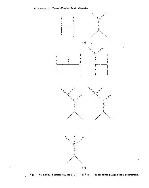
Figure 1: Feynman diagrams: (a) for $e^{+}e^{-}\to W^{+}W^{-}$; (b) for three gauge boson production.

  In ref. BI-TP-90-43 all vector boson self-interaction Lagrangians are expressed in terms of unphysical (unmixed) vector fields $\vec{\tilde{W}},\tilde{Y},\vec{\tilde{V}}$. For calculating physical processes we need the corresponding expressions for the physical fields $W^{\pm},Z,A,V^{\pm},V^{0}$, which can be obtained by appropriately applying the mixing matrices. The resulting expressions are quite lengthy. We summarize them in a fairly compact form (for all interesting vertices) in App. A and B. Similarly, the induced couplings of physical vector bosons to the (unphysical) scalar fields $\vec{\pi}$ and $\vec{\sigma}$ have been calculated, since they will be used in computing some amplitudes for three-boson-production processes (see Fig. 1b), but we won’t quote them here explicitly.

  Note that the approach of refs. BI-TP-88/32 and BI-TP-90-43 to separate systematically the cutoff-dependent one-loop effects into nonobservable (“renormalization”) and observable effects is based on the interpretation of effective theories as first clearly promoted by Appelquist et al. YTP-80-01 . However, other interpretations and handling of effective theories may enjoy equal legitimacy. For example, Casalbuoni et al. UGVA-DPT-1986-01-492 ; CERN-TH-4876/87 ; hep-ph/9303201 take the point of view that there are no quantum-induced terms in the BESS effective theory, but that all terms should be treated as phenomenological parameters. In addition, these authors consider for the BESS the same one-loop radiative corrections as in SM and equate $\Lambda=M_{H}\sim 1$ TeV. This interpretation leads to a somewhat different BESS model than the BESS model discussed here, with the differences ocurring at the one-loop level.

  III Phenomenology

  Present $e^{+}e^{-}$-colliders like LEP I allow only direct tests of the couplings between gauge bosons and fermions. But, as we have shown, the nonrenormalizable structure of the BESS model shows up most drastically in the self-couplings of the gauge bosons due to the new induced couplings. Future $e^{+}e^{+}$-colliders with energies above the $W^{+}W^{-}$ threshold (161 GeV) will allow direct tests of these self-couplings. The first machine to make the W-pair production process $e^{+}e^{-}\to W^{+}W^{-}$ possible will be LEP II ($\sqrt{s}\sim 190\ {\rm GeV}$), but due to its very limited energy range, deviations from the standard model will hardly be observable. A planned $e^{+}e^{-}$ (linear) collider at $\sqrt{s}=500\ {\rm GeV}$ (NLC) will allow much more precise measurements of the $e^{+}e^{-}\to W^{+}W^{-}$ cross section and, in particular, a much better discrimination of the BESS model because of the expected higher integrated luminosity of $20fb^{-1}$ per year Leenen and because the CM energy of $500\ {\rm GeV}$ is much larger than the threshold of this reaction, so that at this energy the violation of the gauge cancellations due to the induced couplings in the BESS model yields much higher deviations from the standard model than at LEP II energies. Furthermore, three gauge boson production processes like $e^{+}e^{-}\to W^{+}W^{-}Z$ and $e^{+}e^{-}\to W^{+}W^{-}\gamma$ MAD/PH/420 ; UCD-88-24 , which supply a direct test of the quartic vector boson self-couplings and the non-Yang–Mills structure of these in the BESS model, will be measurable. The $e^{+}e^{-}\to W^{+}W^{-}Z$ threshold is at $250\ {\rm GeV}$ and the high luminosity will enable even the measurement of very small cross sections in the order of $50fb$ as they are expected for these processes.

  Future hadron colliders and $\gamma\gamma$-collisions at NLC will as well supply tests of vector boson self-interactions and of the induced couplings in the BESS model, but these are not considered in the present analysis.

  In this paper we present the cross sections for the two and three gauge boson production processes at NLC energy of $\sqrt{s}=500\ {\rm GeV}$. In addition, we give an outlook to what happens at an energy of $\sqrt{s}=2000\ {\rm GeV}$, which may be interesting for machines of future generations.

  Specifically, we have calculated the following observables:

• - Total cross sections for the reactions $e^{+}e^{-}\to W^{+}W^{-},e^{+}e^{-}\to W^{+}W^{-}Z$ and $e^{+}e^{-}\to W^{+}W^{-}\gamma$ both for polarized and nonpolarized gauge bosons.

• - The following partial cross sections (distributions):

  • $\bullet$ $d\sigma/d\cos\theta_{G}$ for two and three gauge boson production $(G=W,Z,\gamma)$,

  • $\bullet$ $d\sigma/dE_{G}$ for three gauge boson production,

  • $\bullet$ $d\sigma/dP_{G,T}$ for three gauge boson production,

  • $\bullet$ $d\sigma/dy_{G}$ for three gauge boson production.

• -For the reaction $e^{+}e^{-}\to ZZZ$ we have calculated only the total cross section, since distributions will presumably not be measurable because of the small size of the cross sections.

To identify the gauge boson production events in experiment, one has to reconstruct the W and Z bosons from their decay products, while the photons can be identified directly. As Frank, Mättig, Settles and Zeuner FMSZ have stated, the most significant $e^{+}e^{-}\to W^{+}W^{-}$ events are those, where one W decays into leptons and the other one into hadrons. An analysis of the angular distribution of the decay products of the W and Z bosons yields the polarisation of these bosons, so that the cross section for the production of polarized gauge bosons can be measured, too.

Figures 1a and b show schematically the tree level Feynman diagrams which contribute to the two and three gauge boson production processes. (Since we performed our calculations in the Landau gauge, there is one diagram with an exchange of an unphysical would-be Goldstone boson.) We formally calculated the cross sections at tree level, but for each gauge boson self-interaction vertex we took into account the one-loop induced coupling. All cross sections acquire contributions from cubic self-couplings, whereas in the three gauge boson production processes even quartic self-couplings get involved due to the last diagram. In the case of $e^{+}e^{-}\to ZZZ$ there is a diagram with a coupling of four neutral gauge bosons which does not exist for pure Yang-Mills type interactions, but exists in the BESS model as a consequence of the violation of the Yang-Mills structure.

To calculate the cross section for the W pair production we have proceded completely analytically using the usual trace techniques. For the calculation of the three gauge boson production cross sections we had to procede numerically. We calculated the amplitudes using helicity techniques MAD/PH/420 ; DESY 85/133 and integrated numerically over the phase space. In agreement with MAD/PH/420 we imposed the following transverse-momentum and pseudorapidity cuts on the photon produced in $e^{+}e^{-}\to W^{+}W^{-}\gamma$:

$$P_{T,\gamma}>20\ {\rm GeV},~{}~{}~{}~{}|\eta_{\gamma}|<2.$$

In order to obtain numerical values for the cross sections in the BESS model, we had to specify the free parameters of the model, i.e., $g$,$g^{\prime}$ and $g^{\prime\prime}$, $f^{2}$, $\lambda^{2}$ and the cut-off $\Lambda$. $\Lambda$ was set to

$$\Lambda=5\ {\rm TeV}$$

We are aware that this value may be too large, because the two-loop contributions may become dominant for such a choice, as mentioned before. However, a different choice of $\Lambda$, e.g., $\Lambda=2$ TeV, would change the values of the deviations from SM by only a few per cent. This is due to the fact that only parts of these deviations are due to the one-loop induced couplings, while the larger part stems from tree level effects (existence of heavy gauge bosons, gauge boson mixing). The other five parameters can be determined from chosen values of $\alpha_{\rm em}$, $M_{W}$, $M_{Z}$, $M_{V_{0}}$ and $g^{\prime\prime}/g$. The first three values are empirically given (the electromagnetic fine structure constant $\alpha_{\rm em}$ was taken as 1/127, which is the value of the running coupling constant at the $e^{+}e^{-}\to W^{+}W^{-}Z$ threshold of 250 GeV.) while the free parameter $g^{\prime\prime}/g$ was set to

$$g^{\prime\prime}/g=10,$$

a value suggested by the apparent success of SM in fermionic processes. For the unknown mass $M_{V^{0}}$ we chose the following reference values:

$$M_{V^{0}}=400\ {\rm GeV},~{}~{}1000\ {\rm GeV},~{}~{}2000\ {\rm GeV},{}~{}~{}2500\ {\rm GeV},$$

which indicate the presumable range within which $M_{V^{0}}$ is expected to lie. Remember that $\lambda^{2}$ grows with $M_{V^{0}}$, so a heavy $\rm V^{0}$ means strong induced couplings.

As a further input for our calculation we need the $\rm V^{\pm}$ and $\rm V^{0}$ widths. We calculated these widths taking the induced couplings fully into account. The main decay channels are two and three gauge bosons and fermion pairs. This will be discussed in detail in a forthcoming paper BI-TP-90/14 . Here in Table 1 we only present the results for our reference values. Note that for both $\rm V^{\pm}$ and $V^{0}$, the width is dominated by the two-vector channels and increases strongly with $M_{V}$, such that masses of $M_{V}\stackrel{{\scriptstyle>}}{{\sim}}2200\ {\rm GeV}$ are unlikely. In this respect the reference mass $M_{V^{0}}=2500\ {\rm GeV}$ has to be considered as an extreme case.

Table 1: Widths of the $V$ bosons.

$\lambda^{2}$	$M_{V^{0}}({\rm GeV})$	$\Gamma_{V^{0}}({\rm GeV})$	$M_{V^{\pm}}({\rm GeV})$	$\Gamma_{V^{\pm}}({\rm GeV})$
0.241	400	0.829	399.5	0.748
1.505	1000	31.17	999.0	38.54
6.012	2000	2300	1997.3	1138
9.406	2500	31197	2496.7	23093

For comparison we calculated the cross sections for the standard model as well. Thereby we neglected all Higgs boson effects, which makes sense if the Higgs boson is lighter than $2M_{W}$ or heavier than $\sqrt{s}-M_{Z}$ because then the Higgs boson yields only a negligible contribution. Else, the Higgs boson would show up as a resonance in the $W^{+}W^{-}$ channel and can be identified by a Jacobian Peak in the energy spectrum of the produced $Z$ bosons. So Higgs boson effects can easily be distinguished from effects of the induced couplings in the BESS model.

One further remark is in order here: In calculating the various cross sections in the way described above (tree level diagrams including one-loop induced couplings) we have not included the finite (cutoff-independent) one-loop corrections, although they are not much smaller in size than the induced (cutoff-sensitive) contributions, at least as long as the cutoff is of reasonable size (1-5 TeV). However, these cutoff-independent corrections are expected to be almost the same as the corresponding finite (one-loop) corrections within SM (calculated within that specific renormalization scheme which corresponds to the replacement $1/(4-d)\mapsto\ln(\Lambda/M_{W})=\ln(M_{H}/M_{W})$). The only difference stems from the diagrams with heavy boson lines and is numerically suppressed relative to the typical SM corrections by (powers of) $(M_{W}/M_{V})^{2}$ or $(M_{W}/M_{H})^{2}$. Therefore, the difference between the BESS and the SM results (at one-loop level) is practically insensitive to the finite corrections since they are almost the same for both.

We note here that the production of the BESS resonances at $e^{+}e^{-}$ linear colliders has recently been studied also by Casalbuoni et al. hep-ph/9303201 . Furthermore, an analysis in the latter work, based on the LEP data communicated at the Dallas Conference (1992), yields the free parameter $(g^{\prime\prime}/g)\geq 14-17$, depending on the mass of the top quark being 180 or 150 GeV (when their phenomenological parameter $b$ is set equal to zero). Choosing these larger values for $(g^{\prime\prime}/g)$, instead of the chosen $(g^{\prime\prime}/g)=10$, the deviations from SM calculated in the present paper would certainly become smaller. However, we have to stress that the BESS model considered and analyzed by the authors of ref. hep-ph/9303201 is somewhat different from the BESS model considered here; above all due to the different treatment and interpretation of the quantum one-loop effects, as already mentioned at the end of Sec. II. Actually, the authors of ref. hep-ph/9303201 treat the coefficients of the possible (induced) terms as unspecified parameters, and in their detailed analysis they set most of them equal to zero. We believe that, when incorporating all possible parameters as freely adjustable, the resulting bounds on $(g^{\prime\prime}/g)$ would be considerably different. In any case, it is our experience that the bounds on $(g^{\prime\prime}/g)$, when determined within our scenario (i.e., by taking our values for the indicated parameters), turn out to be different (see ref. BI-TP-90-40 ). Therefore, we do not take the values of ref. hep-ph/9303201 as stringent.

IV Discussion of Numerical Results

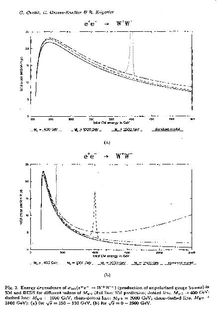
Figure 2: Energy dependence of $\sigma_{tot}(e^{+}e^{-}\to W^{+}W^{-})$ (production of unpolarizedgauge bosons) in SM and BESS for different values of $M_{V^{0}}$ (full line: SM prediction; dotted line: $M_{V^{0}}=400\ {\rm GeV}$; dashed line: $M_{V^{0}}=1000\ {\rm GeV}$; chaindotted line: $M_{V^{0}}=2000\ {\rm GeV}$; chaindashed line: $M_{V^{0}}=2500\ {\rm GeV}$); (a) for $\sqrt{s}=150-550\ {\rm GeV}$; (b) for $\sqrt{s}=0-2500\ {\rm GeV}$.

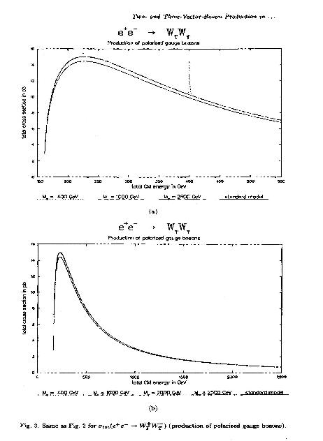
Figure 3: Same as Fig. 2 for $\sigma_{tot}(e^{+}e^{-}\to W^{+}_{T}W^{-}_{T})$ (production of polarized gauge bosons).

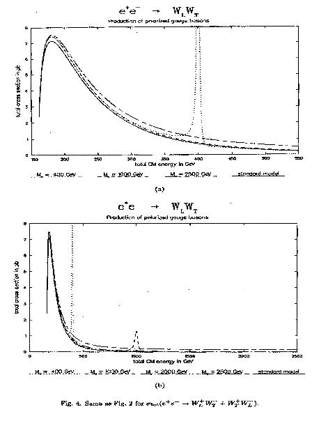
Figure 4: Same as Fig. 2 for $\sigma_{tot}(e^{+}e^{-}\to W^{+}_{L}W^{-}_{T}+W^{+}_{T}W^{-}_{L})$.

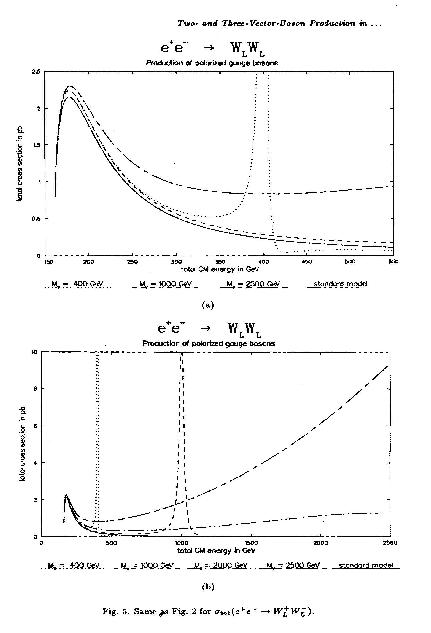
Figure 5: Same as Fig. 2 for $\sigma_{tot}(e^{+}e^{-}\to W^{+}_{L}W^{-}_{L})$.

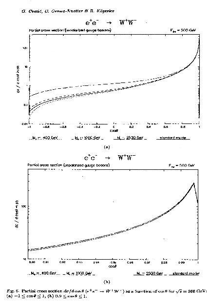
Figure 6: Partial cross section $d\sigma/d\cos\theta(e^{+}e^{-}\to W^{+}W^{-})$ as a function of $\cos\theta$ for $\sqrt{s}=500\ {\rm GeV}$: (a) $-1\leq\cos\theta\leq 1$; (b) $0.9\leq\cos\theta\leq 1$.

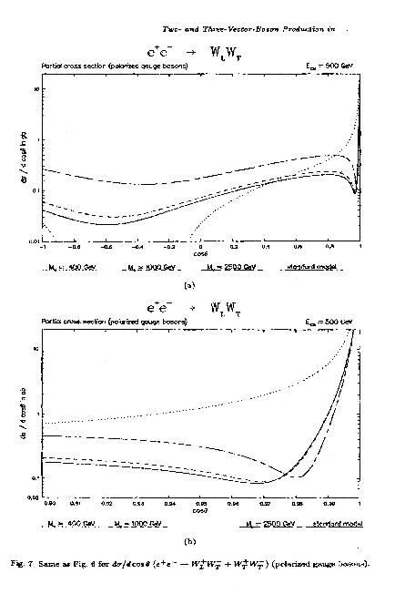
Figure 7: Same as Fig. 6 for $d\sigma/d\cos\theta(e^{+}e^{-}\to W^{+}_{L}W^{-}_{T}+W^{+}_{T}W^{-}_{T})$ (polarized gauge bosons).

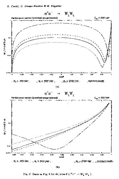
Figure 8: Same as Fig. 6 for $d\sigma/d\cos\theta(e^{+}e^{-}\to W^{+}_{L}W^{-}_{L})$.

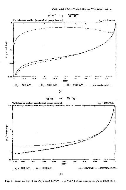
Figure 9: Same as Fig. 6 for $d\sigma/d\cos\theta(e^{+}e^{-}\to W^{+}W^{-})$ at an energy of $\sqrt{s}=2000\ {\rm GeV}$.

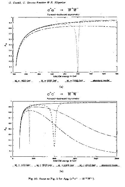
Figure 10: Same as Fig. 2 for $A_{FB}(e^{+}e^{-}\to W^{+}W^{-})$.

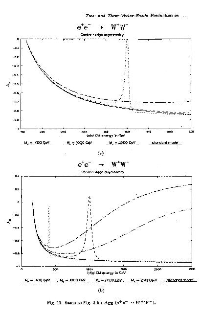
Figure 11: Same as Fig. 2 for $A_{CE}(e^{+}e^{-}\to W^{+}W^{-})$.

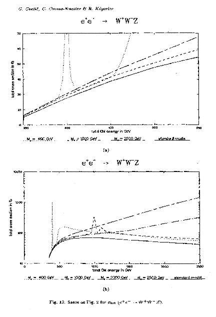
Figure 12: Same as Fig. 2 for $\sigma_{tot}(e^{+}e^{-}\to W^{+}W^{-}Z)$.

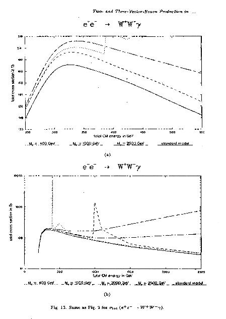
Figure 13: Same as Fig. 2 for $\sigma_{tot}(e^{+}e^{-}\to W^{+}W^{-}\gamma)$.

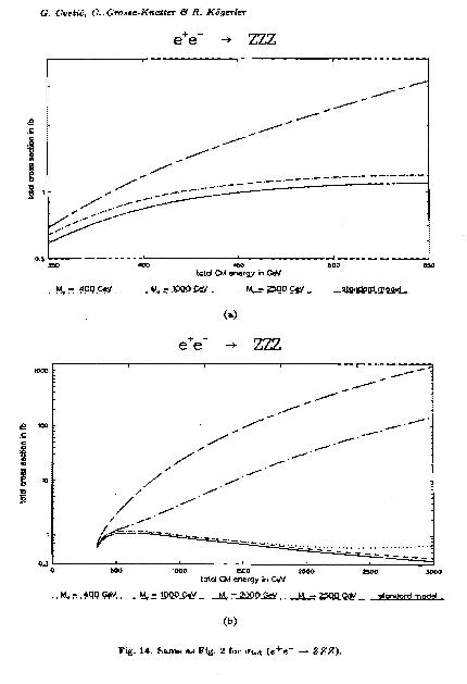
Figure 14: Same as Fig. 2 for $\sigma_{tot}(e^{+}e^{-}\to ZZZ)$.

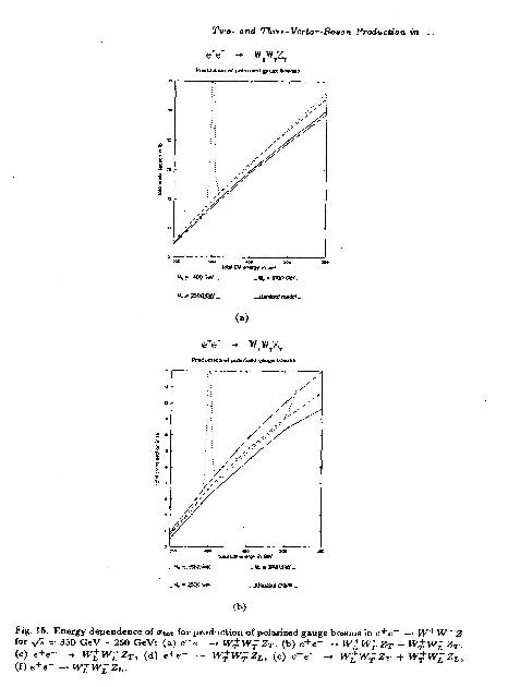
Figure 15: Energy dependence of $\sigma_{tot}$ for production of polarized gauge bosons in $e^{+}e^{-}\to W^{+}W^{-}Z$ for $\sqrt{s}=350-250\ {\rm GeV}$: (a) $e^{+}e^{-}\to W^{+}_{T}W^{-}_{T}Z^{~{}}_{T}$; (b) $e^{+}e^{-}\to W^{+}_{L}W^{-}_{T}Z^{~{}}_{T}+W^{+}_{T}W^{-}_{L}Z^{~{}}_{T}$; (c) $e^{+}e^{-}\to W^{+}_{L}W^{-}_{L}Z^{~{}}_{T}$; (d) $e^{+}e^{-}\to W^{+}_{T}W^{-}_{T}Z^{~{}}_{L}$; (e) $e^{+}e^{-}\to W^{+}_{L}W^{-}_{T}Z^{~{}}_{L}+W^{+}_{T}W^{-}_{L}Z^{~{}}_{L}$; (f) $e^{+}e^{-}\to W^{+}_{L}W^{-}_{L}Z^{~{}}_{L}$.

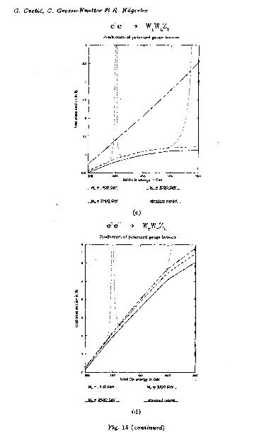
Figure 16: (Fig. 15 continued: Figs. 15c,d)

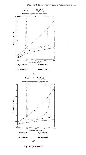
Figure 17: (Fig. 15 continued: Figs. 15e,f)

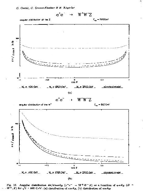
Figure 18: Fig. 16: Angular distribution $d\sigma/d\cos\theta_{B}(e^{+}e^{-}\to W^{+}W^{-}Z)$ as a function of $\cos\theta_{B}\break(B=W^{+},Z)$ for $\sqrt{s}=500\ {\rm GeV}$: (a) distribution of $\cos\theta_{Z}$; (b) distribution of $\cos\theta_{W}$.

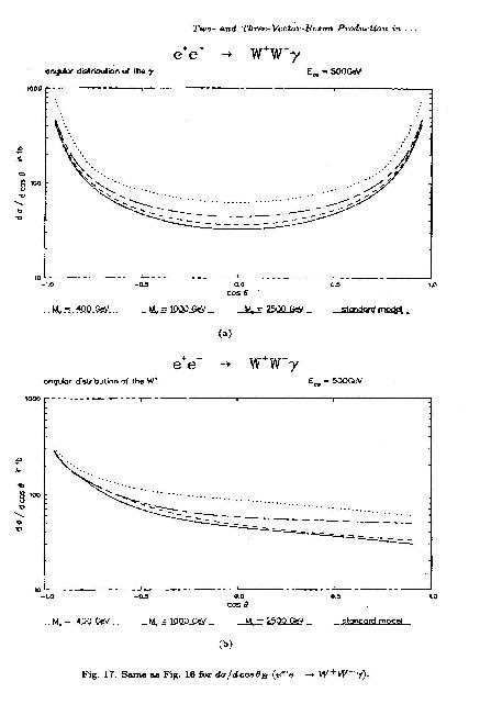
Figure 19: Fig. 17: same as Fig. 16 for $d\sigma/d\cos\theta_{B}(e^{+}e^{-}\to W^{+}W^{-}\gamma)$.

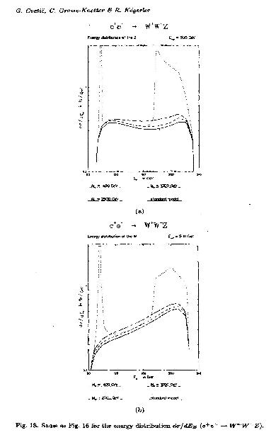
Figure 20: Fig. 18: same as Fig. 16 for the energy distribution $d\sigma/dE_{B}(e^{+}e^{-}\to W^{+}W^{-}Z)$.

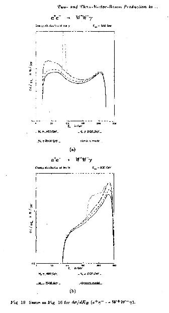
Figure 21: Fig. 19: same as Fig. 16 for $d\sigma/dE_{B}(e^{+}e^{-}\to W^{+}W^{-}\gamma)$.

The results for the different observables (cross sections, distributions, asymmetries) are plotted in Figures 2-21. In all figures the solid lines represent the results for the Higgsless standard model and the different types of broken lines the predictions of the BESS model for different choices of $M_{V^{0}}$, i.e., for different strengths of the induced couplings.

IV.1 ${\bf W^{+}W^{-}}$-Production

In Figs. 2-5 we have depicted the resulting values of the total cross section for $e^{+}e^{-}\to W^{+}W^{-}$ respectively by the BESS model (together with the SM-predictions) for different polarization states of the final vector bosons (unpolarized, transversally (TT), longitudinally (LL) and mixed polarized (LT + TL) $W$’s). We plot the cross sections for two energy intervals:

$${\rm(a)}\;\>\sqrt{s}=150-550\ {\rm GeV}$$

(which covers the energy region to be reached by the planned NLC) and

$${\rm(b)}\;\;\sqrt{s}=0-2500\ {\rm GeV}$$

(which roughly represents the total energy region where the BESS model is reasonably assumed to work).

We have used the $M_{V^{0}}$-values as specified in ch. 3 ($M_{V^{0}}=400,1000,2000,2500\ {\rm GeV}$) for the wide energy range (4.2), whereas, for clarity of presentation, only three $M_{V^{0}}$-values ($M_{V^{0}}=400,1000,2500\ {\rm GeV}$) were used for the narrow (NLC-) energy range a).

Differential cross sections $d\sigma/d\cos\theta$ at $\sqrt{s}=500\ {\rm GeV}$, for non-polarized, (LT- and TL-polarized and LL-polarized $W$’s are depicted in Figs. 6-8 for the angular range $-1\leq\cos\theta\leq+1$ (a). In each case, we isolated in addition the forward direction ($0.9\leq\cos\theta\leq 1$) (b) since, in general, the cross sections are particularly large in this region and, furthermore, the deviations from SM show a substantial variation there. For comparison, we also quoted $d\sigma/d\cos\theta$ at $\sqrt{s}=2000\ {\rm GeV}$ (Fig. 9) for unpolarized vector bosons and for the same two angular regions. The related forward-backward asymmetries $A_{FB}$ and centre-edge asymmetries $A_{CE}$ for unpolarized $W$’s are depicted in Figs. 10 and 11, again for the same two energy ranges as for the total cross sections.

Let us now comment on all these results, in particular on the differences between SM and BESS model predictions.

The deviations from SM stem from three effects:

• a) exchange of heavy boson $V^{0}$ (including the resulting resonance effects),

• b) mixing between light and heavy bosons,

• c) deviations of the $Z^{0}W^{+}W^{-}$ and $\gamma W^{+}W^{-}$ couplings strengths from those of SM due to induced interactions which result in violation of gauge cancellation between $t$ and $s$ channels.

For $\sqrt{s}=500\ {\rm GeV}$ and $M_{V}$ in the range $700\ {\rm GeV}\stackrel{{\scriptstyle<}}{{\sim}}M_{V}\stackrel{{\scriptstyle<}}{{\sim}}1500\ {\rm GeV}$, the largest contribution comes from the tree level effects (a) and (b).

For $M_{V^{0}}\stackrel{{\scriptstyle<}}{{\sim}}1000\ {\rm GeV}$, the $V^{0}$-resonance is narrow and pronounced. For heavy $V^{0}$ ($M_{V^{0}}\stackrel{{\scriptstyle>}}{{\sim}}2000\ {\rm GeV})$, the $V^{0}$-resonance peak becomes very broad, in fact invisible, but the induced couplings are then large and yield large deviations from SM. For instance, at $\sqrt{s}=500\ {\rm GeV}$, the relative deviations of the total cross section (for non-polarized $W$’s) are 3 %, 5%, 8%, 17 % for $M_{V^{0}}=400,1000,2000,2500\ {\rm GeV}$, respectively. Such deviations should therefore be observable with a $500~{}{\rm GeV}~{}e^{+}e^{-}$ collider reaching a luminosity of $20~{}fb^{-1}$ per year where an experimental error smaller than 3 % should be possible (the statistical error for 90 % confidence level being very small $(\sim 0.8\%)$ for a one year’s collection of data. These relative deviations are much more pronounced for L-T polarized $W$’s (5,7 %, 11.3 %, 34 %, 104 %, respectively; statistical error is about 3.5 %) and especially for L-L polarized $W$’s (-43 %, 44 %, 164 %, 560 %, respectively; statistical error is about 5.5 %). On the other hand, for T-T polarized $W$’s, the deviations are practically independent of $M_{V^{0}}$ (about 4 %; statistical error being roughly equal to that of the case of nonpolarized W’s).

From Figs. 10 and 11 we see that the deviations of $A_{FB}$ and $A_{CE}$ at $\sqrt{s}=500\ {\rm GeV}$ are small ($\sim 1-2\%$ for $M_{V^{0}}<1000\ {\rm GeV}$) but will increase drastically with higher energies.

Figs. 6a,b show that the relative deviations of $d\sigma/d\cos\theta$ from SM values at $\sqrt{s}=500\ {\rm GeV}$ for non-polarized $W$’s are substantial for negative values of $\cos\theta$ (e.g. at $\cos\theta=-0.5$ they are - 14 %, + 18 %, + 200 % for $M_{V^{0}}=400,1000,2500\ {\rm GeV}$). However, the absolute values of the cross sections are very small at such angles and the statistical errors are therefore large ($\sim 14.5\%$ for $\Delta(\cos\theta)\approx 0.1$). On the other hand, the deviations in the forward region $(\cos\theta=0.9-0.99)$ are approximately 4 % - 6 % for any $M_{V^{0}}$. The statistical error here is small (about 1 % for $\Delta(\cos\theta)=0.09$). Hence, it appears that it may be more promising to measure $\Delta(d\sigma/d\cos\theta)_{NP}$ in the forward directions than in other directions. The relative deviations are substantially larger for LT + TL channel ($\sim 30-45\%$ for $\cos\theta=-0.5$ and $\sim 1.5\%$ for $\cos\theta=0.9,~{}M_{V^{0}}=400,1000\ {\rm GeV}$). However, the corresponding statistical errors under the mentioned conditions are also large ($\sim 45\%$ and $10\%$, respectively) due to small absolute values. These features (large deviations from SM but large small total cross-sections and large statistical errors) are even more pronounced in the case of LL polarization. Hence it appears that differential cross sections for polarized W’s are not particularly useful quantities for discriminating modes, due to large statistical errors.

As seen from Figs. 9 a and b, $(d\sigma/d(\cos\theta))$ values are drastically decreased at high energies $(\sqrt{s}=2000\ {\rm GeV})$.

IV.2 Three Gauge Boson Production

Figs. 12-14 show the total cross sections for the reactions $e^{+}e^{-}\to W^{+}W^{-}Z,~{}e^{+}e^{-}\to W^{+}W^{-}\gamma$ and $e^{+}e^{-}\to ZZZ$ (all vector bosons unpolarized) as functions of the total energy $\sqrt{s}$, where $\sqrt{s}$ varies again in the two ranges (4.1) and (4.2). Let us first discuss the larger region (4.2) which shows the global behaviour of the cross sections. In addition to the resonance peaks at $\sqrt{s}=M_{V^{0}}$ (due to the exchange of a $V^{0}$ boson in the $s$ channel) which also occur in two body productions, there are $V^{0}$ resonances in the $W^{+}W^{-}$ sub-channel and $V^{\pm}$ resonances in the $W^{\pm}Z$ sub-channel (see Fig. 16) (for $e^{+}e^{-}\to W^{+}W^{-}Z$ and similar for $e^{+}e^{-}\to W^{+}W^{-}\gamma$, but not for $e^{+}e^{-}\to ZZZ$, because there are no diagrams with trilinear couplings). This means that e.g. the direct $e^{+}e^{-}\to W^{+}W^{-}Z$ reaction becomes superimposed by the reactions $e^{+}e^{-}\to V^{0}Z$ with consequent decay $V^{0}\to W^{+}W^{-}$ and by the reaction $e^{+}e^{-}\to V^{\pm}W^{\mp}$ with the decay $V^{\pm}\to W^{\pm}Z$. So above the threshold of these reactions, i.e., at slightly larger energies than the $V^{0}$ resonance, the cross section shows again a maximum. When $M_{V^{0}}$ gets larger, all $V$-resonances broaden (see table 1) and finally dissapear when the $V$-boson width is in the order of or greater than the $V$ boson mass.

An important effect of the induced couplings, as in the case of $W$ pair production, consists in destroying the gauge cancellations, i.e., the parts of the amplitudes for the different graphs which grow with energy do not cancel completely anymore as they would do in a renormalizable gauge theory. This leads to deviations of the BESS model cross sections from the standard model ones, which grow both with energy and with $M_{V^{0}}$, (since $M_{V^{0}}$ is proportional to the strength of the induced couplings). Note that this effect is more pronounced for triple boson production as compared to $W^{+}W^{-}$ production since the induced quartic couplings go with a higher power of $\lambda^{2}$.

At NLC energies (4.1) the deviations from SM are not so drastic, because the non cancelled parts of the amplitudes, which grow with the energy, are still not so big. Except for the case of a very light $V$-boson, which causes resonances at low energies, there are only deviations in the per cent region. (In case of $e^{+}e^{-}\to W^{+}W^{-}Z$ from 8 % for medium $M_{V^{0}}$ up to 20 % for heavy $M_{V^{0}}$.) However, these deviations are large enough to be measurable. The $e^{+}e^{-}\to W^{+}W^{-}Z$ cross section is about 50 fb. With an expected NLC-luminosity of $20fb^{-1}a^{-1}$ there are 1000 annual events. Following the analysis of Barger, Han and Phillips MAD/PH/420 , 20 % of them, that means 200 events per year, will be reconstructable, which means that the statistical error (for 90 % confidence level) can be suppressed to $\sim 5\%$ after five years of run. The systematical error is expected to be 2 % . Thus it should in principle be possible to distinguish the BESS model with the given parameters from the standard model empirically. The same is true for the reaction $e^{+}e^{-}\to W^{+}W^{-}\gamma$. On the other hand, the cross section for the reaction $e^{+}e^{-}\to ZZZ$ is only 1fb, which means the statistical error is probably too large to get precise results, in reasonable time, although this reaction would be of largest importance because of its singular nature.

Figure 15 shows the cross sections for the production of polarized gauge bosons in the reaction $e^{+}e^{-}\to W^{+}W^{-}Z$. The differences of the BESS model to the standard model are small if no or only one longitudinally polarized gauge boson is produced and they are large if two or three longitudinally polarized gauge bosons are produced. This is because the amplitudes of the single Feynman graphs grow with higher powers of $\sqrt{s}$ the more longitudinal bosons are in the final state, so the effect of non-cancellation of the leading powers of $\sqrt{s}$ is especially strong if mainly longitudinal gauge bosons are produced. Unfortunately, in those cases the total cross sections are very small and so the statistics are very bad, while if transversal gauge bosons are produced, the statistics are better because of the larger cross sections but the deviations are small.

Figures 16 to 21 show different partial cross sections at the NLC energy of 500 GeV. Except for resonance effects (in case of a light $V^{0}$) like Jacobian peaks the deviation of the BESS model from the SM results are distributed regularly over the angular, energy etc. region. Thus, a measurement of only those processes where one of the produced gauge bosons is emitted in a certain part of its phase space would not improve the expected deviation from the standard model, but it would make statistics worse because there are less events.

V Conclusions

The discussion of the last section has shown that the specific structures of the BESS model (existence of heavier vector bosons, mixing between heavy and light ones, new induced couplings) will become effective in boson production by $e^{+}e^{-}$-collisions at energies of about 500 GeV with sufficient magnitude, such that an identification of these effects (and, consequently discrimination of BESS and SM) would be possible with the help of the planned New Linear Collider (NLC). The most promising observables in this respect are total cross sections for production of unpolarized and longitudinally polarized gauge bosons. Further valuable information can also be obtained by measuring asymmetries and partial cross sections although the results will be less conclusive due to limited statistics.

In general, quantities connected with two boson production will be measurable to much greater accuracy and yield more distinctive bounds. But results for three boson production processes will be of particular theoretical interest because they are determined partially by the four-boson self-interactions which are much more sensitive to the specific model than the three-vector vertices.

If no deviations from SM will be found in future measurements of the above-mentioned process the results will nevertheless allow to restrict the parameter ranges of the BESS model parameters due to finite experimental accuracy. A careful investigation of the corresponding expectations has been published in ref. hep-ph/9212291 .

Appendix A Trilinear gauge boson self-interactions

The one-loop induced interaction Lagrangians containing three unphysical (unmixed) vector boson fields are written down in Table 5 of ref. BI-TP-90-43 . Here we can consistently forget about the terms proportional to $\partial_{\mu}G^{\mu}~{}~{}~{}(G=\vec{W},Y,\vec{V})$ since we work in the Landau gauge. Decomposing the remaining expressions into charge-eigenstates, applying the mixing matrices ${\cal C}$ (for charged vector bosons) and ${\cal N}$ (for neutral ones) (cf. 2.2 and 2.3) and adding the corresponding tree level interactions we get the total Lagrangian for the cubic self interactions of physical vector bosons (tree level and one-loop induced ones). It can be written in a compact form by using the notation

$${W^{\pm}\choose V^{\pm}}\equiv{c_{1}^{\pm}\choose c_{2}^{\pm}}\ ,~{}~{}~{}~{}~{}~{}~{}~{}~{}~{}~{}~{}~{}~{}\left(\begin{matrix}A\cr Z\cr V^{0}\cr\end{matrix}\right)\equiv\left(\begin{matrix}n_{1}\cr n_{2}\cr n_{3}\cr\end{matrix}\right)\ .$$

One obtains

$${\cal L}_{\rm 3gauge~{}bosons} = i\sum^{2}_{a,b=1}\sum^{2}_{i=0}K_{ab,i}\cdot\{(c_{a}^{+})^{\mu}(c_{b}^{+})^{\nu}(n_{i})_{\mu\nu}++[(c_{a}^{-})_{\mu\nu}(c_{b}^{+})^{\mu}-(c_{b}^{+})_{\mu\nu}(c_{a}^{-})^{\mu}](n_{i})^{\nu}\}\qquad\qquad\qquad\qquad(A.2)$$

where

$$K_{ab,i} = 2{\cal C}_{1a}{\cal C}_{1b}[\alpha_{1}{\cal N}_{oi}+\alpha_{6}{\cal N}_{1i}+\alpha_{2}{\cal N}_{2i}]+2{\cal C}_{2a}{\cal C}_{2b}[\alpha_{3}{\cal N}_{oi}+\alpha_{4}{\cal N}_{1i}+\alpha_{7}{\cal N}_{2i}]+$$

$$+({\cal C}_{1a}{\cal C}_{2b}+{\cal C}_{2a}{\cal C}_{1b})[2\alpha_{2}{\cal N}_{1i}+2\alpha_{4}{\cal N}_{2i}+\alpha_{5}{\cal N}_{oi}]\qquad\qquad\qquad\qquad\qquad\qquad\qquad\qquad\;\;\;(A.3)$$

and [we use the notation: $t\equiv[48(4\pi)^{2}]^{-1}\ \ln(\Lambda/M_{W})$]

$$\alpha_{1} = -t{1\over 4}(\lambda^{2}-1)(\lambda^{2}-3)^{2}$$

$$\alpha_{2} = t{1\over 2}(\lambda^{6}-3\lambda^{4}+5\lambda^{2}+1)$$

$$\alpha_{3} = -t(\lambda^{6}-2\lambda^{4}-1)$$

$$\alpha_{4} = \alpha_{3}$$

$$\alpha_{5} = t(\lambda^{6}-5\lambda^{4}+3\lambda^{2}+1)$$

$$\alpha_{6} = -t{1\over 4}(\lambda^{6}+\lambda^{4}-5\lambda^{2}+11)+{1\over{2g^{2}}}$$

$$\alpha_{7} = t\cdot 2(\lambda^{6}-2\lambda^{4}-1)+{2\over{g^{\prime\prime 2}}}\qquad\qquad\qquad\qquad\qquad\qquad\qquad\qquad\qquad(A.4)$$

Appendix B Quadrilinear gauge boson self-interactions

The one-loop induced interaction Lagrangians connecting four (unmixed) vector boson fields can be found in Table 7 of ref. BI-TP-90-43 . They can be inverted into expressions for quartic interactions of the physical bosons by appropriately using the mixing matrices ${\cal C}$ and ${\cal N}$ (cf. (2.2) and (2.3)). Here, we refrain from quoting the full Lagrangian but we list only quartic (physical) vector boson self-couplings (tree level + one-loop induced ones) which contribute to the processes $e^{+}e^{-}\to W^{+}W^{-}Z,~{}~{}e^{+}e^{-}\to W^{+}W^{-}\gamma$ and $e^{+}e^{-}\to ZZZ$.

$${\cal L}_{W^{\pm}W^{\pm}\gamma\gamma}= \sigma_{1}(A^{\mu}A_{\mu})(W^{+\nu}W^{-}_{\nu})+2\sigma_{2}(A^{\mu}A^{\nu})(W^{+}_{\mu}W^{-}_{\nu}) (B.1a)$$

$${\cal L}_{W^{\pm}W^{\pm}\gamma Z}= \sigma_{3}(A^{\mu}Z_{\mu})(W^{+\nu}W^{-}_{\nu})+\sigma_{4}(A^{\mu}Z^{\nu})(W^{+}_{\mu}W^{-}_{\nu}+W^{+}_{\nu}W^{-}_{\mu}) (B.1b)$$

$${\cal L}_{W^{\pm}W^{\pm}\gamma V^{0}}= \sigma_{5}(A^{\mu}V^{0}_{\mu})(W^{+\nu}W^{-}_{\nu})+\sigma_{6}(A^{\mu}V^{0\nu})(W^{+}_{\mu}W^{-}_{\nu}+W^{+}_{\nu}W^{-}_{\mu}) (B.1c)$$

$${\cal L}_{W^{\pm}W^{\pm}ZZ}= \sigma_{7}(Z^{\mu}Z_{\mu})(W^{+\nu}W^{-}_{\nu})+2\sigma_{8}(Z^{\mu}Z_{\mu})(W^{+}_{\mu}W^{-}_{\nu}) (B.1d)$$

$${\cal L}_{W^{\pm}W^{\pm}ZV^{0}}= \sigma_{9}(Z^{\mu}V^{0}_{\mu})(W^{+\nu}W^{-}_{\nu})+\sigma_{10}(Z^{\mu}V^{0\nu})(W^{+}_{\mu}W^{-}_{\nu}+W^{+}_{\nu}W^{-}_{\mu}) (B.1e)$$

$${\cal L}_{ZZZZ}= \sigma_{11}(Z^{\mu}Z_{\mu})(Z^{\nu}Z_{\nu}) (B.1f)$$

$${\cal L}_{ZZZV^{0}}= \sigma_{12}(V^{0\mu}Z_{\mu})(Z^{\nu}Z_{\nu}) (B.1g)$$

It turns out that all couplings of four neutral gauge bosons where at least one of these is a photon are zero. Note also that there are (non-vanishing) interaction terms involving photon fields which individually are not invariant under $U(1)_{em}$. However, since they are obtained from fully invariant expressions (by expansion in power of fields), electromagnetic gauge invariance is established if the appropriate terms (including in general also cubic boson interaction terms) are added.

The coupling constants are given by:

$$\sigma_{1} = 2\{[\beta_{2}{\cal N}_{00}{\cal N}_{10}+\beta_{4}{\cal N}_{10}{\cal N}_{20}+\beta_{11}{\cal N}^{2}_{00}+\beta_{15}{\cal N}_{20}^{2}+\beta_{24}{\cal N}_{00}{\cal N}_{20}+2\beta_{40}{\cal N}_{10}^{2}]{\cal C}^{2}_{11}$$

$$+[\beta_{4}{\cal N}^{2}_{10}+\beta_{8}{\cal N}^{2}_{20}+2\beta_{18}{\cal N}_{10}{\cal N}_{20}+\beta_{26}{\cal N}_{00}{\cal N}_{10}+\beta_{29}{\cal N}_{00}^{2}+\beta_{35}{\cal N}_{00}{\cal N}_{20}]{\cal C}_{11}{\cal C}_{21}$$

$$+[\beta_{8}{\cal N}_{10}{\cal N}_{20}+\beta_{10}{\cal N}_{00}{\cal N}_{20}+\beta_{15}{\cal N}^{2}_{10}+\beta_{20}{\cal N}^{2}_{00}+\beta_{33}{\cal N}_{00}{\cal N}_{10}+2\beta_{42}{\cal N}^{2}_{20}]{\cal C}^{2}_{21}\}\qquad\qquad\;\;\;\;\;\;\;\;\;\;\;\;\;\;\;\;\;\;\;\;\;\;\;\;\;\;(B.2a)$$

$$\sigma_{2} = [\beta_{1}{\cal N}_{00}{\cal N}_{10}+\beta_{3}{\cal N}_{10}{\cal N}_{20}+\beta_{12}{\cal N}^{2}_{00}+\beta_{16}{\cal N}_{20}^{2}+\beta_{25}{\cal N}_{00}{\cal N}_{20}+2\beta_{39}{\cal N}_{10}^{2}]{\cal C}^{2}_{11}$$

$$+[\beta_{3}{\cal N}^{2}_{10}+\beta_{7}{\cal N}^{2}_{20}+2(\beta_{17}+\beta_{19}){\cal N}_{10}{\cal N}_{20}+(\beta_{27}+\beta_{28}){\cal N}_{00}{\cal N}_{10}+\beta_{30}{\cal N}_{00}^{2}+(\beta_{36}+\beta_{37}){\cal N}_{00}{\cal N}_{20}]{\cal C}_{11}{\cal C}_{21}$$

$$+[\beta_{7}{\cal N}_{10}{\cal N}_{20}+\beta_{9}{\cal N}_{00}{\cal N}_{20}+\beta_{16}{\cal N}^{2}_{10}+\beta_{21}{\cal N}^{2}_{00}+\beta_{34}{\cal N}_{00}{\cal N}_{10}+2\beta_{41}{\cal N}^{2}_{20}]{\cal C}^{2}_{21}\qquad\qquad\;\;\;\;\;\;\;\;\;\;\;\;\;\;\;\;\;\;\;\;\;\;\;\;\;\;\;\;\ (B.2b)$$

$$\sigma_{3} = 2\{[\beta_{2}({\cal N}_{01}{\cal N}_{10}+{\cal N}_{00}{\cal N}_{11})+\beta_{4}({\cal N}_{11}{\cal N}_{20}+{\cal N}_{10}{\cal N}_{21})+2\beta_{11}{\cal N}_{00}{\cal N}_{01}+2\beta_{15}{\cal N}_{20}{\cal N}_{21}+\beta_{24}({\cal N}_{01}{\cal N}_{20}+{\cal N}_{00}{\cal N}_{21})$$

$$+4\beta_{40}{\cal N}_{10}{\cal N}_{11}]{\cal C}^{2}_{11}+[2\beta_{4}{\cal N}_{10}{\cal N}_{11}+2\beta_{8}{\cal N}_{20}{\cal N}_{21}+2\beta_{18}({\cal N}_{11}{\cal N}_{20}+{\cal N}_{10}{\cal N}_{21})+\beta_{26}({\cal N}_{01}{\cal N}_{10}+{\cal N}_{00}{\cal N}_{11})$$

$$+\beta_{29}{\cal N}_{00}{\cal N}_{01}+\beta_{35}({\cal N}_{01}{\cal N}_{20}+{\cal N}_{00}{\cal N}_{21})]{\cal C}_{11}{\cal C}_{21}+[\beta_{8}({\cal N}_{11}{\cal N}_{20}+{\cal N}_{10}{\cal N}_{21})\beta_{10}({\cal N}_{01}{\cal N}_{20}+{\cal N}_{00}{\cal N}_{21})$$

$$+2\beta_{15}{\cal N}_{10}{\cal N}_{11}+2\beta_{20}{\cal N}_{00}{\cal N}_{01}+\beta_{33}({\cal N}_{01}{\cal N}_{10}+{\cal N}_{00}{\cal N}_{11})+4\beta_{42}{\cal N}_{20}{\cal N}_{21}]{\cal C}^{2}_{21}\}\qquad\qquad\;\;\;\;\;\;\;\;\;\;\;\;\;\;\;\;\;\;\;\;\;\;\;\;\;\;\;\;(B.2c)$$

$$\sigma_{4} = [\beta_{1}({\cal N}_{01}{\cal N}_{10}+{\cal N}_{00}{\cal N}_{11})+\beta_{3}({\cal N}_{11}{\cal N}_{20}+{\cal N}_{10}{\cal N}_{21})+2\beta_{12}{\cal N}_{00}{\cal N}_{01}+2\beta_{16}{\cal N}_{20}{\cal N}_{21}+\beta_{25}({\cal N}_{01}{\cal N}_{20}+{\cal N}_{00}{\cal N}_{21})$$

$$+4\beta_{39}{\cal N}_{10}{\cal N}_{11}]{\cal C}^{2}_{11}+[2\beta_{3}{\cal N}_{10}{\cal N}_{11}+2\beta_{7}{\cal N}_{20}{\cal N}_{21}+2(\beta_{17}+\beta_{19})({\cal N}_{11}{\cal N}_{20}+{\cal N}_{10}{\cal N}_{21})$$

$$+(\beta_{27}+\beta_{28})({\cal N}_{01}{\cal N}_{10}+{\cal N}_{00}{\cal N}_{11})+2\beta_{30}{\cal N}_{00}{\cal N}_{01}+(\beta_{36}+\beta_{37})({\cal N}_{01}{\cal N}_{20}+{\cal N}_{00}{\cal N}_{21})]{\cal C}_{11}{\cal C}_{21}$$

$$+[\beta_{7}({\cal N}_{11}{\cal N}_{20}+{\cal N}_{10}{\cal N}_{21})+\beta_{9}({\cal N}_{01}{\cal N}_{20}+{\cal N}_{00}{\cal N}_{21})+2\beta_{16}{\cal N}_{10}{\cal N}_{11}$$

$$+2\beta_{21}{\cal N}_{00}{\cal N}_{01}+\beta_{34}({\cal N}_{01}{\cal N}_{10}+{\cal N}_{00}{\cal N}_{11})+4\beta_{41}{\cal N}_{20}{\cal N}_{21}]{\cal C}^{2}_{21}\qquad\qquad\;\;\;\;\;\;\;\;\;\;\;\;\;\;\;\;\;\;\;\;\;\;\;\;\;\;\;\;\;\;\;\;\;\;\;\;\;\;\;\;\;\;\;\;\;\;\;\;\;\;\;\;\ (B.2d)$$

$$\sigma_{11} = (\beta_{1}+\beta_{2}){\cal N}_{01}{\cal N}_{11}^{3}+(\beta_{3}+\beta_{4}){\cal N}_{21}{\cal N}^{3}_{11}+\beta_{5}{\cal N}_{11}{\cal N}^{3}_{01}+\beta_{6}{\cal N}_{21}{\cal N}^{3}_{01}+\beta_{7}+\beta_{8}){\cal N}_{11}{\cal N}^{3}_{21}+(\beta_{9}+\beta_{10}){\cal N}_{01}{\cal N}^{3}_{21}$$

$$+(\beta_{11}+\beta_{12}+\beta_{13}+\beta_{14}){\cal N}^{2}_{01}{\cal N}^{2}_{11}+(\beta_{15}+\beta_{16}+\beta_{17}+\beta_{18}+\beta_{19}){\cal N}^{2}_{11}{\cal N}^{2}_{21}+(\beta_{20}+\beta_{21}+\beta_{22}+\beta_{23}){\cal N}^{2}_{01}{\cal N}^{2}_{21}$$

$$+(\beta_{24}+\beta_{25}+\beta_{26}+\beta_{27}+\beta_{28}){\cal N}_{01}{\cal N}_{21}{\cal N}^{2}_{11}+(\beta_{29}+\beta_{30}+\beta_{31}+\beta_{32}){\cal N}_{11}{\cal N}_{21}{\cal N}^{2}_{01}$$

$$+(\beta_{33}+\beta_{34}+\beta_{35}+\beta_{36}+\beta_{37}){\cal N}_{01}{\cal N}_{11}{\cal N}^{2}_{21}+\beta_{38}{\cal N}^{4}_{01}+(\beta_{39}+\beta_{40}){\cal N}^{4}_{11}+(\beta_{41}+\beta_{42}){\cal N}^{4}_{21}\qquad\;\;\;\;\;\;\;\;\;\;\;\;\;\;\;(B.2e)$$

$$\sigma_{12} = (\beta_{1}+\beta_{2})({\cal N}_{02}{\cal N}_{11}^{3}+3{\cal N}_{01}{\cal N}_{12}{\cal N}^{2}_{11})+(\beta_{3}+\beta_{4})({\cal N}_{22}{\cal N}^{3}_{11}+3{\cal N}_{21}{\cal N}_{12}{\cal N}_{11})+\beta_{5}({\cal N}_{12}{\cal N}^{3}_{01}+3{\cal N}_{11}{\cal N}_{02}{\cal N}^{2}_{01})$$

$$+\beta_{6}({\cal N}_{22}{\cal N}^{3}_{01}+3{\cal N}_{21}{\cal N}_{02}{\cal N}^{2}_{01})+(\beta_{7}+\beta_{8})({\cal N}_{12}{\cal N}^{3}_{21}+3{\cal N}_{11}{\cal N}_{22}{\cal N}^{2}_{21})+(\beta_{9}+\beta_{10})({\cal N}_{02}{\cal N}^{3}_{21}+3{\cal N}_{21}{\cal N}_{22}{\cal N}^{2}_{21})$$

$$+(\beta_{11}+\beta_{12}+\beta_{13}+\beta_{14})({\cal N}_{02}{\cal N}_{01}{\cal N}^{2}_{11}+{\cal N}_{12}{\cal N}_{11}{\cal N}^{2}_{01})$$

$$+2(\beta_{15}+\beta_{16}+\beta_{17}+\beta_{18}+\beta_{19})({\cal N}_{12}{\cal N}_{11}{\cal N}^{2}_{21}+{\cal N}_{22}{\cal N}_{21}{\cal N}^{2}_{11})$$

$$+2(\beta_{20}+\beta_{21}+\beta_{22}+\beta_{23})({\cal N}_{02}{\cal N}_{01}{\cal N}^{2}_{21}+{\cal N}_{22}{\cal N}_{21}{\cal N}^{2}_{01})$$

$$+(\beta_{24}+\beta_{25}+\beta_{26}+\beta_{27}+\beta_{28})({\cal N}_{02}{\cal N}_{21}{\cal N}^{2}_{11}+{\cal N}_{01}{\cal N}_{22}{\cal N}^{2}_{11}+2{\cal N}_{01}{\cal N}_{21}{\cal N}_{12}{\cal N}_{11})$$

$$+(\beta_{29}+\beta_{30}+\beta_{31}+\beta_{32})({\cal N}_{12}{\cal N}_{21}{\cal N}^{2}_{01}+{\cal N}_{11}{\cal N}_{22}{\cal N}^{2}_{01}+2{\cal N}_{11}{\cal N}_{21}{\cal N}_{02}{\cal N}_{01})$$

$$+(\beta_{33}+\beta_{34}+\beta_{35}+\beta_{36}+\beta_{37})({\cal N}_{02}{\cal N}_{11}{\cal N}^{2}_{21}+{\cal N}_{01}{\cal N}_{12}{\cal N}^{2}_{21}+2{\cal N}_{01}{\cal N}_{11}{\cal N}_{22}{\cal N}_{21})$$

$$+4\beta_{38}{\cal N}_{02}{\cal N}^{3}_{01}+4(\beta_{39}+\beta_{40}){\cal N}_{12}{\cal N}^{3}_{11}+4(\beta_{41}+\beta_{42}){\cal N}_{22}{\cal N}^{3}_{21}.\qquad\qquad\;\;\;\;\;\;\;\;\;\;\;\;\;\;\;\;\;\;\;\;\;\;\;\;\;\;\;\;\;\;\;\;\;\;\;\;\;\;\;\;\;\;\;\;\;\;\;\;\;\;\;\;(B.2f)$$

$\sigma_{7}$ can be obtained from the formula for $\sigma_{1}$ and $\sigma_{8}$ from the formula for $\sigma_{2}$ by the substitution ${\cal N}_{i0}\to{\cal N}_{i1}$. $\sigma_{5}$ and $\sigma_{6}$ are constructed from $\sigma_{3}$ and $\sigma_{4}$ respectively replacing ${\cal N}_{i1}\to{\cal N}_{i2}$, to find $\sigma_{9}$ and $\sigma_{10}$ one has to replace ${\cal N}_{i0}\to{\cal N}_{i2}$ in $\sigma_{3}$ and $\sigma_{4}$.

The ${\cal C}_{ij}$ and ${\cal N}_{ij}$ are again the elements of the mixing matrix (2.2) and (2.3) and the $\beta_{i}$ are the couplings of the unmixed gauge bosons [we use the notation: $t\equiv[48(4\pi)^{2}]^{-1}\ \ln(\Lambda/M_{W})$]:

$$\beta_{1} = {1\over 2}t(\lambda^{8}-2\lambda^{6}-2\lambda^{4}+10\lambda^{2}-7)$$

$$\beta_{2} = {1\over 4}t(\lambda^{8}+4\lambda^{6}-26\lambda^{4}+52\lambda^{2}-31)$$

$$\beta_{3} = -{1\over 2}t(2\lambda^{8}-5\lambda^{6}+\lambda^{4}+9\lambda^{2}+1)$$

$$\beta_{4} = -{1\over 2}t(\lambda^{8}-\lambda^{6}-7\lambda^{4}+21\lambda^{2}+2)$$

$$\beta_{5} = {3\over 4}t(\lambda^{8}-10\lambda^{4}+24\lambda^{2}-15)$$

$$\beta_{6} = -{3\over 2}t(\lambda^{8}-2\lambda^{6}-2\lambda^{4}+10\lambda^{2}+1)$$

$$\beta_{7} = -2t(2\lambda^{8}-\lambda^{6}+1)\ ,\qquad\beta_{8}=-2t(\lambda^{8}+\lambda^{6}+2)$$

$$\beta_{9} = \beta_{7}\ ,\qquad\beta_{10}=\beta_{8}$$

$$\beta_{11} = {1\over 8}t(\lambda^{8}-8\lambda^{6}+30\lambda^{4}-40\lambda^{2}+17)$$

$$\beta_{12} = {1\over 4}t(\lambda^{8}+4\lambda^{6}+6\lambda^{4}-28\lambda^{2}+17)$$

$$\beta_{13} = {1\over 4}t(\lambda^{8}-10\lambda^{6}+34\lambda^{4}-42\lambda^{2}+17)$$

$$\beta_{14} = {1\over 2}t(\lambda^{8}+8\lambda^{6}-2\lambda^{4}-24\lambda^{2}+17)$$

$$\beta_{15} = {1\over 2}t(\lambda^{8}-3\lambda^{6}+4\lambda^{4}+\lambda^{2}+1)$$

$$\beta_{16} = t(\lambda^{8}+\lambda^{4}+7\lambda^{2}+1)$$

$$\beta_{17} = {1\over 2}t(2\lambda^{8}-7\lambda^{6}+10\lambda^{4}+\lambda^{2}+2)$$

$$\beta_{18} = {1\over 2}t(2\lambda^{8}+5\lambda^{6}-14\lambda^{4}+13\lambda^{2}+2)$$

$$\beta_{19} = {1\over 2}t(2\lambda^{8}-\lambda^{6}-8\lambda^{4}+\lambda^{2}+2)$$

$$\beta_{20} = \beta_{15}\ ,\quad\beta_{21}=\beta_{16}\ ,\quad\beta_{22}=\beta_{17}\ ,\quad\beta_{23}=\beta_{18}$$

$$\beta_{24} = -{1\over 2}t(\lambda^{8}-3\lambda^{6}+9\lambda^{4}-9\lambda^{2}+2)$$

$$\beta_{25} = -{1\over 2}t(2\lambda^{8}+3\lambda^{6}+3\lambda^{4}-9\lambda^{2}+1)$$

$$\beta_{26} = -t(\lambda^{8}+8\lambda^{6}-13\lambda^{4}+2\lambda^{2}+2)$$

$$\beta_{27} = -{1\over 2}t(2\lambda^{8}+\lambda^{6}-5\lambda^{4}+\lambda^{2}+1)$$

$$\beta_{28} = -{1\over 2}t(2\lambda^{8}-11\lambda^{6}+25\lambda^{4}-17\lambda^{2}+1)$$

$$\beta_{29} = \beta_{24}\ ,\quad\beta_{30}=\beta_{25}$$

$$\beta_{31} = -{1\over 2}t(4\lambda^{8}+17\lambda^{6}-31\lambda^{4}+5\lambda^{2}+5)$$

$$\beta_{32} = \beta_{28}$$

$$\beta_{33} = t(\lambda^{8}+7\lambda^{6}-8\lambda^{4}-\lambda^{2}+1)$$

$$\beta_{34} = 2t(\lambda^{8}-2\lambda^{6}+\lambda^{4}-7\lambda^{2}+1)$$

$$\beta_{35} = t(2\lambda^{8}+3\lambda^{6}+6\lambda^{4}-13\lambda^{2}+2)$$

$$\beta_{36} = t(2\lambda^{8}-3\lambda^{6}+12\lambda^{4}-\lambda^{2}+2)$$

$$\beta_{37} = t(2\lambda^{8}+3\lambda^{6}-6\lambda^{4}-\lambda^{2}+2)$$

$$\beta_{38} = {3\over{16}}t(\lambda^{8}-4\lambda^{6}+6\lambda^{4}-4\lambda^{2}+17)$$

$$\beta_{39} = {1\over 8}t(\lambda^{8}-4\lambda^{6}+2\lambda^{4}+4\lambda^{2}-3)+{1\over{4g^{2}}}$$

$$\beta_{40} = {1\over{16}}t(\lambda^{8}-4\lambda^{6}+14\lambda^{4}-20\lambda^{2}+57)-{1\over{4g^{2}}}$$

$$\beta_{41} = 2t(\lambda^{8}-\lambda^{4})+{1\over{g^{\prime\prime 2}}}$$

$$\beta_{42} = t(\lambda^{8}+2\lambda^{4}+3)-{1\over{g^{\prime\prime 2}}}\qquad\;\;\;\;\;\;\;\;\;\;\;\;\;\;\;\;\;\;\;\;\;\;\;\;\;\;\;\;\;\;\;\;\;\;\;\;\;\;\;\;\;\;\;\;\;\;\;\;\;\;\;\;\;\;\;\;\;\;\;\;(B.3)$$

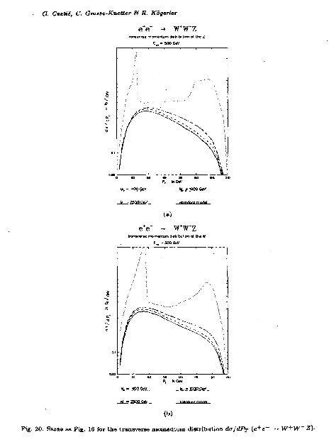
Figure 22: Fig. 20: same as Fig. 16 for the transverse momentum distribution $d\sigma/dP_{T}$ ($e^{+}e^{-}$$\to W^{+}W^{-}Z$).

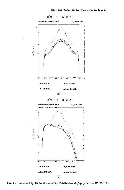
Figure 23: Fig. 21: same as Fig. 16 for the rapidity distribution $d\sigma/dy(e^{+}e^{-}\to W^{+}W^{-}Z)$.

References

• (1) See β€œβ€™e+​eβˆ’superscript𝑒superscript𝑒e^{+}e^{-} Collisions at 500 GeV’ - The Physical Impact,” published in DESY-Report-92-123, ed. P.Β Zerwas, DESY, Hamburg, Germany, 1992; Proceedings of the β€œWorkshop on Physics and Experiments with Linear Colliders”, ed. M.Β Nordberg, SaariselkΓ€, Finnland, 1991.
• (2) For cubic self-interactions a fairly model-dependent analysis based on symmetry considerations has been performed in: G.Β Gounaris, J.Β L.Β Kneur, J.Β Layssac, G.Β Moultaka, F.Β M.Β Renard, D.Β Schildknecht (Bielefeld-Montpellier-Thessaloniki-Collaboration), in Ref.Β Proc1 , p.735 (and: Bielefeld preprint BI-TP 91/40 (1991)); M.Β S.Β Bilenky, J.Β L.Β Kneur, F.Β M.Β Renard and D.Β Schildknecht, β€œTrilinear couplings among the electroweak vector bosons and their determination at LEP-200,” Nucl.Β Phys.Β BΒ 409, 22 (1993).
• (3) R.Β Casalbuoni, S.Β De Curtis, D.Β Dominici and R.Β Gatto, β€œPhysical implications of possible $J=1$ bound states from strong Higgs,” Nucl.Β Phys.Β BΒ 282, 235 (1987); β€œEffective weak interaction theory with possible new vector resonance from a strong Higgs sector,” Phys.Β Lett.Β BΒ 155, 95 (1985).
• (4) G.Β Cvetič and R.Β KΓΆgerler, β€œFermionic couplings in an electroweak theory with nonlinear spontaneous symmetry breaking,” Nucl.Β Phys.Β BΒ 328, 342 (1989); β€œInduced fermionic interactions in theories with general nonlinearly realized SSB,” Z.Β Phys.Β CΒ 48, 109 (1990).
• (5) G.Β Cvetič and R.Β KΓΆgerler, β€œComplete determination of gauge boson selfinteractions in the BESS model,” Nucl.Β Phys.Β BΒ 363, 401 (1991).
• (6) G. Cvetič, C. Grosse-Knetter and R. KΓΆgerler, β€œVector boson selfinteractions and vector boson production within the BESS model,” in Ref.Β Proc1 , p.Β 775 (and Bielefeld preprint BI-TP 91/37 (1991)).
• (7) R.Β BΓΆnisch, C.Β Grosse-Knetter and R.Β KΓΆgerler, β€œBounds on BESS model parameters from vector boson production in e+ e- collisions,” Z.Β Phys.Β CΒ 59, 109 (1993) [hep-ph/9212291].
• (8) A.Β Hosoya and K.Β Kikkawa, β€œQuantum theory of collective motions and an application totTheory of extended hadrons,” Nucl.Β Phys.Β BΒ 101, 271 (1975); J.Β Alfaro and P.Β H.Β Damgaard, β€œField transformations, collective coordinates and BRST invariance,” Annals Phys.Β Β 202, 398 (1990).
• (9) T.Β Kunimasa and T.Β Goto, β€œGeneralization of the Stueckelberg formalism to the massive Yang-Mills field,” Prog.Β Theor.Β Phys.Β Β 37, 452 (1967); T.Β Sonoda and S.Β Y.Β Tsai, β€œThe generalized Stuckelberg formalism and the Glashow-Weinberg-Aalam electroweak model,” Prog.Β Theor.Β Phys.Β Β 71, 878 (1984).
• (10) T.Β Appelquist and C.Β W.Β Bernard, β€œStrongly interacting Higgs bosons,” Phys.Β Rev.Β DΒ 22, 200 (1980); A.Β C.Β Longhitano, β€œLow-energy impact of a heavy Higgs boson sector,” Nucl.Β Phys.Β BΒ 188, 118 (1981); J.Β van der Bij and M.Β J.Β G.Β Veltman, β€œTwo loop large Higgs mass correction to the $\rho$ parameter,” Nucl.Β Phys.Β BΒ 231, 205 (1984).
• (11) M.Β Bando, T.Β Kugo, S.Β Uehara, K.Β Yamawaki and T.Β Yanagida, β€œIs $\rho$ meson a dynamical gauge boson of hidden local symmetry?,” Phys.Β Rev.Β Lett.Β Β 54, 1215 (1985); see also: A.Β P.Β Balachandran, A.Β Stern and C.Β G.Β Trahern, β€œNonlinear models as gauge theories,” Phys.Β Rev.Β DΒ 19, 2416 (1979).
• (12) For two-dimensional theories see: V.Β L.Β Golo and A.Β M.Β Perelomov, β€œSolution of the Duality Equations for the two-dimensional SU(N) invariant Chiral Model,” Phys.Β Lett.Β BΒ 79, 112 (1978); A.Β D’Adda, M.Β LΓΌscher and P.Β Di Vecchia, β€œA $1/n$-expandable series of Nonlinear Sigma Models with instantons,” Nucl.Β Phys.Β BΒ 146, 63 (1978); for three-dimensional theories see: I.Β Y.Β .Arefeva and S.Β I.Β Azakov, β€œRenormalization and phase transition in the Quantum $C_{p}^{n-1}$ Model ($d=2,3$),” Nucl.Β Phys.Β BΒ 162, 298 (1980); for four-dimensional theories see: R.Β KΓΆgerler, W.Β Lucha, H.Β Neufeld and H.Β Stremnitzer, β€œDynamical generation of gauge bosons of hidden local symmetries in Nonlinear Sigma Models,” Phys.Β Lett.Β BΒ 201, 335 (1988); T.Β Kugo, Soryushiron Kenkyu 71, E78 (1985); T.Β Kugo, H.Β Terao and S.Β Uehara, β€œDynamical gauge bosons and hidden local symmetries,” Prog. Theor. Phys. Suppl., No.Β 85, 122-135 (1985).
• (13) R.Β Casalbuoni, P.Β Chiappetta, D.Β Dominici, F.Β Feruglio and R.Β Gatto, β€œHigh-energy tests for a possible strong sector in the standard model,” Nucl.Β Phys.Β BΒ 310, 181 (1988); R.Β Casalbuoni, D.Β Dominici, F.Β Feruglio and R.Β Gatto, β€œTesting the Standard Model in terms of a possible strong scalar sector,” Phys.Β Lett.Β BΒ 200, 495 (1988).
• (14) R.Β BΓΆnisch and R.Β KΓΆgerler, β€œPhenomenological parameter analysis of a Higgsless electroweak gauge theory with induced interactions included,” Int.Β J.Β Mod.Β Phys.Β AΒ 7, 5475 (1992).
• (15) K.Β -i.Β Shizuya, β€œRenormalization of two-dimensional massive Yang-Mills theory and nonrenormalizability of its four-dimensional version,” Nucl.Β Phys.Β BΒ 121, 125 (1977).
• (16) R.Β Casalbuoni, P.Β Chiappetta, A.Β Deandrea, S.Β De Curtis, D.Β Dominici and R.Β Gatto, β€œVector resonances from a strong electroweak sector at linear colliders,” Z.Β Phys.Β CΒ 60, 315 (1993) [hep-ph/9303201].
• (17) M.Β Leenen, talk given at EE500 Workshop (MPI, Munich, Germany, 1992).
• (18) V.Β D.Β Barger, T.Β Han and R.Β J.Β N.Β Phillips, β€œW​W​Zπ‘Šπ‘Šπ‘WWZ, $ZZZ$ and $WW\gamma$ production at $e^{+}e^{-}$ colliders,” Phys.Β Rev.Β DΒ 39, 146 (1989).
• (19) A.Β Tofighi-Niaki and J.Β F.Β Gunion, β€œGeneral amplitudes for three gauge boson production and cross sections and polarization analysis at an $e^{+}e^{-}$ collider,” Phys.Β Rev.Β DΒ 39, 720 (1989).
• (20) M. Frank, P. MΓ€ttig, R. Settles, W. Zeuner, in Ref.Β Proc1 , p.Β 223.
• (21) K.Β Hagiwara and D.Β Zeppenfeld, β€œHelicity amplitudes for heavy lepton production in $e^{+}e^{-}$ annihilation,” Nucl.Β Phys.Β BΒ 274, 1 (1986).
• (22) For first (incomplete) calculation see: G.Β Cvetič, R.Β KΓΆgerler and J.Β TrampetiΔ‡, β€œPhenomenological implications of an electroweak theory without Higgs,” Phys.Β Lett.Β BΒ 248, 128 (1990).
Refer to caption