IFJPAN-IV-2007-4
CERN-PH-TH/2007-064

Markovian Monte Carlo solutions
of the one-loop CCFM equations^⋆

K. Golec-Biernat^ac, S. Jadach^ad, W. Płaczek^b,
P. Stephens^a and M. Skrzypek^ad

^aInstitute of Nuclear Physics IFJ-PAN,
ul. Radzikowskiego 152, 31-342 Cracow, Poland.
^bMarian Smoluchowski Institute of Physics, Jagiellonian University,
ul. Reymonta 4, 30-059 Cracow, Poland.
^cInstitute of Physics, University of Rzeszow,
ul. Rejtana 16A, 35-959 Rzeszow, Poland.
^dCERN, PH Department, CH-1211 Geneva 23, Switzerland.

A systematic extension of the Monte Carlo (MC) algorithm, that solves the DGLAP equation, into the so-called the one-loop CCFM evolution is presented. Modifications are related to a $z$-dependent coupling constant; transverse momentum dependence is added to the $x$-dependence of the parton distributions. The presented Markovian algorithm for one-loop CCFM evolution is the first step in extending it to other more sophisticated schemes beyond DGLAP. In particular, implementing the complete CCFM will be the next step. The presently implemented one-loop CCFM option will be a useful tool in testing the forthcoming MC solutions. Numerical results of the new MC are confronted with other non-MC numerical solutions. The agreement within the MC statistical error of $\sim 0.1\%$ is found. Also, numerical results for $k^{T}$-dependent structure functions are presented.

To be submitted to Acta Physica Polonica

IFJPAN-IV-2007-4
CERN-PH-TH/2007-064

^⋆The project is partly supported by the EU grant MTKD-CT-2004-510126, realized in the partnership with the CERN Physics Department and by the Polish Ministry of Science and Information Society Technologies grant No 620/E-77/6.PR UE/DIE 188/2005-2008.

1 Introduction

The evolution equations (EVEQs) play a crucial role in the construction of any parton shower Monte Carlo program simulating the production of multiple gluons and quarks, in an approximate way, in perturbative QCD. In particular, EVEQs are in this context used to model the actual development of the tree-like cascade of primary emitted partons from the initial hadron. Such a cascade is then supplemented with an appropriate hard scattering matrix element and with the hadronization mechanism to form the complete parton shower MC code.

The basic, and by far the best analyzed, EVEQs in QCD are the DGLAP equations [1]; originally formulated in the leading order, later extended to the next-to-leading order [2, 3, 4, 5] and recently even to the next-to-next-to-leading order [6, 7]. These equations perform systematic resummation in terms of the variable $\log Q$, where $Q$ is a hard scale, for not too small or too large values of the longitudinal momentum fraction $x$.

Another important EVEQ is the BFKL equation [8]. Originally formulated in the leading order, it has been recently extended to the next-to-leading order [9]. Contrary to the DGLAP equations, it resums large $\log x$ terms, therefore, describing the small $x$ limit better than the DGLAP equations. In recent years attempts have been made to improve the DGLAP evolution equations in the small-$x$ region by incorporating some of the BFKL features [10, 11]. However, these attempts have lead to rather complicated evolution equations.

The third class of EVEQs in QCD are the CCFM equations [12]. They are formulated for the so called “unintegrated” parton distributions, which depend on the transverse momenta of partons $k^{T}$ in addition to $x$ and $Q$. The main idea of the CCFM approach is to correctly describe not only the large-$x$ region, where the summation of $\log q$ dominates, but also the region of small $x$, where the large logarithms $\ln(1/x)$ are important. Thus, the CCFM equations effectively interpolate between the DGLAP and BFKL equations. One of the variants of the CCFM equations, called “one-loop” [13], is of special interest because of its simplicity and ease in extending to non-leading orders and to non-gluonic evolutions.

The one-loop CCFM equation combines coherence effects (angular ordering of gluonic emissions) at large $x$ with the transverse momentum ordering at small $x$ [14]. In contrast, the “all-loop” CCFM formulation extends the angular ordering to the small $x$ region. In its original formulation the CCFM scheme has been formulated only for gluonic cascades. In the “one-loop” approximation, as defined in ref. [15], it was extended to include also quarks into it.

Finally, let us mention yet another class of equations, the IREE ones [16], which account for both the logarithms of $Q$ and $x$ by means of constructing and solving the so-called two-dimensional infrared evolution equations.

In a series of recent papers [17, 18, 19, 20, 21, 22, 23, 24, 25], a new family of Monte Carlo algorithms that solve the EVEQs in QCD has been developed. The novelty of these algorithms is in their ability to include an energy constraint on top of the normal Markovian random walk-type evolution. This is of the utmost importance in the case of the MC simulations of narrow resonance production processes initiated by initial state parton cascades. In parallel to the “constrained” algorithms, we have also developed the standard “unconstrained” ones, which are useful for tests and precise studies (for example, for fitting deep-inelastic structure function $F_{2}$). In the very beginning of the above studies, the DGLAP evolution and some of its variants were the main object of the interest. However, from the previous discussion it is clear that it would be useful and interesting to extend them also to other types EVEQs, like those mentioned, having in mind the construction of the parton shower Monte Carlo at a later stage.

In the presented paper we take a first step in that direction and show how the Markovian “unconstrained” DGLAP algorithm can be extended to the one-loop CCFM case. This extension involves two steps: the modification of the coupling constant which becomes $z$-dependent and the inclusion of transverse momenta into the evolution.

In the subsequent papers further extensions of the Markovian algorithms will be presented, in particular to the all-loop CCFM scheme. All technical aspect of the implementation of these “constrained” MC algorithms are discussed at length in ref. [26]. Summarizing, this work should be be treated as a warm-up exercise for the forthcoming more complete and also more sophisticated analysis.

The paper is organized as follows. In Section 2 we recall some basic formulae on the DGLAP equations and describe in detail problems to be solved. Section 3 is devoted to the changes in the algorithm related to the modification of the argument of the coupling constant. Section 4 describes the extension of the algorithm to the $k^{T}$-dependent evolution. In Section 5 some numerical results are presented, and finally, Section 6 contains summary and outlook.

2 Framework

In this paper we will heavily rely on the notation and formulas from [23] where the reader will find more details on the notation and description of the framework which we use. We start from the DGLAP equations

$$\partial_{t}\,xD_{K}(t,x)=\sum_{J}\int\limits_{x}^{1}\frac{dz}{z}\;z\mathcal{P}_{KJ}(t,z)\;\frac{x}{z}D_{J}\Big{(}t,\frac{x}{z}\Big{)}$$ (1)

where $x$ the energy fraction of the hadron carried by the parton of type $K=$ gluon, quark, antiquark. The so-called evolution time is $t=\ln Q=\ln\mu$, with $Q$ being large energy scale defined by the hard process probing parton distribution function (PDF) $D_{K}(t,x)$.

The iterative solution solution of the above equations reads

$$\begin{split}xD_{K}&(t,x)=e^{-\Phi_{K}(t,t_{0})}xD_{K}(t_{0},x)+\sum_{n=1}^{\infty}\;\int\limits_{0}^{1}dx_{0}\;\sum_{K_{0},\ldots,K_{n-1}}\prod_{i=1}^{n}\bigg{[}\int\limits_{t_{0}}^{t}dt_{i}\;\Theta(t_{i}-t_{i-1})\int\limits_{0}^{1}dz_{i}\bigg{]}\\ &~{}~{}~{}\times e^{-\Phi_{K}(t,t_{n})}\prod_{i=1}^{n}\bigg{[}z_{i}\mathcal{P}_{K_{i}K_{i-1}}^{\Theta}(t_{i},z_{i})e^{-\Phi_{K_{i-1}}(t_{i},t_{i-1})}\bigg{]}x_{0}D_{K_{0}}(t_{0},x_{0})\delta\big{(}x-x_{0}\prod_{i=1}^{n}z_{i}\big{)},\end{split}$$ (2)

where $K\equiv K_{n}$. In order to turn the series of eq. (2) into the one-loop CCFM evolution we add two elements. First, the argument of coupling constant is made $z$-dependent: $\alpha_{s}(t)\to\alpha_{s}(t+\log(1-z))$ and second, the evolution has to include the transverse momenta of emitted partons. As for the change of argument of $\alpha_{s}$ there are several technical points to be clarified.

(i) We restrict ourselves to the LL approximation only, so the kernels $\mathcal{P}_{K_{i}K_{i-1}}(t_{i},z_{i})$ have the form

$$\mathcal{P}_{KJ}(t,z)\,=\,2\/P_{KJ}(z,\alpha_{s}),$$ (3)

$$P_{KJ}(z,\alpha_{s})=\frac{\alpha_{s}^{(0)}(t+\ln(1-z))}{2\pi}\,P_{KJ}^{(0)}(z),$$ (4)

where functions $P_{KJ}^{(0)}(z)$ are defined in eqs. [(A.5)]. The factor of 2 in eq. (3) is related to the definition of the evolution time $t=\ln q$. The coupling constant $\alpha_{s}(t)$ is defined as follows

$$\alpha^{(0)}_{s}(t)=\frac{4\pi}{\beta_{0}(2t-2\ln\Lambda_{0})}.$$ (5)

(ii) In the original papers [27, 28, 29] the shifted argument of $\alpha_{s}$ has been used only for the diagonal kernels (Q$\to$Q or G$\to$G). We have, however, decided to apply the same shift for all kernels, including the Q$\leftrightarrow$G ones too.

(iii) In the presence of the $(1-z)$ factor the argument of the coupling constant can become arbitrarily small. Therefore, to avoid the Landau singularity we impose the following infrared (IR) cut-off depending on the $q_{0}$ parameter:

$$q_{i}(1-z_{i})\geq q_{0}.$$ (6)

It can be translated into $z_{i}\leq 1-q_{0}/q_{i}$ in space of $z$-variables. The IR cut-off $\epsilon=q_{0}/q_{i}$ is not necessarily infinitesimal anymore, for $q_{i}$ close to $q_{0}$.

(iv) As a consequence of a finite IR cut-off on the real emissions, the momentum sum rule

$$\int dz\sum_{J}z\mathcal{P}_{JK}(t,z)=0$$ (7)

gets violated (by $\sim Q/q_{0}$ corrections). In order to restore the sum rule we adjust appropriately the virtual parts of the diagonal kernels

$$\begin{split}\mathcal{P}_{KJ}(t,z)&=-\mathcal{P}^{\delta}_{KK}(t,q_{0})\,\delta_{KJ}\,\delta(1-z)+\mathcal{P}^{\Theta}_{KJ}(t,z),\\ \mathcal{P}^{\Theta}_{KJ}(t,z)&=\mathcal{P}_{KJ}(t,z)\,\Theta(1-z-q_{0}e^{-t}),\end{split}$$ (8)

where

$$\mathcal{P}^{\delta}_{KK}=\int\limits_{0}^{1}dz\;z\sum_{J}\mathcal{P}^{\Theta}_{JK}(t,z).$$ (9)

In the following sections we will describe in detail all of the above technical points.

3 The $z$-dependent strong coupling

In this section we will describe the MC implementation of the $z$-dependent coupling constant. Let us recall the probability distributions of a single step forward in the Markov process. The Sudakov form factor is defined in the usual way

$$\Phi_{K}(t_{i},t_{i-1};t_{0}) =\int_{t_{i-1}}^{t_{i}}dt^{\prime}\mathcal{P}_{KK}^{\delta}(t^{\prime},t_{0})=\int_{t_{i-1}}^{t_{i}}dt^{\prime}\sum_{J}\int_{0}^{1-\exp(t_{0}-t^{\prime})}dz\;z\mathcal{P}^{\Theta}_{JK}(z)$$ (10)

and the probability of a step forward in $z$ is

$$\frac{d\omega(z_{i},t_{i},K_{i};t_{i-1},K_{i-1})}{dt_{i}dz_{i}}=z_{i}\mathcal{P}_{K_{i}K_{i-1}}^{\Theta}(z_{i})\theta_{1-e^{t_{0}-t_{i}}\geq z_{i}}e^{-\Phi_{K_{i-1}}(t_{i},t_{i-1};t_{0})}\theta_{t_{i}\geq t_{i-1}}.$$ (11)

The probability of a step forward in $t$ is given by the integral over $dz_{i}$ of the above $d\omega$

$$\frac{d\omega(t_{i};t_{i-1},K_{i-1})}{dt_{i}}=\theta_{t_{i}\geq t_{i-1}}\partial_{t_{i}}\Phi_{K_{i-1}}(t_{i},t_{i-1};t_{0})e^{-\Phi_{K_{i-1}}(t_{i},t_{i-1};x_{i-1})}.$$ (12)

In the above formulae we included also the new, finite cut-off (6).

3.1 Singular part of the kernel

Let us first calculate the Sudakov form factor only for the singular part of the kernels. The approximate kernels are now

$${z\mathcal{P}}^{A\Theta}_{KK}(z,t;t_{0})=\frac{\alpha_{s}^{(0)}(t+\ln(1-z))}{\pi}\;\frac{\Theta(1-z-\epsilon(t))}{1-z}\;A^{(0)}_{KK}\,,\;\;\;K=G,q,\bar{q}\,,$$ (13)

where $\epsilon(t)=\exp(t_{0}-t)$. The virtual components will be discussed shortly. The kernels of eq. (13) should appear in denominators of the expression for the compensating weight $\bar{w}_{P}$. In this particular case we are able to calculate the form factor analytically in an exact way

$$\begin{split}{\Phi}^{A}_{K}(t_{2},&t_{1};\tau_{0})=\int\limits_{t_{1}}^{t_{2}}dt^{\prime}\;\int\limits_{0}^{1}dz\;\frac{\alpha_{s}^{(0)}(t^{\prime}+\ln(1-z))}{\pi}\,A_{KK}^{(0)}\,\frac{\Theta(1-z-\epsilon(t^{\prime}))}{1-z}\\ &=\frac{2}{\beta_{0}}\int\limits_{t_{1}}^{t_{2}}dt^{\prime}\;\int\limits^{0}_{t_{0}-t^{\prime}}d\ln x\;\frac{1}{t^{\prime}-\ln\Lambda_{0}+\ln x}\,A_{KK}^{(0)}\\ &=\frac{2}{\beta_{0}}\int\limits_{t_{1}}^{t_{2}}dt^{\prime}\;[\ln(t^{\prime}-\ln\Lambda_{0})-\ln(t_{0}-\ln\Lambda_{0})]\,A_{KK}^{(0)}=\frac{2}{\beta_{0}}\int\limits_{t_{1}}^{t_{2}}dt^{\prime}\;(\tau^{\prime}-\tau_{0})\,A_{KK}^{(0)}\\ &=\frac{2}{\beta_{0}}A_{KK}^{(0)}\int\limits_{\tau_{1}}^{\tau_{2}}d\tau^{\prime}\;e^{\tau^{\prime}}(\tau^{\prime}-\tau_{0})=\frac{2}{\beta_{0}}\,A_{KK}^{(0)}\;(\tau^{\prime}-\tau_{0}-1)\,e^{\tau^{\prime}}\bigg{|}_{\tau_{1}}^{\tau_{2}}\\ &=\frac{2}{\beta_{0}}\,A_{KK}^{(0)}\,\{\varrho(\tau_{2})-\varrho(\tau_{1})\},\end{split}$$ (14)

where

$$\begin{split}\varrho(\tau)&=\;e^{\tau}(\tau-\tau_{0}-1)+e^{\tau_{0}}\\ &=(t-\ln\Lambda_{0})\{\ln((t-\ln\Lambda_{0})/(t_{0}-\ln\Lambda_{0}))-1\}+(t_{0}-\ln\Lambda_{0}),\end{split}$$ (15)

$\varrho(\tau_{0})\equiv 0$ and we have used as previously $t=t(q)=\ln q$, $\tau(t)=\ln(t-\ln\Lambda_{0})$, while $\tau_{0}=\tau(t_{0})=\tau(t(q_{0}))$ is related to $q_{0}$ in the IR cut $1-z_{i}<\epsilon(q_{i},q_{0})=q_{0}/q_{i}$. The above is the part (dominant one) of the virtual form factor, but it suggests clearly another change of the evolution variable $\tau\to\varrho$ at the MC generation level of primary distributions, before applying the MC weight,

$$\varrho(\tau(q))=\varrho(q;q_{0},\Lambda_{0})=e^{\tau(q)}\left[\tau(q)-\tau(q_{0})-1\right]+e^{\tau(q_{0})}\,,$$ (16)

which could increase the MC efficiency due to

$$d\varrho=d\tau\;e^{\tau}(\tau-\tau_{0})=dt\;\int_{0}^{1}dz\;\frac{\alpha_{s}^{(0)}((1-z)q)}{\alpha_{s}^{(0)}(t_{A})}\;\frac{\Theta(1-z-q_{0}/q)}{1-z}$$ (17)

The function $\varrho(t)$ cannot be inverted analytically. However, we have implemented in the MC a simple and fast subprogram for the numerical inversion $t(\rho)=\varrho^{-1}(t)$. Thus, the $\varrho$-function can be used to generate the variable $t$ for every MC event. The efficiency of the MC is improved even more by performing importance sampling for the variable $z$ as well. To this end we calculate analytically the integral:

$$\begin{split}\phi(t,t_{0})&=\int\limits_{0}^{1}dz\;\frac{\alpha_{s}^{(0)}(t+\ln(1-z))}{\pi}\,\frac{\Theta(1-z-\epsilon(t))}{1-z}\\ &=\frac{2}{\beta_{0}}\int\limits^{0}_{t_{0}-t}d\ln x\;\frac{1}{t-\ln\Lambda_{0}+\ln x}=\frac{2}{\beta_{0}}\;\ln(\ln x+t-\ln\Lambda_{0})\bigg{|}_{\ln x=t_{0}-t}^{\ln x=0}\\ &=\frac{2}{\beta_{0}}\;\ln\frac{t-\ln\Lambda_{0}}{t_{0}-\ln\Lambda_{0}}=\frac{2}{\beta_{0}}\;\left[\zeta(z=0)-\zeta(z=1-e^{t_{0}-t})\right],\end{split}$$ (18)

where

$$\zeta(z)=\ln\left(\,\ln(1-z)+t-\ln\Lambda_{0}\right).$$ (19)

The function $\zeta(z)$ can be inverted analytically, giving rise to

$$z(\zeta)=\zeta^{-1}(z)=1-\exp(\,e^{\zeta}-t+\ln\Lambda_{0}).$$ (20)

Therefore, the variable $\zeta$ can be used to generate $z$ according to the primary MC distribution.

In order to check how this works in practice, we started from pure gluon-strahlung in the LL approximation. From the gluon–gluon momentum kernel we retained only the part of $z\mathcal{P}$ singular in $(1-z)$, which we denote as $z\mathcal{P}^{A\Theta}_{GG}(z,t;t_{0})$, where

$$\begin{split}\mathcal{P}^{A\Theta}_{GG}(z,t;t_{0})&=\frac{\alpha_{s}^{(0)}(t+\ln(1-z))}{\pi}\,A_{GG}^{(0)}\left[\frac{1}{1-z}+\frac{1}{z}\right]\,\Theta(1-z-\epsilon(t)).\end{split}$$ (21)

Note, that eq. (21) is given for $\mathcal{P}$, so also the $1/z$ singularity is present. Let us remark that the gluon momentum sum rule

$$\int_{0}^{1}dz\,{z\mathcal{P}}^{A}_{GG}(z,t;t_{0})=0$$ (22)

is fulfilled by the form factor of eq. (14). As a result, the MC weight from this part of the algorithm is exactly equal to $1$. In fact, the total event weight may slightly differ from $1$, if generation of $x_{0}$ and $K_{0}$ according the initial distribution $D_{K_{0}}(q_{0},x_{0})$ is done using FOAM [31] in the mode of weighted MC events.

3.2 Non-singular terms in the gluon kernel

In the previous subsection we have considered a simplified case of gluon-strahlung, retaining only the singular terms of the gluon kernel. Now we are going to extend this analysis by including also the non-singular terms. It will be demonstrated on the example of the $GG$ kernel. The case of the $QQ$ kernel can be treated in the same way. The full LL gluon–gluon kernel corresponding to the real-gluon emission with $z$-dependent $\alpha_{s}$ reads

$$\mathcal{P}^{\Theta}_{GG}(z,t;t_{0})=\frac{\alpha_{s}(t,z)}{\pi}\,2C_{A}\left[\frac{1}{1-z}+\frac{1}{z}-2+z(1-z)\right]\Theta(1-z-\epsilon(t)).$$ (23)

For the kernel corresponding to the gluon momentum distribution we get

$$\begin{split}z\mathcal{P}^{\Theta}_{GG}(z,t;t_{0})&=\frac{\alpha_{s}(t+\ln(1-z))}{\pi}\,2C_{A}\,\left[\frac{1}{1-z}+\tilde{F}_{GG}(z)\right]\,\Theta(1-z-\epsilon(t)),\\ \tilde{F}_{GG}(z)&=z[-2+z(1-z)].\end{split}$$ (24)

Enforcing the validity of the gluon momentum sum rule of Eq. (22), the following Sudakov form-factor is obtained

$$\Phi_{G}^{F}(t_{2},t_{1};t_{0})=\int_{t_{1}}^{t_{2}}dt\int_{0}^{1}dz\,z\mathcal{P}^{\Theta}_{GG}(z,t;t_{0}).$$ (25)

For the non-singular part of the gluon kernel, however, the integral over $z$ cannot be calculated analytically. After integrating over $t$, for the non-singular part of the Sudakov form-factor exponent $\Phi_{G}$, labeled as $\Phi_{G}^{F}$, we obtain easily

$$\begin{split}\Phi_{G}^{F}(t_{2},t_{1};t_{0})=\frac{2}{\beta_{0}}\,2C_{A}\,&\bigg{\{}\int_{0}^{1-\exp(t_{0}-t_{1})}dz\ln\left(\frac{t_{2}-\ln\Lambda_{0}+\ln(1-z)}{t_{1}-\ln\Lambda_{0}+\ln(1-z)}\right)\,\tilde{F}_{GG}(z)\\ &+\int_{1-\exp(t_{0}-t_{1})}^{1-\exp(t_{0}-t_{2})}dz\ln\left(\frac{t_{2}-\ln\Lambda_{0}+\ln(1-z)}{t_{0}-\ln\Lambda_{0}}\right)\,\tilde{F}_{GG}(z)\bigg{\}}\\ =\frac{2}{\beta_{0}}\,2C_{A}\,&\bigg{\{}\int_{0}^{t_{1}-t_{0}}du\,e^{-u}\,\ln\left(\frac{t_{2}-\ln\Lambda_{0}-u}{t_{1}-\ln\Lambda_{0}-u}\right)\,\tilde{F}_{GG}(1-e^{-u})\\ &+\int_{t_{1}-t_{0}}^{t_{2}-t_{0}}du\,e^{-u}\,\ln\left(\frac{t_{2}-\ln\Lambda_{0}-u}{t_{0}-\ln\Lambda_{0}}\right)\,\tilde{F}_{GG}(1-e^{-u})\bigg{\}},\end{split}$$ (26)

where $u=-\ln(1-z)$. Numerical evaluation of the above one-dimensional integral can be done quite precisely ($\sim 0.01\%$) and rather quickly, as compared to the time of generating a single MC event, particularly in its latter form. The singular part, $\Phi_{G}^{A}$, of the Sudakov form-factor exponent is given by Eq. (14). The total Sudakov form-factor exponent is now

$$\Phi_{G}=\Phi_{G}^{A}+\Phi_{G}^{F}\,.$$ (27)

The non-singular gluon kernel terms can be easily implemented in the forward Markovian algorithm of the previous subsection through appropriate MC weights. For the real-gluon radiation the corresponding weight is

$$W_{z}=1-z(1-z)\,[\,2-z(1-z)\,],$$ (28)

This weight is very well-behaved: $\frac{7}{16}\leq W_{z}\leq 1$. The virtual-gluon contribution has to be compensated with the weight

$$W_{\Delta}=\exp(\bar{\Delta}_{G}),\;\;\;\;\bar{\Delta}_{G}={\Phi}^{A}_{G}-\Phi_{G}=-\Phi_{G}^{F}\,.$$ (29)

3.3 Quark-gluon transitions

Although the original CCFM equation was formulated for gluons only, we may try to extend it to quarks and allow for quark–gluon transitions. The treatment of the quark kernels is identical to the case of gluon kernels described in the previous subsections. As for the case of $QG$ transitions, we intend to apply the same importance sampling for generation of the $t$ and $z$ variables as described in Subsection 3.1, using at the primary MC generation level the following approximate kernels

$$z\bar{\mathcal{P}}^{\Theta}_{IK}(z,t;t_{0})=\frac{\alpha_{s}^{(0)}(t+\ln(1-z))}{\pi}\;\frac{\Theta(1-z-\epsilon(t))}{1-z}\;\left[\delta_{IK}A^{(0)}_{KK}+\bar{F}_{IK}^{(0)}\right]\,,$$ (30)

where $\bar{F}_{IK}^{(0)}\equiv\max_{z}F_{IK}^{(0)}(z)$ are given in Appendix C of Ref. [23]. This means that at the low MC level we artificially include singular factors $1/(1-z)$ for non-diagonal transitions that are not present in the corresponding exact kernels. The above approximation is then compensated by the MC weight being the ratio of the exact to approximate kernels

$$w_{IK}^{{\cal P}}=\frac{\mathcal{P}^{\Theta}_{IK}(z,t;t_{0})}{\bar{\mathcal{P}}^{\Theta}_{IK}(z,t;t_{0})}\>\leq 1\,.$$ (31)

The loss of efficiency due to this artificial modification is rather small, whereas the gain in simplicity of the algorithm is significant.

For the exponent of the Sudakov form-factor we get

$$\begin{split}\Phi_{K}(t_{2},t_{1};t_{0})=\frac{2}{\beta_{0}}\,\Bigg{\{}&A_{KK}^{(0)}\;\;\left[\varrho(t_{2})-\varrho(t_{1})\right]\\ &+\int_{0}^{t_{1}-t_{0}}du\,e^{-u}\,\ln\left(\frac{t_{2}-\ln\Lambda_{0}-u}{t_{1}-\ln\Lambda_{0}-u}\right)\,\sum_{J}F_{JK}^{(0)}(1-e^{-u})\\ &+\int_{t_{1}-t_{0}}^{t_{2}-t_{0}}du\,e^{-u}\,\ln\left(\frac{t_{2}-\ln\Lambda_{0}-u}{t_{0}-\ln\Lambda_{0}}\right)\,\sum_{J}F_{JK}^{(0)}(1-e^{-u})\Bigg{\}}\,,\end{split}$$ (32)

where the functions $F_{JK}^{(0)}(z)$ are given Appendix C of Ref. [23]. Again, the non-singular terms in the above form factor have to be integrated numerically.

3.4 Numerical tests

We have performed comparisons of the MC solution of the above evolution equations, implemented the program EvolFMC [32], with the solution provided by the non-MC program APCheb40 [33] in which the same $z$-dependent strong coupling has also been implemented. In both cases we have evolved the singlet PDFs for gluons and three doublets of massless quarks from $Q_{0}=1\,$GeV to $Q=10,100,1000\,$GeV. We have used the following parameterization of the starting parton distributions in the proton at $Q_{0}=1\,$GeV:

$$\begin{split}xD_{G}(x)&=1.9083594473\cdot x^{-0.2}(1-x)^{5.0},\\ xD_{q}(x)&=0.5\cdot xD_{\rm sea}(x)+xD_{2u}(x),\\ xD_{\bar{q}}(x)&=0.5\cdot xD_{\rm sea}(x)+xD_{d}(x),\\ xD_{\rm sea}(x)&=0.6733449216\cdot x^{-0.2}(1-x)^{7.0},\\ xD_{2u}(x)&=2.1875000000\cdot x^{0.5}(1-x)^{3.0},\\ xD_{d}(x)&=1.2304687500\cdot x^{0.5}(1-x)^{4.0},\end{split}$$ (33)

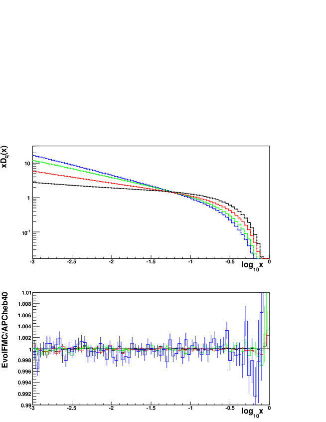
Figure 1: The upper plot shows the singlet quark distribution $xD_{q}(x,Q)$ evolved from $Q_{0}=1\,$GeV (black) to $Q=10$ (red), $100$ (green) and $1000$ (blue) GeV, obtained from EvolFMC (solid lines) and APCheb40 (dashed lines, hardly distinguishable), while the lower plot shows their ratio.

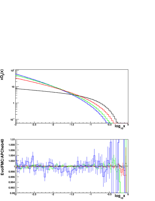
Figure 2: The upper plot shows the gluon distribution $xD_{q}(x,Q)$ evolved from $Q_{0}=1\,$GeV (black) to $Q=10$ (red), $100$ (green) and $1000$ (blue) GeV, obtained from EvolFMC (solid lines) and APCheb40 (dashed lines, hardly distinguishable), while the lower plot shows their ratio.

In Fig. 1 we show the resulting quark distributions obtained from the two programs (the upper plot) as well as their ratios (the lower plot). As one can see, these two calculations agree at the level of $0.2\%$, except for the $x$-region very close to $1$, where the MC statistics is low. The similar agreement has been found for the resulting gluon distributions, shown in Fig. 2. The precision of the presented results is limited by the statistical errors of the MC calculations.

4 One-loop CCFM equations of Kwieciński

The CCFM equations [12] describe the evolution of an unintegrated parton distributions $d_{K}(x,k^{T},Q)$ which depend on the parton transverse momentum $k^{T}$ in addition to the longitudinal momentum fraction $x$ and the scale $Q$. They are related to the integrated parton distribution of the DGLAP equations $D_{K}(x,Q)$ through the following relation

$$xD_{K}(x,Q)=\int d^{2}k^{T}\,xd(x,k^{T},Q)$$ (34)

Originally, the CCFM equations were derived for the unintegrated gluon distribution. In the all-loop approximation, they also take into account angular ordering (coherence) in the initial state gluon cascade for both large and small values of $x$. This leads to a new non-Sudakov form factor that sums virtual corrections for small $x$.

In the one-loop approximation, the angular ordering at small $x$ and the corresponding virtual corrections are subleading. Thus, the resulting equations contain only coherence in the real parton emissions for large $x$, including only the Sudakov form factor which resumes virtual corrections. At small $x$ the standard DGLAP transverse momentum ordering appears. The one-loop CCFM equations for both quark and gluon unintegrated distributions, written for the first time in [15], take the following form

$$xd_{K}(x,k^{T},Q) =xd^{0}_{K}(x,k^{T})$$

$$+\int\frac{d^{2}\vec{q}}{2\pi q^{2}}\theta(q-q_{0})\theta(Q-q)\int\limits_{x}^{1}\frac{dz}{z}\,z\mathcal{P}_{KJ}(q,z)\,\frac{x}{z}\,d_{J}\Bigl{(}\frac{x}{z},l^{T},q\Bigr{)},$$

$$\vec{l}^{T} =\vec{k}^{T}+(1-z)\vec{q}\,.$$ (35)

This equation is slightly more general than the original equation from Ref. [15] since it allows for the coupling constant (hidden in the splitting functions $\mathcal{P}_{KJ}(q,z)$) which depends both on $z$ and $q$. The iterative solution to eq. (35) reads

$$xd_{K} (x,k^{T},Q)=xd^{0}_{K}(x,k^{T})+\sum_{n=1}\int\limits_{0}^{1}dz_{0}\int d^{2}\vec{k}^{T}_{0}\sum_{K_{0},\ldots,K_{n-1}}$$

$$\Biggl{[}\prod_{i=1}^{n}\int\limits_{q_{0}}^{Q}\frac{d^{2}\vec{q_{i}}}{2\pi q_{i}^{2}}\,\theta(q_{i}-q_{i-1})\int\limits_{0}^{1}{dz_{i}}\,z_{i}\mathcal{P}_{K_{i}K_{i-1}}(q_{i},z_{i})\Biggr{]}xd^{0}_{K_{0}}\Bigl{(}z_{0},{k}^{T}_{0}\Bigr{)}$$

$$\delta\Bigl{(}x-\prod_{i=0}^{n}z_{i}\Bigr{)}\,\delta^{2}\Bigl{(}\vec{k}^{T}-\vec{k}^{T}_{0}+\sum_{i=1}^{n}(1-z_{i})\vec{q}_{i}\Bigr{)}\,,$$ (36)

where $K\equiv K_{n}$. As compared to the basic iterative solution of the DGLAP-type equation, eq. (2), the above series differs only by the presence of the independent angular integrals in $d^{2}q_{i}$ and by the presence of the delta function $\delta^{2}(\vec{k}^{T}-\dots)$, which in the Markovian-type algorithm plays only a “spectator” role. In addition, in eq. (36) the Sudakov form factor has not been explicitly worked out, as in eq. (2), and the initial condition $xd^{0}_{K}$ is now ${k^{T}}$-dependent. Having that in mind, we reorganize eq. (36) in the form similar to the DGLAP solution, eq. (2),

$$\begin{split}xd_{K}&(x,k^{T},t)=e^{-\Phi_{K}(t,t_{0})}xd^{0}_{K}(x,k^{T},t_{0})+\sum_{n=1}^{\infty}\;\int\limits_{0}^{1}dx_{0}\;\int d^{2}\vec{k}^{T}_{0}\sum_{K_{0},\ldots,K_{n-1}}\\ &\prod_{i=1}^{n}\bigg{[}\int\limits_{t_{0}}^{t}dt_{i}\;\Theta(t_{i}-t_{i-1})\int\frac{d\phi_{i}}{2\pi}\int\limits_{0}^{1}dz_{i}\bigg{]}e^{-\Phi_{K}(t,t_{n})}\prod_{i=1}^{n}\bigg{[}z_{i}\mathcal{P}_{K_{i}K_{i-1}}^{\Theta}(t_{i},z_{i})e^{-\Phi_{K_{i-1}}(t_{i},t_{i-1})}\bigg{]}\\ &~{}~{}~{}\times xd^{0}_{K_{0}}\Bigl{(}z_{0},{k}^{T}_{0},t_{0}\Bigr{)}\,\delta\big{(}x-x_{0}\prod_{i=1}^{n}z_{i}\big{)}\,\delta^{2}\Bigl{(}\vec{k}^{T}-\vec{k}^{T}_{0}+\sum_{i=1}^{n}(1-z_{i})\vec{q}_{i}\Bigr{)}\,,\end{split}$$ (37)

where as before $q_{i}=\exp(t_{i})$ and $\phi_{i}$ is the azimuthal angle of $\vec{q}_{i}$. Notice that $t=\ln Q$ plays now the role of the evolution variable.

It is now transparent that as described in Ref. [23] the forward Markovian algorithm EvolFMC can easily be extended to embed the generation of parton transverse momentum $k^{T}$. After $n$ steps of the forward Markovian evolution the transverse momentum of the off-shell parton entering the hard process becomes

$$\vec{k}^{T}_{n}=\vec{k}^{T}_{0}-\sum_{i=1}^{n}(1-z_{i})\vec{q}_{i}\,,$$ (38)

where $\vec{k}^{T}_{0}$ is an intrinsic parton transverse momentum and $\vec{q}_{i}$ a 2-dimensional evolution variable. The physical transverse momenta of emitted particles are

$$(1-z_{i})\vec{q}_{i}\,.$$ (39)

In the MC evolution $\vec{q}$ is constructed as follows:

$$\vec{q}_{i}=e^{t_{i}}\,(\cos\phi_{i},\sin\phi_{i}),$$ (40)

where $t_{i}$ is an evolution variable and $\phi_{i}$ is an azimuthal angle generated at each evolution step from a flat distribution in the range $[0,2\pi]$.

In our numerical tests, which will be reported in the next section, the intrinsic parton transverse momentum $k^{T}_{0}$ is generated at the initial evolution scale $t_{0}$ from the following $x$-independent distribution

$$\frac{1}{k_{0}^{2}}\,\exp\left\{\frac{-(k^{T}_{0})^{2}}{k_{0}^{2}}\right\},$$ (41)

where $k_{0}$ is some adjustable parameter, set to $1\,{\rm GeV}$ in our tests.

5 Numerical results for $k^{T}$-distributions

In the following we present results for the unintegrated parton distributions as functions of the transverse momentum $k^{T}$, generated by the forward Markovian MC program EvolFMC [32] according to the one-loop CCFM equation described in the previous section. The starting point of the evolution is $Q_{0}=1\,$GeV and the initial conditions are specified in eqs. (33) and (41).

In Figs. 3 and 4 we show the gluon distribution obtained from the CCFM equation with gluons only, as given by Marchesini and Webber in Ref. [13]. The distribution was additionally integrated over $x$. For rising values of the scale $Q$ such a gluon distribution moves towards large values of $k^{T}$, becoming at the same time less sensitive to the low $k^{T}$ region. This observation is summarized in Fig. 5 where we present the average gluon $(k^{T})^{2}$ as a function of $x$ for $Q=1,\,10,\,100$ and $1000\,$GeV.

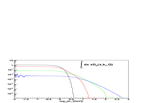
Figure 3: Gluon $k^{T}$ distributions integrated over $x$ for the one-loop CCFM equation of Marchesini–Webber, obtained from EvolFMC for Q = 1 (black), 10 (red), 100 (green) and 1000 (blue) GeV.

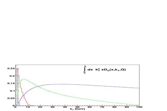
Figure 4: Gluon $k^{T}$ distributions multiplied by $(k^{T})^{2}$ integrated over $x$ for the one-loop CCFM equation of Marchesini–Webber, obtained from EvolFMC for Q = 1 (black), 10 (red), 100 (green) and 1000 (blue) GeV.

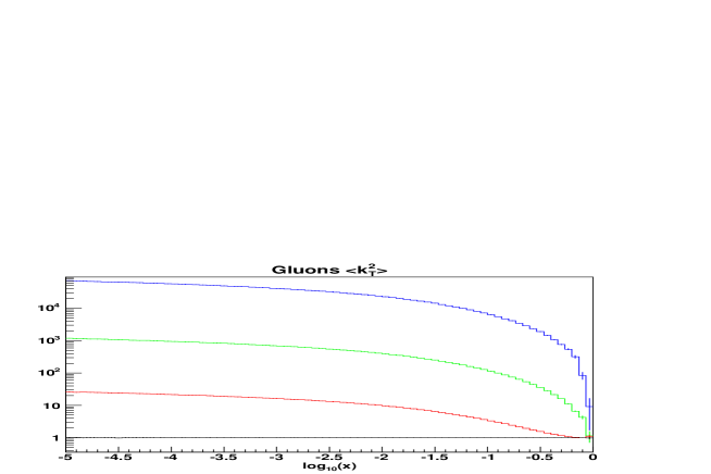
Figure 5: The average $(k^{T})^{2}$ of gluon as a function of $x$ for the one-loop CCFM equation of Marchesini–Webber, obtained from EvolFMC for Q = 1 (black), 10 (red), 100 (green) and 1000 (blue) GeV.

In Figs. 6 and 7, we show the results of the same studies for the full one-loop CCFM equation for the singlet quark and gluon distributions, given by Kwieciński et al. in Ref. [15]. The change of the distributions (integrated over $x$) with the hard scale $Q$ is the same as in the previous case. Both the quark and gluon distributions become less sensitive to the “soft” $k^{T}$ values moving towards the region of large $k^{T}$’s. This is also visible in Fig. 8 for the average transverse momentum for gluons and quarks. As expected, the average $k^{T}$ rises when $x\to 0$ [15].

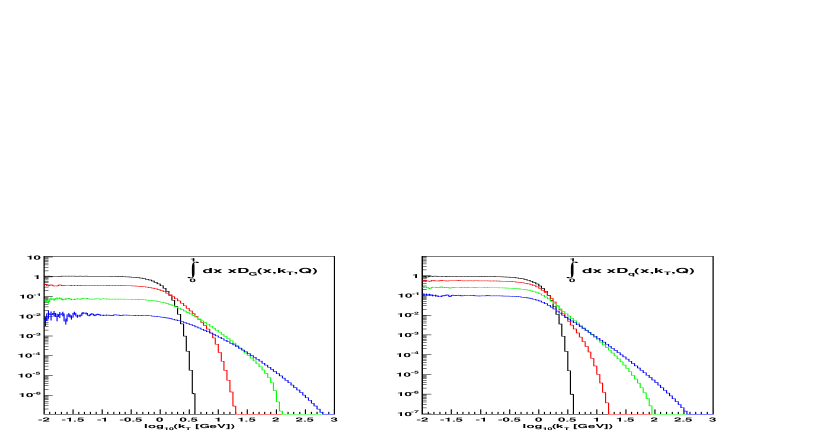
Figure 6: Gluons and quarks $k^{T}$ distributions integrated over $x$ for the one-loop CCFM equation of Kwieciński, obtained from EvolFMC for Q = 1 (black), 10 (red), 100 (green) and 1000 (blue) GeV.

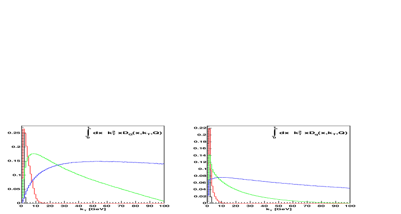
Figure 7: Gluons and quarks $k^{T}$ distributions multiplied by $(k^{T})^{2}$ integrated over $x$ for the one-loop CCFM equation of Kwieciński, obtained from EvolFMC for Q = 1 (black), 10 (red), 100 (green) and 1000 (blue) GeV.

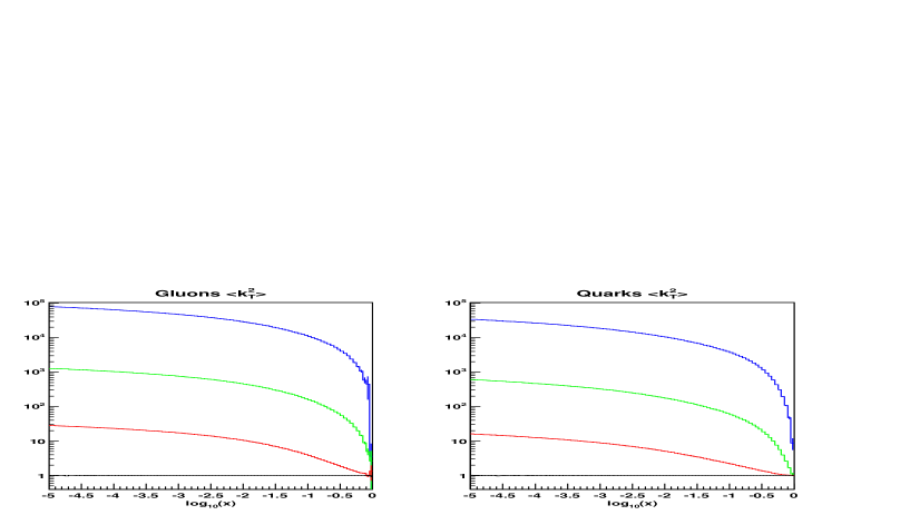
Figure 8: The average $(k^{T})^{2}$ of gluons and quarks as a function of $x$ for the one-loop CCFM equation of Kwieciński, obtained from EvolFMC for Q = 1 (black), 10 (red), 100 (green) and 1000 (blue) GeV.

6 Summary and outlook

In this work we have presented a systematic extension of the Monte Carlo algorithm that solves the DGLAP equation into the algorithm solving the one-loop CCFM equation. To this end two technical problems have been solved: the coupling constant has become $z$-dependent and the evolution in transverse momenta has been added, in addition to the evolution in the longitudinal momentum fractions $x$ in the parton distributions. The modification of the coupling constant has lead to the need of solving numerically the transcendental equation. First numerical results have been presented, confirming the known observations on CCFM unintegrated PDFs.

The presented algorithm for the one-loop CCFM evolution we consider as the first step in extending the other types of the QCD evolution equations available in our MC programs beyond that of the DGLAP type. In particular, implementing the complete CCFM evolution, both in the Markovian and non-Markovian (constrained) algorithms, see ref. [26], is now in an advanced stage. The presently implemented one-loop CCFM option will be used in the forthcoming studies of various aspects of the QCD evolution equations according to several different schemes.

Acknowledgments
We would like to thank Z. Wa̧s for the useful discussions. We thank for warm hospitality of the CERN PH Department were part of this work was done. The partial financial support of the MEiN research grant 1 P03B 028 28 (2005-08) is acknowledged.

References

• [1] L.N. Lipatov, Sov. J. Nucl. Phys. 20 (1975) 95;
V.N. Gribov and L.N. Lipatov, Sov. J. Nucl. Phys. 15 (1972) 438;
G. Altarelli and G. Parisi, Nucl. Phys. 126 (1977) 298;
Yu. L. Dokshitzer, Sov. Phys. JETP 46 (1977) 64.
• [2] E. G. Floratos, D. A. Ross, and C. T. Sachrajda, Nucl. Phys. B129, 66 (1977).
• [3] E. G. Floratos, D. A. Ross, and C. T. Sachrajda, Nucl. Phys. B152, 493 (1979).
• [4] G. Curci, W. Furmanski, and R. Petronzio, Nucl. Phys. B175, 27 (1980).
• [5] W. Furmanski and R. Petronzio, Phys. Lett. B97, 437 (1980).
• [6] S. Moch, J. A. M. Vermaseren, and A. Vogt, Nucl. Phys. B688, 101 (2004), hep-ph/0403192.
• [7] A. Vogt, S. Moch, and J. A. M. Vermaseren, Nucl. Phys. B691, 129 (2004), hep-ph/0404111.
• [8] L.N. Lipatov, Sov. J. Nucl. Phys. 23 (1976) 338;
E.A. Kuraev, L.N. Lipatov and V.S. Fadin, Sov. Phys. JETP 45 (1977) 199;
I.I. Balitsky and L.N. Lipatov, Sov. J. Nucl. Phys. 28 (1978) 822;
L.N. Lipatov, Sov. Phys. JETP 63 (1986) 904.
• [9] V.S. Fadin and L.N. Lipatov, Phys. Lett. B429 (1998) 127;
G. Camici and M. Ciafaloni, Phys. Lett. B412 (1997) 396 [Erratum-ibid. B417 (1998) 390]; Phys. Lett. B430 (1998) 349.
• [10] G. Altarelli, R. D. Ball, and S. Forte, Nucl. Phys. B742, 1 (2006), hep-ph/0512237.
• [11] M. Ciafaloni, D. Colferai, G. P. Salam, and A. M. Stasto, Phys. Lett. B635, 320 (2006), hep-ph/0601200.
• [12] M. Ciafaloni, Nucl. Phys. B296 (1988) 49;
S. Catani, F. Fiorani and G. Marchesini, Phys. Lett. B234 339, Nucl. Phys. B336 (1990) 18;
G. Marchesini, Nucl. Phys. B445 (1995) 49.
• [13] G. Marchesini and B. R. Webber, Nucl. Phys. B349, 617 (1991).
• [14] K. Golec-Biernat, L. Goerlich, and J. Turnau, Nucl. Phys. B527, 289 (1998), hep-ph/9712345.
• [15] J. Kwiecinski, Acta Phys. Polon. B33 (2002) 1809;
A. Gawron, J. Kwiecinski and W. Broniowski, Phys. Rev. D68 (2003) 054001;
A. Gawron, J. Kwiecinski, Phys. Rev. D70 (2004) 014003.
• [16] B. I. Ermolaev, M. Greco, and S. I. Troyan, Nucl. Phys. B594, 71 (2001), hep-ph/0009037.
• [17] S. Jadach and M. Skrzypek, Acta Phys. Polon. B35, 745 (2004), hep-ph/0312355.
• [18] S. Jadach and M. Skrzypek, Nucl. Phys. Proc. Suppl. 135, 338 (2004).
• [19] S. Jadach and M. Skrzypek, Acta Phys. Polon. B36, 2979 (2005), hep-ph/0504205.
• [20] S. Jadach and M. Skrzypek, Comput. Phys. Commun. 175, 511 (2006), hep-ph/0504263.
• [21] S. Jadach and M. Skrzypek, (2005), hep-ph/0509178, Report CERN-PH-TH/2005-146, IFJPAN-V-05-09, Contribution to the HERA–LHC Workshop, CERN–DESY, 2004–2005, http://www.desy.de/$\sim$heralhc/.
• [22] S. Jadach and M. Skrzypek, Nucl. Phys. Proc. Suppl. 157, 241 (2006).
• [23] K. Golec-Biernat, S. Jadach, W. Placzek, and M. Skrzypek, Acta Phys. Polon. B37, 1785 (2006), hep-ph/0603031.
• [24] S. Jadach, M. Skrzypek, and Z. Was, (2006), hep-ph/0701174.
• [25] P. Stokłosa and M. Skrzypek, Method of fitting PDFs for the Monte Carlo solutions of the evolution equations in QCD, report IFJPAN-IV-07-01, submitted to Acta Physica Polonica B.
• [26] S. Jadach, W. Płaczek, M. Skrzypek, P. Stephens, and Z. Wa̧s, Constrained MC for QCD evolution with rapidity ordering and minimum kT, 2007, hep-ph/0703281, Report FJPAN-IV-2007-3, CERN-PH-TH/2007-059.
• [27] D. Amati, A. Bassetto, M. Ciafaloni, G. Marchesini, and G. Veneziano, Nucl. Phys. B173, 429 (1980).
• [28] S. J. Brodsky, G. P. Lepage, and P. B. Mackenzie, Phys. Rev. D28, 228 (1983).
• [29] G. Sterman, Nucl. Phys. B281, 310 (1987).
• [30] H. Jung and G. P. Salam, Eur. Phys. J. C19, 351 (2001), hep-ph/0012143.
• [31] S. Jadach, Comput. Phys. Commun. 152, 55 (2003), physics/0203033.
• [32] S. Jadach et al., The Markovian Monte Carlo program EvolFMC for the forward QCD evolution, unpublished, 2006, the C$++$ code.
• [33] K. Golec-Biernat, APCheb40, the Fortran code available on the request from the author, unpublished.