Measuring $\gamma$ with $B^{0}\rightarrow D^{0}K^{*0}$ at BaBar

Abstract

We present a feasibility study for a new analysis for extracting the angle $\gamma$ of the Unitarity Triangle from the study of the neutral B meson decays. We reconstruct the decay channel $B^{0}\rightarrow\bar{D^{0}}K^{*0}$ with the $K^{*0}\rightarrow K^{+}\pi^{-}$ and the $\bar{D}^{0}\rightarrow K_{S}\pi^{+}\pi^{-}$ using a $D^{0}$ Dalitz analysis technique. The sensitivity to the angle $\gamma$ comes from the interference of the $b\rightarrow c$ and $b\rightarrow u$ processes contributing to the same final state and by the fact that the $B^{0}(\bar{B^{0}})$ can be unambiguosly identified through the sign of electric charge of the kaon from $K^{*0}(\bar{K^{*0}})$ decay. The impact of the result of such analysis is evaluated for the actual BaBar statistics.

I The technique

Various methods related to $B^{-}\to D^{(*)0}K^{(*)-}$ decays have been proposed to determine the UT angle $\gamma$. Within them, the one that gives the best error on $\gamma$ is the Dalitz method DalitzBaBar DalitzBelle .

We propose to measure the angle $\gamma$ using a Dalitz analysis applied to neutral B mesons. In general, since the neutral B mesons mix, interference effects between $b\to c$ and $b\to u$ decay amplitudes in $B^{0}$ decays (for instance into $D^{(*)\pm}\pi^{\mp}$ final states) are studied for the determination of the combination of UT angles $2\beta+\gamma$. In this case the tagging technique and a time dependent analysis are required. This can be avoided if the final states contain a particle which allows to unambiguously identify if a $B^{0}$ or $\bar{B}^{0}$ has decayed. This is the case of neutral B mesons decaying into $\bar{D}^{0}[K^{+}\pi^{-}]$ final states, where the flavor of the B meson can be determined through the sign of the electric charge of the Kaon.

One of the relevant parameter in those kind of analysis is the ratio between the $b\to u$ and $b\to c$ amplitudes, which can be expressed by :

$$r_{B}(D^{0}K^{*0})=\frac{|{\cal A}({D}^{0}{K}^{*0})|}{|{\cal A}(\bar{D^{0}}{K}^{*0})|}=\frac{|V_{ub}|}{\lambda|V_{cb}|}\frac{{\cal A_{\rm{strong}}}({D}^{0}{K}^{*0})}{{\cal A_{\rm{strong}}}(\bar{D^{0}}{K}^{*0})}.$$ (1)

The sensitivity to $\gamma$ is proportional to the $r_{B}$ value. Considering the CKM factors in the $b\to c$ and $b\to u$ transitions and the fact that in both cases the processes are mediated by a color suppressed diagram, we expect $r_{B}(D^{0}K^{*0})$ to be in the range [0.3-0.5], larger than for the equivalent ratio in the charged B sector, which has been found to be of the order 0.1 Bona:2005vz .

II Structure of the analysis

In the analysis on data we would perform an unbinned maximum likelihood fit in order to extract the interesting quantities: the likelihood will contain a product of a yields pdf and a CP pdf (only the latter has, within its variables, the weak phase $\gamma$).

In our feasibility study, we assume the yields pdf to be a function of the classic BaBar analysis variable $m_{ES}$ and of a variable that is able to discriminate between $B\bar{B}$ and continuum events ($q\bar{q}$ events, with $q=u,d,s,c$). For the distributions of those variables we make some realistic assumptions inspired by BaBar analysis.

In writing the CP pdf, we have an additional difficulty, with respect to the $B^{-}\rightarrow D^{0}K^{-}$ Dalitz analysis. This is due to the fact that the natural width of the $K^{*0}$ is not small ($\sim$50 MeV) and hence the interference with the other $B^{0}\to\bar{D^{0}}(K\pi)_{\rm{non-}K^{*}}^{0}$ processes may not be negligible. We follow the formalism introduced in gronau2002 and also used in the $B^{-}\rightarrow D^{0}K^{*-}$ BaBar analysis in order to solve this problem.

We introduce the effective quantities $r_{S}$, $k$ and $\delta_{S}$ defined as :

$$r_{s}^{2}=\frac{\Gamma(\bar{B^{0}}\to\bar{D^{0}}(K^{+}\pi^{-}))}{\Gamma(\bar{B^{0}}\to D^{0}(K^{+}\pi^{-}))}=\frac{\int dp\ |A_{up}^{2}|}{\int dp\ |A_{cp}^{2}|}$$ (2)

$$ke^{i\delta_{S}}=\frac{\int dp\ A_{cp}A_{up}e^{i\delta_{p}}}{\sqrt{\int dp\ |A_{cp}^{2}|\ \int dp\ |A_{up}^{2}|}}\,,$$ (3)

where $0\leq k\leq 1$ for the Schwartz inequality and $\delta_{S}\in[0,2\pi]$. In the limit of a $B\to$2-body decay, such as $\bar{B^{0}}\to D\bar{K^{0}}$ we have : $r_{S}\rightarrow r_{B}$, $\delta_{S}\rightarrow\delta_{B}$ (the phase difference between the $V_{ub}$ and the $V_{cb}$ amplitudes of Eq.1) and k=1. $A_{cp}$, $A_{up}$ are real and positive. The subscript $c$ and $u$ refer to the $b\to c$ and $b\to u$ transitions, respectively. The index $p$ indicates the position in the phase space of $D^{0}K^{+}\pi^{-}$.

Applying this formalism, we write the CP pdf as follows:

$$\Gamma(\bar{B^{0}}(B^{0})\to D[\to K^{0}_{S}\pi^{-}\pi^{+}]K^{-}\pi^{+}(K^{+}\pi^{-}))\propto$$

$$|f_{\mp}|^{2}+r_{s}^{2}|f_{\pm}|^{2}+2kr_{s}|f_{\mp}||f_{\pm}|\cos(\delta_{S}+\delta_{D}(m_{\mp}^{2},m_{\pm}^{2})\mp\gamma)\,,$$ (4)

where $\delta_{D}(m_{\mp}^{2},m_{\pm}^{2})$ is the strong phase difference between $f(m_{\pm}^{2},m_{\mp}^{2})$ and $f(m_{\mp}^{2},m_{\pm}^{2})$ and $r_{s}$, $k$ and $\delta_{S}$ are defined in Eqs. (2) and (3). We have simplified the notation using $f_{\pm}\equiv f(m_{\pm}^{2},m_{\mp}^{2})$ and $f_{\mp}\equiv f(m_{\mp}^{2},m_{\pm}^{2})$.

The Dalitz structure of the decay $D^{0}\rightarrow K_{S}\pi\pi$ is well known and it has already been used in Dalitz analysis in the charged B sector DalitzBaBar DalitzBelle .

III the $k$ and $r_{S}$ parameters

We performe a study to evaluate the possible variation of $r_{S}$ and $k$ on the B Dalitz plot. For this purpose we use a B Dalitz model as suggested by the recent measurements ref:polci , ref:cavoto . The model assumed for the decay parametrizes the amplitude $A$ at each point $k$ of the Dalitz plot as a sum of two-body decay matrix elements and a non-resonant term according to the following expression :

$$A_{c_{k}(u_{k})}e^{i\delta_{c_{k}(u_{k})}}=\sum_{j}a_{j}e^{i\delta_{j}}BW^{j}_{k}(m,\Gamma,s)+a_{nr}e^{i\phi_{nr}}$$ (5)

We consider a region within $\pm$ 48 MeV from the nominal mass of the $K^{*0}$(892) resonance and we obtain the distribution of $r_{S}$, $k$ and $k\times r_{S}$ by randomly varying all the strong phases between [0-2$\pi$] and the amplitudes up to $\pm 30\%$ of their nominal value (shown in table 1). Only for the $D_{s,2}(2573)^{\pm}$ resonance, the variation is up to $\pm 200\%$ of its nominal value.

	$M(GeV/c^{2})$	$W(GeV/c^{2})$	$J^{P}$	$a(V_{cb})$	$a(V_{ub})$
$D_{s,2}(2573)^{\pm}$	2.572	0.015	$2^{+}$	0	0.02
$D_{2}^{*}(2460)^{\pm}$	2.459	0.029	$2^{+}$	1.0	0
$D_{0}^{*}(2308)^{\pm}$	2.403	0.283	$0^{+}$	1.0	0
$D_{0}^{*}(2010)^{\pm}$	2.0100	0.000096	$1^{-}$	-	-
$K^{*}(892)^{0}$	0.89610	0.0507	$1^{-}$	1.0	0.4
$K_{0}^{*}(1430)^{0}$	1.412	0.294	$0^{+}$	0.3	0.12
$K_{2}^{*}(1430)^{0}$	1.4324	0.109	$2^{+}$	0.15	0.06
$K^{*}(1680)^{0}$	1.717	0.322	$1^{-}$	0.2	0.08
Non resonant	-	-	-	-	-

Table 1: List of mass ($M$), widths ($W$) and quantum numbers of the resonances considered in our model. The last two columns present the chosen values of the coefficients $a_{j}$ for the $V_{cb}$ and $V_{ub}$ transitions respectively. Note that the phase $\delta_{j}$ are not indicated and their choice is arbitrary.

The distribution we obtain for $r_{S}$ and $k$ are shown in figure 1;

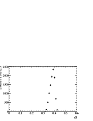
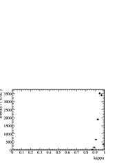
Figure 1: Distribution of $r_{S}$ and $k$ in a region within $\pm$ 50 MeV the nominal mass of the $K^{*0}$(892) resonance ($m_{K\pi}$ in the range [0.7159-0.8951] $GeV^{2}$). This distribution has been obtained by randomly varying all the strong phases (between [0-2$\pi$]), the amplitudes (between [0.7-1.3] of their nominal value (except those relative to $K^{*}$ which has been fixed to 0.4 and for the $V_{ub}$ amplitude of the $D_{s,2}(2573)^{\pm}$ which has been varied between [0.-2.] of its nominal value) given in Table 1).

The results is that, in $K^{*0}$(892) mass region, $r_{S}$ can vary between 0.3 and 0.45 depending upon the values of the phases and of the amplitudes contributing in the $K^{*0}$ region. In absence of pollution we would have expected $r_{S}=r_{B}=0.4$. The distribution of $k$ is quite narrow, centered to 0.95 with an error of 0.03.

For this reason the value of $k$ can be fixed to 0.95 and the effect of its variation (within a reasonable interval) will be considered a systematic error.

IV CP fit studies

We perform an intensive toy-MC study on the CP fit, assuming the actual BaBar statistics ($350\mbox{fb}^{-1}$). We assume to have $35$ signal events, about $2000$ continuum background events and $250$ $B\bar{B}$ background events.

IV.1 Polar coordinates

We first perform toy-MC studies in polar coordinates. In figure 2 we observe the known linearity problem: due to the dependence of the likelihood on $r_{S}$, we tend to get from the fit a value of $r_{S}$ higher than the true (generated) one and consequently to underestimate the error on $\gamma$.

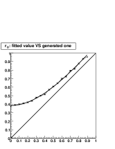
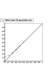
Figure 2: Distribution of $r_{S}^{FIT}$ vs $r_{S}^{GEN}$ from toy MC for different generated values.The toy-MC have been generated assuming $350\mbox{fb}^{-1}$(left plot) and 10 times the statistics (right plot).

It is evident that the linearity effect (still visible in the results of the tests at high statistics) is not the only problem that affects our measurement. In fact, as it can be seen from the left plot, also for high values of $r_{S}^{GEN}$ the results for $r_{S}^{fit}$ vs $r_{S}^{GEN}$ do not tend to the curve $r_{S}^{fit}=r_{S}^{GEN}$ (the black curve in the plots). We thus conclude that we cannot fit in polar coordinates (with $r_{S}$, $\gamma$ and $\delta_{S}$ floating) because of the two effects: the linearity and the low statistics and that is the second one that dominates (at least for $r_{S}\approx 0.4$, as it is expected to be for our measurement).

IV.2 Cartesian coordinates

We then perform a toy-MC study in cartesian coordinates ref:cart . The use of these coordinates normally solves the linearity problem (DalitzBaBar , DalitzBelle ).

From the toy-MC the four variables appear to be biased and show a non-Gaussian behaviour. In table 2, we summarize the results of toy-MC where we generated for the yields the values we expect on $350fb^{-1}$ (left column) and the results of toy-MC for 10 times the now available BaBar statistics (right column). As it can be seen in the left column, all the variables are biased and the $\sigma$ of their pulls are not compatibles with $1$. This effect disappears at high statistics. We conclude that, with the now available statistics, we cannot perform the measurement in cartesian coordinates.

-	$now$	$10x$ stat
$\mu^{PULL}_{x_{+}}$	$-0.52\pm 0.05$	$-0.04\pm 0.05$
$\sigma^{PULL}_{x_{+}}$	$0.82\pm 0.03$	$0.97\pm 0.04$
$\mu^{PULL}_{x_{-}}$	$-0.07\pm 0.05$	$-0.02\pm 0.05$
$\sigma^{PULL}_{x_{-}}$	$0.78\pm 0.04$	$0.99\pm 0.04$
$\mu^{PULL}_{y_{+}}$	$-0.18\pm 0.05$	$-0.05\pm 0.06$
$\sigma^{PULL}_{y_{+}}$	$0.79\pm 0.04$	$1.01\pm 0.04$
$\mu^{PULL}_{y_{-}}$	$0.40\pm 0.05$	$-0.03\pm 0.05$
$\sigma^{PULL}_{y_{-}}$	$0.79\pm 0.04$	$1.03\pm 0.04$

Table 2: Pull distributions for cartesian coordinates on 500 toy-MC with a signal background configuration similar to the one we find on data (left column) and for 10 times the statistics (right column).

IV.3 Measurement strategy

We conclude that, with the now available BaBar statistics, the measurement strategy would be extracting from the fit $\gamma$ as a scan with respect to $r_{B}$ (i.e. by performing a likelihood scan on $\gamma$ for each value of $r_{B}$ with $\gamma$, $\delta$ and all the yields parameters floated in the fit).

In this way we would extract from data the maximum possible information for the available statistics: an information on $\gamma$ and not on $r_{B}$. The $\gamma$ distribution obtained in that way, already very interesting on its own, would be very precious when combined with an experimental input for $r_{B}$. The coverage tests on toy-MC generated with different values of $r_{S}$ show that we have no bias in this fit configuration.

V impact of the measurement

In this section we show, on one chosen toy-MC, what would be the impact of a real mesurement. In figure 3 we show the output of our fit: a likelihood scan of $\gamma$ with respect to $r_{S}$.

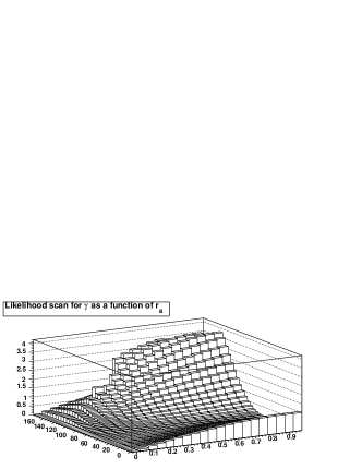
Figure 3: Negative Log Likelihood scan for $\gamma$ for different values of $r_{B}$. The distribution is obtained on a chosen toy-MC.

This distribution, when combined with a fake $r_{S}$ measurement ($r_{S}=0.35\pm 0.15$) gives $\gamma$ with an error of $46^{o}$. A measurement of $r_{S}$ with such an error is what we could expect to obtain, if $r_{S}=0.35$, on $500\mbox{fb}^{-1}$ data from an analysis of $B^{0}\rightarrow D^{0}K^{*0}$ with the $D^{0}$ in flavor modes.

Clearly, this is just a example on a chosen toy-MC and it is not necessarily representative of what we will find on data. Indeed we found, on toy-MC studies, that in a small percentage of cases we can be much less sensitive to $\gamma$. That problem has been found to depend on the low number of signal events (such that in some cases those events happen to be in poorly sensitive regions of the $D^{0}$ Dalitz plot) and it will therefore disappear with the increasing of the statistics. Still, our test shows that we could have a result on $\gamma$ that is competitive with the charged B Dalitz analysis (the analysis made on BaBar data gives today an error on $\gamma$ of $42^{o}$).

References

- (1) B. Aubert et al. [BABAR Collaboration], arXiv:hep-ex/0607104.
- (2) A. Poluektov et al. [Belle Collaboration], Phys. Rev. D 73, 112009 (2006) [arXiv:hep-ex/0604054].
- (3) M. Bona et al. [UTfit Collaboration], JHEP 0507, 028 (2005) [arXiv:hep-ph/0501199]. Updated results available at http://www.utfit.org/
- (4) M. Gronau, Phys. Lett. B557, 198-206 (2003).
- (5) F. Polci, M.-H. Schune and A. Stocchi [arXiv:hep-ph/0605129].
- (6) G.Cavoto et al., Proceedings of the CKM 2005 Workshop (WG5), UC San Diego, 15-18 March 2005, hep-ph/0603019.
-
(7)
The parameterization given in Eq. (4) can be rewritten in terms of the
cartesian coordinates and
as