Abstract

We discuss the physics case of a high luminosity $B$-Factory running at the $\Upsilon(5S)$ resonance. We show that the coherence of the $B$ meson pairs is preserved at this resonance, and that $B_{s}$ can be well distinguished from $B_{d}$ and charged $B$ mesons. These facts allow to cover the physics program of a traditional $B$-Factory and, at the same time, to perform complementary measurements which are not accessible at the $\Upsilon(4S)$. In particular we show how, despite the experimental limitations in performing time-dependent measurements of $B_{s}$ decays, the same experimental information can be extracted, in several cases, from the determination of time-integrated observables. In addition, a few examples of the potentiality in measuring rare $B_{s}$ decays are given. Finally, we discuss how the study of $B_{s}$ meson will improve the constraints on New Physics parameters in the $B_{s}$ sector, in the context of the generalized Unitarity Triangle analysis.

1 Introduction

The study of $B$ mesons at the $B$-Factories has considerably improved our understanding of flavour physics in the Standard Model (SM), confirming that CP violation is well described by the Cabibbo-Kobayashi-Maskawa (CKM) matrix [1]. In particular, the agreement between the measured value of $\sin 2\beta$ in $b\rightarrow c\bar{c}s$ decays [2, 4] and the prediction from the indirect constraints on the CKM parameters $\bar{\rho}$ and $\bar{\eta}$ [3] can be considered the first precision test of the CKM mechanism. Additional constraints have been added, leading to a remarkable improvement of the determination of the parameters of the CKM matrix [5].

A large set of these measurements is based on the study of the coherent $B$–$\bar{B}$ state, produced by the decay of the $\Upsilon(4S)$. The possibility of studying simultaneously time-dependent CP asymmetries and rates in several $B$ decays to charged and neutral particles pushed the physics program of BaBar [6] and Belle [7] well beyond the initial expectations. The key ingredients of the success of BaBar and Belle are the large achieved luminosities and the clean environment in which $B$ mesons are reconstructed. The two collaborations are expected to improve the situation by doubling their datasets in the next two years.

Recently, the study of $B$ physics received an additional boost by the results from the Tevatron experiments CDF [8] and D$\O$ [9]. In particular, the measurement of the oscillation frequency of the $B_{s}$–$\bar{B}_{s}$ system, $\Delta m_{s}$ [10] and the comparison to the prediction from the indirect determination [4] represents an additional test of the SM, having a value comparable to the measurement of $\sin 2\beta$. In the next future, new measurements will be added, thanks to the increased dataset of the Tevatron experiments and the start of the LHCb program [11].

Since these measurements will be performed at hadronic machines, where $B_{d}$, $B_{u}$, $B_{s}$ and $B_{c}$ mesons are simultaneously produced, it will be possible to cover a much larger physics sample. In particular, from the study of $B_{s}$ mesons it is possible to extract some of the fundamental quantities that are also accessible at the $B$-Factories (as the CKM phase $\gamma$ or New Physics (NP) parameters) with reduced theoretical uncertainty with respect to the case of $B_{d}$ mesons. In addition, thanks to the different quark content of the initial state, several $B_{s}$ decays, which are comparable to interesting decay modes of the $B_{d}$ meson, can provide more experimental information. For instance, the decay $B_{s}\rightarrow KK$ has the same interesting features of $B_{d}\rightarrow K\pi$, but since it is a CP eigenstate, a study of the time-dependent CP asymmetry can be performed. Another example is $B_{s}\rightarrow J/\psi\phi$, similar to $B_{d}\rightarrow J/\psi K^{*0}$, but which can be reconstructed in a CP eigenstate with all charged particles in the final state and therefore with a higher efficiency. 

However, we stress that in these latter cases the measurements will be performed in a very different context with respect to the clean $e^{+}e^{-}$ environment. Because of this, several measurements that can be accessed at the $B$-Factories, such as those involving neutral particles (i.e. $\pi^{0}$’s, $\eta^{\prime}$ decays, radiative photons, etc.) can not be carried out with the same high accuracy as in an $e^{+}e^{-}$ facility. We thus suggest here to investigate the possibility of performing them at an $e^{+}e^{-}$ environment. Such opportunity might be provided by a next generation $B$-Factory, running also at the $\Upsilon(5S)$ resonance [13]. We will show how a run at the $\Upsilon(5S)$ could provide, with respect to already approved experiments, both complementary informations and independent determinations of interesting CKM parameters and quantities sensitive to NP.

In the recent past, CLEO and Belle performed short runs at the $\Upsilon(5S)$, measuring the main features of this resonance with a few collected data. These first results give just a flavour of the potentiality of a $B$-Factory running at the $\Upsilon(5S)$, which is the subject of this paper.

We assume the same detector performances of the existing $B$-Factory experiments and we use a full detector simulation to study the physics potential of running at $\Upsilon(5S)$, as a function of the integrated luminosity.

We show that it is possible to separate $B_{s}$ mesons from $B_{d}$ and charged $B$ mesons, even in presence of several photons in the final state. In this way, running at the $\Upsilon(5S)$, it would be possible to perform the same physics measurements than at the present $B$-Factories, after imposing kinematic cuts to reject $B_{s}$ events.

2 The $\Upsilon(5S)$ Production and Decays

The $\Upsilon(5S)$ resonance is a $J^{CP}=1^{--}$ state of a $b\bar{b}$ quark pair, having an invariant mass $m_{\Upsilon(5S)}=(10.865\pm 0.0008)$ GeV [14]. The cross section of $\Upsilon(5S)$ production in $e^{+}e^{-}$ collisions is $\sigma(e^{+}e^{-}\rightarrow\Upsilon(5S))=0.301\pm 0.002\pm 0.039$ nb [15]. This resonance was discovered by CLEO at the CESR $e^{+}e^{-}$ collider, measuring the total cross section above the $\Upsilon(4S)$ resonance [16]. The distribution of $R=\sigma(e^{+}e^{-}\rightarrow q\bar{q})/\sigma(e^{+}e^{-}\rightarrow\mu\mu)$ as a function of the invariant mass is shown in Fig. 1.

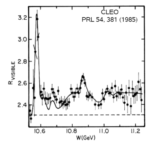
Figure 1: CLEO measurement of $R=\sigma(e^{+}e^{-}\rightarrow q\bar{q})/\sigma(e^{+}e^{-}\rightarrow\mu\mu)$ as a function of the invariant mass $W$, in the region of $W$ $\sim 11$ GeV [16].

The knowledge on the properties of this bound state comes from the $0.42$ fb^-1 collected by the CLEO experiment at CESR [16] and by the $1.86$ fb^-1 collected by the Belle detector at KEKB, during the $\Upsilon(5S)$ engineering run [17]. The Belle collaboration has also collected a sample of about $20$ fb^-1 during June 2006.

Unlike the $\Upsilon(4S)$ state, this resonance is heavy enough to decay in several $B$ meson states. In particular, it can decay to vector-vector (VV), pseudoscalar-vector (PV), and pseudoscalar-pseudoscalar (PP) combinations of $B^{(*)\pm}$, $B_{d}^{(*)}$ and $B_{s}^{(*)}$ mesons. The $\Upsilon(5S)$ resonance can also decay into $B^{(\ast)}\bar{B}^{(\ast)}\pi$.

In the case of PP decays, the two $B$ mesons are produced in a $1^{--}$ state, as in the case of the $\Upsilon(4S)$ resonance. When the produced mesons are neutral, they exhibit flavour oscillations, because of the coherence of the initial state, the oscillation frequency being determined by the mass differences $\Delta m_{d,s}$.

The case of PV and VV decay is more complicated. The vector states $B_{q}^{\ast}$ ($q=u,d,s$) decay in $B_{q}^{\ast}\rightarrow B_{q}\gamma$ through an electromagnetic interaction which, up to a very good level of approximation, can be considered as an instantaneous process. Under this assumption, it can be shown (see Sec. 4.1) that the time evolution of VV states is similar to that of the PP state. For events generated by PV decays, a difference comes from the opposite eigenvalue of the charge-conjugation operator.

Quark models [18] predict the production to be mainly in the excited final states $B_{d,s}^{\ast}\bar{B_{d,s}^{\ast}}$ with $B_{d,s}^{\ast}\rightarrow B_{d,s}\gamma$. Even if relative branching ratios (BR) of $\Upsilon(5S)$ are not precisely known yet, the current measurements confirm this picture. We summarize in Tab. 1 the corresponding experimental results, as reported by CLEO [15] and BELLE [17], along with the values used in this paper. For unmeasured values, we made educated guesses based on the predicted (and observed) VV dominance.

$\Upsilon(5S)$ Decay Modes	CLEO	BELLE	This Paper
$B_{s}^{(*)}\bar{B}_{s}^{(*)}$ $\left[\%\right]$	$26^{+7}_{-4}$	$21^{+6}_{-3}$	26
$(B_{s}^{*}\bar{B}_{s}^{*})/(B_{s}^{(*)}\bar{B}_{s}^{(*)})$	$-$	$0.94^{+0.06}_{-0.09}$	0.94
$(B_{s}^{*}\bar{B}_{s}+B_{s}\bar{B}_{s}^{*})/(B_{s}^{(*)}\bar{B}_{s}^{(*)})$	$-$	$-$	0.06
$(B_{s}\bar{B}_{s})/(B_{s}^{(*)}\bar{B}_{s}^{(*)})$	$-$	$-$	$-$
$B_{d,u}^{*}\bar{B}_{d,u}^{*}$ $\left[\%\right]$	$43.6\pm 8.3\pm 7.2$	$-$	44
$B_{d,u}\bar{B}_{d,u}^{*}+B_{d,u}^{*}\bar{B}_{d,u}$ $\left[\%\right]$	$14.3\pm 5.3\pm 2.7$	$-$	14
$B_{d,u}\bar{B}_{d,u}$ $\left[\%\right]$	$<13.8$	$-$	-
$B_{d,u}\bar{B}_{d,u}^{(*)}\pi+B_{d,u}^{(*)}\bar{B}_{d,u}\pi$ $\left[\%\right]$	$<19.7$	$-$	16
$B_{d,u}\bar{B}_{d,u}\pi\pi$ $\left[\%\right]$	$<8.9$	$-$	-

Table 1: BR of $\Upsilon(5S)$ decays, measured by CLEO [15] and BELLE [17] collaborations. The last column shows the values used throughout this paper.

The numbers quoted in the table, together with the different values of the cross sections, show that $B_{d}$ and charged $B$ mesons can be produced at the $\Upsilon(5S)$, with a rate about six times smaller than at the $\Upsilon(4S)$. This fact should be kept in mind: a reduction in the statistics of $B_{d}$ and charged $B$ mesons is the price to pay in order to study $B_{s}$ particles at a $B$-Factory.

3 Reconstruction of $B$–$\bar{B}$ pairs

The reconstruction of $B$–$\bar{B}$ pairs at the $\Upsilon(5S)$ proceeds like at the traditional $B$-Factories. The only relevant difference is the fact that several final states can be produced, with different momenta.

In the case of $B_{s}$ mesons, the largest fraction ($\sim 94\%$ of the events) is produced in a VV mode. One can then tune the event reconstruction and selection on these events, considering the PV and the PP modes as a source of background. To avoid decreasing the reconstruction efficiency, one should not look for either the photons produced by the $B_{s,d}^{*}$ decay or the one or more pions produced in the continuum $b\bar{b}$ production.

At a traditional $B$-Factory, $B\bar{B}$ events are distinguished from $q\bar{q}$ background ($q=u,d,s,c$) using a set of variables related to the distribution of the decay products in the center-of-mass (CM) system of the $\Upsilon$ resonance. We consider here the two quantities $L_{0}$ and $L_{2}$, defined as [19]

$$L_{j}\equiv\sum_{i}|{\bf p}^{*}_{i}||\cos\theta^{*}_{i}|^{j}~{}(j=0,2),$$ (1)

where ${\bf p}^{*}_{i}$ is the momentum of particle $i$ in the $e^{+}e^{-}$ rest frame, $\theta^{*}_{i}$ is the angle between ${\bf p}^{*}_{i}$ and the thrust axis of the $B$ candidate and the sum runs over all reconstructed particles except for the $B$-candidate daughters. In data analyses, $L_{0}$ and $L_{2}$ are typically combined into a Fisher discriminant ${\mathcal{F}}$ [20]. Alternatively, the ratio $L_{2}/L_{0}$ is used [21]. The discriminating power against the $q\bar{q}$ background for these two variables is very close, so that we use one or the other in the subsequent sections.

At the $\Upsilon(5S)$, $L_{0}$ and $L_{2}$ preserve all their features, even in presence of additional unreconstructed particles (photons and pions) produced with the $B\bar{B}$ pair. This is shown in Fig. 2, where the distribution of the ratio $L_{2}/L_{0}$ for $B_{s}\rightarrow J/\psi\phi$ generated events is given for PP(continuous line) and VV (dots) events. We do not distinguish between VV, PV, and PP in the following, when dealing with topological variables.

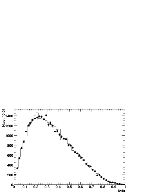
Figure 2: Distribution of $L_{2}/L_{0}$ for $B_{s}\rightarrow J/\psi\phi$ events simulated at the $\Upsilon(5S)$ resonance in a VV (dots) and PP (black line) configurations.

Kinematic variables are also used to reject background. At the $\Upsilon(4S)$, a $B\bar{B}$ event is usually characterized by the two following variables:

• $\Delta E=E_{B}^{\ast}-\sqrt{s}/2$, the energy difference between the reconstructed $B$ candidate in the center of mass (CM) frame $E_{B}^{\ast}$ and one half the total CM energy $\sqrt{s}$.

• the beam-energy substituted mass $m_{ES}=\sqrt{(s/2+{\mathbf{p}}_{i}\cdot{\mathbf{p_{B}}})^{2}/E_{i}^{2}-{\mathbf{p_{B}}}^{2}}$, where the $B$ momentum ${\mathbf{p_{B}}}$ and the four-momentum $(E_{i},{\mathbf{p_{i}}})$ of the $e^{+}e^{-}$ initial state are defined in the laboratory frame.

These two variables are found to be Gaussian distributed and almost uncorrelated for those $B$ decays having only charged tracks in the final state. For $B$ mesons coming from $\Upsilon(4S)$ decays, $m_{ES}$ ($\Delta E$) peaks at the value of the $B_{d}$ mass (at zero). The presence of photons in the final state (coming from decays of intermediate particles, radiative $B$ decay or bremsstrahlung) introduces a correlation (typically less than $20\%$), induced by the missing energy. In these cases, it was found [21] that a better signal identification is achieved replacing $m_{ES}$ with $m_{miss}$, defined as $m_{miss}=|p_{e^{+}e^{-}}-\tilde{p}_{B}|$, where $p_{e^{+}e^{-}}$ is the four-momentum of the $e^{+}e^{-}$ initial state and $\tilde{p}_{B}$ is the four-momentum of the $B$ candidate after applying a mass constraint on it.

To illustrate the kinematic properties of $B$ mesons coming from $\Upsilon(5S)$ decays, we consider the case of $\Upsilon(5S)\rightarrow B_{s}^{*}B_{s}^{*}$ events. After the two $B_{s}^{*}\rightarrow B_{s}\gamma$ decays, the final state is represented by the decay products of the two $B_{s}$ mesons and by the two additional photons which are not reconstructed. When calculating $\Delta E$ from the observed decay products, $E_{B}^{\ast}$ assumes the value of the energy of the $B_{s}$ meson, while the value to use for $\sqrt{s}/2$ corresponds to half the energy of the $B_{s}^{*}B_{s}^{*}$ system. This difference generates a shift of the $\Delta E$ distribution of $-47$ MeV, corresponding to the mass difference $m_{B_{s}}-m_{B^{*}_{s}}$. In addition, the $B_{s}$ momentum distribution is smeared by the spread of the photon energy in the CM frame, since the photon is monochromatic only in the $B_{s}^{*}$ rest frame, while the laboratory frame is boosted  and the energy of the photon becomes a function of the polar angle in the CM frame. At the same time, $m_{ES}$ values are shifted by the same quantity to larger values. This is shown in Fig. 3, where the distribution of $B_{d,s}\rightarrow J/\psi\phi$ events in the $\Delta E$ vs $m_{ES}$ plane is given. For $B_{s}$ decays the three bumps (corresponding to PP, PV and VV decays) are aligned along a straight line, identified by the relation: $\Delta E=-(m_{ES}-m_{B_{s}})$. Similar considerations are valid for $B_{d}$ and charged $B$ mesons.

For $m_{miss}$ the situation is more complicated, since the calculation of this variable requires a mass hypothesis for the reconstructed $B$ ($B_{d}$ or $B_{s}$ meson). One is forced to define two variables, $m_{miss}^{d}$ and $m_{miss}^{s}$, and to use one or the other according to the case under study.

In the following, we present three examples of $B$ decays at the $\Upsilon(5S)$ resonance. We start from the simple case of a final state without neutral particles ($B_{d,s}\rightarrow J/\psi\phi$). After showing the good performances in separating VV events from PV and PP events and $B_{s}$ from $B_{d}$, we consider the case of $B$ final states with two photons ($B_{d,s}\rightarrow\pi^{0}K^{0}_{S}$) and three photons ($B_{d,s}\rightarrow K^{*0}\gamma$ with $K^{*0}\rightarrow\pi^{0}K^{0}_{S}$). In principle, one would expect these decays (and in general all the decays to final states with photons) to be more problematic, since only a part of the energy of the photons is detected in the calorimeter (introducing asymmetries in the shapes of the kinematic variables). As we show, the use of $m_{miss}$ instead of $m_{ES}$ can provide a good separation even in this case. Other choices adopted in literature (such the use of $m_{B}$ rather than $\Delta E$) do not give advantages and are not considered in the following.

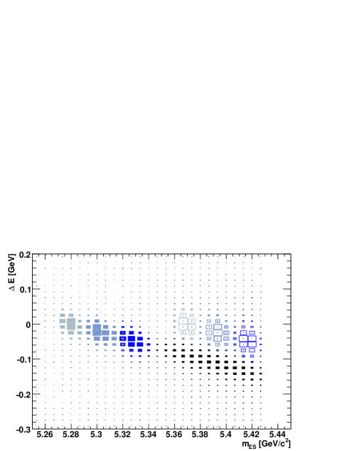
Figure 3: Distribution of $\Delta E$ vs. $m_{ES}$ for a sample of simulated $B_{d,s}\rightarrow J/\psi\phi$ decays at the $\Upsilon(5S)$ resonance. Events coming from $B_{q}^{(*)}\bar{B}_{q}^{(*)}$ ($q=d,s$) are all generated with the same relative rate. We use full boxes for $q=d$ and empty boxes for $q=s$. The color scale identifies VV, VP and PP events (from the darker to the lighter). Events from $B_{d}\bar{B}_{d}\pi$ events are also shown (full dark boxes on the bottom-right).

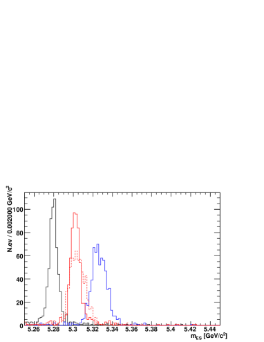
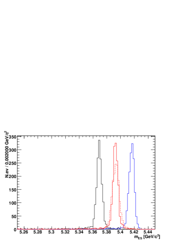
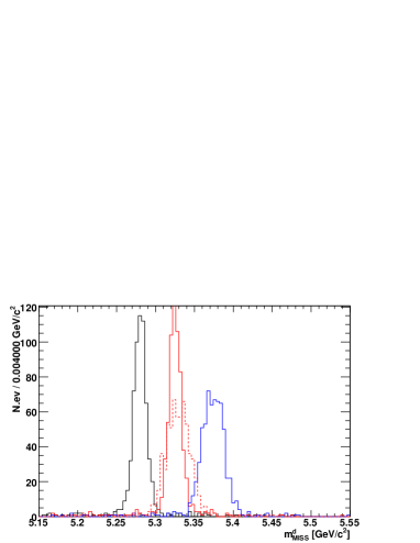
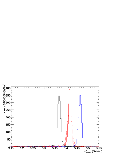
Figure 4: Top row : distribution of $m_{ES}$ for a sample of simulated $B_{d}$ (left) and $B_{s}$ (right) decaying to $J/\psi\phi$ at the $\Upsilon(5S)$ resonance. Bottom row : distribution of $m^{d}_{miss}$ for a sample of simulated $B_{d}$ (left) and $m^{s}_{miss}$ for a sample of $B_{s}$ (right) decaying to $J/\psi\phi$ at the $\Upsilon(5S)$ resonance. From the left to right, we show events coming from $B_{q}B_{q}$, $B_{q}B^{*}_{q}$, $B^{*}_{q}B_{q}$ (dashed) and $B^{*}_{q}B^{*}_{q}$ ($q=d,s$), all generated with the same relative rate. In writing $B^{(*)}_{q}B^{(*)}_{q}$ the first $B^{(*)}_{q}$ is intended as the reconstructed one.

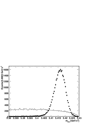
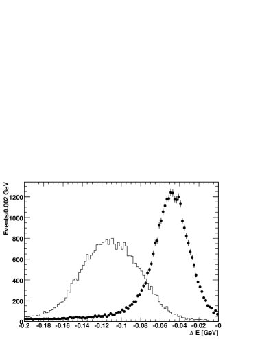
Figure 5: Distribution of $m_{ES}$ (left) and $\Delta E$ (right) for $B_{d}\rightarrow J/\psi\phi$ candidates, from a sample of simulated $\Upsilon(5S)\rightarrow B_{d}\bar{B}_{d}\pi$ events (line). $B_{s}\rightarrow J/\psi\phi$ events, generated in $\Upsilon(5S)\rightarrow B_{s}^{*}\bar{B}_{s}^{*}$ events (dots), are also shown for comparison.

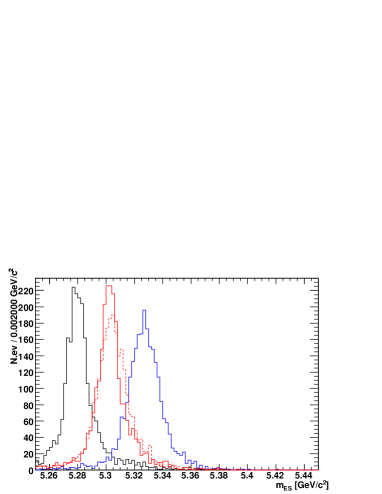
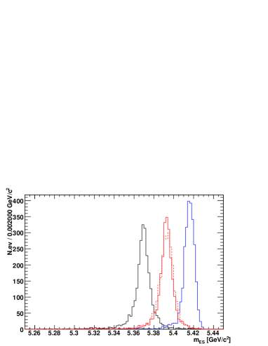
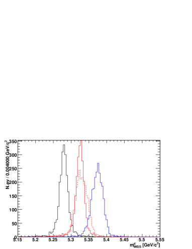
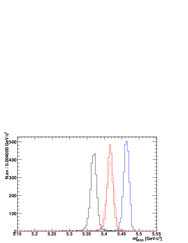
Figure 6: Top row : distribution of $m_{ES}$ for a sample of simulated $B_{d}$ (left) and $B_{s}$ (right) decaying to $K^{0}_{S}\pi^{0}$ at the $\Upsilon(5S)$ resonance. Bottom row : distribution of $m^{d}_{miss}$ for a sample of simulated $B_{d}$ (left) and $m^{s}_{miss}$ for a sample of $B_{s}$ (right) decaying to $K^{0}_{S}\pi^{0}$ at the $\Upsilon(5S)$ resonance. From the left to right, we show events coming from $B_{q}B_{q}$, $B_{q}B^{*}_{q}$, $B^{*}_{q}B_{q}$ (dashed) and $B^{*}_{q}B^{*}_{q}$ ($q=d,s$), all generated with the same relative rate. In writing $B^{(*)}_{q}B^{(*)}_{q}$ the first $B^{(*)}_{q}$ is intended as the reconstructed one.

3.1 Selection of $B_{d,s}\rightarrow J/\psi\phi$

Fig. 3 shows the distribution of signal Monte Carlo events for $B_{d,s}\rightarrow J/\psi\phi$ decays, obtained assuming all the $b\bar{b}$ decays of the $\Upsilon(5S)$ to have the same production rate. The values of the two variables are calculated from the daughters of the reconstructed $B$ mesons, without searching for additional particles (photons or pions) produced in the $\Upsilon(5S)$ decay tree.

It can be noted that the PP, PV and VV configurations are well separated in the ($m_{ES}$,$\Delta E$) plane. $B_{d,s}B_{d,s}$ events are centered at $\Delta E\sim 0$ while $B_{d,s}B_{d,s}^{\ast}$ and $B_{d,s}^{\ast}B_{d,s}^{\ast}$ are shifted to negative values of $\Delta E$ and higher values of $m_{ES}$ due to the missing energy of the photons originating from $B_{s}^{*}\rightarrow B_{s}\gamma$ decays. In a similar way, $B\bar{B}\pi$ events are further shifted. Three important features should be noted:

• The resolution of both variables is worse in the case of $B_{d}$ mesons than for $B_{s}$ mesons, since $B_{d}$ mesons receive a larger momentum than $B_{s}$ mesons in the CM frame of the $\Upsilon(5S)$, resulting in a wider distribution of the $B$ momentum in the laboratory frame.

• The resolution for VV events is worse than for PP ones, since the presence of the photon introduces an additional source of energy spread.

• In the case of PV events, the distribution is the sum of two components: a broad one, due to reconstructed $B$ mesons originating from the $B^{*}$ decay; and a narrow one, due to reconstructed $B$ mesons originating directly from the $\Upsilon(5S)$. This is shown in Fig 4, where the two components are independently shown in the $m_{ES}$ and $m_{miss}$ projections.

We consider only VV events and we study the cross-feed generated by the tails of similar events (in this case $B_{d,s}\rightarrow J/\psi\phi$) coming from the other configurations (PP and PV). We have chosen specific selection criteria for $m_{ES}$ or $m_{miss}$ to separate the different components. We find that in general, and mainly for the channels with photons in the final state as shown in the following sections, the $m_{miss}$ variables provide better efficiency and purity. In Tab. 2 we summarize the cuts applied on $m_{miss}$, the efficiency and we quantify the cross-feed among $B_{s}$ and $B_{d}$ samples.

The situation is different in the case of $B\bar{B}\pi$ continuum production. These events are overlapped to $B_{s}$ mesons from VV events, in such a way that a simple cut in the $\Delta E$ vs. $m_{ES}$ plane cannot separate the two components without affecting the distribution of $q\bar{q}$ background.

The separation is indeed possible since these events are characterized by a continuum-like distribution in $m_{ES}$ (see left plot of Fig. 5), while they exhibit a peaking structure in $\Delta E$ (see right plot of Fig. 5), shifted to negative values with respect to $B_{s}$ mesons, because of the undetected energy of the pion. At present, concerning the relative amount of this component with respect to $B_{s}$ mesons, we can rely only the upper limit (UL) quoted by CLEO [15] (see Tab. 1), so that we are not allowed to neglect this kind of background. Anyhow, the differences in the kinematic variables allow to isolate these events from the signal, adding a component in the Maximum Likelihood (ML) fit as it is currently done with $B\bar{B}$ background in many charmless analyses in BaBar [22].

	$B_{d}$	$B_{s}$
	$B\rightarrow J/\psi\phi$
Cut	$5.355<m^{d}_{miss}\,[GeV]<5.410$	$5.440<m^{s}_{miss}\,[GeV]<5.490$
Efficiency	81%	91%
Contamination	1.1%	0.0%
	[PV=0.7%, PP=0.3%]
	$B\rightarrow K^{0}_{S}\pi^{0}$
Cut	$5.350<m^{d}_{miss}\,[GeV]<5.410$	$5.440<m^{s}_{miss}\,[GeV]<5.490$
Efficiency	89%	98%
Contamination	1.6%	0.0%
	[PV=1.5%, PP=0.1%]
	$B\rightarrow K^{*}(K^{0}_{S}\pi^{0})\gamma$
Cut	$5.355<m^{d}_{miss}\,[GeV]<5.410$	$5.440<m^{s}_{miss}\,[GeV]<5.490$
Efficiency	75%	84%
Contamination	4.4%	0.5%
	[PV=3.3%, PP=1.0%]	[PV=0.4%, PP=0.1%]

Table 2: Cuts, efficiencies and contaminations in the channels $B\rightarrow J/\psi\phi$ (no photons), $B\rightarrow K^{0}_{S}\pi^{0}$ (2 photons), $B\rightarrow K^{*}\gamma$ (3 photons). The quoted values take into account the different production rates of the $\Upsilon(5S)$ resonance. The contamination of $B_{d}$ to $B_{s}$ ($B_{s}$ to $B_{d}$) is negligible (less than $0.1\%$).

3.2 Selection of $B_{d,s}\rightarrow K^{0}_{S}\pi^{0}$

As mentioned in Sec. 3, the presence of neutral particles in the final state smears the distribution of the interesting kinematic variables. The ability of the cuts to separate the different channels is therefore reduced by this effect, so that the result of the previous study is not guaranteed to hold in this case. To investigate this point, we consider a sample of $B_{d,s}\rightarrow K^{0}_{S}\pi^{0}$ decays, reconstructing signal candidates from $K^{0}_{S}\rightarrow\pi^{+}\pi^{-}$ and $\pi^{0}\rightarrow\gamma\gamma$ decays.

Fig. 6 shows the $m_{ES}$, $m^{d}_{miss}$ and $m^{s}_{miss}$ distributions in this channel. Although the width of the distribution increases in a significant way, it is still possible to separate the different contributions. In particular, the use of $m^{d}_{miss}$ rather than $m_{ES}$ provides a separation almost as good as in the case of $J/\psi\phi$ final states.

3.3 Selection of $B_{d,s}\rightarrow K^{*}\gamma$

As a further step, we repeat the previous study using $B_{d,s}\rightarrow K^{*}(K^{0}_{S}\pi^{0})\gamma$ signal events, reconstructed from $K^{0}_{S}\rightarrow\pi^{+}\pi^{-}$ and $\pi^{0}\rightarrow\gamma\gamma$. In this case, there are three photons in the final state. As in the previous section, an improvement in the separation between different channels can be achieved using $m_{miss}$ instead of $m_{ES}$. In Tab. 2, we summarize the cuts applied on $m_{miss}$ in the three channels, with efficiencies and the details on the contaminations.

3.4 A Remark on $B$ reconstruction

We would like to highlight a point that is relevant for the rest of this paper. Since it is possible to isolate $B_{s}$ mesons from $B_{d}$ and charged $B$ mesons, it is clear that it is possible to continue the $\Upsilon(4S)$ physics program when running at the $\Upsilon(5S)$. This is particularly crucial for measurements that are difficult to perform at other facilities, such as inclusive measurements ($b\rightarrow s\gamma$, $b\rightarrow sll$, and semileptonic decays) as well as some exclusive measurements with open kinematic ($B\rightarrow\tau\nu$, exclusive semileptonic decays). All these measurements represent important milestones of the physics program of the current $B$-Factories and it is hard to imagine a precision test of the flavour sector of NP without the possibility of reducing the errors on these observables with future facilities. At the same time, as already stressed in Sec. 2, one should keep in mind that there is a price to pay in terms of statistics, corresponding to a factor about three (six) for inclusive (exclusive) measurements.

4 Accessing CP asymmetries in $B^{0}_{d}$–$\bar{B}^{0}_{d}$ events

In order to cover the physics program of a $B$-Factory running at the $\Upsilon(4S)$ resonance, not only one should be able to identify $B_{d}$ and charged $B$ mesons, but also to perform time-dependent measurements of CP asymmetries in $B_{d}$ decays, which are based on the fact that the initial $B\bar{B}$ pair is produced in a coherent state. Moving to the $\Upsilon(5S)$ does not bring problems in terms of vertexing and tagging, since the experimental environment is similar to that of BaBar and Belle. In addition, as for the $\Upsilon(4S)$, the $B_{d}\bar{B}_{d}$ pair is in a coherent state when the $\Upsilon(5S)$ decays in a PP final state. We show below that this is also true for the dominant contribution, namely VV decays. We also discuss how, using time-integrated measurements, PV decays could be used to access the value of ${\mathcal{I}m}\lambda^{f}_{CP}$, with $\lambda^{f}_{CP}=\frac{q}{p}\frac{\bar{A}_{f}}{A_{f}}$.

This last feature represent a novelty with respect to the study of $\Upsilon(4S)$ decays and it allows to obtain an information equivalent to the measurement of the coefficient $S$ of the time-dependent CP asymmetry even for those decays for which a measurement of the $B$ decay vertex, needed for time-dependent measurements, cannot be performed. This is for instance the case of $B_{d}\rightarrow\pi^{0}\pi^{0}$ and $B_{d}\rightarrow\gamma\gamma$ decays, for which otherwise only $\gamma$ conversion processes would allow to try a time-dependent measurement, paying a big price in terms of reconstruction efficiency.

4.1 The coherent time evolution of the $B^{*}\bar{B}^{*}$ mesons

As explained in Sec. 2, at the $\Upsilon(5S)$ resonance $B^{*}\bar{B}^{*}$ meson pairs are produced in a $J^{CP}=1^{--}$ state. The question is whether the $B_{q}\bar{B}_{q}$ pairs resulting from the $B_{q}^{*}\rightarrow B_{q}\gamma$ and $\bar{B}_{q}^{*}\rightarrow\bar{B}_{q}\gamma$ decays exhibit the same properties of quantum coherence of the initial state. Since the $B_{q}^{*}\rightarrow B_{q}\gamma$ decay (and its CP conjugate) is an electromagnetic decay and can be considered instantaneous, one is allowed to regard the $B_{q}\bar{B}_{q}\gamma\gamma$ final state as a direct product of the $\Upsilon(5S)$ resonance. This implies that the state constituted by these four final particles has to preserve the initial quantum numbers. Since the two photons have to satisfy the Bose-Einstein statistic, their sum has to be a symmetric state. This request forces the $B_{q}\bar{B}_{q}$ pairs to be in an antisymmetric state. This implies that $B_{q}\bar{B}_{q}$ pairs produced in a VV event of a $\Upsilon(5S)$ decay have the same quantum coherence properties of $B^{0}\bar{B}^{0}$ pairs generated at the $\Upsilon(4S)$ resonance. The full expression for the decay amplitude is:

$$A^{\mu} =B_{s}(p_{1}+k_{1})\cdot B_{s}(p_{2}+k_{2})\cdot G_{3}\cdot$$

$$\cdot\Big{(}\frac{\epsilon(q,p_{1},k_{1},\epsilon_{1})\epsilon(q,p_{2},k_{2},\epsilon_{2})p_{1}^{\mu}}{2M_{B_{s}^{\ast}}^{2}}-\frac{\epsilon(q,p_{1},k_{1},\epsilon_{1})\epsilon(q,p_{2},k_{2},\epsilon_{2})p_{2}^{\mu}}{2M_{B_{s}^{\ast}}^{2}}+$$

$$+\frac{\epsilon(q,p_{1},k_{1},\epsilon_{1})\epsilon(q,p_{2},k_{2},\epsilon_{2})k_{1}^{\mu}}{2M_{B_{s}^{\ast}}^{2}}-\frac{\epsilon(q,p_{1},k_{1},\epsilon_{1})\epsilon(q,p_{2},k_{2},\epsilon_{2})k_{2}^{\mu}}{2M_{B_{s}^{\ast}}^{2}}\Big{)}+$$

$$+B_{s}(p_{1}+k_{1})\cdot B_{s}(p_{2}+k_{2})\cdot G_{2}\cdot$$

$$\cdot\Big{(}-\epsilon(q,p_{1},k_{1},\epsilon_{1})\epsilon(p_{2},k_{2},\epsilon_{2},\mu)+\epsilon(q,p_{2},k_{2},\epsilon_{2})\epsilon(p_{1},k_{1},\epsilon_{1},\mu)+$$

$$+2\epsilon(p_{1},k_{1},\epsilon_{1},\sigma)\epsilon(p_{2},k_{2},\epsilon_{2},\sigma)p_{1}^{\mu}-2\epsilon(p_{1},k_{1},\epsilon_{1},\sigma)\epsilon(p_{2},k_{2},\epsilon_{2},\sigma)p_{2}^{\mu}+$$

$$+2\epsilon(p_{1},k_{1},\epsilon_{1},\sigma)\epsilon(p_{2},k_{2},\epsilon_{2},\sigma)k_{1}^{\mu}-2\epsilon(p_{1},k_{1},\epsilon_{1},\sigma)\epsilon(p_{2},k_{2},\epsilon_{2},\sigma)k_{2}^{\mu}\Big{)}+$$

$$+B_{s}(p_{1}+k_{2})\cdot B_{s}(p_{2}+k_{1})\cdot G_{3}\cdot$$

$$\cdot\Big{(}\frac{\epsilon(q,p_{1},k_{2},\epsilon_{2})\epsilon(q,p_{2},k_{1},\epsilon_{1})p_{1}^{\mu}}{2M_{B_{s}^{\ast}}^{2}}-\frac{\epsilon(q,p_{1},k_{2},\epsilon_{2})\epsilon(q,p_{2},k_{1},\epsilon_{1})p_{2}^{\mu}}{2M_{B_{s}^{\ast}}^{2}}-$$

$$-\frac{\epsilon(q,p_{1},k_{2},\epsilon_{2})\epsilon(q,p_{2},k_{1},\epsilon_{1})k_{1}^{\mu}}{2M_{B_{s}^{\ast}}^{2}}+\frac{\epsilon(q,p_{1},k_{2},\epsilon_{2})\epsilon(q,p_{2},k_{1},\epsilon_{1})k_{2}^{\mu}}{2M_{B_{s}^{\ast}}^{2}}\Big{)}+$$

$$+B_{s}(p_{1}+k_{2})\cdot B_{s}(p_{2}+k_{1})\cdot G_{2}\cdot$$

$$\cdot\Big{(}-\epsilon(q,p_{1},k_{2},\epsilon_{2})\epsilon(p_{2},k_{1},\epsilon_{1},\mu)+\epsilon(q,p_{2},k_{1},\epsilon_{1})\epsilon(p_{1},k_{2},\epsilon_{2},\mu)+$$

$$+2\epsilon(p_{1},k_{2},\epsilon_{2},\sigma)\epsilon(p_{2},k_{1},\epsilon_{1},\sigma)p_{1}^{\mu}-2\epsilon(p_{1},k_{2},\epsilon_{2},\sigma)\epsilon(p_{2},k_{1},\epsilon_{1},\sigma)p_{2}^{\mu}-$$

$$-2\epsilon(p_{1},k_{2},\epsilon_{2},\sigma)\epsilon(p_{2},k_{1},\epsilon_{1},\sigma)k_{1}^{\mu}+2\epsilon(p_{1},k_{2},\epsilon_{2},\sigma)\epsilon(p_{2},k_{1},\epsilon_{1},\sigma)k_{2}^{\mu}\Big{)},$$ (2)

where

$$B_{s}(P)=\frac{1}{P^{2}-M_{B_{s}^{\ast}}^{2}+iM_{B_{s}^{\ast}}\Gamma_{B_{s}^{\ast}}}$$

$$\epsilon(a,b,c,d)=\epsilon_{\alpha\beta\gamma\delta}a^{\alpha}b^{\beta}c^{\gamma}d^{\delta}=\epsilon^{\alpha\beta\gamma\delta}a_{\alpha}b_{\beta}c_{\gamma}d_{\delta}$$

$$\epsilon(a,b,c,\sigma)\epsilon(d,e,f,\sigma)=\epsilon_{\alpha\beta\gamma\sigma}\epsilon^{\delta\lambda\nu\sigma}a^{\alpha}b^{\beta}c^{\gamma}d_{\delta}e_{\lambda}f_{\nu},$$ (3)

and $\mu$ is the index contracted by the $\Upsilon(5S)$ polarization vector, $q$ is the $\Upsilon(5S)$ momentum, $p_{1}(p_{2})$ is the $B_{s}(\bar{B}_{s})$ momentum, $k_{1}$ and $k_{2}$ ($\epsilon_{1}$ and $\epsilon_{2}$) are the photons momenta (polarization vectors), and $G_{2}$ and $G_{3}$ are two hadronic form factors  [23] . Among the variables entering Eq. (2) and Eq. (3), $G_{2}$ and $G_{3}$ are the only whose knowledge is not precise. Different estimates exist in literature [23, 24], but at present the theoretical expectation is controversial. Anyhow, since the ratio of the two determines the angular distribution of the $B^{*}\bar{B}^{*}$ mesons (and so also of the $B_{q}\bar{B}_{q}$ pairs) in the $\Upsilon(5S)$ rest frame, the study of the angular distribution of the final states in $\Upsilon(5S)$ decays allows to experimentally ascertain them. In any case, whatever the value of the two form factors is, the coherence of the $B_{q}\bar{B}_{q}$ is guaranteed by Eq. (2).

4.2 Time-integrated CP asymmetries in $B^{*}B$ events

When the $\Upsilon(5S)$ decays to $B^{*}\bar{B}$ events, the final $B\bar{B}$ system is in a C$=+1$ state, after the decay $B^{*}\rightarrow B\gamma$. This difference implies that, unlike the case of $\Upsilon(4S)$, for each value of the time $t$, before one of the two $B$ mesons decays, the two mesons are both $B_{H}$ or $B_{L}$ CP eigenstates. Integrating the time out of the wave function of the $B\bar{B}$ pair, the time-integrated CP asymmetry becomes [25]:

$$A^{f}_{CP}=\left(\frac{1-y^{2}}{1+x^{2}}\right)^{2}\frac{(1-x^{2})(1-|\lambda^{f}_{CP}|^{2})+4x{\mathcal{I}m}(\lambda^{f}_{CP})}{(1+y^{2})(1+|\lambda^{f}_{CP}|^{2})-4y{\mathcal{R}e}(\lambda^{f}_{CP})}$$ (4)

where $x=\Delta m/\Gamma$, $y=\Delta\Gamma/2\Gamma$, $\lambda^{f}_{CP}=\frac{q}{p}\frac{\bar{A}_{f}}{A_{f}}$, $q/p$ is the mixing parameter of the $B$–$\bar{B}$ mixing, $A_{f}$ ($\bar{A}_{f}$) is the amplitude for $B\rightarrow f$ ($\bar{B}\rightarrow f$) decays, and $\eta_{f}$ is the CP eigenvalue of the final state $f$.

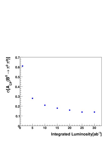
Figure 7: Statistical error on the measurement of $A_{CP}(B_{d}\rightarrow\pi^{0}\pi^{0})$ for PV decays collected at the $\Upsilon(5S)$, as a function of the integrated luminosity.

While this might not be relevant for those channels for which $\lambda^{f}_{CP}$ can be determined at the $\Upsilon(4S)$, it opens new perspectives in the study of CP asymmetries for $B_{d}$ decays to neutral particles, among which two remarkable examples are $B_{d}\rightarrow\gamma\gamma$ and $B_{d}\rightarrow\pi^{0}\pi^{0}$. $B_{q}\rightarrow\gamma\gamma$ decays are sensitive to NP effects in $b\rightarrow q$ transitions and they are complementary to the measurement of $b\rightarrow q\gamma$ processes (see Sec. 6.3). We do not discuss this specific case, while we concentrate our attention to the impact of measuring the direct CP asymmetry of $B_{d}\rightarrow\pi^{0}\pi^{0}$ decays in PV events.

Measurements of rate and asymmetry of $B_{d}\rightarrow\pi^{0}\pi^{0}$ are currently used in the isospin analysis of $B\rightarrow\pi\pi$ decays for extracting $\alpha$. The isospin analysis provides eight solutions, corresponding to the trigonometric ambiguities of the isospin construction [26]. Recently, it was shown that the use of basic QCD properties allows to exclude some of the solutions [27], still leaving several ambiguities in the determination of $\alpha$. The measurement of ${\mathcal{I}m}(\lambda^{f}_{CP})$ from Eq. (4) allows to remove some of these ambiguities, providing an additional information with respect to BR’s and CP asymmetries of the other channels.

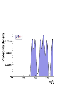
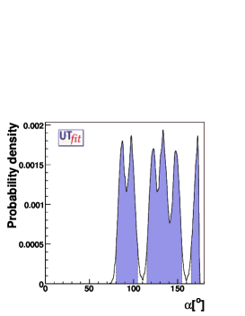
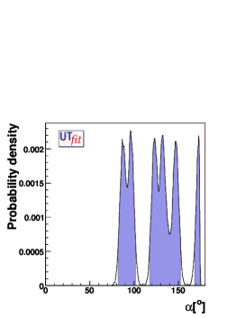
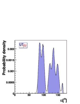
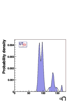
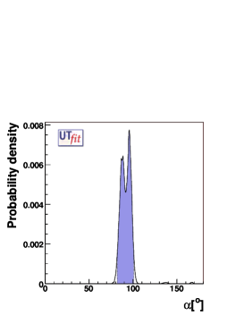
Figure 8: Determination of the angle $\alpha$ without (top) or with (bottom) the constrain from direct CP asymmetries of $B_{d}\rightarrow\pi\pi$ decays in PV events, combining 1 ab^-1(left), 5 ab^-1(center) and 30 ab^-1(right) integrated at the $\Upsilon(5S)$ for 2 ab^-1 collected at the $\Upsilon(4S)$ (end of BaBar and Belle data taking).

From an experimental point of view, the determination of the direct CP asymmetry in PV decays is equivalent to what is done at the $\Upsilon(4S)$ for the same decay channel [28]. Using kinematic cuts and requirements on the energy deposits in the electromagnetic calorimeter, signal events are isolated from continuum background in a ML fit that uses topological and kinematic variables. Using the information obtained applying the tagging algorithm on the rest of the event, the flavour of the decaying $B$ meson is determined on a statistical basis, taking into account the misidentification probability of the tagging algorithm. Scaling the currently available BaBar result to the statistics available at a $B$-Factory machine running at the $\Upsilon(5S)$ and assuming the same tagging performances, we obtain the experimental error as a function of the luminosity shown in Fig. 7.

To illustrate the impact of this measurement on the isospin analysis, we implemented this new measurement in both $B_{d}\rightarrow\pi^{0}\pi^{0}$ and $B_{d}\rightarrow\pi^{+}\pi^{-}$ modes in the analysis by ${\bf UT}fit$ [27]. The measurements currently available will be improved using VV (PV and VV) events for CP asymmetries (decay rates). We assume also that the results of the $\Upsilon(5S)$ runs will be combined to the outcome of 2 ab^-1 collected by BaBar and Belle at the end of their data taking. At the same time, the measurement of direct CP asymmetry for neutral $B$ decays in PV events will provide the experimental determination of the observable in Eq. (4). While $A_{CP}(\pi^{0}\pi^{0})$ provides a new information, with respect to what is currently used in the isospin analysis, $A_{CP}(\pi^{+}\pi^{-})$ contributes to reduce the error on ${\mathcal{I}m}(\lambda_{CP})(\pi^{+}\pi^{-})$, already constrained by $S(\pi^{+}\pi^{-})$. For all the measurements, we use the current central values and the errors are obtained scaling the statistical errors to the assumed luminosity, without reducing the systematic error. The error on the measurements of direct CP asymmetries in PV decays are obtained scaling those of PP decays to the ratio of relative production fractions (see Tab. 1).

The result in terms of the determination of the angle $\alpha$ is shown in Fig. 8 using the current isospin analysis (top) and adding the information from PV decays (bottom), for three different values of integrated luminosities. The plots clearly show that the ambiguity is substantially reduced already with 5 ab^-1 of integrated data.

5 Accessing the $B^{0}_{s}$–$\bar{B}^{0}_{s}$ mixing phase

One of the main ingredients of the success of the current $B$-Factories is the possibility of using the coherence of the initial $B$–$\bar{B}$ state to exploit the interference between CP violation in the decay and in the mixing. Thanks to this technique the measurement of $\sin 2\beta$ has been possible with a high level of accuracy.

In the same way, one would like to exploit the coherence of the $B^{*}_{s}$–$\bar{B}^{*}_{s}$ final state at $\Upsilon(5S)$. The paradigmatic physics goal in this field is the determination of the weak phase $\beta_{s}$ using $B_{s}\rightarrow J/\psi\phi$ decays.

As described in the following, this does not seem achievable with the precision of the current vertexing detectors and the design parameters of the next-generation $B$-Factories, currently under discussion [13]. The main problem comes from the large value of the ratio $\Delta m_{s}/\Delta m_{d}=35.0\pm 0.4$, which requires a presently unreachable vertexing resolution to be sensitive to $B_{s}$ oscillations.

Nevertheless, information on the mixing phases can still be obtained using time-integrated measurements. In general, comparing the tagged decay rates for $B_{s}$ decays into CP eigenstates $f$ for positive and negative values of $\Delta t$, it is possible to determine the value of ${\mathcal{R}e}\lambda^{f}_{CP}$ and ${\mathcal{I}m}\lambda^{f}_{CP}$. Considering different decay modes, several combinations of weak phases can be extracted. In particular, we consider the case of the determination of $\beta_{s}$ from tree-level $B^{0}\rightarrow J/\psi\phi$ decays and from penguin dominated $B_{s}\rightarrow K^{0}\bar{K}^{0}$ decays. In addition, complementary information on $\beta_{s}$ can be obtained from the charge asymmetry in flavour specific final states or in dimuon events, or from the angular analysis of $B^{0}\rightarrow J/\psi\phi$ decays.

5.1 Time-dependent CP asymmetry

The study of time-dependent CP asymmetries is one of the milestones of the physics program for currently running $B$-Factories. It is based on the simple idea that, provided that the laboratory frame is sufficiently boosted with respect to the CM frame of the $\Upsilon$ resonance, it is possible to access the $B_{q}$ oscillation even though the vertex resolution is smaller than $\Delta m_{q}$, thanks to the $\beta\gamma$ Lorentz factor [29]. In the case of $B_{d}$–$\bar{B}_{d}$ oscillation, a boost of $\beta\gamma\sim 0.5$ was large enough to allow the measurement of $\sin 2\beta$ with the vertex precision available when BaBar and Belle were designed. With the currently available technology on silicon vertex detectors, the boost could be in principle reduced by a factor of two or the resolution improved by the same factor using the current boost. Nevertheless, this is not enough for $B_{s}$–$\bar{B}_{s}$ oscillations, which are too much faster than in the case of $B_{d}$ mesons.

We used Monte Carlo simulated experiments (toy Monte Carlo experiments) to identify the minimal vertexing resolution needed to detect $B_{s}$–$\bar{B}_{s}$ oscillations at a $B$-Factory. We quantify the minimal resolution as the largest value of the $\Delta t$ resolution that allows to extract the $S$ and $C$ parameters of the time-dependent CP asymmetry of $B_{s}\rightarrow J/\psi\phi$ decays with an accuracy comparable to the precision on $\sin 2\beta$. In this way, it is possible to provide an answer to the problem without necessarily relying on a particular set of machine and detector parameters. The result obtained can then be translated into a requirement on a given machine, once the energies of the beams (that fix the Lorentz boost) are defined. In fact, the precision on $\sigma(\Delta t)$ can be written in terms of the resolution of the vertex detector $\sigma(\Delta z)$ and the Lorentz boost $\beta\gamma$ of the CM frame with respect to the laboratory frame, by using the relation $\sigma(\Delta z)\sim\sigma(\Delta t)\beta\gamma c$.

We determine the shape of signal and background using fully simulated samples, selected requiring [30]:

• $3.06$ GeV $<m_{J/\psi}<3.14$ GeV for $J/\psi\rightarrow\mu^{+}\mu^{-}$

• $2.95$ GeV $<m_{J/\psi}<3.14$ GeV for $J/\psi\rightarrow e^{+}e^{-}$

• $1.004$ GeV $<m_{\phi}<1.034$ GeV

• particle identification (PID) requirements based on Cherenkov angle and $dE/dx$, both on $J/\psi$ and $\phi$ daughters.

• a cut on the polar angle of the thrust axis: $|\cos(\theta_{Thr})|<0.8$

in order to reduce contamination from $q\bar{q}$ background and from tracks combinatoric. We also apply the following kinematic requirements:

• $5.440$ GeV $<m^{s}_{miss}<5.490$ GeV

• $-0.2$ GeV $<\Delta E<0.1$ GeV

to select an almost pure sample of $\Upsilon(5S)\rightarrow B_{s}^{*}B_{s}^{*}$ events. This selection has a global efficiency of $\sim 14.7\%$ on signal events. We generate and fit samples containing signal and background events (scaled to the considered luminosity), according to the following likelihood function:

$${\mathcal{L}}=\frac{e^{-(N_{sig}+N_{bkg})/N}}{{}^{N}\sqrt{(N_{sig}+N_{bkg})!}} \cdot \prod_{i=1}^{N}\{N_{sig}\cdot P_{sig}(m_{miss})_{i}\cdot P_{sig}(\Delta E)_{i}\cdot P_{sig}({\cal F})_{i}\cdot P_{sig}(\Delta t)_{i}+$$ (5)

$$N_{bkg}\cdot P_{bkg}(m_{miss})_{i}\cdot P_{bkg}(\Delta E)_{i}\cdot P_{bkg}({\cal F})_{i}\cdot P_{bkg}(\Delta t)_{i}\},$$

where $P_{sig}(x)$ ($P_{bkg}(x)$) is the probability density function (PDF) of the variable $x$ for the signal ($q\bar{q}$ background) component. Background events from other $B\bar{B}$ decays are negligible after the selection cuts. $P_{sig}(\Delta t)$ takes into account the knowledge of the proper time of $B$ mesons, coming from the vertex reconstruction. The full expression uses the convolution of the angular distribution function with the resolution function associated to the vertex reconstruction (usually, the sum of three Gaussians, with mean and width scaled according to the per-event error $\sigma_{\Delta t}$). We assumed the models adopted for BaBar time-dependent measurements [31], for both the shape of $\Delta_{t}$ and the performances of the tagging algorithm.

All the other functions are used to separate signal from background. Their shapes are obtained from unbinned maximum-likelihood fits to signal and background samples, coming from full Monte Carlo simulations.

The signal distributions for $m_{miss}^{s}$, $\Delta E$, and the Fisher discriminant ${\cal F}$ are parameterized as:

$$f(x)=\exp\Big{[}-\frac{(x-m)^{2}}{2\sigma^{2}_{\pm}+\alpha_{\pm}(x-m)^{2}}\Big{]}$$ (6)

where $m$ is the maximum of the distribution, while $\sigma_{\pm}$ and $\alpha_{\pm}$ quantify the width and the tail, the positive (negative) sign corresponding to positive (negative) values of $x-m$. The invariant masses of the two resonances, $m_{\phi}$ and $m_{J/\psi}$ are described by relativistic Breit-Wigner functions.

In order to describe the $q\bar{q}$ background, we use a second-order polynomial for $\Delta E$, while ${\cal F}$ is given by the function of Eq. (6) and $m_{miss}^{s}$ is parameterized by a phase-space threshold function [34]:

$$f(x)=x\sqrt{1-x^{2}}\exp\Big{[}-\xi\cdot(1-x^{2})\Big{]}~{}~{}~{}~{}~{};~{}~{}~{}~{}~{}~{}x=m_{miss}^{s}/m_{T}$$ (7)

where $m_{T}$ is the value of the threshold and $\xi$ is the parameter determining the shape. For $\Delta t$ we use a Gaussian resolution function.

The $B_{d}$ background is parameterized using the function of Eq. (6) for $\Delta E$, and the phase-space threshold function (as in Eq. (7)) for $m_{miss}^{s}$. All the other PDF’s are similar to signal ones.

For simplicity, we assume a fully polarized final state, which allows us to discard from the likelihood the PDF describing the angular distribution, and we parameterize the resolution function with a single Gaussian function, centered around $-0.2$ ps^-1 (to include the effect of the charm bias on the tag side). Here, we do not use the per-event error but an average value $\sigma_{\Delta t}$ as the RMS of the resolution function, varied in the range [0.02,0.20] ps^-1. We assume an integrated luminosity of $30~{}ab^{-1}$ and we generate and fit a set of toy Monte Carlo samples for each value of $\sigma_{\Delta t}$. The result of this study is reported in Fig. 9 for the error on $S$. The error on $C$ is not shown, since the values of the errors on $S$ and $C$ are the same for all the chosen values of $\sigma_{\Delta t}$.

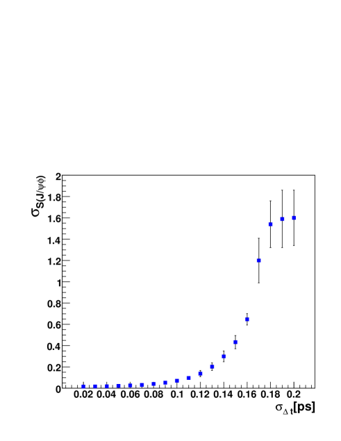
Figure 9: Error on $S(J/\psi\phi)$ as a function of the $\Delta t$ resolution $\sigma_{\Delta t}$. Error bars represent the RMS of the error distribution for a given set of toys.

It is clear from the plot that, in order to achieve an acceptable precision on the value of the CP parameters, values of $\sigma(\Delta t)\leq 0.11$ ps are needed. We also found that for values larger than $0.11$ ps not only the average error increases, but also a bias is introduced in the fit, generating a larger spread in the error distribution (the error bars in the plot). For these values of $\sigma(\Delta t)$ the $B_{s}$ oscillation is too fast to be detected. The bad news is that the values of resolution required are beyond the possibilities of the current designs. The existing $B$-Factories are outside the range of the plot, having $\sigma(\Delta t)\sim 0.65$ ps. The improvements coming from new technology, together with the possibility of adding to the vertex detector a layer 0 [8] on top of the beam pipe, allows to push $\sigma(\Delta t)$ down to $\sim 0.4$ ps for a boost of $\beta\gamma\sim 0.28$ [35], corresponding to $\sim 0.2$ ps for a boost of $\beta\gamma\sim 0.6$.

We stress the fact that statistics alone does not allow to reduce the errors in a significative way, since the limiting factor is in the vertexing resolution and does not have a statistical nature (as for instance in the case of decay modes with large backgrounds).

5.2 Tagged rates at positive and negative $\Delta t$

Even assuming that the needed time resolution for the study of $B_{s}$–$\bar{B}_{s}$ oscillations is outside the capability of the next-generation $B$-Factories, it remains possible to measure weak phases in $B_{s}$ decays measuring the sign of $\Delta t$ for $B_{s}$–$\bar{B}_{s}$ meson pairs. In fact, in this case one can measure decay rates as a function of $B_{s}$ flavour and $\Delta t$ sign, which provide four experimental observables, depending on the weak phase of the chosen final state. Using this technique, it is possible to access the $B_{s}$–$\bar{B}_{s}$ mixing phase $\beta_{s}$ in $B_{s}\rightarrow J/\psi\phi$ decays, as well as combinations of this phase and the phase $\gamma$ of the CKM matrix (as for the case of $B_{s}\rightarrow D_{s}K$, which we do not discuss here). In this section, we introduce the basic formalism and we provide two examples of such measurements.

5.2.1 Theoretical Formalism and Experimental Details

Let us consider a $B_{s}$ pair produced at the $\Upsilon(5S)$ resonance, through a $B_{s}^{*}\bar{B}_{s}^{*}$ state. If one of the two $B_{s}$ decays into a CP eigenstate with eigenvalue $\eta_{f}$ and the other one in a flavour tagging final state, the PDF of the proper time difference $\Delta t$ can be written as:

$$P(\Delta t)\propto e^{\frac{-|\Delta t|}{\tau}}\left[\kappa_{1}\cosh\left(\frac{\Delta\Gamma_{s}\Delta t}{2}\right)+\kappa_{2}\cos\left(\Delta m_{s}\Delta t\right)+\kappa_{3}\sinh\left(\frac{\Delta\Gamma_{s}\Delta t}{2}\right)+\kappa_{4}\sin\left(\Delta m_{s}\Delta t\right)\right],$$ (8)

where the $\kappa_{i}$ coefficients are defined as:

$$\kappa_{1}=\frac{1}{2}(1+|\lambda^{f}_{CP}|^{2})~{}~{}~{}~{}~{} ~{}~{}~{}~{}~{}\kappa_{2}=-q_{tag}\frac{1}{2}(1-|\lambda^{f}_{CP}|^{2})$$ ;

$$\kappa_{3}=-{\mathcal{R}e}\lambda^{f}_{CP}~{}~{}~{}~{}~{} ~{}~{}~{}~{}~{}\kappa_{4}=-q_{tag}{\mathcal{I}m}\lambda^{f}_{CP}.$$ ; (9)

These four quantities are effective parameters that depend on the tag sign $q_{tag}$ ($+1$ ($-1$) when the tag meson is a $B_{s}$ ($\bar{B}_{s}$)) and on the CP parameter $\lambda^{f}_{CP}$. We use, as a good approximation, $q/p=e^{-2i\beta_{s}}$ in the following.

In the case of the current $B$-Factories, it is usually imposed that $\Delta\Gamma\sim 0$, which holds with a very good accuracy for $B_{d}$ mesons. This assumption reduces the number of parameters to two (the usual $S$ and $C$). In the case of time-integrated measurements, the tagged rates are measured without any requirement on $\Delta t$, which is equivalent to integrating Eq. (8) between $-\infty$ and $\infty$. In the case of time-dependent measurements, the convolution between Eq. (8) and the resolution function of the vertex detector is used in the fit, which allows to extract the $S$ and $C$ coefficients.

As discussed in the previous section, it is hard to imagine that time-dependent measurements of $B_{s}$ decays will be performed at a $B$-Factory. On the other hand, the presence of $\Delta t$-odd terms introduces an asymmetry between the numbers of events with $\Delta t>0$ and $\Delta t<0$, depending on $\lambda^{f}_{CP}$ and $q_{tag}$. In addition, the sign of $\Delta t$ can be determined with good precision even without improving the vertex resolution, since $\tau_{B_{s}}\sim\tau_{B_{d}}$. It is then possible to extract the four parameters $\kappa_{i}$ from the tagged decay rates for positive and negative values of $\Delta t$, the dependence on the $\kappa_{i}$ being provided by the integral of Eq. (8) and the resolution function of the vertex detector in the range $[-\infty,0]$ and $[0,\infty]$. As an alternative, one can measure a flavour integrated rate and quote flavour asymmetries (as currently done by the $B$-Factories), which allows to cancel some of the systematics.

Exploiting the technique described above, it is possible to measure the parameter $\lambda^{f}_{CP}$ for all CP eigenstates of the $B_{s}$, without any need of improving the vertex resolution. Although this procedure is not as powerful as the time-dependent measurements performed by experiments at hadron collider, it can be applied to all the channels for which the $\Delta t$ sign can be detected. Given the very clean environment of $e^{+}$–$e^{-}$ machines, the set of accessible channels is larger than in the case of LHCb. In particular, since the position of the $B$ decay vertex can be measured even using $K^{0}_{S}\rightarrow\pi^{+}\pi^{-}$ rather than prompt tracks [21, 36], the possibility of accessing $\lambda^{f}_{CP}$ even in these cases opens up interesting possibilities.

Covering all the possibilities goes beyond the purpose of this paper. Nevertheless, we give below two examples of the potentiality of this new technique.

5.2.2 Determination of $\beta_{s}$ from tree-level processes

The study of $B_{s}$ decays at hadron colliders allows to determine the absolute value and phase of the $B_{s}$–$\bar{B}_{s}$ mixing amplitude. The comparison of the experimental measurements to the theoretical expectations allows to test the presence of NP in $b\rightarrow s$ transitions. The recent measurement of $\Delta m_{s}$ [10] already provided the first milestone of this physics program. A first measurement of the mixing phase is available from D$\O$ [37], obtained from a time-dependent angular analysis of $B_{s}\rightarrow J/\psi\phi$ decays.

A large improvement will come from LHCb [38]. In fact, this experiment is expected to measure, with the same technique, both the width difference and the phase up to $\sigma(\Delta\Gamma_{s}/\Gamma_{s})=0.0092$ and $\sigma(\beta_{s})=0.023$ [39] in just one year of nominal data taking. With the full expected B physics dataset (10 $fb^{-1}$) the error on $\beta_{s}$ can be reduced to $\sigma(\beta_{s})\simeq 0.01$. It is clear that such a precision cannot be achieved with the Lorentz boost available at present $e^{+}e^{-}$ facilities and the resolution of actual vertexing detectors (see Sec. 5.1). Nonetheless, we will show how a $B$-Factory running at $\Upsilon(5S)$ could provide alternative and independent informations on the same quantities, even if with not the same accuracy.

In fact, one can use the approach described in Sec. 5.2.1 to measure the four $\kappa_{i}$ parameters in the case of $B_{s}\rightarrow J/\psi\phi$ and then extract from them a value for $\beta_{s}$. As for the measurement of $\beta$ from $B_{d}\rightarrow J/\psi K^{0}_{S}$, one can neglect CKM suppressed subleading contributions  and assume that $\lambda^{f}_{CP}=\eta_{f}e^{2i\beta_{s}}$.

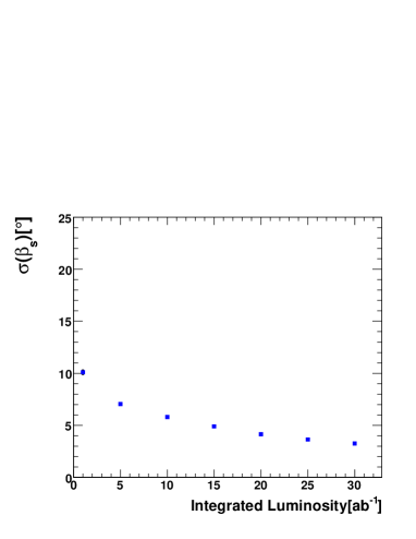
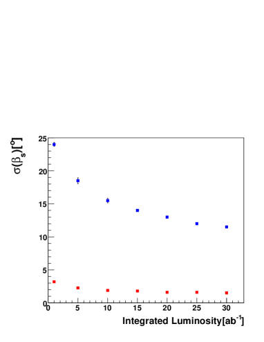
Figure 10: Distribution of the error on $\beta_{s}$ from $B_{s}\rightarrow J/\psi\phi$ (left) and $B_{s}\rightarrow K^{0}\bar{K}^{0}$ (right) decays, as a function of the integrated luminosity, obtained from the measurement of tagged rates with $\Delta t>0$ and $\Delta t<0$. For the right plot, the estimate of the theoretical error is also given (see text for details).

In order to evaluate the sensitivity to $\beta_{s}$, we used the same framework described in Sec. 5.1 to perform a set of toy Monte Carlo experiments, as function of the integrated luminosity. The statistical error as a function of the luminosity, shown in the left plot of Fig. 10, clearly proves the potentiality of this technique and the possibility to measure $\beta_{s}$ with a relatively good precision. We found a two-fold ambiguity between $\beta_{s}$ and $-\beta_{s}$. When the value of . $\beta_{s}$ is close to zero (as it should be in the SM), two different and partially superimposed peaks appear, which produce a (almost) two-times larger resolution in the total pdf. Anyway, it is important to stress that a similar approach can be followed for $B_{s}$ decays into higher charmonium resonances, which provides independent determinations of $\beta_{s}$, taking into account the different hadronic uncertainties.

5.2.3 Determination of $\beta_{s}$ from penguin modes

The same experimental technique can be applied also to determine $\beta_{s}$ from penguin modes. The comparison of this result to the value measured in $B_{s}\rightarrow J/\psi\phi$ allows to test the consistency of the SM and to constrain NP models.

A similar test is usually performed in the $B_{d}$ sector comparing the value of $\sin 2\beta$ from $B_{d}\rightarrow J/\psi K^{0}_{S}$ to the $S$ value of penguin dominated modes, such as $B_{d}\rightarrow\phi K^{0}_{S}$. The equality $(\sin 2\beta)_{J/\psi K^{0}_{S}}=(\sin 2\beta)_{penguin}$ would be strictly true only if these decays were mediated by a single combination of CKM matrix elements, while in all the cases a CKM suppressed amplitude is present. At the very high precision that is expected with the next generation of $B$ physics experiments, it is not be possible to neglect the CKM suppressed contribution, which introduces a theoretical error associated to the SM expectation of $\Delta S=S(b\rightarrow s\bar{q}q)-\sin 2\beta$.

The same problem is present in the case of $B_{s}\rightarrow K^{0}\bar{K}^{0}$, since the decay amplitude in terms of renormalization group invariant parameters is given by the relation [42]:

$${\cal A}(B_{s}\rightarrow K^{0}\bar{K}^{0})= - V_{us}V_{ub}^{*}P_{s}^{\scriptscriptstyle{\rm GIM}}-V_{ts}V_{tb}^{*}P_{s},$$ (10)

which is formally equivalent to the amplitude of the golden mode $B_{d}\rightarrow\phi K^{0}$. The main advantage of considering this decay is that the theoretical error can be estimated using a data-driven approach [40, 41], as we explain below.

As a first step, we assume that $P_{s}^{\scriptscriptstyle{\rm GIM}}$ can be neglected, which implies that $\lambda^{f}_{CP}=\eta_{f}e^{-2i\beta_{s}}$. We use a set of toy Monte Carlo experiments to extract the expected error on the weak phase, applying the method described in Sec. 5.2.1. We determine the error on $\beta_{s}$ as a function of the integrated luminosity, as shown in the right plot of Fig. 10.

Comparing the two plots of Fig. 10, it is clear that $B_{s}\rightarrow K^{0}\bar{K}^{0}$ is affected by a larger background, which increases the error on the weak phase, the dominant contamination coming from $q\bar{q}$ events ($q=u,d,s,c$). These events are characterized by a jet-like distribution in the center of mass of the $e^{+}e^{-}$ system, which allows to separate them from signal events. At a new facility, the discriminating power might benefit from the improvement of the vertexing resolution. Using modern technology, it is possible to improve the vertexing precision [43], allowing to separate the $B$ and $D$ vertices on the tag side of a $B\bar{B}$ event. Since no secondary vertex is present in $q\bar{q}$ events, it is not unrealistic to imagine that such an approach will strongly suppress the background contamination, reducing the error on $\beta_{s}$. A quantification of this improvement relies on a specific detector design and goes beyond the purpose of this paper.

The estimate of the error induced by neglecting $P_{s}^{\scriptscriptstyle{\rm GIM}}$ can be obtained considering the time-dependent study of $B_{d}\rightarrow K^{0}\bar{K}^{0}$. The decay amplitude is given by

$${\cal A}(B_{d}\rightarrow K^{0}\bar{K}^{0})= - V_{ud}V_{ub}^{*}P_{d}^{\scriptscriptstyle{\rm GIM}}-V_{td}V_{tb}^{*}P_{d},$$ (11)

which is similar to Eq. (10), except that here the two combinations of CKM elements have the same order of magnitude. This difference maximizes the sensitivity to the ratio $P^{GIM}_{d}/P_{d}$, which can be determined assuming the SM values of the CKM parameters and using the experimental values of the BR and the CP parameters $S$ and $C$ to constraint the hadronic parameters. These hadronic parameters cannot be assumed to be equal to those of Eq. (10), because of SU(3) breaking effects. Nevertheless, it is true that an SU(3) breaking larger than $100\%$ has never been observed up to now. Thanks to this consideration, one can determine the maximum allowed value of $P^{GIM}_{s}/P_{s}$, taking for the output distribution of $P^{GIM}_{d}/P_{d}$ (to take into account the statistical error on the fit to $B_{d}\rightarrow K^{0}\bar{K}^{0}$) a $100\%$ range centered around the mean value of $P^{GIM}_{d}/P_{d}$ (to take into account SU(3) breaking effects). From this determination, an estimate of the induced error on $\beta_{s}$ can be obtained, in analogy of what is done for $\beta$ from $B_{d}\rightarrow J/\psi K^{0}$ using $B_{d}\rightarrow J/\psi\pi^{0}$ [40].

In order to give an estimate of the theoretical error induced on $\beta_{s}$ by neglecting $P^{GIM}_{d}/P_{d}$, we scaled the statistical error of the time-dependent measurement of $B_{d}\rightarrow K^{0}\bar{K}^{0}$ by BaBar [44], assuming an irreducible systematic error of $0.01$ on $S$ and $C$. The output is shown in the plot on the right of Fig. 10 as a function of the integrated luminosity. Here, we assume that data will be collected at the $\Upsilon(5S)$ resonance, but it is important to recall that, for a certain amount of integrated luminosity, the number of $B_{d}$ decays available from $\Upsilon(4S)$ is larger (so that the error corresponding to the same luminosity will be smaller, if not systematics dominated).

5.3 $B_{s}$–$\bar{B}_{s}$ mixing phase from time-integrated measurements

In order to extract the weak phase $\beta_{s}$ of $B_{s}$–$\bar{B}_{s}$ mixing, one can use an independent strategy, which, as for the measurement discussed in Sec. 5.2.1, does not rely on time-dependent CP asymmetries. In fact, it is possible to use the determination of $\Delta\Gamma_{s}$ [47] and the charge asymmetry in semileptonic $B_{s}$ decays, $A_{SL}^{s}$ [45] to obtain an independent determination of the same quantity. As we show in the following sections, a good precision on these two quantities can be obtained at a $B$-Factory, exploiting high statistics, high efficiency in lepton reconstruction and a pure $B_{s}$ sample.

5.3.1 Measurement of $\Delta\Gamma_{s}/\Gamma_{s}$

The relative decay-time difference $\Delta\Gamma_{s}/\Gamma_{s}$ can be determined studying the angular distribution of the $B_{s}\rightarrow J/\psi\phi$ decay. Using the transversity basis, the angular distribution of the final state can be described in terms of three complex amplitudes: the two transverse amplitudes $A_{\perp}$ and $A_{\parallel}$ (perpendicular and parallel), and the longitudinal component $A_{0}$. $A_{0}$ and $A_{\parallel}$ are CP-even, while $A_{\perp}$ is CP-odd [46]. In the SM, neglecting CP violation effects in the $B_{s}$ mixing, the CP eigenstates $B_{CP}=+1$ and $B_{CP}=-1$ correspond to the mass eigenstates $B_{L}$ and $B_{H}$. CP-even (odd) amplitudes evolve according to the exponential factor  $e^{-\Gamma_{L}t}$ ($e^{-\Gamma_{H}t}$). As suggested in ref. [47], if CP violation in mixing is not negligible (which is excluded in the SM but it is possible in NP scenarios) the time evolution of these amplitudes is modified. In particular, an explicit dependence on the CP violating weak phase $\beta_{s}$ appears. Following these considerations, one can write the angular distribution of $B_{s}$ events as:

$$\frac{d^{4}\mathcal{P}(\vec{\rho},t)}{d\vec{\rho}\,dt} \propto\,\Biggl{[}|A_{0}|^{2}\frac{1+|cos(2\beta_{s})|}{2}\cdot f_{1}\left(\vec{\rho}\right)+|A_{\parallel}|^{2}\frac{1+|cos(2\beta_{s})|}{2}\cdot f_{2}\left(\vec{\rho}\right)+$$ (12)

$$+|A_{\perp}|^{2}\frac{1-|cos(2\beta_{s})|}{2}\cdot f_{3}\left(\vec{\rho}\right)+\frac{1}{2}|A_{\parallel}||A_{\perp}|\cos\left(\delta_{1}\right)\sin\left(2\beta_{s}\right)\cdot f_{4}\left(\vec{\rho}\right)+$$

$$+|A_{0}||A_{\parallel}|\cos\left(\delta_{2}-\delta_{1}\right)\frac{1+|cos(2\beta_{s})|}{2}\cdot f_{5}\left(\vec{\rho}\right)+$$

$$-|A_{0}||A_{\perp}|\cos\left(\delta_{2}\right)\sin\left(2\beta_{s}\right)\cdot f_{6}\left(\vec{\rho}\right)\Biggr{]}e^{-\Gamma_{L}t}+$$

$$+\Biggl{[}|A_{0}|^{2}\frac{1-|cos\left(2\beta_{s}\right)|}{2}\cdot f_{1}\left(\vec{\rho}\right)+|A_{\parallel}|^{2}\frac{1-|cos\left(2\beta_{s}\right)|}{2}\cdot f_{2}\left(\vec{\rho}\right)+$$

$$+|A_{\perp}|^{2}\frac{1+|cos(2\beta_{s})|}{2}\cdot f_{3}\left(\vec{\rho}\right)-\frac{1}{2}|A_{\parallel}||A_{\perp}|\cos\left(\delta_{1}\right)\sin\left(2\beta_{s}\right)\cdot f_{4}\left(\vec{\rho}\right)+$$

$$+|A_{0}||A_{\parallel}|\cos\left(\delta_{2}-\delta_{1}\right)\frac{1-|cos\left(2\beta_{s}\right)|}{2}\cdot f_{5}\left(\vec{\rho}\right)+$$

$$+|A_{0}||A_{\perp}|\cos\left(\delta_{2}\right)\sin\left(2\beta_{s}\right)\cdot f_{6}\left(\vec{\rho}\right)\Biggr{]}e^{-\Gamma_{H}t}.$$

where the functions $f_{i}(\vec{\rho})$ and the transversity variables $\vec{\rho}\equiv\{\cos\theta,\varphi,\cos\psi\}$ are defined in  [47], and $\delta_{1}$ ($\delta_{2}$) is the strong phase difference between $A_{\perp}$ and $A_{\parallel}$ ($A_{\perp}$ and $A_{0}$). The arbitrary phase in the decay amplitude is removed forcing $A_{0}$ to be real. In the PDF, we write $\Gamma_{H}$ and $\Gamma_{L}$ in terms of $\Delta\Gamma=\Gamma_{L}-\Gamma_{H}$ and $\Gamma=(\Gamma_{L}+\Gamma_{H})/2$, and we float these two parameters in the fit, along with the yields, the absolute values of the amplitudes, the strong phases $\delta_{1}$ and $\delta_{2}$ and the weak phase $\beta_{s}$. In the MC generation we assume $\Delta\Gamma_{s}=0.1$ ps^-1 (SM prediction from Ref. [32]), and $\Gamma_{s}=1.39$ ps^-1 [33]. It is important to stress the fact that no assumption on the size of CP violation in $B_{s}$–$\bar{B}_{s}$ mixing has been done, which is important to constrain physics beyond the SM.

We determine the shape of the $m_{miss}$ and $\Delta E$ distributions in the $B_{s}\rightarrow J/\psi\phi$ sample by means of a full MC simulation, applying the same requirements of Sec. 5.1. Then, in order to determine the expected error on $\Delta\Gamma_{s}/\Gamma_{s}$ and $\beta_{s}$, we perform a set of toy Monte Carlo experiments, generating a large number of datasets (corresponding to the assumed luminosity, and taking the the value of reconstruction efficiency from simulation, and $BR(B_{s}\rightarrow J/\psi\phi)=9.3\cdot 10^{-4}$) and fitting for the value of $\Delta\Gamma_{s}/\Gamma_{s}$, together with signal and background yields, through an extended and unbinned ML fit, by using the likelihood function of Eq. (5), with the addition of the PDF for the angular distribution. For the signal component we use the expression of Eq. (12). The angular distribution of background events is assumed to be flat in $\vec{\rho}$ variables.

We performed different sets of toy Monte Carlo experiments, corresponding to different integrated luminosities between $1\,ab^{-1}$ and $30\,ab^{-1}$. Fig. 11 shows the pull distributions for $\Delta\Gamma_{s}$, $\Gamma$ and $\beta_{s}$ at $30\,ab^{-1}$ and the dependence of the statistical error on the luminosity.

We remark here that the measurement can be affected by large correlations between the measured quantities, as experienced by the D$\O$ Collaboration in a similar analysis [37]. Also these correlations can be studied in the toy Monte Carlo experiments, and they can be used to extract the corresponding constraints on the NP parameters (see Sec. 7)

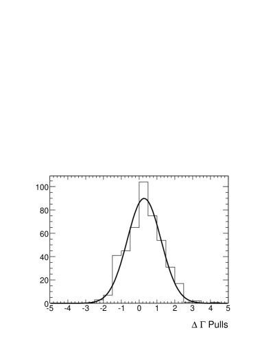
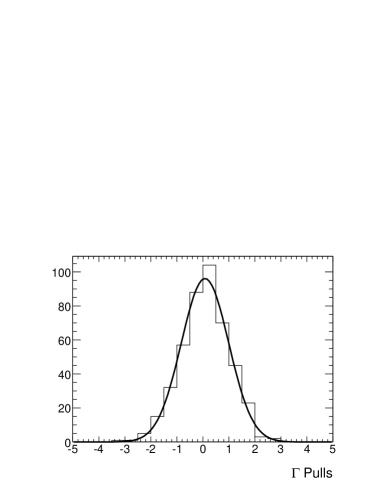
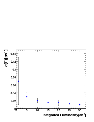
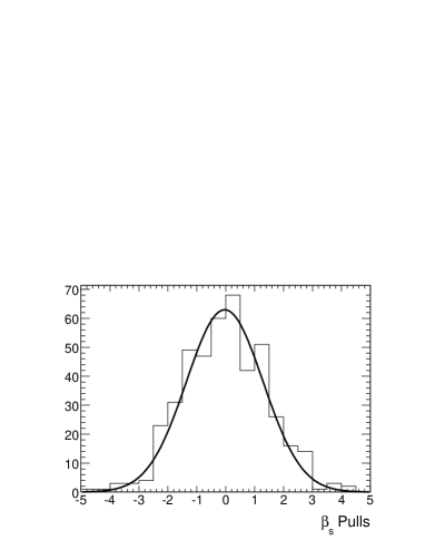
Figure 11: Distributions of the pull for $\Delta\Gamma_{s}$ (top row), $\Gamma_{s}$ (middle row) and $\beta_{s}$ (bottom row) from a set of 900 toy Monte Carlo experiments, assuming an integrated luminosity of $30\,ab^{-1}$ (left) and the trend of the error as a function of the integrated luminosity (right). The error bars, in the right plots, show the RMS of the error distribution.

5.3.2 Charge asymmetry in semileptonic decays

The amplitude describing $B_{s}$–$\bar{B}_{s}$ mixing can be experimentally constrained looking at the difference between the $B_{s}$ and $\bar{B}_{s}$ semileptonic decay rates after the mixing of the $B_{s}$ mesons. Since the charge of the lepton tags the flavour of the $B_{s}$ meson at the decay point, and since the decay amplitude is characterized by only one combination of CKM elements, any deviation of the charge asymmetry from zero can only come from a deviation of $|q/p|$ from one. One can define the semileptonic asymmetry as :

$$A_{SL}^{s}=\frac{BR(B_{s}\rightarrow\bar{B}_{s}\rightarrow D_{s}^{(*)-}{\it l}^{+}\nu_{\it l})-BR(\bar{B}_{s}\rightarrow B_{s}\rightarrow D_{s}^{(*)+}{\it l}^{-}\nu_{\it l})}{BR(B_{s}\rightarrow\bar{B}_{s}\rightarrow D_{s}^{(*)-}{\it l}^{+}\nu_{\it l})+BR(\bar{B}_{s}\rightarrow B_{s}\rightarrow D_{s}^{(*)+}{\it l}^{-}\nu_{\it l})}=\frac{1-|q/p|^{4}}{1+|q/p|^{4}}.$$ (13)

To measure $A_{SL}^{s}$, we exclusively reconstruct one of the two $B$ mesons into a self-tagging hadronic final state (such as $B_{s}\rightarrow D_{s}^{(*)}\pi$) and look for the signature of a semileptonic decay (high momentum lepton) in the rest of the event (ROE). Since both the $B$ mesons are reconstructed from self-tagging modes, it is possible to isolate those events in which the two $B_{s}$ mesons have the same flavour content. To increase the statistics, one can also avoid to reconstruct one of the two $B$ mesons and determine its flavour on a probabilistic basis, using a tagging algorithm.

To evaluate the expected error associated to this strategy, we use a toy Monte Carlo technique, generating and fitting a large set of toy-simulated data samples. We use two variables to discriminate signal from background, namely the $m_{miss}^{s}$ of the fully reconstructed $B_{s}\rightarrow D_{s}^{(*)}\pi$ candidate, and the missing mass of the other $B$, $m_{\nu}$. Signal events peak in the region $m_{miss}^{s}\sim 5.46$ GeV and $m_{\nu}\sim 0$ GeV. We describe the event distributions using the function of Eq. (6) for $m_{miss}^{s}$ and the sum of four Gaussians for $m_{\nu}$. The continuum background, coming from the combinatoric of particles in the hadronization of $e^{+}e^{-}\rightarrow q\bar{q}$ events ($q=u,d,s,c$) ($\sim 10\%$ of the signal yield) is described by the phase-space threshold function of Eq. (7) for $m_{miss}^{s}$ and a second order polynomial for $m_{\nu}$. An additional source of background comes from other $B_{s}$ decays ($\sim 2.5\%$ of the signal yield), which can be described by the $m^{s}_{miss}$ PDF used for signal and an order one polynomial for $m_{\nu}$. Background from $\Upsilon(5S)\rightarrow BB\pi$ events is strongly suppressed, since both the $B$ mesons of the event are requested to decay into $D_{s}$ mesons, which occur through CKM suppressed amplitudes for $B_{d}$ and $B^{+}$ mesons.

We calculated the expected $q\bar{q}$ background yield scaling the values obtained by BaBar [48]. For signal, we consider both $D_{s}l\nu$ and $D^{*}l\nu$ events ($l=e,\mu$), assuming $BR(B_{s}\rightarrow D_{s}l\nu)=2\%$, $BR(B_{s}\rightarrow D_{s}^{*}l\nu)=4\%$, and the efficiency and purity of the BaBar analysis.

The result of the simulation is shown in Fig. 12, where the statistical error on $A_{SL}$ is given as a function of the integrated luminosity. The dashed line on the plot represents the current value of the systematic error typically quoted in precision measurements of direct CP asymmetries at the $B$-Factories. It is not unrealistic to expect an improvement of a factor two in the evaluation of the systematic error, considering that a sizable part of it has a statistical nature (being related to the available statistics for control samples).

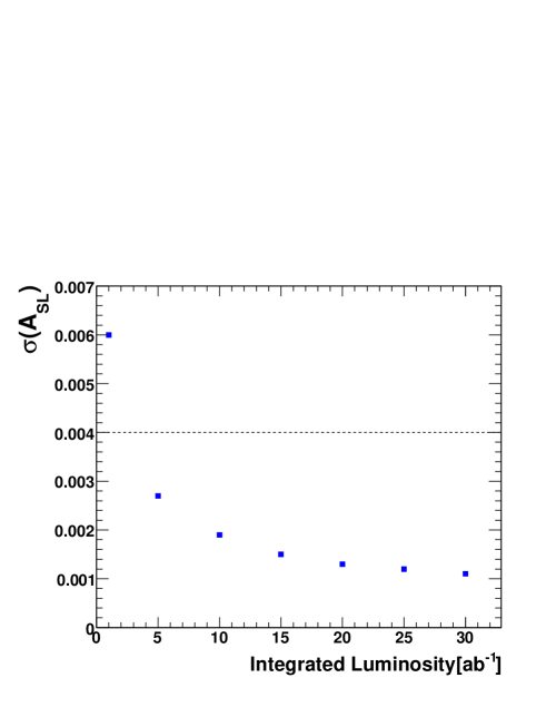
Figure 12: Statistical error on $A_{SL}^{s}$, as a function of the integrated luminosity. The dashed line represents the order of magnitude of the current systematic error on $A_{CP}$ measurements, shown for comparison.

5.3.3 Inclusive Measurement of Dimuon Charge Asymmetry

Running at the $\Upsilon(4S)$, the measurement of $A_{SL}^{d}$ can also be performed in an inclusive way, identifying $B\bar{B}$ events from pairs of same-sign leptons with positive ($N^{++}$) and negative ($N^{--}$) charge and calculating the charge asymmetry as

$$A_{SL}^{d} = \frac{N^{--}-N^{++}}{N^{--}+N^{++}}.$$ (14)

These events correspond to $\Upsilon(4S)$ decays in which both the $B$ mesons decay into a semileptonic final state. Requiring the charge of the leptons to be the same, is equivalent to select only events for which the two mesons have the same $b$ flavour content, which can happen only after a $B$–$\bar{B}$ mixing process. Contrary to the analysis presented in the previous section ($A_{SL}^{s}$), the cascade events component has to be controlled. A non-null value of $A_{SL}^{d}$ is sensitive to CP violating effects in the mixing process, i.e. to the weak phase of the mixing.

The situation of the $\Upsilon(5S)$ is more complicated: $B_{s}$ and $B_{d,u}$ mesons are produced simultaneously, but cannot be separated during the reconstruction, since the analysis is done inclusively. In this case, the measured observable can be written as

$$A_{CH} = \frac{N^{--}-N^{++}}{N^{--}+N^{++}}=\frac{\chi-\bar{\chi}}{\chi+\bar{\chi}-2\chi\bar{\chi}}$$ (15)

where $\chi=(1-f_{s})\chi_{d}+f_{s}\chi_{s}$, $\bar{\chi}=(1-f_{s})\bar{\chi}_{d}+f_{s}\bar{\chi}_{s}$, $f_{s}$ is the production rate of $B_{s}$ meson pairs at the $\Upsilon(5S)$ and

$$\stackrel{{\scriptstyle\scriptscriptstyle{(-)}}}{{\chi_{q}}}=\frac{\frac{\Delta\Gamma_{q}}{\Gamma_{q}}^{2}+4\frac{\Delta m_{q}}{\Gamma_{q}}^{2}}{\frac{\Delta\Gamma_{q}}{\Gamma_{q}}^{2}(\stackrel{{\scriptstyle\scriptscriptstyle{(-)}}}{{z_{q}}}-1)+4(2\stackrel{{\scriptstyle\scriptscriptstyle{(-)}}}{{z_{q}}}+\frac{\Delta m_{q}}{\Gamma_{q}}^{2}(1+\stackrel{{\scriptstyle\scriptscriptstyle{(-)}}}{{z_{q}}}))}~{}~{}~{}~{}~{}(q=d,s)$$ (16)

with $z_{q}=|q/p|_{q}^{2}$ and $\bar{z}_{q}=|p/q|_{q}^{2}$.

The interesting feature of this observable is that it relates NP effects in $B_{d}$ and $B_{s}$ sectors, providing an additional constraint with respect to the measurement of $A^{d,s}_{SL}$. The sample used for $A_{CH}$ can be orthogonal to the one used for $A_{SL}^{s}$ ($A_{SL}^{d}$) measurements if one avoids the use of semileptonic decays to reconstruct the other $B$ meson in the latter analysis.

From the experimental point of view, the main background sources are $q\bar{q}$ events ($q=u,d,s,c$) and cascade-lepton events in which one of the two leptons is generated from the semileptonic decay of a $D$ meson, coming from the $B$ decay. These backgrounds can be separated from signal looking at the distribution of the decay time [49]. The charge of the muon distinguishes $B$ and $\bar{B}$ mesons, while the information on the shape of the event in the CM frame allows to improve the rejection of $q\bar{q}$ background. The residual $B\bar{B}$ background, coming from cascade-lepton events can be suppressed using a Neural Network algorithm, based on:

• the momenta of the two leptons with the highest momentum in the $\Upsilon(5S)$ center of mass system;

• the total visible energy and the missing momentum of the event in the $\Upsilon(5S)$ center of mass system;

• the opening angle between the leptons in the $\Upsilon(5S)$ center of mass system;

and trained on simulated samples of signal and background events.

A rough estimate of the expected error achievable on the inclusive approach can be obtained scaling the statistical error quoted in the corresponding BaBar analysis [49] according to the inverse of $N_{S}/\sqrt{N_{S}+N_{B}}$, where $N_{S}$ and $N_{B}$ are the expected yields for signal and background respectively. The result, as a function of the luminosity, is given in Fig. 13. The dashed line represents the order of magnitude of the current systematic error on $A_{CP}$ measurement, shown for comparison. The measurement will be systematics dominated after a relatively small period of data taking, even though also in this case an improvement of the systematic error with an increased size of the control samples is possible. Notice that the information about $A_{SL}$ comes only from same sign events (i.e. with 2 leptons of the same sign), so only these events are taken into account in the error estimate.

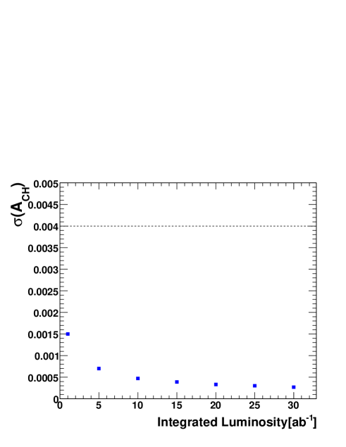
Figure 13: Statistical error on $A_{CH}$, as a function of the integrated luminosity. The dashed line represents the order of magnitude of systematic error on the current measurement at $\Upsilon(4S)$, shown for comparison.

6 Benchmark Measurements of $B_{s}$ rare decays

The production of $B_{s}$ mesons at the $\Upsilon(5S)$ allows to study the decay rates of the $B_{s}$ sector with the same completeness and accuracy that is currently available for the $B_{d}$ and charged $B$ mesons, improving our understanding of $B$ physics and helping to reduce the theoretical uncertainties related to NP-sensitive quantities. For instance, using the measurements of BR’s of $B_{s}$ mesons to open charm and to charmless decays it is possible to close the SU(3) multiplets of $b$ decays [50] and to control SU(3) breaking effects in channels like $B_{d}\rightarrow\phi K^{0}_{S}$ [51]. In addition, even without accessing time-dependent CP asymmetries, it is possible to access weak phases of $B_{s}$ decays. This is the case of the determination of $\gamma$ from the tree-level amplitudes of $B_{s}\rightarrow K\pi\pi^{0}$ decays, for which it is possible to disentangle penguin and tree contributions using the distribution of the events on the Dalitz plot [52].

On the other hand, $B_{s}$ physics provides a direct way to probe NP effects in the $b\rightarrow s$ transitions. Effects generated from NP particles are expected to be more evident in $b\rightarrow s$ than in $b\rightarrow d$ transitions, not only because, thanks to the CKM hierarchy among the amplitudes, the effect of hadronic uncertainties on the calculation of the SM is smaller than in the case of $b\rightarrow d$ processes, but also because this scenario is still allowed by the generalized UT analysis beyond the SM [32] and is expected in several extensions of the SM [53].

In the following we concentrate on this point. We show what could be learned from a high statistics study of $B_{s}$ mesons by giving some benchmark examples. In some cases, only at very high statistics and with particular detector performances, one can reach the same precision as at LHCb. Anyhow, one should take into account that the set of measurements we consider is not an exhaustive representation of the potential of a $B$-Factory running at the $\Upsilon(5S)$ and that a quantitative comparison between the performance of LHCb and a next-generation $B$-Factory, based on a common set of measurements, goes beyond the purpose of this paper. What we rather want to prove is that, contrary to what is usually claimed, all the interesting measurements (rates of rare decays, angular analyses, measurement of direct CP asymmetry and weak phases in $B_{s}$–$\bar{B}_{s}$ oscillations) can be performed even if $B_{s}$–$\bar{B}_{s}$ oscillation cannot be accessed. To demonstrate this point, we already documented in Sec. 5 how the $B_{s}$–$\bar{B}_{s}$ mixing phase $\beta_{s}$ can be measured in tree-level and in penguin modes, testing the SM in $B_{s}$–$\bar{B}_{s}$ mixing as well as in $b\rightarrow s$ transitions. In this section, we discuss two other milestones of a $B_{s}$ physics program, namely the measurement of the BR of rare decays of the $B_{s}$, and the test of the SM through the determination of $|V_{td}/V_{ts}|$ in penguin dominated modes.

The main result of this study is that a $B$-Factory running at the $\Upsilon(5S)$ will not be limited by detector performances. Using the analyses techniques we briefly describe here, it will be possible to study several decays which might go beyond the capability of LHCb, such as channels without primary tracks in the decay and/or channels with only photons in the final state. Furthermore, the possibility of studying channels with open kinematic (such as $b\rightarrow ul\nu$ and $b\rightarrow s\nu\bar{\nu}$), even with a factor three reduction in statistics with respect to the $\Upsilon(4S)$ represents something that only at a $B$-Factory can be determined. In our opinion, the sum of all these arguments establishes the complementarity between the physics program of LHCb and the possibility of studying $B$ mesons at the $\Upsilon(5S)$. So, while LHCb will provide high precision measurements for a limited set of observables, a B factory running at the $\Upsilon(5S)$ will be able to acccess (not nececssarely with a comparable precision) a much larger ensamble of quantities. If this is done before the LHCb will start collecting data, already with two ab^-1 it will be possible to exclude NP contributions comparable to the SM amplitude, as well as to provide a set of measurements of rates and asymmetries to be used by LHCb as a calibration of the physics measurements in the very first run period.

6.1 Probing New Physics in penguins with $|V_{td}/V_{ts}|$

The measurement of $\Delta m_{s}$ at the Tevatron [10] has provided a further evidence of the consistency between experimental data and the predictions of the SM. The agreement between the prediction by UTfit [54] and the measured value of $|V_{td}/V_{ts}|$ has reduced the possibility of observing large NP effects in $B_{s}$–$\bar{B}_{s}$ oscillations [32]. Nevertheless, it is still interesting to probe NP in $b\rightarrow s$ channels using an independent determination of $|V_{td}/V_{ts}|$, which might be sensitive to NP in a different way than $\Delta m_{s}$. It has been proposed in literature that such a test can be provided by the ratio $R=BR(B^{0}\rightarrow\rho^{0}\gamma)/BR(B\rightarrow K^{*0}\gamma)$ [55]. This quantity can be expressed as

$$R\equiv c_{\rho}^{2}\frac{r_{m}}{\xi^{2}}\frac{|a_{7}^{c}(\rho\gamma)|^{2}}{|a_{7}^{c}(K^{*0}\gamma)|^{2}}\frac{|V_{td}|^{2}}{|V_{ts}|^{2}}(1+\Delta R)$$ (17)

where $\frac{|V_{td}|}{|V_{ts}|}$ is the combination of CKM elements one wants to determine; $\frac{|a_{7}^{c}(\rho\gamma)|^{2}}{|a_{7}^{c}(K^{*0}\gamma)|^{\prime\prime}}$ is the difference in the penguin factorized decay amplitude, due to the different mesons in the final state; $r_{m}$ is defined as $r_{m}=(\frac{m_{B}^{2}-m_{\rho}^{2}}{m_{B}^{2}-m_{K^{*0}}^{2}})^{3}$; $\xi$ is the ratio of form factors $F(B\rightarrow K^{*0})/F(B\rightarrow\rho)$, and $\Delta R$ is a correction generated by the annihilation contribution to $B\rightarrow\rho\gamma$ (see Fig. 14), which is not present in $B\rightarrow K^{*0}\gamma$.

Figure 14: Annihilation contribution to the $b\rightarrow d$ amplitude of $B\rightarrow\rho\gamma$ decays.

This ratio provides an independent test of the SM prediction of $|V_{td}/V_{ts}|$, since radiative decays are particularly sensitive to NP contributions. As these processes violate chirality, the decay amplitude in the SM is proportional to $m_{q}$, the mass of the quark ($q=b,s$) generating the helicity flip. In presence of NP, the helicity flip is obtained by the mass insertion of a new heavy state, determining the enhancement of the NP amplitude with respect to the SM by a factor $m_{HS}/m_{q}$, where $m_{HS}$ is the mass of the new heavy state. This implies that it is possible to observe NP effects in these channels even when the contribution is too small to be determined in the $B$–$\bar{B}$ mixing.

A limitation to the effectiveness of this test comes from the presence of the $\Delta R$ term in Eq. (17). In the SM this contribution is not only expected to be $\mathcal{O}(\Lambda_{QCD}/m_{b})$ but it is also CKM suppressed, being proportional to $\cos(\alpha)$ [55]. These two suppressions reduce the sensitivity to non perturbative QCD effects that determines the value of $\Delta R$. The main limitation is related to the fact that, beyond the SM, the CKM factor is not necessarily small. While in MFV models the $\cos(\alpha)$ suppression still reduces the sensitivity to the hadronic corrections, this is not the case for models with a generic flavour structure. This is why it is particularly interesting to look for a similar observable which is not affected by the presence of the annihilation term.

Such observable can be provided by the ratio $R=BR(B_{s}^{0}\rightarrow K^{*0}\gamma)/BR(B_{d}\rightarrow K^{*0}\gamma)$. In this case, in fact, the two decays are not affected by annihilation contributions and the ratio is governed by Eq. (17), with $\frac{|a_{7}^{c}(\rho\gamma)|}{|a_{7}^{c}(K^{*0}\gamma)|}$ and $\xi$ replaced by the similar factors, and where the $\Delta R$ term vanishes.

The BR measurement for $B_{d}\rightarrow K^{*0}\gamma$ has been performed at the current $B$-Factories [56] and the present error is (almost) dominated by the systematic error. We assume $BR(B_{d}\rightarrow K^{*0}\gamma)=(40.1\pm 2.4)\cdot 10^{-6}$, corresponding to the current world average, with the error given by the current systematic error.

An estimate of the error that can be obtained for $BR(B_{s}^{0}\rightarrow K^{*0}\gamma)$ has been extracted performing toy Monte Carlo simulations as a function of the integrated luminosity. The SM expectation value for $BR(B_{s}^{0}\rightarrow K^{*0}\gamma)$ is about two times its $B_{d}$ counterparts, $B_{d}^{0}\rightarrow\rho^{0}\gamma$. As a reference, we use $BR(B_{s}^{0}\rightarrow K^{*0}\gamma)=1.8\cdot 10^{-6}$, obtained using the central value of the current world average for $B_{d}^{0}\rightarrow\rho^{0}\gamma$ [57] and the relative factor two, coming from the Clebsch-Gordon coefficient of the $\rho^{0}$.

The distribution of the relative errors on the BR from the toy experiments as a function of the integrated luminosity is shown in the left plot of Fig. 15. The information coming from the toy experiments, combined to the current predictions on $\xi$ ($\xi=1.17\pm 0.09$ [58]), allows to determined the value of $\frac{|V_{td}|}{|V_{ts}|}$. The result is shown in the right plot of Fig. 15. By repeating the exercise after reducing the error on $\xi$, we verified that the determination of $\frac{|V_{td}|}{|V_{ts}|}$ is dominated by the statistical error even for large values of integrated luminosity.

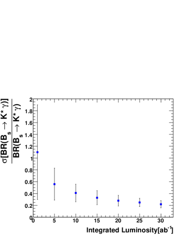
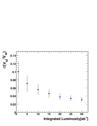
Figure 15: Distribution of the statistical error on $BR(B_{s}^{0}\rightarrow K^{*0}\gamma)$ from toy Monte Carlo experiments (left) and the expected error of the $|V_{td}/V_{ts}|$ measurement (right), as a function of the integrated luminosity.

6.2 $B_{s}\rightarrow\mu\mu$ and the flavour structure of New Physics

This decay plays a crucial role in study the structure of the Higgs sector and assessing the value of $\tan\beta$. In the SM, the BR of this process is written as [59]

$$Br(B_{s}\rightarrow l^{+}l^{-})=\tau(B_{s})\frac{G^{2}_{\rm F}}{\pi}\left(\frac{\alpha}{4\pi\sin^{2}\theta_{w}}\right)^{2}f^{2}_{B_{s}}m^{2}_{l}m_{B_{s}}\sqrt{1-4\frac{m^{2}_{l}}{m^{2}_{B_{s}}}}|V^{\ast}_{tb}V_{ts}|^{2}Y^{2}(x_{t}),$$ (18)

where $x_{t}=m_{t}^{2}/m_{W}^{2}$, $f_{B_{s}}$ is the $B_{s}$ meson decay constant and, within the SM, $Y(x_{t})$ is the Inami-Lim function [60], given by the expression

$$Y(x_{t})={{x_{t}}\over 8}\;\left[{{x_{t}-4}\over{x_{t}-1}}+{{3x_{t}}\over{(x_{t}-1)^{2}}}\ln x_{t}\right].$$ (19)

The SM expectation for this decay rate is $BR(B_{s}\rightarrow\mu\mu)=(3.35\pm 0.32)\cdot 10^{-9}$ [61]. The decay occurs in the SM through loop diagrams, which make this process particularly sensitive to NP contributions. For instance, the observation of this decay above the SM prediction will provide a clear evidence of new heavy states contributing to virtual processes. Recently, a combined analysis of $B$ and $K$ rare decays [62] has addressed this point in a quantitative way in the context of MFV models at small $\tan\beta$, obtaining $BR(B_{s}\rightarrow\mu\mu)<7.4\cdot 10^{-9}$ at $95\%$ probability. This result indicates that in MFV at small $\tan\beta$ we do not expect a large enhancement of the decay rate. Conversely, in very large $\tan\beta$ scenarios [63], $\tan\beta$–enhanced terms can still give sizable contributions resulting in a enhancement of the decay rate well beyond the above limit.

In order to estimate the expected experimental sensitivity in the SM, we assume the expectation value quoted above. We only consider $B_{s}$–$\bar{B}_{s}$ pairs from VV events. Since $BR(B_{d}\rightarrow\mu\mu)$ is suppressed by more than a factor of ten with respect to $BR(B_{s}\rightarrow\mu\mu)$, both in SM and in NP scenarios, we can neglect $B_{d}\bar{B}_{d}\pi$ events. The contamination coming from $B_{s}\rightarrow\pi\pi$ events is lower than in the case of $B_{d}$, since the decay is CKM suppressed. As for the search of $B_{d}\rightarrow\mu\mu$ performed by the $B$-Factories [64], the hadronic background can be suppressed imposing a set of requirements on PID, typically combined into a PID neural net. The cost is about a factor $60\%$ for the reconstruction efficiency. With respect to the $B$-Factories, we can also imagine a detector configuration with larger acceptance, thanks to a reduction of the Lorentz boost . Assuming a typical value of the reconstruction efficiency of $60\%$ we expect $6$ signal events and $960$ background events in $30$ ab^-1 of integrated data.

We use a set of toy Monte Carlo to evaluate the sensitivity of this measurement using $m_{miss}$, $\Delta E$ and the Fisher discriminant $\cal F$ as discriminating variables. We first generate signal and background events according to the shape of kinematic ($m_{miss}$ and $\Delta E$) and topological ($\cal F$) variables, as determined from fully simulated Monte Carlo samples. Signal events peak at a value of $m_{miss}\sim 5.46$ GeV and $\Delta E\sim-47$ MeV. Both distributions are described by Eq. (6). For background events we use the threshold function of Eq. (7) for $m_{miss}$ and a second order polynomial for $\Delta E$. For $\cal F$, we use a bifurcated Gaussian to parameterize the signal distribution and the sum of two Gaussians for the background.

For each generated datasets, we perform a ML fit as a function of the signal yield and obtain a shape of the likelihood for $N_{\mu\mu}$. We set the $90\%$ upper limit to the value $N_{UL}$ such that

$$\frac{\int_{0}^{N_{UL}}{\cal L}(N_{\mu\mu})dN_{\mu\mu}}{\int_{0}^{\infty}{\cal L}(N_{\mu\mu})dN_{\mu\mu}}=90\%.$$ (20)

We repeat this procedure for a large set of toys, as a function of the integrated luminosity. The result is shown in Fig. 16, where the full line represents the SM expectation and the errors bars the RMS of the upper limit distribution for each set of toy experiments. For comparison, the current $90\%$ C.L. experimental UL ($BR(B_{s}\rightarrow\mu^{+}\mu^{-})<8.0\cdot 10^{-8}$[65]) falls outside the range of the plot.

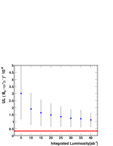
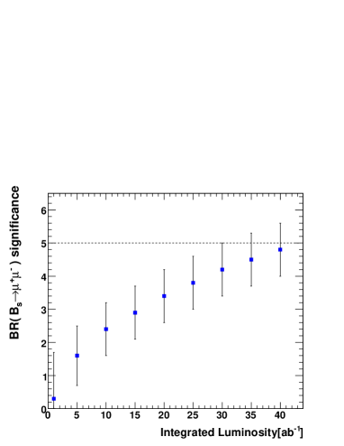
Figure 16: Distribution of the upper limit at $90\%$ C.L. (left) and statistical significance on the BR (right) for $BR(B_{s}\rightarrow\mu^{+}\mu^{-})$, as a function of the integrated luminosity. Error bars represent the RMS of the UL distribution for each set of toys. For the left (right) plot, the SM expectation for the BR (ten times the SM value) was assumed. On the right plot, the dashed line represent the $5\sigma$ evidence.

Since in several NP scenarios we expect a sizable contribution to the decay amplitude from new heavy states, we repeated the exercise assuming a decay rate one order of magnitude larger than the SM prediction. In this case, it should be possible to measure the BR with a meaningful statistical significance, rather than setting an upper limit. This is shown in Fig. 16, where the statistical significance is given as a function of the integrated luminosity.

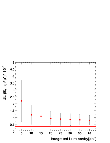
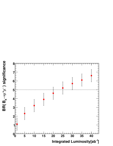
Figure 17: On the left upper limit distribution at $90\%$ C.L. for $BR(B_{s}\rightarrow\mu^{+}\mu^{-})$ in a Standard Model scenario, assuming a reduction of the background of a factor five as a function of the integrated luminosity. Error bars represent the RMS of the UL distribution for each set of toys. The horizontal band represents the Standard Model prediction. On the right significance of the measurement for $BR(B_{s}\rightarrow\mu^{+}\mu^{-})$ in a New Physics scenario with an order of magnitude enhancement with respect to the Standard Model assuming a reduction of the background of a factor five, as a function of the integrated luminosity. Error bars represent the RMS of the significance distribution for each set of toys. The dashed line represent the $5\sigma$ evidence.

As for the case of $B_{s}\rightarrow K^{0}\bar{K}^{0}$, discussed in Sec. 5.2.3, this channel is affected by a large background contamination from $q\bar{q}$ continuum events ($q=u,d,s,j$), which are characterized by a jet-like structure, with all the particles coming from the primary vertex. Considering the possibility of an upgrade of the vertexing detector with modern technologies, it is possible to use the improved vertexing resolution [43] to separate the $B$ and $D$ vertexes on the tag side for signal events and reject $q\bar{q}$ events, for which no secondary vertex is present. Using this additional requirement, it could be possible to strongly reduce the continuum background, improving the experimental precision. To give an idea of the impact of this improvement on the search of rare decays, we repeated the previous exercise assuming a reduction of continuum background by a factor of five, which might not represent an optimistic expectation. We show in Fig. 17 the impact of this improvement on the result of our toy studies, for both the SM and the enhanced values of the BR considered above. In this case, one can obtain an observation of the BR in the enhanced scenario with a relatively small amount of statistics for a $10^{36}$cm^-2sec^-1 super $B$-Factory.
It is clear that in this case LHCb can perform much better, given the larger amount of $B_{s}$ produced in its environment and the clear signature of the muon tracks. In fact, LHCb is expected to be able to exclude the SM branching ratio already with 0.5 $fb^{-1}$ of collected data [39] and to reach $3\sigma$ and $5\sigma$ evidence of the SM signal respectively with 2 $fb^{-1}$ (one year) and of integrated luminosity. Moreover, also ATLAS and CMS experiments are expected to give $4\sigma$ signal after one year of nominal data taking at the luminosity of $\mathcal{L}=10^{34}$cm^-2sec^-1.

6.3 Measurement of $B_{s}\rightarrow\gamma\gamma$

For several years, $b\rightarrow s\gamma$ has been considered as the golden mode to probe NP in the flavour sector. From an experimental point of view, any attempt to study this transition has to face the fact that the present error on $BR(b\rightarrow s\gamma)$ is dominated by systematic effects. It is then interesting to look for other channels that can play a similar rôle in constraining NP, but do not imply the experimental complexities that are introduced in $b\rightarrow s\gamma$ by the knowledge of the photon spectrum. In this context, an interesting candidate is provided by $B_{s}\rightarrow\gamma\gamma$ decays. The final state contains CP-odd and CP-even states, allowing to study CP violating effects with the tagging algorithms usually adopted at $B$-Factories. The SM expectation for the BR is $BR(B_{s}\rightarrow\gamma\gamma)=2-8\cdot 10^{-7}$[67]. NP effects are expected to give sizable contributions to the decay rate in some particular scenarios. For instance, in R-parity violating SUSY models, neutralino exchange can enhance the decay rate up to $BR(B_{s}\rightarrow\gamma\gamma)\simeq 5\cdot 10^{-6}$[68]. On the other hand, in R-parity conserving SUSY models $BR(B_{s}\rightarrow\gamma\gamma)$ is found to be highly correlated with $BR(b\rightarrow s\gamma)$[69]. In fact, thanks to an extension of the Low theorem[70], the $b\rightarrow s\gamma\gamma$ operator can be expanded at $O(G_{f})$ on the standard operator basis needed for $b\rightarrow s\gamma$. Doing so, one can relate deviations from SM in $b\rightarrow s\gamma$ and $B_{s}\rightarrow\gamma\gamma$ processes, provided the fact that NP effects appear only in the matching of Wilson coefficients of the standard basis of operators of the $b\rightarrow s\gamma$ effective Hamiltonian.

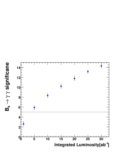
Figure 18: Statistical significance of the measurement of $BR(B_{s}\rightarrow\gamma\gamma)$ as a function of the integrated luminosity. Error bars represent the RMS of the significance distribution for each set of toys.

As already mentioned, the knowledge of the photon spectrum will always be a limiting factor for the measurement of $b\rightarrow s\gamma$ decay rate, whose error is presently systematically dominated and it is not expected to improve in the near future. On the other hand, the exclusive measurement of $B_{s}\rightarrow\gamma\gamma$ decay is very similar to other measurements already performed at $B$-Factories (such as $B^{0}\rightarrow\pi^{0}\pi^{0}$) and it is not affected by a theoretical error associated to the measurement (unlike the case of $b\rightarrow s\gamma$ analyses). From an experimental point of view, the limiting systematic factor is represented by the knowledge of the efficiency for photon reconstruction, which can be reduced with dedicated studies on control samples with similar energy range for the photons. On the other hand, the presence of two hard photons represents a clear signature for signal events, in particular if studied with recoil techniques.

In order to estimate the expected experimental sensitivity, we assume the same technique and the same performance in terms of efficiency and background rejection of the current BaBar search of $B_{d}\rightarrow\gamma\gamma$ [71]. The main source of background comes from hard photons from $\pi^{0}$ or $\eta$ decays, which are rejected requiring the invariant mass to be not within $\pm 3\sigma$ of the nominal $\pi^{0}$ or $\eta$ mass. Other sources of background, as initial state radiation, are removed with cuts on topological variables. The efficiency on signal event is $10\%$ and we expect $14$ signal events and $20$ background events in a sample of $1$ab^-1 of integrated data. We perform a set of toy Monte Carlo experiments, using $m_{ES}$, $\Delta E$, and $L_{2}/L_{0}$ in a ML fit. The result in term of the integrated luminosity is shown in Fig. 18. Considering that the measurement at $1$ab^-1 has already a $5\sigma$ significance, we conclude that a super $B$-Factory will be able to precisely measure the BR even at low statistic. Moreover, one will achieve a $7\%$ statistical precision on the measurement at $30$ab^-1, with a systematic error that will be smaller   than $5\%$. The large amount of events available even with few ab^-1 of integrated data will allow to measure also $B_{s}\rightarrow\gamma\gamma$ CP asymmetry. This will be possible with good accuracy exploiting a tagging algorithm which determines whether the other $B_{s}$ meson in the event decayed as a $B_{s}$ or a $\bar{B}_{s}$ (flavour tag)[72].

7 The impact on flavour physics: A possible future scenario

In the previous sections we tried to give an idea of how rich is the set of physics measurements a $B$-Factory can perform while running at the $\Upsilon(5S)$. The processes described represent a minimum set of measurements demonstrating the possibility of accessing rates and weak phases of rare decays, i.e. the necessary ingredients to test the SM.

Even with the limited amount of measurements we discussed, a facility like the one we are considering will have an impact on the knowledge of the flavour sector of NP. This might be clear enough from the previous chapters. In this section we make it more evident, showing how the unitarity triangle (UT) analysis will benefit from it. In order to do that, we consider two different scenarios:

• a low-statistics case, assuming that after collecting $2~{}{\rm ab}^{-1}$ of data at the $\Upsilon(4S)$, (one of) the two existing $B$-Factories will move to the $\Upsilon(5S)$, collecting $1~{}{\rm ab}^{-1}$ before LHCb will produce the first physics results.

• a high-statistics case, in which a high luminosity $B$-Factory will collect $75~{}{\rm ab}^{-1}$ at the $\Upsilon(4S)$ and then $30~{}{\rm ab}^{-1}$ at the $\Upsilon(5S)$ [13].

The low-statistics (high-statistics) scenario corresponds approximatively to fall 2009 (2015-2020). Taking into account the different time scales of the two projections, we consider two different sets of theoretical inputs: while for the low-statistics case we use the current values of the determinations of $f_{B_{s}}\sqrt{B_{B_{s}}}$, $\xi$, and $\hat{B}_{K}$, in the high-statistics case we assume that the increase of computation power will bring down the error of lattice QCD (LQCD) calculations to the percent level, while no improvement on the theory is considered. Indeed, since a constant progress in the calculation techniques has characterized the recent history of LQCD calculations, we can consider the estimates of the future errors relatively conservative.

Observable	low-statistics	high-statistics
	Error at $2\ {\rm ab}^{-1}$	Error at $75\ {\rm ab}^{-1}$
$\left|V_{cb}\right|$ (exclusive)	$4\%$	$1.0\%$
$\left|V_{cb}\right|$ (inclusive)	$1\%$	$0.5\%$
$\left|V_{ub}\right|$ (exclusive)	$8\%$	$2.0\%$
$\left|V_{ub}\right|$ (inclusive)	$8\%$	$2.0\%$
$BR(B\rightarrow\tau\nu)$	$20\%$	$4\%$
$f_{B_{s}}\sqrt{B_{B_{s}}}$	$13\%$	$1\%$
$\xi-1$	$26\%$	$5\%$
$\hat{B}_{K}$	$5\%$ $10\%$	$1\%$
$\sin(2\beta)$ ($J/\psi\,K^{0}$)	0.018	0.005
$\gamma$ ($B\rightarrow DK$, combined)	$\sim 6^{\circ}$	$1^{\circ}$
$\alpha$ (combined)	$\sim 6^{\circ}$	$1^{\circ}$
$2\beta+\gamma$ ($D^{(*)\pm}\pi^{\mp}$, $D^{\pm}K_{S}\pi^{\mp}$)	$20^{\circ}$	$5^{\circ}$

Table 3: Summary of the expected precision on the inputs of the UT analysis, in the low-statistics and high-statistics scenarios. The central values are taken in order to provide a perfect agreement among the constraints in the total fit.

In Tab. 3, we quote the errors on the experimental and theoretical inputs currently used in the UT analysis, based on measurements performed at the $\Upsilon(4S)$, together with $\epsilon_{K}$ from $K$–$\bar{K}$ mixing and $\Delta m_{s}$ from $B_{s}$–$\bar{B}_{s}$ mixing. In Tab. 4 we give the errors on the measurements performed at the $\Upsilon(5S)$, taken from the study presented in this paper. As mentioned in Sec. 5.2.2, we took into account an increase of the error of $\beta_{s}$ from $J/\psi\phi$ with tagged rates at positive and negative $\Delta t$, due to the presence of a two-fold ambiguity around $\beta_{s}\sim 0$.

7.1 The Unitarity Triangle in the Standard Model

We show in Fig. 19 how the SM analysis of the UT will look like in the two scenarios described above. The two plots correspond to an overall error of $\sigma_{\bar{\rho}}=9\%$ ($\sigma_{\bar{\eta}}=4\%$) on $\bar{\rho}$ ($\bar{\eta}$) for the low-statistics scenario and to an overall error $\sigma_{\bar{\rho}}=1.4\%$ ($\sigma_{\bar{\eta}}=0.8\%$) on $\bar{\rho}$ ($\bar{\eta}$) for the high-statistics one. For comparison, the current knowledge of the UT triangle gives $\sigma_{\bar{\rho}}=17\%$ and $\sigma_{\bar{\eta}}=5\%$.

Observable	low-statistics	high-statistics
	Error at $1\ {\rm ab}^{-1}$	Error at $30\ {\rm ab}^{-1}$
$\Delta\Gamma$	0.16 ps-1	0.03 ps-1
$\Gamma$	0.07 ps-1	0.01 ps-1
$\beta_{s}$ from angular analysis	$20^{\circ}$	$8^{\circ}$
$A^{s}_{SL}$	0.006	0.004
$A_{CH}$	0.004	0.004
$\beta_{s}$ from $J/\psi\phi$ $\Delta t$ sign	10∘	3∘
$V_{td}/V_{ts}$	0.10	0.031
$BR(B_{s}\rightarrow\mu^{+}\mu^{-})\cdot 10^{-8}$	$<$10 at 90$\%$ prob.	$<$ 1.30 at 90$\%$ prob.
$BR(B_{s}\rightarrow\gamma\gamma)$	38$\%$	7$\%$

Table 4: Expected errors for different observables considering an integrated luminosity of 1ab^-1 and 30ab^-1.

7.2 The Unitarity Triangle beyond the Standard Model

In a generic NP scenario the effect of $\Delta F=2$ NP contributions in $B_{q}$–$\bar{B}_{q}$ mixing can be parameterized in terms of two quantities, $C_{B_{q}}$ and $\phi_{B_{q}}$, which relate the experimental observables to the SM quantities. They are defined as [73]:

$$C_{B_{q}}\,e^{2i\phi_{B_{q}}}=\frac{\langle B_{q}|H_{\mathrm{eff}}^{\mathrm{full}}|\bar{B}_{q}\rangle}{\langle B_{q}|H_{\mathrm{eff}}^{\mathrm{SM}}|\bar{B}_{q}\rangle}=$$

$$=\frac{A_{q}^{\mathrm{SM}}e^{2i\phi_{q}^{\mathrm{SM}}}+A_{q}^{\mathrm{NP}}e^{2i(\phi_{q}^{\mathrm{SM}}+\phi_{q}^{\mathrm{NP}})}}{A_{q}^{\mathrm{SM}}e^{2i\phi_{q}^{\mathrm{SM}}}}\,,$$ (21)

where $H_{\mathrm{eff}}^{\mathrm{SM}}$ is the effective Hamiltonian, $H_{\mathrm{eff}}^{\mathrm{full}}$ is the Hamiltonian also including NP contributions, and $A_{q}^{\mathrm{SM}}e^{2i\phi_{q}^{\mathrm{SM}}}$ ($A_{q}^{\mathrm{NP}}e^{2i(\phi_{q}^{\mathrm{SM}}+\phi_{q}^{\mathrm{NP}})}$) is the SM (NP) amplitude. The two parameters $C_{B_{q}}$ and $\phi_{B_{q}}$ introduced in Eq. (21) allow to relate the SM value of a certain observable to its measured value. For instance, the measured values of the size and phase of $B_{d}$–$\bar{B}_{d}$ mixing are given by $\Delta m_{d}^{EXP}=C_{B_{d}}\Delta m_{d}^{SM}$ and $\beta^{EXP}=\beta+\phi_{B_{d}}$. Similar relations hold for the other observables of Tab. 3. Neglecting the case of NP contributions entering at tree-level processes, there are only two observables which do not depend on the presence of NP, namely $|V_{ub}/V_{cb}|$ and $\gamma$. 

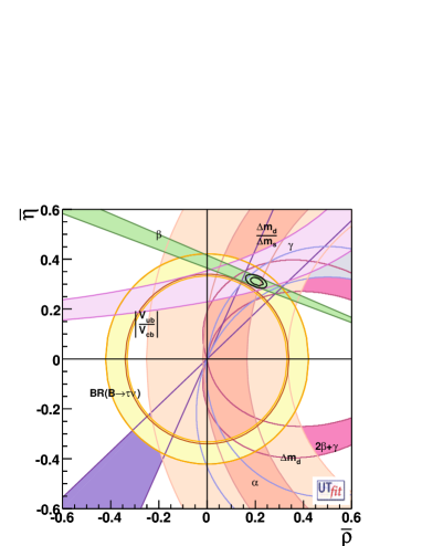
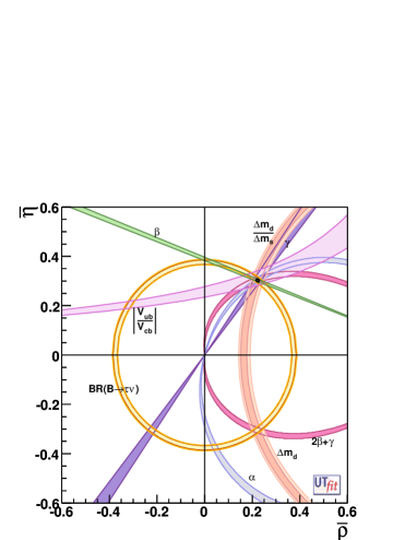
Figure 19: Determination of $\bar{\rho}$ and $\bar{\eta}$ in the Standard Model UT analysis for $2~{}{\rm ab}^{-1}$ (left) and $75~{}{\rm ab}^{-1}$ (right) projections of the errors as given in Tab. 3

Figure 20: Determination of $\bar{\rho}$ and $\bar{\eta}$ in the generalized UT analysis, obtained using all the available constraints for $2~{}{\rm ab}^{-1}$ (left) and $75~{}{\rm ab}^{-1}$ (right) projections of the errors as given in Tab. 3

Since under these assumptions we can parameterize NP effects just with two real parameters, without assuming any specific model, it is possible to determine the allowed region for NP, fitting simultaneously $C_{B_{d}}$, $\phi_{B_{d}}$, $\bar{\rho}$, and $\bar{\eta}$. Assuming the two scenarios of Tab. 3, we obtain the two plots given in Fig. 20 and the errors quoted in the first two raws of Tab. 5. The determination of $C_{B_{d}}$ and $\phi_{B_{d}}$ in the two cases is given in Fig. 21.

Parameter	low-statistics	high-statistics
	Error	Error
$\overline{\rho}$	$12\%$	$2.3\%$
$\overline{\eta}$	$8\%$	$1.8\%$
$C_{B_{d}}$	$0.43$	$0.032$
$\phi_{B_{d}}[^{\circ}]$	$1.7^{o}$	$0.44^{o}$
$C_{B_{s}}$	$0.33$	$0.026$
$\phi_{B_{s}}[^{\circ}]$	$7^{o}$	$1.9^{o}$

Table 5: Determination of UT and NP parameters from the generalized UT analysis, in the two scenarios of Tab. 3. For the $B_{s}$ sector, values from Tab. 4 are used.

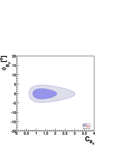
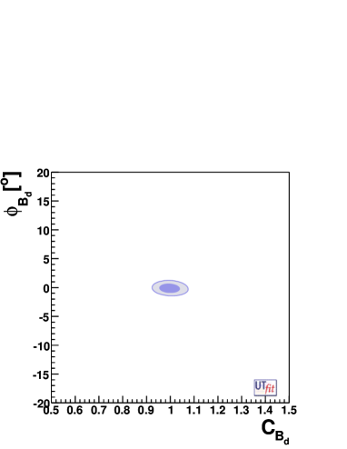
Figure 21: Determination of $C_{B_{d}}$ and $\phi_{B_{d}}$ in the generalized UT analysis for $2~{}{\rm ab}^{-1}$ (left) and $75~{}{\rm ab}^{-1}$ (right) projections of the errors given in Tab. 3, combined to the low-statistics (left) and high-statistics (right) scenarios of Tab. 4.

On top of this information, one can use the experimental information provided by the $\Upsilon(5S)$ run to constrain the values of $C_{B_{s}}$ and $\phi_{B_{s}}$. $C_{B_{s}}$ is directly related to the value of $\Delta m_{s}$, in analogy to the $B_{d}$ case, while $\phi_{B_{s}}$ is defined in such a way that $\beta_{s}^{EXP}=\beta_{s}-\phi_{B_{s}}$. The relation between the other constraints of Tab. 4 and the NP parameters is more complicated. It has been shown that the semileptonic CP asymmetry [45] and the value of $\Delta\Gamma_{s}/\Gamma_{s}$ [47] are sensitive to NP contributions to $\Delta F=2$ effective Hamiltonian. We use the NLO expression of these observables in terms of the parameters $C_{B_{s}}$ and $\phi_{B_{s}}$ [32].

The result of the combination of all these measurements is shown in the two plots of Fig. 22 and quantified in the bottom part of Tab. 5. On top of this analysis, one can further test the presence of NP using $\Delta F=1$ processes, as already discussed in Sec. 5.2.3, relating $\Delta F=1$ and $\Delta F=2$ NP effects by using a specific NP model (see for example [76]).

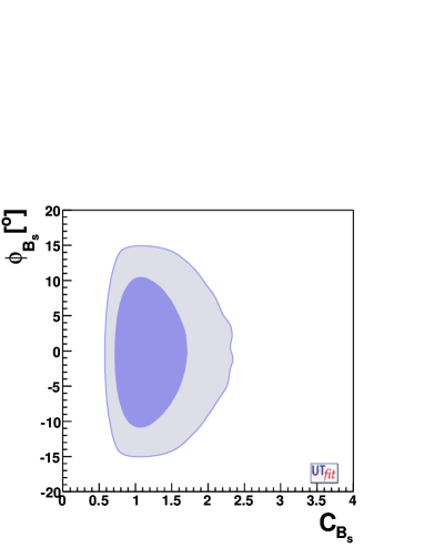
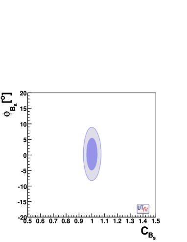
Figure 22: Determination of $C_{B_{s}}$ and $\phi_{B_{s}}$ in the generalized UT analysis for $1~{}{\rm ab}^{-1}$ (left) and $30~{}{\rm ab}^{-1}$ (right) projections of the errors for the input of Tab. 4. In the left (right) plot, $2~{}{\rm ab}^{-1}$ ($75~{}{\rm ab}^{-1}$) inputs of Tab. 3 are used for the other determinations.

7.3 A comparison with the reach of the LHCb experiment

Tab. 6 shows a comparison between the results presented in this paper and the expected sensitivity of LHCb for different benchmark measurement. The LHCb estimates are shown for an integrated luminosity of 2 $fb^{-1}$ (one year of nominal data taking) and 10 $fb^{-1}$ (full data taking), using the errors on lattice predictions expected on 2009 and 2015 respectively. The two scenarios described in the previous sections are used for a $B$-Factory running at the $\Upsilon(5S)$ resonance. The measurement of $\Delta m_{s}$ at LHCb is supposed to be dominated by a systematic error of 0.09 $ps^{-1}$ [39]. The relative error on $B_{d}\rightarrow K^{*0}\gamma$ is estimated to be $\sim$ 5% (dominated by the systematics on the branching ratio’s normalization). The relative error on $B_{s}\rightarrow K^{*0}\gamma$ is estimated to be $\sim$ 20% in the 2 $fb^{-1}$ scenario and $\sim$ 10% in the 10 $fb^{-1}$ scenario [77, 78]. In the $A^{s}_{SL}$ and $A_{CH}$ measurements both statistical and systematic uncertainties are shown.

In doing this comparison, the reader should remember that a reliable estimate of important systematic effects is not available for several LHCb measurements, while these uncertainties are typically well known and under control at the $B$-Factories. Moreover, we want to stress here that we presented only a minimal subsample of the possible measurements that can be performed at a $B$-Factory running at the $\Upsilon(5S)$, aiming to demonstrate the experimental feasibility of the corresponding analysis techniques. In the channels we chose, our estimates are mostly not competitive with respect to LHCb, but through them we proved the possibility to widely apply these techniques, in order to investigate several channels that cannot be studied in the LHC environment.

	LHCb		$\Upsilon(5S)$
Observable	$2fb^{-1}$	$10fb^{-1}$	$1ab^{-1}$	$30ab^{-1}$
$|V_{td}/V_{ts}|$ from $\Delta m_{s}$	$0.010$	$0.002$	-	-
$\Delta\Gamma/\Gamma$	0.0092	0.004	0.12	0.02
$\beta_{s}$ from angular analysis	$0.66^{\circ}$	$0.29^{\circ}$	$20^{\circ}$	$8^{\circ}$
$A^{s}_{SL}$	-	-	$\pm 0.006\pm 0.004$	$\pm 0.001\pm 0.004$
$A_{CH}$	-	-	$\pm 0.0015\pm 0.004$	$\pm 0.0003\pm 0.004$
$\beta_{s}$ from $J/\psi\phi$ $\Delta t$ sign	-	-	$20^{\circ}$	$8^{\circ}$
$BR(B_{s}\rightarrow\mu\mu)$	$1.2\cdot 10^{-9}$	$0.7\cdot 10^{-9}$	$<10^{-7}$	$<1.30\cdot 10^{-8}$
$|V_{td}/V_{ts}|$ from radiative decays	0.03	0.015	0.10	0.031
$BR(B_{s}\rightarrow\gamma\gamma)$	-	-	38%	7%

Table 6: Expected errors for different observables at LHCb [39, 77, 78] and at a $B$-Factory running at the $\Upsilon(5S)$ resonance.

8 Conclusions

In this paper we discussed the physics potential of a $B$-Factory running at the $\Upsilon(5S)$. Assuming the performance of the detectors currently taking data at the two $B$-Factories, we proved that it is possible to obtain a pure sample of $B_{s}$ mesons and at the same time to cover the physics program of a traditional $B$-Factory. We discussed the detector limitations in studying $B_{s}$–$\bar{B}_{s}$ oscillations and we showed that, even if time-dependent measurements of $B_{s}$ are not accessible with the current vertex resolution, the same physics information can be obtained using time-integrated measurements. We also illustrated some benchmark analyses of rare $B_{s}$ decays, interesting to test the SM and obtain information on the flavour structure of the NP. With this limited set of examples, we proved that this facility can perform similar measurements using alternative techniques with respect to hadron collider experiments. On the other hand, thanks to the clean environment and the progress made by BaBar and Belle in the recent past, this facility allows to extend the LHCb physics program to a larger set of interesting channels which, not having prompt charged tracks and/or being characterized by the presence of photons in the final state, are difficult to study at a hadron collider. Examples of this kind are $B_{s}\rightarrow\gamma\gamma$ and $B_{s}\rightarrow K^{0}\bar{K}^{0}$. To conclude, we extrapolated the impact of the $B_{s}$ physics program on the unitarity triangle analysis beyond the standard model, considering the possibility of $1{\rm ab}^{-1}$ collected by the existing $B$-Factories after accumulating $2{\rm ab}^{-1}$ at the $\Upsilon(4S)$, or $30{\rm ab}^{-1}$ collected by a high luminosity $B$-Factory after collecting $75{\rm ab}^{-1}$ at the $\Upsilon(4S)$. We stress that the experimental precision on these observables is not necessarily better than what LHCb can achieve [79]. Nevertheless, this limited set of examples demonstrates that, even using different experimental techniques, the proposed machine can measure absolute values and (strong and weak) phases of decay amplitudes, even without directly accessing the time-dependent structure of $B_{s}$–$\bar{B}_{s}$ oscillation. Furthermore, thanks to the very clean environment, it is possible to apply the discussed experimental techniques to all $B$ decays, without any restriction related to the need of prompt tracks in the event. We do not cover all the examples of such additional potentiality with respect to hadron collider experiments, but only outline the cases of the measurements of the rate of $B_{s}\rightarrow\gamma\gamma$ decays and of the weak phase in $B_{s}\rightarrow K^{0}\bar{K}^{0}$ decays.

Concluding, we would like to stress that, unlike the case of $B_{d}$ and charged $B$ decays, the $B_{s}$ sector is presently largely unstudied. Based on what we discussed in this paper, we think that it is particularly interesting to consider the possibility of studying $B_{s}$ decays with BaBar and Belle before LHCb starts. This would maximize the physics impact of the luminosity that can be collected (less than $2$ab^-1), while a super $B$-Factory would be needed to obtain the required luminosity during and after LHC data taking.

9 Acknowledgments

We would like to thank G. Isidori and G. Martinelli for their help in writing Sec. 4.1, V. Lubicz for providing us the extrapolation of lattice QCD errors, R. Faccini for useful discussions and suggestions and for the feed-back provided during all the development of this work and E. Emili and D. Granata for their contribution in our early studies for this paper. We would also like to thank T. Browder and M. Hazumi for the interest shown for this work and for inviting us to take part at the BNMS2006 workshop series, which allowed us to compare our studies to the activity of the Belle community. This work has been supported in part by the France-Japon Particle Physics Laboratory FJ-PPL, the EU networks “The quest for unification” under the contract MRTN-CT-2004-503369, “FLAVIAnet” under the contract MRTN-CT-2006-035482, and “HEPTOOLS” under the contract MRTN-CT-2006-035505.

References

- [1] N. Cabibbo, Phys. Rev. Lett. 10 (1963) 531. M. Kobayashi and T. Maskawa, Prog. Theor. Phys. 49 (1973) 652.
- [2] B. Aubert et al. [BABAR Collaboration], Phys. Rev. Lett. 87 (2001) 091801 [arXiv:hep-ex/0107013]. K. Abe et al. [Belle Collaboration], Phys. Rev. Lett. 87 (2001) 091802 [arXiv:hep-ex/0107061]. B. Aubert et al. [BABAR Collaboration], arXiv:hep-ex/0607107. K. F. Chen et al. [Belle Collaboration], arXiv:hep-ex/0608039.
- [3] M. Ciuchini, E. Franco, G. Martinelli, L. Reina and L. Silvestrini, Z. Phys. C 68 (1995) 239 [arXiv:hep-ph/9501265].
- [4] P. Paganini, F. Parodi, P. Roudeau and A. Stocchi, Phys. Scripta 58 (1998) 556 [arXiv:hep-ph/9711261].
- [5] M. Bona et al. [UTfit Collaboration], JHEP 0610 (2006) 081 [arXiv:hep-ph/0606167]. Updated results are available on http://www.utfit.org. For a different approach, producing similar results, see J. Charles et al. [CKMfitter Group], Eur. Phys. J. C 41 (2005) 1 [arXiv:hep-ph/0406184].
- [6] B. Aubert et al. [BABAR Collaboration], Nucl. Instrum. Meth. A 479 (2002) 1 [arXiv:hep-ex/0105044].
- [7] A. Bondar et al. [BELLE Collaboration], Nucl. Instrum. Meth. A 408 (1998) 64.
- [8] F. Abe et al. [CDF Collaboration], Nucl. Instrum. Meth. A 271, (1988) 387. J. Cranshaw [CDF Collaboration], Nucl. Instrum. Meth. A 462, (2001) 170.
- [9] S. Abachi et al. [D Collaboration], Nucl. Instrum. Meth. A 338, (1994) 185. S. Abachi et al. [D Collaboration], Nucl. Instrum. Meth. A 408, (1998) 103.
- [10] V. M. Abazov et al. [D Collaboration], Phys. Rev. Lett. 97 (2006) 021802 [arXiv:hep-ex/0603029]. A. Abulencia [CDF - Run II Collaboration], Phys. Rev. Lett. 97 (2006) 062003 [arXiv:hep-ex/0606027].
- [11] O. Schneider et al. [LHCb Collaboration], Nucl. Instrum. Meth. A 446, 213 (2000).
- [12] B. Aubert et al. [BABAR Collaboration], Phys. Rev. D 71 (2005) 032005 [arXiv:hep-ex/0411016]. R. Itoh et al. [Belle Collaboration], Phys. Rev. Lett. 95 (2005) 091601 [arXiv:hep-ex/0504030].
- [13] M. Bona, “SuperB: A high-luminosity asymmetric e+ e- super flavor factory. Conceptual design report”, URL http://www.pi.infn.it/SuperB/?q=CDR.
- [14] W. M. W. Yao et al. [Particle Data Group], J. Phys. G 33 (2006) 1.
- [15] G. Huang et al. [CLEO Collaboration], arXiv:hep-ex/0607080.
- [16] D. Besson et al. [CLEO Collaboration], Phys. Rev. Lett. 54 (1985) 381. D. M. J. Lovelock et al., Phys. Rev. Lett. 54 (1985) 377.
- [17] A. Drutskoy, for Belle Collaboration arXiv:hep-ex/0605110.
- [18] See for example N. A. Tornqvist, Phys. Rev. Lett. 53 (1984) 878.
- [19] J. Ocariz et al., Babar Analysis Document
- [20] R. Fisher, Ann. Eugenics, vol. 7, pp. 179–188, 1936.
- [21] B. Aubert et al. [BABAR Collaboration], Phys. Rev. D 71 (2005) 111102 [arXiv:hep-ex/0503011].
- [22] See for example B. Aubert et al. [BABAR Collaboration], Phys. Rev. D 71 (2005) 091102 [arXiv:hep-ex/0502019].
- [23] S. J. Brodsky and J. R. Hiller, Phys. Rev. D 46 (1992) 2141.
- [24] F. Cardarelli, I. L. Grach, I. M. Narodetsky, G. Salme and S. Simula, Phys. Lett. B 349 (1995) 393 [arXiv:hep-ph/9502360]. D. Melikhov and S. Simula, Phys. Rev. D 65 (2002) 094043 [arXiv:hep-ph/0112044]. B. L. G. Bakker, H. M. G. Choi and C. R. G. Ji, Phys. Rev. D 67 (2003) 113007 [arXiv:hep-ph/0303002].
- [25] G. C. Branco, L. Lavoura, and J. P. Silva, “CP Violation”, Oxford University Press (1999).
- [26] M. Gronau and D. London, Phys. Rev. Lett. 65 (1990) 3381.
- [27] M. Bona et al. [UTfit Collaboration], arXiv:hep-ph/0701204.
- [28] B. Aubert et al. [BABAR Collaboration], arXiv:hep-ex/0607106.
- [29] P. Oddone, Annals N. Y. Acad. Sci. 578 (1989) 237.
- [30] B. Aubert et al. [BABAR Collaboration], arXiv:hep-ex/0203035.
- [31] B. Aubert et al. [BABAR Collaboration], Phys. Rev. D 66 (2002) 032003 [arXiv:hep-ex/0201020].
- [32] M. Bona et al. [UTfit Collaboration], JHEP 0603 (2006) 080 [arXiv:hep-ph/0509219]. M. Bona et al. [UTfit Collaboration], Phys. Rev. Lett. 97 (2006) 151803 [arXiv:hep-ph/0605213].
- [33] D. Acosta et al. [CDF Collaboration], Phys. Rev. Lett. 94 (2005) 101803 [arXiv:hep-ex/0412057].
- [34] H. Albrecht et al. [ARGUS Collaboration], Z. Phys. C 48 (1990) 543.
- [35] G. Batignani et al., contribution to the 15th International Workshop on Vertex Detectors (Verte06), available at the URL http://indico.cern.ch/materialDisplay.py?contribId=31&sessionId=10 &materialId=paper&confId=1151.
- [36] B. Aubert et al. [BABAR Collaboration], Phys. Rev. Lett. 93 (2004) 131805 [arXiv:hep-ex/0403001].
- [37] V. M. Abazov et al. [D Collaboration], arXiv:hep-ex/0701012.
- [38] S. Amato et al. [LHCb Collaboration], CERN-LHCC-98-4
- [39] M. H. Schune, talk given at the Super B Workshop Paris, May 9-11, 2007.
- [40] M. Ciuchini, M. Pierini and L. Silvestrini, Phys. Rev. Lett. 95 (2005) 221804 [arXiv:hep-ph/0507290].
- [41] M. Ciuchini, M. Pierini and L. Silvestrini, arXiv:hep-ph/0703137.
- [42] A. J. Buras and L. Silvestrini, Nucl. Phys. B 569 (2000) 3 [arXiv:hep-ph/9812392].
- [43] N. Neri and M.Pierini, study for the superB factory, presented at the first super B workshop, Frascati, Italy 11-12 November 2005
- [44] B. Aubert et al. [BABAR Collaboration], Phys. Rev. Lett. 97 (2006) 171805 [arXiv:hep-ex/0608036].
- [45] S. Laplace, Z. Ligeti, Y. Nir and G. Perez, Phys. Rev. D 65 (2002) 094040 [arXiv:hep-ph/0202010].
- [46] D. Acosta et al. [CDF Collaboration], “Analysis of decay-time dependence of angular distributions in and decays and measurement of the Phys. Rev. Lett. 94 (2005) 101803 [arXiv:hep-ex/0412057].
- [47] A. S. Dighe, I. Dunietz and R. Fleischer, Eur. Phys. J. C 6 (1999) 647 [arXiv:hep-ph/9804253]. I. Dunietz, R. Fleischer and U. Nierste, Phys. Rev. D 63 (2001) 114015 [arXiv:hep-ph/0012219].
- [48] B. Aubert et al. [BABAR Collaboration], arXiv:hep-ex/0607067.
- [49] B. Aubert et al. [BABAR Collaboration], Phys. Rev. Lett. 96 (2006) 251802 [arXiv:hep-ex/0603053].
- [50] B. Grinstein and R. F. Lebed, Phys. Rev. D 53 (1996) 6344 [arXiv:hep-ph/9602218].
- [51] Y. Grossman, Z. Ligeti, Y. Nir and H. Quinn, Phys. Rev. D 68 (2003) 015004 [arXiv:hep-ph/0303171].
- [52] M. Ciuchini, M. Pierini and L. Silvestrini, Phys. Lett. B 645 (2007) 201 [arXiv:hep-ph/0602207].
- [53] A. Pomarol and D. Tommasini, Nucl. Phys. B 466 (1996) 3 [arXiv:hep-ph/9507462]. R. Barbieri, G. R. Dvali and L. J. Hall, Phys. Lett. B 377 (1996) 76 [arXiv:hep-ph/9512388]. R. Barbieri, L. J. Hall and A. Romanino, Phys. Lett. B 401 (1997) 47 [arXiv:hep-ph/9702315].
- [54] M. Ciuchini et al., JHEP 0107 (2001) 013 [arXiv:hep-ph/0012308]. M. Bona et al. [UTfit Collaboration], JHEP 0507 (2005) 028 [arXiv:hep-ph/0501199].
- [55] M. Beneke, T. Feldmann and D. Seidel, Nucl. Phys. B 612 (2001) 25 [arXiv:hep-ph/0106067]. S. W. Bosch and G. Buchalla, Nucl. Phys. B 621 (2002) 459 [arXiv:hep-ph/0106081]. A. Ali, E. Lunghi and A. Y. Parkhomenko, Phys. Lett. B 595, (2004) 323 [arXiv:hep-ph/0405075]. S. W. Bosch and G. Buchalla, JHEP 0501 (2005) 035 [arXiv:hep-ph/0408231]. M. Beneke, T. Feldmann and D. Seidel, Eur. Phys. J. C 41 (2005) 173 [arXiv:hep-ph/0412400].
- [56] M. Nakao et al. [BELLE Collaboration], Phys. Rev. D 69 (2004) 112001 [arXiv:hep-ex/0402042]. B. Aubert et al. [BABAR Collaboration], Phys. Rev. D 70 (2004) 112006 [arXiv:hep-ex/0407003].
- [57] T. E. Coan et al. [CLEO Collaboration], Phys. Rev. Lett. 84 (2000) 5283 [arXiv:hep-ex/9912057]. K. Abe et al., Phys. Rev. Lett. 96 (2006) 221601 [arXiv:hep-ex/0506079]. B. Aubert [BABAR Collaboration], Phys. Rev. D 66 (2002) 010001 arXiv:hep-ex/0612017.
- [58] P. Ball and R. Zwicky, JHEP 0604 (2006) 046 [arXiv:hep-ph/0603232].
- [59] A. J. Buras, M. Spranger and A. Weiler, Nucl. Phys. B 660 (2003) 225 [arXiv:hep-ph/0212143].
- [60] T. Inami and C.S. Lim, Prog. Theor. Phys. 65 (1981) 297; ibid. 65 (1981) 1772.
- [61] M. Blanke, A. J. Buras, D. Guadagnoli and C. Tarantino, arXiv:hep-ph/0604057.
- [62] C. Bobeth, M. Bona, A. J. Buras, T. Ewerth, M. Pierini, L. Silvestrini and A. Weiler, Nucl. Phys. B 726 (2005) 252 [arXiv:hep-ph/0505110].
- [63] G. Isidori and A. Retico, JHEP 0111 (2001) 001 [arXiv:hep-ph/0110121].
- [64] T. Bergfeld et al. [CLEO Collaboration], Phys. Rev. D 62 (2000) 091102 [arXiv:hep-ex/0007042]. M. C. Chang et al. [BELLE Collaboration], Phys. Rev. D 68 (2003) 111101 [arXiv:hep-ex/0309069]. B. Aubert et al. [BABAR Collaboration], Phys. Rev. Lett. 94 (2005) 221803 [arXiv:hep-ex/0408096].
- [65] CDF Collaboration, note 8176.
- [66] M. Ciuchini, E. Franco, A. Masiero and L. Silvestrini, Phys. Rev. D 67 (2003) 075016 [Erratum-ibid. D 68 (2003) 079901] [arXiv:hep-ph/0212397].
- [67] L. Reina, G. Ricciardi and A. Soni, Phys. Rev. D 56 (1997) 5805 [arXiv:hep-ph/9706253].
- [68] A. Gemintern, S. Bar-Shalom and G. Eilam, Phys. Rev. D 70 (2004) 035008 [arXiv:hep-ph/0404152].
- [69] S. Bertolini and J. Matias, Phys. Rev. D 57 (1998) 4197 [arXiv:hep-ph/9709330].
- [70] G. L. Lin, J. Liu and Y. P. Yao, Phys. Rev. Lett. 64, 1498 (1990). G. L. Lin, J. Liu and Y. P. Yao, Phys. Rev. D 42 (1990) 2314.
- [71] B. Aubert et al. [BABAR Collaboration], Phys. Rev. Lett. 87 (2001) 241803 [arXiv:hep-ex/0107068].
- [72] B. Aubert et al. [BABAR Collaboration], Phys. Rev. Lett. 92 (2004) 201802 [arXiv:hep-ex/0312055].
- [73] J. M. Soares and L. Wolfenstein, Phys. Rev. D 47 (1993) 1021. N. G. Deshpande, B. Dutta and S. Oh, Phys. Rev. Lett. 77 (1996) 4499 [arXiv:hep-ph/9608231]. J. P. Silva and L. Wolfenstein, Phys. Rev. D 55 (1997) 5331 [arXiv:hep-ph/9610208]. A. G. Cohen, D. B. Kaplan, F. Lepeintre and A. E. Nelson, Phys. Rev. Lett. 78 (1997) 2300 [arXiv:hep-ph/9610252]. Y. Grossman, Y. Nir and M. P. Worah, Phys. Lett. B 407 (1997) 307 [arXiv:hep-ph/9704287].
- [74] A. Giri, Y. Grossman, A. Soffer and J. Zupan, Phys. Rev. D 68 (2003) 054018 [arXiv:hep-ph/0303187].
- [75] A. Amorim, M. G. Santos and J. P. Silva, Phys. Rev. D 59 (1999) 056001 [arXiv:hep-ph/9807364].
- [76] L. Silvestrini, arXiv:0705.1624 [hep-ph].
- [77] J. Dickens, talk given at the CKM 2006 Workshop, Nagoya, December 12-16, 2006.
- [78] V. Vagnoni, private communication.
- [79] O. Schneider, talk given at the LHCb Upgrade Workshop Edinburgh, January 11-12, 2006. Slides available at the URL http://lphe.epfl.ch/publications/2007/OSchneider_Edinburgh.ppt