Abstract

We use QCD sum rules to compute matrix elements of the $\Delta B=2$ operators appearing in the heavy-quark expansion of the width difference of the $B_{s}$ mass eigenstates. Our analysis includes the leading-order operators $Q$ and $Q_{S}$, as well as the subleading operators $R_{2}$ and $R_{3}$, which appear at next-to-leading order in the $1/m_{b}$ expansion. We conclude that the violation of the factorization approximation for these matrix elements due to non-perturbative vacuum condensates is as low as 1-2%.

1 Introduction

The phenomenon of flavour mixing has been intensively investigated over the last decades. The standard model of particle physics provides us with a parameterization of flavour physics which is compatible with all data taken up to now. However, we are still lacking a fundamental theory of flavour, explaining the three-family structure, the masses and mixings and CP violation.

The phenomenology of flavour mixing has a few peculiarities. In the standard model the only source of flavour mixing originates from the “mismatch” between the two mass matrices for the up and the down quarks, which is encoded in the relative rotation between the eigenbases of these matrices given by the CKM matrix. The mass matrices are induced by Yukawa couplings to the Higgs particle, which hints at a relation between electroweak symmetry breaking and the origin of flavour.

CP violation in the standard model is related to an irreducible phase in the CKM matrix, which can appear for at least three generations [1]. Putting aside the still unsolved mystery of strong CP violation [2], this leads to a few interesting conclusions which are confirmed by observation. One of these conclusions is the strong suppression of (CP violating) electric dipole moments of quarks and leptons, which is compatible with data. However, in a generic parameterization of “new physics” contributions it is hard to avoid electric dipole moments exceeding the experimental limits by orders of magnitude.

A further peculiarity of the standard parameterization of flavour physics is the suppression of “flavour changing neutral currents” (FCNC’s) by the GIM mechanism [3], which has its root in the unitarity of the CKM matrix. In particular, FCNC processes with $\Delta B=2$, $\Delta S=2$ have been intensively investigated, while $\Delta C=2$ processes have not yet been observed, in accordance with the very strong GIM suppression predicted by the standard model.

Especially in the systems of neutral $B$ mesons the theoretical description is simplified by the fact that the mass difference in these systems is dominated by the short distance contribution of the top quark. Furthermore, the width difference, which is expected to be sizable in the $B_{s}$ system, can be computed in the heavy-quark expansion [4].

The width difference $\Delta\Gamma$ between the $B_{s}$ mass eigenstates is determined by the off-diagonal matrix element $\Gamma_{12}$ of the $\Delta B=2$ transition operator ${\cal T}$ through $\Delta\Gamma=-2\Gamma_{12}$ where

$$\Gamma_{12}=\frac{1}{2M_{B_{s}}}\langle\bar{B}_{s}|{\cal T}|B_{s}\rangle$$ (1)

and $M_{B_{s}}$ is the $B_{s}$ meson mass. The $\Delta B=2$ transitions are initiated by a flavour changing neutral current and occur only at the loop level in the standard model. Therefore the transition operator ${\cal T}$ is a complicated, non-local object. The main problem however is the treatment of mesons as bound states of QCD, which involves dynamics in the infrared strong coupling regime, where a perturbative treatment is not possible. In the heavy-quark expansion the off-diagonal matrix element $\Gamma_{12}$ can be expanded as a series in inverse powers of the $b$-quark mass as

$$\langle\bar{B}_{s}|{\cal T}|B_{s}\rangle=\sum_{n}\frac{C_{n}}{m_{b}^{n}}\langle\bar{B}_{s}|{\cal O}_{n}^{\Delta B=2}|B_{s}\rangle$$ (2)

where the Wilson coefficients $C_{n}$ are calculable in perturbation theory [5]. In this formulation all the non-perturbative physics is contained in the matrix elements of the local $\Delta B=2$ operators ${\cal O}_{n}^{\Delta B=2}$. At leading order in $1/m_{b}$ the transition operator ${\cal T}$ involves two four-quark operators

$$Q = (\bar{b}_{i}s_{i})_{V-A}(\bar{b}_{j}s_{j})_{V-A}$$ (3)

$$Q_{S} = (\bar{b}_{i}s_{i})_{S-P}(\bar{b}_{j}s_{j})_{S-P}$$ (4)

with $i$ a color index. The notation is such that $(\bar{b}_{i}s_{i})_{V-A}=\bar{b}_{i}\gamma_{\mu}(1-\gamma_{5})s_{i}$ and $(\bar{b}_{i}s_{i})_{S-P}=\bar{b}_{i}(1-\gamma_{5})s_{i}$. At next-to-leading order in $1/m_{b}$ the transition operator involves five new (subleading) operators. The complete list of subleading operators and different choices of basis can be found in [6, 7]. We shall focus on the operators involving an extra covariant derivative acting on the strange-quark field, of which there are four. Neglecting higher-order terms in the $1/m_{b}$ expansion these can further be reduced to the two operators

$$R_{2} = \frac{1}{m_{b}^{2}}(\bar{b}_{i}{\overleftarrow{D}_{\mu}}{D}^{\mu}s_{i})_{V-A}(\bar{b}_{i}s_{i})_{V-A}$$ (5)

$$R_{3} = \frac{1}{m_{b}^{2}}(\bar{b}_{i}{{\overleftarrow{D}}}_{\mu}{D}^{\mu}s_{i})_{S-P}(\bar{b}_{i}s_{i})_{S-P}$$ (6)

with $D_{\mu}=\partial_{\mu}-ig_{s}A_{\mu}$ the covariant derivative. The subleading operators should be understood in HQET even though they are written formally in terms of full QCD fields. This means that the covariant derivative acting on the $b$-quark field in (5)-(6) can be replaced by $m_{b}v$ with $v$ the velocity of the heavy $b$-quark, making explicit that the subleading operators $R_{2}$ and $R_{3}$ are suppressed only by one power of $1/m_{b}$.

The standard parameterization of the matrix elements of these operators is obtained through the vacuum saturation approximation [8] with bag parameters $B_{i}$ controlling the accuracy of the factorization, $\langle\bar{B}_{s}|{\cal O}_{i}|B_{s}\rangle=B_{i}\langle\bar{B}_{s}|{\cal O}_{i}|B_{s}\rangle^{fac}$. For the operators considered here, we have (e.g. [6]) (we now use $B$ for the $B_{s}$ meson and also for the bag parameter of the operator $Q$)

$$\langle\bar{B}|Q|B\rangle = f_{B}^{2}M_{B}^{2}2\left(1+\frac{1}{N_{c}}\right)B$$ (7)

$$\langle\bar{B}|Q_{S}|B\rangle = -f_{B}^{2}M_{B}^{2}\frac{M_{B}^{2}}{(m_{b}+m_{s})^{2}}\left(2-\frac{1}{N_{c}}\right)B_{S}$$ (8)

$$\langle\bar{B}|R_{2}|B\rangle = -f_{B}^{2}M_{B}^{2}\left(\frac{M_{B}^{2}}{m_{b}^{2}}-1\right)\left(1-\frac{1}{N_{c}}\right)B_{2}$$ (9)

$$\langle\bar{B}|R_{3}|B\rangle = f_{B}^{2}M_{B}^{2}\left(\frac{M_{B}^{2}}{m_{b}^{2}}-1\right)\left(1+\frac{1}{2N_{c}}\right)B_{3},$$ (10)

where $N_{c}=3$ is the number of colors in QCD and $f_{B}$ is the $B_{s}$ meson semileptonic decay constant.

The dominant theoretical uncertainties in the prediction of $\Delta\Gamma=-2\Gamma_{12}$ using the heavy-quark expansion are related to the hadronic matrix elements of the local operators ${\cal O}_{i}\in\{Q,Q_{S},R_{2},R_{3}\}$, or equivalently, the bag parameters $B_{i}$. The calculation of the bag parameters involves strong interaction dynamics in the infrared region and is thus a problem in non-perturbative QCD. The ultimate solution can be provided by their direct calculation in lattice QCD. Results for $Q$ and $Q_{S}$ are available, although not yet completely reliable [9]. However, a computation for the operators $R_{2}$ and $R_{3}$ is completely lacking, and to match the increasing precision of the experimental data it is necessary to consider deviations from $B_{i}=1$ even for these subleading operators [7].

In this paper we use the technique of QCD sum rules to provide a first estimate of the bag parameters for the subleading operators $R_{2}$ and $R_{3}$. We focus on the calculation of the parameters $\Delta B_{i}=B_{i}-1$, which measure the deviations from the factorization result $B_{i}=1$. We limit our analysis to the non-perturbative vacuum condensate contributions to these quantities. While more sophisticated treatments with lattice QCD exist for the leading-order operators $Q$ and $Q_{S}$, and with QCD sum rules for $Q$, we also include these operators in our analysis. Studying the full set of operators simultaneously helps clarify the general features of sum rules as applied to this class of matrix elements.

Our main finding is that the non-perturbative contributions to $\Delta B$ are quite small for each of the four operators, no larger than 1-2%. We use a simple analytical analysis based on the HQET limit within finite energy sum rules (FESR) to give insight into this result. To explore corrections to the HQET limit and to provide error estimates we perform a more thorough numerical analysis using Borel sum rules. The numerical results suggest that corrections to the HQET limit may be large in some cases.

The paper is organized as follows. In Section 2 we describe the technique of sum rules as applied to our case and introduce some necessary notation. In Section 3 we describe the calculation of operator-product expansion (OPE) expressions for the Green functions used in the analysis. Sections 4 and 5 contain our sum-rule analysis and includes full QCD and the HQET limit in FESR and Borel form. In Section 6 we give the final results and discuss the assumptions made and uncertainties involved. In Section 7 we give the summary of the paper. Some long formulae for the OPE spectral densities are collected in the Appendix.

2 Sum rule calculation of the bag parameters:
the technique

In this section we review the sum-rule method for calculating the hadronic matrix elements of the $\Delta B=2$ operators. The starting point is the three-point correlator

$$T(p_{1},p_{2})=i^{2}\int d^{4}xd^{4}ye^{ip_{1}x-ip_{2}y}\langle Tj(x){\cal O}(0)j(y)\rangle.$$ (11)

The operator ${\cal O}\in\{Q,Q_{S},R_{2},R_{3}\}$ is a generic four-quark operator and the interpolating current $j$ for the $B$-meson can be either an axial-vector (AV) current or pseudoscalar (PS) current, defined as

$$j^{\mu}_{5} = \bar{s}\gamma^{\mu}\gamma_{5}b\qquad({\rm AV\,current})$$ (12)

$$j_{5} = \bar{s}i\gamma_{5}b\hskip 7.96674pt\qquad({\rm PS\,current}).$$ (13)

The overlap of the interpolating currents with $B$-meson states is defined through the matrix elements

$$\langle 0|\bar{s}\gamma_{\mu}\gamma_{5}b(0)|\bar{B}(p)\rangle=if_{B}p_{\mu},\qquad\langle 0|\bar{s}i\gamma_{5}b(0)|\bar{B}(p)\rangle=\frac{f_{B}M_{B}^{2}}{m_{b}+m_{s}},$$ (14)

where $f_{B}$ is the semileptonic decay constant of the $B$ meson, $M_{B}$ is the $B$-meson mass, $m_{b}$ is the $b$-quark mass, and $m_{s}$ is the strange-quark mass. For the axial-vector interpolating current the three-point correlator is a tensor, and we focus on the scalar function multiplying the tensor structure $p_{1}^{\mu}p_{2}^{\nu}$:

$$T^{\mu\nu}(p_{1},p_{2})=i^{2}\int d^{4}xd^{4}ye^{ip_{1}x-p_{2}y}\langle Tj^{\mu}_{5}(x){\cal O}(0)j^{\nu}_{5}(y)\rangle=p_{1}^{\mu}p_{2}^{\nu}T(p_{1},p_{2})+\ldots$$ (15)

where the ellipsis denote other tensor structures such as $p_{1}^{\mu}p_{1}^{\nu}$, $p_{2}^{\mu}p_{2}^{\nu}$, $p_{1}^{\nu}p_{2}^{\mu}$ or $g_{\mu\nu}$. It is convenient to use the dispersion relation

$$T(p_{1},p_{2})=\int ds_{1}ds_{2}\frac{\rho(s_{1},s_{2},q^{2})}{(s_{1}-p_{1}^{2})(s_{2}-p_{2}^{2})}$$ (16)

and work with the spectral density $\rho(s_{1},s_{2},q^{2})$. Here $q=p_{1}-p_{2}$ and $q^{2}=0$ at the physical point relevant to the mixing. To derive the sum rules the spectral density is evaluated in two ways:

1. In a phenomenological hadronic picture. In this case the spectral density is modeled by a $B$-meson pole plus a continuum contribution. This yields

   $$\rho^{\rm had}_{\rm AV}(s_{1},s_{2})=\left[f_{B}^{2}\delta(s_{1}-M_{B}^{2})\delta(s_{2}-M_{B}^{2})\langle\bar{B}|{\cal O}|B\rangle\right]+\rho^{\rm cont}_{\rm AV}$$ (17)

   for the axial-vector current, and

   $$\rho^{\rm had}_{\rm PS}(s_{1},s_{2})=\left[\frac{f_{B}^{2}M_{B}^{4}}{(m_{b}+m_{s})^{2}}\delta(s_{1}-M_{B}^{2})\delta(s_{2}-M_{B}^{2})\langle\bar{B}|{\cal O}|B\rangle\right]+\rho^{\rm cont}_{\rm PS}$$ (18)

   for the pseudoscalar current.

2. With QCD using the operator-product expansion. The resulting spectral densities $\rho^{\rm OPE}_{i}$ are the sum of a perturbative contribution and a non-perturbative contribution involving the vacuum matrix elements of local QCD operators (condensates).

The idea of QCD sum rules is to use duality between the physical spectrum measured in terms of hadrons and the OPE prediction expressed in terms of quarks and gluons (the degrees of freedom of the QCD Lagrangian). Duality is implemented by comparing integrals of the two spectral densities

$$\int ds_{1}ds_{2}\,\rho^{{\rm had}}_{i}(s_{1},s_{2})=\int ds_{1}ds_{2}\,\rho^{{\rm OPE}}_{i}(s_{1},s_{2}).$$ (19)

It is common practice to model the continuum contribution to the hadronic spectral density with the theoretical expression from the OPE. We choose to match the two expressions at the point $s_{1}=s_{2}=s_{0}$, so that the integration region $\Delta$ in the duality integral is the square $m_{b}^{2}<s_{i}<s_{0}$ in the $(s_{1},s_{2})$ plane. One then obtains the sum rules

$$f_{B}^{2}\langle\bar{B}|{\cal O}|B\rangle = \int_{\Delta}ds_{1}ds_{2}\,\rho^{\rm OPE}_{\rm AV}(s_{1},s_{2})\qquad({\rm AV\,current})$$ (20)

$$\frac{M_{B}^{4}}{(m_{b}+m_{s})^{2}}f_{B}^{2}\langle\bar{B}|{\cal O}|B\rangle = \int_{\Delta}ds_{1}ds_{2}\,\rho^{\rm OPE}_{\rm PS}(s_{1},s_{2})\qquad({\rm PS\,current}).$$ (21)

Calculating the OPE expressions for the spectral density thus allows for the extraction of the hadronic matrix elements $\langle\bar{B}|{\cal O}_{i}|B\rangle$, or, equivalently, the bag parameters $B_{i}$. The sum-rule results depend on the parameter $s_{0}$ at which the hadronic continuum is modeled by the OPE result; we shall discuss different ways of choosing this parameter later on.

The sum rules (20, 21) are referred to as “finite energy sum rules” (e.g. [10]). It is expected that results obtained with these basic sum rules give a reasonable approximation to a more sophisticated analysis. However, it is also useful to consider a different averaging procedure in the duality integrals. The most popular technique is the Borel sum rule analysis. In Borel sum rules one works with duality integrals of moments of the spectral densities rather than with the spectral densities themselves. In particular, one compares the derivatives $\partial^{n}/(\partial p^{2})^{n}$ of the spectral densities for large $n$. In the limit $n\to\infty$ and again modeling the hadronic continuum with the OPE prediction one arrives at the Borel sum rule

$$f_{B}^{2}\langle\bar{B}|{\cal O}|B\rangle e^{-\frac{M_{B}^{2}}{M^{2}_{1}}-\frac{M_{B}^{2}}{M^{2}_{2}}}=\int_{\Delta}ds_{1}ds_{2}\,e^{-\frac{s_{1}}{M^{2}_{1}}-\frac{s_{2}}{M^{2}_{2}}}\,\rho^{\rm OPE}_{\rm AV}(s_{1},s_{2})\qquad{(\rm AV\,current)}$$ (22)

and analogously for the pseudoscalar case. In the Borel sum rule contributions from excited states are exponentially suppressed. Also, studying the stability of the sum rule results under variations of the Borel parameters $M_{1}$ and $M_{2}$ helps assess their reliability.

The procedure sketched above can be used to compute the bag parameters directly. However, at the level of the OPE, one can identify the contributions to the three-point correlator which lead to the value $B=1$ only [11, 12]. Such contributions can be expressed as the product of two color-singlet two-point functions, each depending on a single momentum. Subtracting this trivial part from the QCD sum rule allows us to focus on the piece responsible for deviations from the factorized value. We thus split the three-point correlator into two pieces according to

$$T(p_{1},p_{2})=T_{\rm fac}(p_{1},p_{2})+\Delta T(p_{1},p_{2}),$$ (23)

where the sum rule obtained from the factorized piece $T_{\rm fac}$ yields $B=1$. This factorized part has the explicit form

$$T_{fac}(p_{1},p_{2})={\rm const}\times\Pi(p_{1})\Pi(p_{2})$$ (24)

with the “const” and the $\Pi(p_{i})$ specific to the operator involved. For instance, for the operators involving a V-A Dirac structure, one has

$$T_{fac}^{\rm AV}(p_{1},p_{2})=2\left(1+\frac{1}{N_{c}}\right)\Pi^{V}(p_{1})\Pi^{V}(p_{2})$$ (25)

with

$$p^{\alpha}\Pi^{V}(p)=i\int dxe^{ipx}\langle Tj(x)\bar{b}\gamma^{\alpha}(1-\gamma_{5})s(0)\rangle.$$ (26)

Using this same notation for the factorizable and non-factorizable contributions to the spectral densities one finds a sum rule for $\Delta B=B-1$ directly. It reads

$$f_{B}^{2}\Delta B\langle\bar{B}|{\cal O}|B\rangle^{fac}e^{-\frac{M_{B}^{2}}{M^{2}_{1}}-\frac{M_{B}^{2}}{M^{2}_{2}}}=\int ds_{1}ds_{2}\Delta\rho^{\rm OPE}_{\rm AV}(s_{1},s_{2})e^{-\frac{s_{1}}{M^{2}_{1}}-\frac{s_{2}}{M^{2}_{2}}}$$ (27)

for the Borel sum rule with an ${\rm AV}$ interpolating current and analogously for the other cases.

If $\Delta B$ is numerically small compared to the factorized value $B=1$ (as one expects from the previous analyses [12, 13, 14] and the present study confirms), then this setup allows for an essential improvement in precision in comparison with the analysis of the $B$ parameter itself.

2.1 Sum rules in the HQET limit

The $\Delta B=2$ operators are identified by evaluating the transition operator as a series in $1/m_{b}$, according to the heavy-quark expansion. In this treatment, the operators are defined in terms of QCD fields and contain implicit $m_{b}$ dependence. For processes containing heavy quarks it is advantageous to make this $m_{b}$ dependence explicit by performing calculations in the formal limit $m_{b}\to\infty$ using the framework of HQET. The effective theory sets up a systematic expansion in powers of $1/m_{b}$, and separates the perturbative effects occurring at the scale $m_{b}$ from those responsible for the hadronic dynamics at the scale $\Lambda_{\rm QCD}$. In addition to our QCD results, we shall consider our results evaluated in the HQET limit.

To carry out this expansion to a given order in $\alpha_{s}(m_{b})$ and $1/m_{b}$, one must match the interpolating currents and the QCD Lagrangian onto their HQET expressions, and evaluate the three-point correlator in the sum-rule analysis using these effective-theory objects. In this paper we shall limit the HQET expansion of a given matrix element to leading order in both perturbative and $1/m_{b}$ corrections, ignoring even the effects of leading-log resummation. To this level of accuracy the matching onto HQET is trivial, and can be obtained directly from the QCD sum-rule expressions by making certain substitutions and then expanding in a series in the large $b$-quark mass. On the phenomenological side of the sum rules, this is done by writing $M_{B}=m_{b}+\bar{\Lambda}$ and expanding to leading order in $\bar{\Lambda}/m_{b}$. On the OPE side, this is done by writing the spectral variables as $s_{i}=(m_{b}+E_{i})^{2}$ and expanding to leading order in $E_{i}/m_{b}$.

Applying the HQET expansion to the finite energy sum rules (20,21) is straightforward, and will be discussed in Section 4.2. In our numerical analysis in Section 5, we will also need the HQET limit of the QCD Borel sum rule (22) (and its PS analogue). To obtain the HQET expression, we choose the Borel parameters $M_{1}^{2}=M_{2}^{2}=M^{2}$ and define $W=M^{2}/m_{b}$. Performing the HQET expansion yields

$$f_{B}^{2}\langle\bar{B}|{\cal O}|B\rangle_{\rm HQET}=4\int_{\tilde{\Delta}}dE_{1}dE_{2}\,e^{\frac{(4\bar{\Lambda}-2E_{1}-2E_{2})}{W}}\,\tilde{\rho}^{\rm OPE}_{\rm AV}(E_{1},E_{2})\qquad{(\rm AV\,current)}$$ (28)

where the HQET limit of the matrix elements are defined by the expansion of the right-hand side of (7). In this case the duality interval $\tilde{\Delta}$ is given by $0<E_{i}<E_{0}$. The expressions for $\Delta B$ are then derived as before.

3 The OPE for the three-point correlators

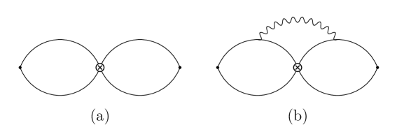
Figure 1: The leading-order perturbative contribution to the three-point correlator (a), and a non-factorizable perturbative contribution at next-to-leading-order (b).

In this section we describe the calculation of the spectral density functions using the OPE. The leading-order results are given by the bare quark loops shown in Figure 1(a). The cross denotes the insertion of any one of the four-quark operators $Q,Q_{S},R_{2},R_{3}$, and the solid dots can be either axial-vector or pseudoscalar interpolating currents. The analysis works very much the same for each of these eight possible cases. Corrections to the leading-order result come from two sources: higher-order perturbative corrections and non-perturbative corrections in the form of vacuum condensates. Our focus in this paper is on the vacuum condensate contributions, which we consider up to dimension six by calculating the gluon condensate, the mixed quark-gluon condensate, and the four-quark condensate.

The leading non-perturbative contributions involve the gluon condensate, a dimension-four object defined through the vacuum matrix element

$$\langle G_{\mu\nu}^{a}G_{\alpha\beta}^{b}\rangle=\frac{\delta^{ab}}{12(N_{c}^{2}-1)}(g_{\mu\alpha}g_{\nu\beta}-g_{\mu\beta}g_{\nu\alpha})\langle GG\rangle.$$ (29)

The non-factorizable corrections proportional to the gluon condensate are obtained by calculating the diagram shown in Figure 2(a) along with the three other permutations where the gluons are attached to different loops. Diagrams where the two gluons are attached to the same loop are factorizable and hence do not contribute to $\Delta B$.

The calculation is most easily performed using the external-field method [15]. The advantage of this technique is that the external gluon field can be expressed in terms of the field-strength tensor according to the relation

$$A^{a}_{\mu}(x)=\frac{1}{2}x^{\alpha}G^{a}_{\alpha\mu}+O(x^{2}).$$ (30)

This property allows for a direct extraction of the gluon condensate contributions from the diagrams in Fig 2(a), and also simplifies the calculation for the subleading operators $R_{2}$ and $R_{3}$. Since the operators $R_{2}$ and $R_{3}$ are evaluated at the point $x=0$, the diagrams where a gluon is emitted from the operator itself (the cross in the diagrams) vanish, and one need only consider derivative couplings, whose evaluation is essentially the same as for the leading-order operators $Q$ and $Q_{S}$.

We next consider the dimension-five contributions. These are proportional to the mixed quark-gluon condensate, which is defined through the matrix element

$$\langle\bar{s}_{\alpha}ig_{s}G_{\beta\eta}^{a}t^{a}s_{\rho}\rangle=\frac{\left(i\sigma_{\beta\eta}\right)_{\rho\alpha}}{48}\langle\bar{s}Gs\rangle.$$ (31)

The relevant non-factorizable diagrams are shown in Figure 2(b). As with the gluon condensate, the relation (30) leads to simplifications for the subleading operators $R_{2},R_{3}$. Also in this case one need not consider gluons emitted from the covariant derivative; moreover, the external strange-quark fields carry vanishing momentum, so derivatives can only act on the strange-quark field contracted inside the loop.

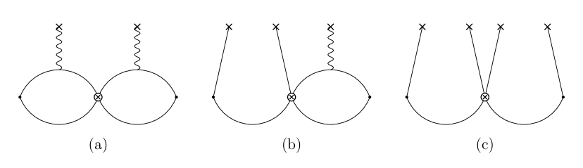
Figure 2: Non-factorizable contributions involving (a) the $\langle GG\rangle$ condensate, (b) the $\langle\bar{s}Gs\rangle$ condensate, and (c) the $\langle\bar{s}s\bar{s}s\rangle$ condensate.

Finally, we consider the dimension-six contributions involving the four-quark condensate. The relevant non-factorizable diagrams are shown in Figure 2(c). These vanish for the subleading operators $R_{2}$ and $R_{3}$, as can be seen by using (30) and then noting that the derivative terms act on the vacuum fields and thus vanish. For the leading-order operators $Q$ and $Q_{S}$ the contributions involve matrix elements of the form $\langle\bar{s}\Gamma_{1}s\bar{s}\Gamma_{2}s\rangle$ where the $\Gamma_{i}$ involve both Dirac and color indices. To evaluate these non-factorizable four-quark matrix elements we use the vacuum saturation approximation, by which the full matrix element is expressed as

$$\langle\bar{s}\Gamma_{1}s\bar{s}\Gamma_{2}s\rangle=\frac{1}{(4N_{c})^{2}}\left({\rm tr}\Gamma_{1}\,{\rm tr}\Gamma_{2}-{\rm tr}\Gamma_{1}\Gamma_{2}\right)\langle{\bar{s}}s\rangle^{2}.$$ (32)

This approximation dates back to the first applications of the sum rule method [16], and since then has been checked through numerical analysis in many physical channels. One particular study for vector-vector and axial-axial channels established that the factorization is accurate within 15-20% [17]. Upon using this approximation for the current correlator, we find that non-factorizable contributions from the four-quark condensate to sum rule for $Q$ and $Q_{S}$ also vanish. Details are given in the appendix.

We shall limit our OPE analysis to these non-perturbative condensates. To this level of accuracy, the OPE result for the spectral density can be written as

$$\Delta\rho_{i}(s_{1},s_{2})=\Delta\rho_{i}^{\rm GG}(s_{1},s_{2})\langle GG\rangle+\Delta\rho_{i}^{\rm sGs}(s_{1},s_{2})\langle\bar{s}Gs\rangle+\dots$$ (33)

for each of the eight cases. Explicit results for the $\Delta\rho_{i}$ can be found in the appendix. The result for the operator Q with an AV (PS) interpolating current was first obtained in [12] ([13]), while the others are new. The ellipsis refers to the corrections not taken into account in our analysis. These include contributions from the dimension six condensate $\langle f^{abc}G^{a}_{\mu\nu}G^{b}_{\nu\tau}G^{c}_{\tau\mu}\rangle$, whose numerical value is considered to be small [16]. An attempt to take into account condensates of operators of dimension 7 and even 8 was made in ref. [13] for the operator $Q$. We note, however, that the numerical values of these condensates are very uncertain and their effects small, and thus exclude them from the analysis.

More important are higher-order perturbative corrections. The next-to-leading order corrections are parametrically on the order of $\alpha_{s}(m_{b})/\pi\sim 0.06$ for $\alpha_{s}(m_{b})=0.2$. Non-factorizable perturbative corrections require the evaluation of three-loop diagrams such as that shown in Figure 1(b). These were calculated in [18] for the leading-order operator $Q$, but are unknown for the other cases.

As an example and to introduce notation we give here the explicit expression for the $Q_{S}$ operator with a pseudoscalar interpolating current:

$$\Delta\rho_{\rm PS}(s_{1},s_{2}) = \frac{1}{48\pi^{2}}\langle\frac{\alpha_{s}}{\pi}GG\rangle\frac{1}{s_{1}s_{2}}\left(\frac{s_{1}s_{2}}{2}(6-3z_{1}-3z_{2}+z_{1}z_{2})+(p_{1}p_{2})^{2}z_{1}z_{2}\right)$$ (34)

$$+\frac{1}{16\pi^{2}}\langle\bar{s}Gs\rangle m_{b}\left((-2+z_{1})\delta(s_{2}-m_{b}^{2})+(-2+z_{2})\delta(s_{1}-m_{b}^{2})\right)$$

Here $z_{i}=m_{b}^{2}/s_{i}$, and $\delta(s_{i}-m_{b}^{2})$ is the Dirac $\delta$ function. At the physical point $q^{2}=(p_{1}-p_{2})^{2}=0$ the scalar product $(p_{1}p_{2})$ should be understood as $(p_{1}p_{2})=(s_{1}+s_{2})/2$.

We also need the HQET expansion of the spectral density, which we obtain by using $s_{i}=(m_{b}+E_{i})^{2}$ and expanding to lowest order in $E_{i}/m_{b}$. In this case this limit reads

$$\Delta\rho_{\rm PS}^{\rm HQET}(E_{1},E_{2})=\frac{1}{48\pi^{2}}\frac{1}{4\pi^{2}}\bigg{[}\frac{3}{2}\langle g_{s}^{2}GG\rangle-6\pi^{2}\langle\bar{s}Gs\rangle\left(\delta(E_{1})+\delta(E_{2})\right)\bigg{]}.$$ (35)

4 The bag parameters from finite energy sum rules

In this section we present the sum-rule results for the $\Delta B_{i}$ using the finite energy sum rules (20, 21) evaluated at leading order in the HQET approximation. We first give simple analytical expressions for the $\Delta B_{i}$, obtained by relating the sum-rule parameter $s_{0}$ to the $B$-meson decay constant $f_{B}$, thereby eliminating one parameter. Upon inserting numerical values it becomes clear that $\Delta B$ is suppressed by a small scale ratio, independent of the particular operator being considered.

4.1 The choice of duality interval

The sum-rule results for the $\Delta B_{i}$ depend on the choice of the parameter $s_{0}$ defining the upper limit in the duality integrals in (20), (27). For the hadronic part the best accuracy is obtained by considering small values of $s_{0}$ for which saturation by the ground state is a justified approximation. The OPE side, on the other hand, is best suited for inclusive quantities for which perturbation theory is valid. The quantity $s_{0}$ must be chosen in such a way as to balance between these two cases, and the exact value to use is thus a matter of judgement. A useful guide for determining its value is to use QCD sum rules for the matrix elements (14) to express $s_{0}$ in terms of the decay constant $f_{B}$. This makes the finite energy sum rule analysis of the three-point correlator parametrically free and the analytical results simple, allowing us to discuss qualitative features which are less transparent in a purely numerical analysis.

The two-point sum rule for the decay constant $f_{B}$ is obtained in the standard way. One evaluates the spectral density for the two-point function in both a phenomenological hadronic picture and in the OPE. Equating the integrals of the two spectral densities over a duality interval gives a result for the decay constant $f_{B}$. We calculate the OPE spectral density by evaluating the two-point function in its crudest approximation, including only the bare quark loop. For the two-point function of axial vector currents we have

$$\rho^{{\rm OPE}}_{\rm AV}(s)=\frac{1}{4\pi^{2}}(1-z)^{2}(1+2z),\qquad z=m_{b}^{2}/s.$$ (36)

For the phenomenological spectral density we have

$$\rho^{{\rm PH}}_{\rm AV}(s)=f_{B}^{2}\delta(s-M_{B}^{2}).$$ (37)

Equating the two expressions as in (19) (local duality finite energy sum rules [19]) yields

$$(2\pi f_{B})^{2}=s_{0}(1-z_{0})^{3}\qquad({\rm AV\,current})$$ (38)

$z_{0}=m_{b}^{2}/s_{0}$. We see that the duality interval parameter $s_{0}$ can be expressed through $f_{B}$ and $m_{b}$. We rewrite the expression (38) in a form suitable for HQET by substituting $s_{0}=(m_{b}+E_{0})^{2}$ and expanding in the ratio $E_{0}/m_{b}\ll 1$. Retaining the leading term of the expansion we find an equation relating the HQET sum-rule parameter $E_{0}$ with the physical quantity $f_{B}$:

$$(2\pi f_{B})^{2}\approx\frac{8}{m_{b}}E_{0}^{3}\qquad{\rm(AV\,current)}.$$ (39)

For $f_{B}=240~{}{\rm MeV}$ and $m_{b}=4.8~{}{\rm GeV}$ one finds $E_{0}=1.1~{}{\rm GeV}$. Repeating the analysis for the pseudoscalar interpolating current, where (neglecting the strange-quark mass)

$$\rho^{\rm OPE}_{\rm PS}=\frac{3}{8\pi^{2}}s\left(1-\frac{m_{b}^{2}}{s}\right)^{2}$$ (40)

we have in the HQET limit

$$(2\pi f_{B})^{2}\approx\frac{4}{m_{b}}E_{0}^{3}\qquad{(\rm PS\,current)}$$ (41)

which gives $E_{0}=1.4~{}{\rm GeV}$. Thus, the numerical value of the duality interval fluctuates depending on the channel chosen for its determination. At any rate the results are consistent with the general expectation that the scale of duality in hadronic physics is about $1~{}{\rm GeV}$.

This idea of determining the value of the duality interval from two-point sum rules works well quantitatively also for light quarks. Indeed, by comparison, for light $u$-, $d$-quarks one finds the relation $(2\pi f_{\pi})^{2}=s_{0}$, which gives $s_{0}=0.7~{}{\rm GeV}^{2}$ for $f_{\pi}=130~{}{\rm MeV}$. This is the actual duality parameter for sum rules in the axial-vector channel of light mesons [20].

The relations (39) and (41) allow for a simple parameter-free analysis in the HQET limit. They show the correct scaling for the semileptonic decay constant with the heavy quark mass, $f_{B}\sim 1/\sqrt{m_{b}}$, and upon using them in the sum rules the explicit results for the bag parameters become independent of $m_{b}$, as appropriate for hadronic quantities. For a quantitative comparison with full QCD higher-order corrections in $E_{0}/m_{b}$ are important numerically, as the expansion parameter $E_{0}/m_{b}\approx 0.2$ is not very small. We see this further in our analysis with Borel sum rules.

4.2 Finite energy sum rules in HQET

In this section we present the analysis using the finite energy sum rules (20, 21) expanded to leading order in HQET. We work at leading order in $\alpha_{s}$ and ignore even leading-log resummation. At this level of precision the HQET approximation can be obtained by first evaluating matrix elements in full QCD and then expanding as described in Section 2.1. To evaluate the phenomenological side of the sum rules we use the explicit expressions (7), and to evaluate the OPE side we use the HQET results from the appendix.

4.2.1 Leading order operators $Q$ and $Q_{S}$

We start our analysis with the leading-order operators $Q$ and $Q_{S}$, for which we describe the procedure in some detail.

Operator $Q$ with axial vector interpolating current:

On the phenomenological side of the sum rule (20) we have after subtracting the factorized contribution (cf. eq. 27)

$$I^{PH}=\frac{8}{3}\Delta Bf_{B}^{4}M_{B}^{2}\approx\frac{8}{3}\Delta Bf_{B}^{4}m_{b}^{2},$$ (42)

where in the second equality we used the HQET limit. To evaluate the OPE side in the same limit we use $s_{i}=(m_{b}+E_{i})^{2}$ in the QCD spectral density from the Appendix and expand to leading order in $E_{i}/m_{b}$, leaving

$$\Delta\rho^{OPE}(s_{1},s_{2}) = \frac{1}{48\pi^{2}}\langle\frac{\alpha_{s}}{\pi}GG\rangle\frac{(p_{1},p_{2})}{s_{1}s_{2}}2z_{1}z_{2}(-3+z_{1}+z_{2}-2z_{1}z_{2})$$ (43)

$$\approx \frac{1}{48\pi^{2}}\frac{\langle g_{s}^{2}G^{2}\rangle}{4\pi^{2}}\frac{1}{m_{b}^{2}}(-6).$$

Performing the integration on the OPE side we arrive at the sum rule

$$\frac{8}{3}\Delta B(2\pi f_{B})^{4}=-2\langle g_{s}^{2}G^{2}\rangle\frac{E_{0}^{2}}{m_{b}^{2}}.$$ (44)

Using (39) to trade $(2\pi f_{B})^{4}$ for $E_{0}$ we find the simple result

$$\Delta B=-\frac{3}{256}\frac{\langle g_{s}^{2}G^{2}\rangle}{E_{0}^{4}}.$$ (45)

The result for the non-perturbative bag parameter is independent of $m_{b}$, as it should be in the HQET limit, where dynamical quantities depend on soft physics only. This fact can be noticed already from (44) by using the scaling relation $f_{B}\sim 1/\sqrt{m_{b}}$ deduced from (39). Taking the value of the gluon condensate as $\langle g_{s}^{2}G^{2}\rangle=0.48~{}{\rm GeV}^{4}=(0.83~{}{\rm GeV})^{4}$ [16] we have

$$\Delta B=-0.006,$$ (46)

at $E_{0}=1~{}{\rm GeV}$, which shows that the non-factorizable contribution to the matrix element is tiny.

Examining the expressions for $\Delta B$, one sees that it is the suppression by the combination of variables $(2\pi f_{B})^{4}m_{b}^{2}/E_{0}^{2}=64E_{0}^{4}=(3.3~{}{\rm GeV})^{4}$ which leads to this result. This combination does not scale with $m_{b}$ in the HQET limit and $f_{B}$ is further enhanced by $N_{c}^{1/2}$ in the large-$N_{c}$ limit. Since the scale of the gluon condensate is given by $(0.83~{}{\rm GeV})^{4}$, the result for $\Delta B$ is proportional to the fourth power of a small number. In the absence of any accidental numerical enhancement of the coefficients, which we do not see, the “natural” size of the deviations from factorization is extremely small.

The answer (46) is the leading-order HQET result. To get a feel for the size of the subleading terms, we list the next few terms in the expansion of the OPE spectral density:

$$\Delta B = -\frac{3}{256}\frac{\langle g_{s}^{2}G^{2}\rangle}{E_{0}^{4}}\left[1-\frac{11}{3}\frac{E_{0}}{m_{b}}+10\left(\frac{E_{0}}{m_{b}}\right)^{2}-\frac{215}{9}\left(\frac{E_{0}}{m_{b}}\right)^{3}+\dots\right]$$ (47)

$$= -\frac{3}{256}\frac{\langle g_{s}^{2}G^{2}\rangle}{E_{0}^{4}}\left[1-0.8+0.4-0.2+\dots\right]$$

$$= -\frac{3}{256}\frac{\langle g_{s}^{2}G^{2}\rangle}{E_{0}^{4}}\left(0.5\right),$$

where we used $m_{b}=4.8~{}{\rm GeV}$ and to obtain the last line we evaluated the full QCD result. This shows that the subleading terms are not small, and that keeping only the leading-order term misses the full QCD result by a factor of two, at least at $E_{0}=1~{}{\rm GeV}$. Given the small size of $\Delta B$ the factor of two is numerically irrelevant, and is actually within the uncertainties of the analysis. We return to this point in Section 6, using the subleading operator $R_{2}$ as an additional example.

Operator $Q$ with pseudoscalar interpolating current:

We can repeat the computation using a pseudoscalar interpolating current. At leading order in $1/m_{b}$ we neglect $m_{s}$ and expand as before, finding

$$\frac{8}{3}\Delta B(2\pi f_{B})^{4}=\frac{1}{m_{b}^{2}}\left(-\langle g_{s}^{2}G^{2}\rangle E_{0}^{2}+8\pi^{2}\langle\bar{s}Gs\rangle E_{0}\right).$$ (48)

The mixed quark-gluon condensate is parameterized as $\langle\bar{s}Gs\rangle=m_{0}^{2}\langle\bar{s}s\rangle$. For numerical evaluation we use $m_{0}^{2}=0.8~{}{\rm GeV}^{2}$ [21, 22] and $\langle\bar{s}s\rangle=0.8\langle\bar{u}u\rangle$ [23, 24]. For the light quark condensate $\langle\bar{u}u\rangle$ we take $\langle\bar{u}u\rangle=(-0.24~{}{\rm GeV})^{3}$. A convenient normalization for the mixed quark-gluon condensate is

$$\pi^{2}\langle\bar{s}Gs\rangle=-0.1~{}{\rm GeV}^{5}=(-0.63~{}{\rm GeV})^{5},$$ (49)

which is of the same order of magnitude as $\langle g_{s}^{2}G^{2}\rangle$ and is really given by the hadronic scale of $1~{}{\rm GeV}$ (or say by the $\rho$-meson mass $m_{\rho}=770~{}{\rm MeV}$). We see that all dimensionful quantities are on the order of the fundamental QCD scale of $1~{}{\rm GeV}$ as expected.

Using (39) to eliminate $f_{B}$ one finds

$$\Delta B=-\frac{3}{256}\left(\frac{\langle g_{s}^{2}G^{2}\rangle}{2E_{0}^{4}}-\frac{4\pi^{2}\langle\bar{s}Gs\rangle}{E_{0}^{5}}\right)=-\frac{3}{256}\left(0.24+0.4\right)=-0.008$$ (50)

at $E_{0}=1~{}{\rm GeV}$. The result is more or less the same as with the axial-vector interpolating current but the structure of contributions changed. The gluon condensate contributes less and mixed quark-gluon gives a contribution (it was zero for the axial-vector case).

Using $E_{0}^{PS}=1.4~{}{\rm GeV}$ from (41) for the pseudoscalar channel one finds

$$\Delta B=-\frac{3}{64}\left(\frac{\langle g_{s}^{2}G^{2}\rangle}{2(E_{0}^{PS})^{4}}-\frac{4\pi^{2}\langle\bar{s}Gs\rangle}{(E_{0}^{PS})^{5}}\right)=-\frac{3}{64}\left(0.062+0.074\right)=-0.006$$ (51)

which coincides with the previous result from the AV current. Even though it is more proper to use the result (41) for the PS channel, for the remaining operators we shall use (39) in both the AV and PS channel; the differences are very small.

Operator $Q_{S}$ with axial vector interpolating current:

Repeating the analysis for $Q_{S}$ with an axial-vector current we find the sum rule

$$-\frac{5}{3}\Delta B_{S}(2\pi f_{B})^{4}=\frac{1}{m_{b}^{2}}\left(\frac{1}{6}\langle g_{s}^{2}G^{2}\rangle E_{0}^{2}-4\pi^{2}\langle\bar{s}Gs\rangle E_{0}\right)$$ (52)

and

$$\Delta B_{S}=-\frac{1}{640}\left(\frac{\langle g_{s}^{2}G^{2}\rangle}{E_{0}^{4}}-24\pi^{2}\frac{\langle\bar{s}Gs\rangle}{E_{0}^{5}}\right)=-\frac{1}{640}\left(0.48+2.4\right)=-0.005$$ (53)

again a very small number. Note that the result is dominated by the contribution of the mixed quark-gluon condensate, even though it is formally subleading compared to the gluon condensate. This is a general situation, as contributions from the gluon condensate are often small numerically.

Operator $Q_{S}$ with pseudoscalar interpolating current:

Repeating for the pseudoscalar current we have

$$\Delta B_{S}=-\frac{3}{640}\left(\frac{\langle g_{s}^{2}G^{2}\rangle}{E_{0}^{4}}-8\pi^{2}\frac{\langle\bar{s}Gs\rangle}{E_{0}^{5}}\right)=-\frac{3}{640}\left(0.48+0.8\right)=-0.006.$$ (54)

The coefficients of the gluon and mixed quark-gluon condensates changed, but their sum is very close to that obtained with the axial-vector current.

We conclude that the deviation from factorization is tiny just because of the scales involved. No surprisingly big numbers or drastic cancellations occurred in the analysis.

4.2.2 Subleading operators $R_{2}$ and $R_{3}$

The analysis is essentially unchanged for the subleading operators $R_{2}$ and $R_{3}$. The new feature is the appearance of the parameter $\bar{\Lambda}=M_{B}-m_{b}$ even at leading-order in the HQET expansion (numerically $M_{B}=5367.5\pm 1.8~{}{\rm MeV}$ [25]). It enters through the expansion of the matrix elements (7), which read

$$\langle\bar{B}|R_{2}|B\rangle_{\rm HQET} = -f_{B}^{2}m_{b}^{2}\left(2\bar{\Lambda}m_{b}\right)\left(1-\frac{1}{N_{c}}\right)B_{2}$$ (55)

$$\langle\bar{B}|R_{3}|B\rangle_{\rm HQET} = f_{B}^{2}m_{b}^{2}\left(2\bar{\Lambda}m_{b}\right)\left(1+\frac{1}{2N_{c}}\right)B_{3}.$$ (56)

This $\bar{\Lambda}/m_{b}$ power suppression of the matrix elements on the phenomenological side of the sum rules is compensated by an $E_{0}/m_{b}$ suppression from the OPE spectral densities. Then, up to a factor of $E_{0}/2\bar{\Lambda}\sim 1$, the magnitude of $\Delta B$ for the subleading operators is fixed by the same scale ratios as before, and as with the leading-order case there are no large deviations from factorization.

Operator $R_{2}$ with axial vector interpolating current:

$$-2\bar{\Lambda}m_{b}(2\pi f_{B})^{4}\frac{2}{3}\Delta B_{2}=\frac{1}{m_{b}^{2}}\left(\langle g_{s}^{2}G^{2}\rangle m_{b}E_{0}^{3}\left(-\frac{3}{2}\right)-2\pi^{2}\langle\bar{s}Gs\rangle m_{b}E_{0}^{2}\right)$$ (57)

Notice that for this subleading operator the phenomenological and OPE sides of the sum rule are suppressed by the hadronic scales $\bar{\Lambda}$ and $E_{0}$ respectively. This is explicit in the HQET expressions but not in the QCD ones. Using (39) and taking $\bar{\Lambda}=0.5~{}{\rm GeV}$

$$\Delta B_{2}=\frac{E_{0}}{2\bar{\Lambda}}\frac{9}{256}\left(\frac{\langle g_{s}^{2}G^{2}\rangle}{E_{0}^{4}}+\frac{4\pi^{2}\langle\bar{s}Gs\rangle}{3E_{0}^{5}}\right)=\frac{9}{256}\left(0.48-0.13\right)=0.012.$$ (58)

We see that $\Delta B_{2}$ is again very small, although this time it is a positive number instead of a negative one.

Operator $R_{2}$ with pseudoscalar interpolating current:

$$\Delta B_{2}=\frac{E_{0}}{2\bar{\Lambda}}\frac{3}{256}\left(\frac{\langle g_{s}^{2}G^{2}\rangle}{E_{0}^{4}}-\frac{4\pi^{2}\langle\bar{s}Gs\rangle}{E_{0}^{5}}\right)=\frac{3}{256}\left(0.48+0.4\right)=0.010.$$ (59)

Operator $R_{3}$ with the axial vector interpolating current:

$$\frac{7}{6}\Delta B_{3}=\frac{E_{0}}{2\bar{\Lambda}}\frac{1}{64}\left(\frac{\langle g_{s}^{2}G^{2}\rangle}{E_{0}^{4}}\left(\frac{1}{6}\right)-\frac{2\pi^{2}\langle\bar{s}Gs\rangle}{E_{0}^{5}}\right)=\frac{1}{64}\left(0.08+0.2\right)=0.004.$$ (60)

and

$$\Delta B_{3}=0.004$$ (61)

Operator $R_{3}$ with pseudoscalar interpolating current:

$$\frac{7}{6}\Delta B_{3}=\frac{E_{0}}{2\bar{\Lambda}}\frac{1}{64}\left(\frac{\langle g_{s}^{2}G^{2}\rangle}{E_{0}^{4}}\left(\frac{1}{4}\right)-\frac{\pi^{2}\langle\bar{s}Gs\rangle}{E_{0}^{5}}\right)=\frac{1}{64}\left(0.12+0.1\right)=0.003$$ (62)

and

$$\Delta B_{3}=0.003.$$ (63)

We can summarize by saying that the finite energy sum rules within the HQET approximation suggest that factorization is perfectly precise, if only non-perturbative condensate effects are taken into account. The bag parameter $B_{2}$ has the largest violation of factorization, but it is still very small in absolute terms, approximately 1%.

5 The bag parameters from Borel sum rules

We have seen in the previous section that the deviations from factorization for both the leading and subleading operators are very small. In this section we perform a more thorough numerical analysis using Borel sum rules. This serves to confirm these results and to show that it is possible to impose very conservative error estimates without altering this conclusion. We also use the numerics to compare the HQET and full QCD results.

5.1 Borel sum rules in full QCD

Figure 3: Plot of $-\Delta B$ vs. $M^{2}\,({\rm GeV}^{2})$ for the leading-order operators $Q$ and $Q_{S}$ and $\Delta B$ for the subleading operators $R_{2}$ and $R_{3}$ with the Borel sum rules in full QCD. The short-dashed lines are obtained using an axial vector interpolating current, and the long-dashed lines using a pseudoscalar current. The parameter values are given by $m_{b}=4.2$ GeV, $f_{B_{s}}=240$ MeV, $s_{0}=36~{}{\rm GeV}^{2}$, and $m_{s}$ as explained in the text.

The Borel sum rules in full QCD are evaluated according to (22) and the analogous expression for the pseudoscalar interpolating current. Although it is possible to evaluate the Borel integrals analytically, the results are quite lengthy and we do not need them for this purely numerical analysis.

To evaluate the sum rules, we must first give numerical values for the QCD parameters $f_{B_{s}}$, $m_{b}$, and $m_{s}$. For the decay constant we choose $f_{B_{s}}=240~{}{\rm MeV}$ as the default value. For the $b$-quark mass one can take the pole mass or the $\overline{\rm MS}$ mass. The pole mass is $m_{b}^{pole}=4.8~{}{\rm GeV}$ while the $\overline{\rm MS}$ value is $m_{b}^{\overline{\rm MS}}=4.2~{}{\rm GeV}$ [26, 27]. For the full QCD analysis the $\overline{\rm MS}$ mass is more appropriate. However, since we are working to lowest order in $\alpha_{s}$, we cannot distinguish these two quark-mass definitions, and the difference can be accounted for as an additional uncertainty in $\Delta B$. This difference would be under control if $\alpha_{s}$ corrections were taken into account.

The strange-quark mass appears on the OPE side of the sum rules for all channels, and in the phenomenological side for the case of the pseudoscalar interpolating current. We have seen that $\Delta B$ is extremely small in all cases, and the effects of a non-zero strange quark mass do little to alter this. We choose to keep it non-zero on the phenomenological side for the leading-order operators $Q$ and $Q_{S}$, using $m_{s}=100~{}{\rm MeV}$. Keeping it non-zero in the OPE spectral densities complicates the analytical expressions without changing the final results in a significant way. For the subleading operators it is consistent to set it to zero at this order in the heavy-quark expansion.

The results for $\Delta B$ vs. the Borel parameter $M^{2}$ for each operator are shown in Figure 3. The two lines in each plot are obtained by using an axial-vector and pseudoscalar interpolating current. All results have a reasonable stability region in $M^{2}$ at $10~{}{\rm GeV}^{2}<M^{2}<20~{}{\rm GeV}^{2}$. There is some dependence on the choice of interpolating current, which as we will see later is within the uncertainties of the analysis. We note again that $\Delta B$ is positive for the subleading operators $R_{2}$ and $R_{3}$, whereas it is negative for the leading operators $Q$ and $Q_{S}$.

5.2 Borel sum rules in HQET

Figure 4: Plots of $(-)\Delta B$ vs. $W~{}({\rm GeV})$ obtained with the Borel sum rules in HQET. The short-dashed lines are obtained using an axial vector interpolating current, and the long-dashed lines using a pseudoscalar current. We take $\bar{\Lambda}=600$ MeV, $m_{b}=4.8~{}{\rm GeV}$, $f_{B_{s}}=240$ MeV, and $2E_{0}=2.5~{}{\rm GeV}$.

The Borel sum rules in HQET are performed according to (28) and analogously for the PS interpolating current. We focus on numerical results, although the analytical results for the Borel integrals are very simple. In fact, they reduce to those from the finite energy sum rules in the limit $W\to\infty$. In contrast to our treatment of the finite energy sum rules, however, in our numerical studies we treat $E_{0}$ and $f_{B}^{2}m_{b}$ as free parameters. We again use $f_{B_{s}}=240~{}{\rm MeV}$ as the default value. While in the QCD calculation the $\overline{\rm MS}$ mass was more natural, in HQET the pole mass appears in the construction of the effective theory and is more natural. We use $m_{b}^{pole}=4.8~{}{\rm GeV}$.

The results for $\Delta B$ vs. the HQET Borel parameter $W$ for each operator are shown in Figure 4. The plots are stable in the region $1~{}{\rm GeV}<W<2.5~{}{\rm GeV}$, which is rather typical for Borel sum rules in HQET. The values of $\Delta B$ in the stability range are close to those in the QCD plots in Figure 3. The one noticeable exception is $R_{2}$, where the HQET values are about twice as large as the QCD ones. We comment further on this in the next section.

Operator	$\Delta B(\%)$ QCD	$\Delta B(\%)$ HQET
$Q$	$-0.6\pm 0.5$	$-0.6\pm 0.5$
$Q_{S}$	$-0.5\pm 0.4$	$-0.6\pm 0.4$
$R_{2}$	$0.3\pm 0.3$	$0.8\pm 0.7$
$R_{3}$	$0.3\pm 0.2$	$0.3\pm 0.2$

Table 1: A summary of the results.

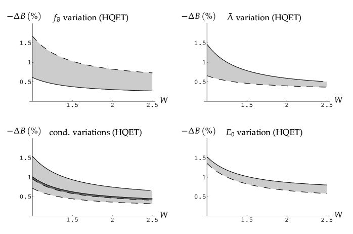
Figure 5: Plots showing $-\Delta B$ vs. $W~{}({\rm GeV})$ for the case of the $Q_{S}$ operator, axial-vector current, using a range of parameter values in the HQET sum rule. The plots are made by varying the parameters as explained in the text. For the condensate variations, the dark-gray band corresponds to the gluon condensate and the larger light-gray band to the quark-gluon condensate variation. In each case, the dashed line corresponds to the lower border of the parameter range (e.g. $f_{B_{s}}=210$ MeV) and the solid line to the upper border (e.g. $f_{B_{s}}=270$ MeV).

6 Final results and discussion

We now present our final numerical results and estimate the associated uncertainties. The results are summarized in Table 1.

To obtain the table entries for full QCD, we fix the Borel parameter at $M^{2}=15~{}{\rm GeV}^{2}$ and vary the other parameters in the ranges

$${\underline{\rm QCD}}$$

$$210~{}{\rm MeV}<f_{B_{s}}<270~{}{\rm MeV}$$

$$4~{}{\rm GeV}<m_{b}<4.4~{}{\rm GeV}$$

$$32~{}{\rm GeV}^{2}<s_{0}<40~{}{\rm GeV}^{2}$$

where the default values lie in the center of the above ranges. We also vary the condensates about their default values by $\pm 30\%$. For a given case, we find upper and lower values of $\Delta B$ to identify the error ranges. For the $f_{B_{s}},m_{b}$ and $s_{0}$ variations the ranges are asymmetric; in those cases we use the larger deviation in the error analysis. Finally, we add the uncertainties from each of the five variations in quadrature, and average the results from the axial-vector and pseudoscalar interpolating currents to obtain the results quoted in the table.

The procedure is the same for the HQET sum rules, although the set of parameters is different. This time we fix the Borel parameter at $W=2~{}{\rm GeV}$ and the $b$-quark mass at $m_{b}=4.8~{}{\rm GeV}$, and vary the other parameters in the ranges

$${\underline{\rm HQET}}$$

$$210~{}{\rm MeV}<f_{B_{s}}<270~{}{\rm MeV}$$

$$500~{}{\rm MeV}<\bar{\Lambda}<700~{}{\rm MeV}$$

$$1~{}{\rm GeV}<E_{0}<1.5~{}{\rm GeV}$$

where the default values lie in the center of the above ranges. The condensates are again varied by $\pm 30\%$ about their default values. The final table entries are obtained as for the QCD case.

To illustrate the uncertainty associated with each parameter variation, we choose as an example the $Q_{S}$ operator with an axial-vector interpolating current in HQET. The range of $\Delta B$ associated with each variation is represented by the gray bands in Figure 5. It is seen that the largest errors are associated with the value of the decay constant $f_{B}$. This is not surprising, since the explicit results scale as $1/f_{B}^{4}$. At the default value $W=2$ the dependence on $\bar{\Lambda}$ and $E_{0}$ is moderate. The results depend linearly on the condensates and at $W=2$ the uncertainty due to the condensates is comparable with that due to $f_{B}$.

In all cases except for $R_{2}$, our central values for $\Delta B$ in QCD and HQET turned out to be (nearly) equal. However, in interpreting this result, one should be clear that not only the bag parameters, but also the QCD parameters $f_{B}$ and $M_{B}$ have an expansion in $1/m_{b}$. When comparing the QCD result with the HQET result, we have no means of disentangling the corrections to $f_{B}$ and $M_{B}$ from those to $B_{i}$, so it is not obvious whether numerical discrepancies are due to corrections to the bag parameters, form factors, meson masses, the OPE, or even our choices of sum rule parameters. The conclusion to make is that the leading-order expansion and the full results are consistent with one another in all cases, within the uncertainties of the analysis.

This said, further investigation of the HQET series for the OPE spectral densities for $R_{2}$ reveals some interesting features. As an example, we take the piece of the spectral density for $R_{2}$ multiplying $\langle GG\rangle$ as calculated with an axial-vector current, and consider some higher-order terms in the $E_{0}/m_{b}$ expansion of the integrated spectral density. Using the notation $x_{i}=E_{i}/m_{b}$, integrating over the square $0<x_{i}<x_{0}$, and normalizing to the leading-order term in the $x_{0}=E_{0}/m_{b}$ expansion, we have

$$\frac{4\int dx_{1}dx_{2}\rho^{\rm GG}(x_{1},x_{2})}{4\int dx_{1}dx_{2}(-9/2x_{1}-9/2x_{2})}=1-\frac{154}{27}x_{0}+\frac{560}{27}x_{0}^{2}+\dots=1.0-1.2+0.9+\dots$$ (64)

To derive the numbers we used $x_{0}=E_{0}/m_{b}\approx 0.2$ for $E_{0}=1~{}{\rm GeV}$. The second and third terms are as large as the first, and the corrections do not fall below 10% until the sixth term, so the “HQET” expansion is not well behaved. We put HQET in quotes, because the expansion is just the diagrammatic one, not a rigorous one in terms of operators. It would be interesting to see whether this poor convergence persists even with a more careful treatment of the subleading corrections. If so, this would have important implications for lattice QCD results, where corrections to the HQET limit are not easy to control.

In quoting our final results, we used only those obtained from the Borel sum rules. However, one can work with either finite energy or Borel sum rules. Finite energy sum rules can be obtained from Borel sum rules in the limit $M^{2}\to\infty$ and are therefore more sensitive to the model of the continuum. We used both and saw little difference. Our sum rule analysis is by no means unique. For instance, one can change the duality integrals by modifying each side of the sum rule in the same way (for instance by dividing both sides by $(s_{1}s_{2})$). This definitely changes the shape of the curves and can provide better stability. However, our main point is that $\Delta B$ is so small that we need not be too sophisticated with the sum rules analysis. The splitting into factorized and non-factorized parts is powerful and useful precisely because the absolute value of $\Delta B$ turns out to be small. Even with very conservative error estimates the results are numerically informative, and our final results – the range for the values of $\Delta B$ – rather reliable.

It is instructive to compare our approach to lattice QCD. In the lattice approach the parameter $B$ is computed as a whole, since a splitting into factorizable and non-factorizable parts is not possible at the level of simulation. Then for the computation of the parameter $B$ (and not $\Delta B$ directly) even good accuracy of the method (say, about 20%, a typical accuracy in hadronic physics) gives a less precise statement about factorization than our technique.

Our analysis was limited to leading order in perturbative corrections. A more accurate determination would require the computation of the next-to-leading order perturbative contributions. These involve three-loop diagrams and this is a non-trivial task. Results are nonetheless available for the operator $Q$ [18], where it was shown that these corrections amount to about 10%. For the other operators, we can say only that the corrections are parametrically on the order of $\alpha_{s}/\pi$ and are also expected to be around $10\%$. Thus, a qualitative prediction of the sum-rule analysis is that deviations from factorization are suppressed either by scale ratios or by the strong-coupling constant and are therefore small.

7 Conclusions

We used QCD sum rules to calculate the bag parameters for the leading and next-to-leading order operators in the $1/m_{b}$ expansion of the transition operator used to analyze $B_{s}-\bar{B}_{s}$ mixing. We found that the violation of the factorization approximation for the matrix elements of both the leading and subleading operators due to non-perturbative vacuum condensate contributions is well under control and small. Our final results for the parameters $\Delta B_{i}=B_{i}-1$ are

$$\Delta B|_{Q} = -0.6\pm 0.5\%$$

$$\Delta B|_{Q_{S}} = -0.5\pm 0.4\%$$

$$\Delta B|_{R_{2}} = 0.3\pm 0.3\%$$

$$\Delta B|_{R_{3}} = 0.3\pm 0.2\%$$

We believe that our very conservative error estimates make our final quantitative results (the range for the values of $\Delta B$) rather reliable.

Our result that the non-perturbative contributions to the $\Delta B_{i}$ are extremely small means that the non-factorizable contributions to the matrix elements are most likely dominated by calculable perturbative effects. We did not attempt to include the next-to-leading order perturbative contributions in our analysis. Our naive expectation, based on the existing calculations for the operator $Q$, is that these corrections can contribute an additional $\pm 10\%$. To clarify this point would require the evaluation of the set of three-loop diagrams appearing in the perturbative analysis.

Acknowledgements AAP thanks the Particle Theory Group of Siegen University where this work was done during his stay as a Mercator Guest Professor (Contract DFG SI 349/10-1). BDP acknowledges the support of the SFB/TR09 “Computational Particle Physics”. This work was supported by the German National Science Foundation (DFG) under contract MA 1187/10-1 and by the German Ministry of Research BMBF under contract 05HT6PSA.

8 Appendix

Here we compile the results for the condensate contributions to the OPE spectral density in each of the eight cases. For the axial-vector current we single out the scalar amplitude multiplying the structure tensor structure $p_{1}^{\mu}p_{2}^{\nu}$. For the pseudoscalar interpolating current there is only one amplitude as the correlation function is a scalar.

8.1 Spectral densities for $Q$

For the AV interpolating current we have

$$\Delta\rho_{\rm AV} = \frac{1}{48\pi^{2}}\langle\frac{\alpha_{s}}{\pi}GG\rangle\frac{1}{s_{1}s_{2}}(p_{1}p_{2})2z_{1}z_{2}(-3+z_{1}+z_{2}-2z_{1}z_{2})$$ (65)

$$\approx \frac{1}{48\pi^{2}}\frac{1}{4\pi^{2}}\frac{1}{m_{b}^{2}}\bigg{[}-6\langle g_{s}^{2}G^{2}\rangle\bigg{]}$$ (66)

where $z=m_{b}^{2}/s$ and we omit the factor $\theta(s_{i}-m_{b}^{2})$ setting the lower limits of integration for the $s_{i}$. The factor $(p_{1}p_{2})=s_{1}/2+s_{2}/2$ for $q^{2}=0$. To take the heavy-quark limit in the second line we used $s_{i}=m_{b}^{2}(1+x_{i})^{2}$ and expanded to lowest order in $x_{i}=E_{i}/m_{b}$.

For the PS interpolating current:

$$\Delta\rho_{\rm PS} = \frac{1}{48\pi^{2}}\langle\frac{\alpha_{s}}{\pi}GG\rangle\frac{1}{s_{1}s_{2}}(p_{1}p_{2})m_{b}^{2}3(-2+z_{1}+z_{2}-z_{1}z_{2})$$ (67)

$$+ (p_{1}p_{2})\frac{1}{16\pi^{2}}\langle\bar{s}Gs\rangle m_{b}\left(\frac{1}{s_{1}}2z_{1}\delta(s_{2}-m_{b}^{2})+\frac{1}{s_{2}}2z_{2}\delta(s_{1}-m_{b}^{2})\right)$$ (68)

$$\approx \frac{1}{48\pi^{2}}\frac{1}{4\pi^{2}}\bigg{[}-3\langle g_{s}^{2}G^{2}\rangle+12m_{b}\pi^{2}\langle\bar{s}Gs\rangle\left(2\delta(s_{2}-m_{b}^{2})+2\delta(s_{1}-m_{b}^{2})\right)\bigg{]}$$ (69)

8.2 Spectral densities for $Q_{S}$

AV interpolating current:

$$\Delta\rho_{\rm AV} = \frac{1}{48\pi^{2}}\langle\frac{\alpha_{s}}{\pi}GG\rangle\frac{m_{b}^{2}}{s_{1}s_{2}}\frac{1}{2}(6-3(z_{1}+z_{2})+z_{1}z_{2})$$ (70)

$$+ \frac{1}{16\pi^{2}}\langle\bar{s}Gs\rangle m_{b}\left(\frac{1}{s_{1}}(-2+z_{1})\delta(s_{2}-m_{b}^{2})+\frac{1}{s_{2}}(-2+z_{2})\delta(s_{1}-m_{b}^{2})\right)$$

$$\approx \frac{1}{48\pi^{2}}\frac{1}{4\pi^{2}}\frac{1}{m_{b}^{2}}\bigg{[}\frac{1}{2}\langle g_{s}^{2}GG\rangle-12m_{b}\pi^{2}\langle\bar{s}Gs\rangle\left(\delta(s_{2}-m_{b}^{2})+\delta(s_{1}-m_{b}^{2})\right)\bigg{]}$$ (71)

PS interpolating current:

$$\Delta\rho_{\rm PS} = \frac{1}{48\pi^{2}}\langle\frac{\alpha_{s}}{\pi}GG\rangle\frac{1}{s_{1}s_{2}}\left(\frac{s_{1}s_{2}}{2}(6-3z_{1}-3z_{2}+z_{1}z_{2})+(p_{1}p_{2})^{2}z_{1}z_{2}\right)$$ (72)

$$+\frac{1}{16\pi^{2}}\langle\bar{s}Gs\rangle m_{b}\left((-2+z_{1})\delta(s_{2}-m_{b}^{2})+(-2+z_{2})\delta(s_{1}-m_{b}^{2})\right)$$

$$\approx \frac{1}{48\pi^{2}}\frac{1}{4\pi^{2}}\bigg{[}\frac{3}{2}\langle g_{s}^{2}GG\rangle-12m_{b}\pi^{2}\langle\bar{s}Gs\rangle\left(\delta(s_{2}-m_{b}^{2})+\delta(s_{1}-m_{b}^{2})\right)\bigg{]}$$ (73)

8.3 Spectral densities for $R_{2}$

AV interpolating current:

$$\Delta\rho_{\rm AV}=\frac{1}{48\pi^{2}}\langle\frac{\alpha_{s}}{\pi}GG\rangle\frac{1}{m_{b}^{2}}\bigg{[}\frac{1}{12}(-4z_{1}^{3}z_{2}^{3}+12z_{1}^{3}z_{2}^{2}-4z_{1}^{3}z_{2}-9z_{1}^{2}z_{2}^{2}-3z_{1}^{2}z_{2}$$

$$+9z_{1}z_{2}-2z_{1}+1)$$

$$+\frac{(p_{1}p_{2})^{2}}{s_{1}s_{2}}z_{1}^{2}z_{2}(2z_{1}z_{2}^{2}-4z_{1}z_{2}+z_{1}+4z_{2}-3)\bigg{]}+(z_{1}\leftrightarrow z_{2})$$

$$+\frac{1}{16\pi^{2}}\langle\bar{s}Gs\rangle\frac{1}{m_{b}}(\frac{2}{9}z_{1}^{3}+\frac{1}{6}z_{1}^{2}-\frac{1}{2}z_{1}+\frac{1}{9})\delta(s_{2}-m_{b}^{2})+(z_{1}\leftrightarrow z_{2})$$ (74)

$$\approx\frac{1}{48\pi^{2}}\frac{1}{4\pi^{2}}\frac{1}{m_{b}^{2}}\bigg{[}-\frac{9}{2}x_{1}\langle g_{s}^{2}GG\rangle-12x_{1}m_{b}\pi^{2}\langle\bar{s}Gs\rangle\delta(s_{2}-m_{b}^{2})+(x_{1}\leftrightarrow x_{2})\bigg{]}$$ (75)

Note that the $1/m_{b}$ suppression of $R_{2}$ compared to $Q$ and $Q_{S}$ is manifest only after the HQET expansion. The coefficient of the $\langle g_{s}^{2}GG\rangle$ term is large and there is a relative sign of $\langle GG\rangle$ and $\langle\bar{s}Gs\rangle$ terms compared to all other cases. This is a unique feature.

PS interpolating current:

$$\Delta\rho_{\rm PS}=\frac{1}{48\pi^{2}}\langle\frac{\alpha_{s}}{\pi}GG\rangle\bigg{[}\frac{3}{8}(-z_{1}^{2}z_{2}^{2}+3z_{1}^{2}z_{2}-z_{1}^{2}-2z_{1}z_{2}-z_{1}+2)$$

$$+\frac{3}{2}\frac{(p_{1}p_{2})^{2}}{s_{1}s_{2}}z_{1}(z_{1}z_{2}^{2}-3z_{1}z_{2}+z_{1}+3z_{2}-2)\bigg{]}+(z_{1}\leftrightarrow z_{2})$$

$$+\frac{1}{16\pi^{2}}\langle\bar{s}Gs\rangle\frac{1}{m_{b}}\bigg{[}\left(\frac{m_{b}^{2}}{4}(z_{1}^{2}-1)+\frac{(p_{1}p_{2})^{2}}{m_{b}^{2}}z_{1}^{2}(-z_{1}+1)\right)\delta(s_{2}-m_{b}^{2})\bigg{]}+(z_{1}\leftrightarrow z_{2})$$ (76)

$$\approx\frac{1}{48\pi^{2}}\frac{1}{4\pi^{2}}\bigg{[}-\frac{3}{2}x_{1}\langle g_{s}^{2}GG\rangle+12x_{1}m_{b}\pi^{2}\langle\bar{s}Gs\rangle\delta(s_{2}-m_{b}^{2})+(x_{1}\leftrightarrow x_{2})\bigg{]}$$ (77)

8.4 Spectral densities for $R_{3}$

AV interpolating current:

$$\Delta\rho_{\rm AV}=\frac{1}{48\pi^{2}}\langle\frac{\alpha_{s}}{\pi}GG\rangle\frac{(p_{1}p_{2})}{4s_{1}s_{2}}\bigg{[}z_{1}(-z_{1}z_{2}^{2}+7z_{1}z_{2}-3z_{1}-9z_{2}+6)\bigg{]}+(z_{1}\leftrightarrow z_{2})$$

$$+\frac{1}{16\pi^{2}}\langle\bar{s}Gs\rangle\frac{(p_{1}p_{2})}{2m_{b}s_{1}}(-z_{1}^{2}+3z_{1}-2)\delta(s_{2}-m^{2})+(z_{1}\leftrightarrow z_{2})$$ (78)

$$\approx\frac{1}{48\pi^{2}}\frac{1}{4\pi^{2}}\frac{1}{m_{b}^{2}}\bigg{[}\frac{1}{2}x_{1}\langle g_{s}^{2}GG\rangle-12x_{1}m_{b}\pi^{2}\langle\bar{s}Gs\rangle\delta(s_{2}-m_{b}^{2})+(x_{1}\leftrightarrow x_{2})\bigg{]}$$ (79)

PS interpolating current:

$$\Delta\rho_{\rm PS}=\frac{1}{48\pi^{2}}\langle\frac{\alpha_{s}}{\pi}GG\rangle\frac{1}{m_{b}^{2}}\bigg{[}\frac{(p_{1}p_{2})}{16}(-z_{1}^{2}z_{2}^{2}+10z_{1}^{2}z_{2}-6z_{1}z_{2}-12z_{1}+9)$$

$$+\frac{(p_{1}p_{2})^{3}}{2s_{1}s_{2}}z_{1}^{2}z_{2}(-z_{2}+1)\bigg{]}+(z_{1}\leftrightarrow z_{2})$$

$$+\frac{1}{16\pi^{2}}\langle\bar{s}Gs\rangle\frac{(p_{1}p_{2})}{4m_{b}}(-z_{1}^{2}+3z_{1}-2)\delta(s_{2}-m_{b}^{2})+(z_{1}\leftrightarrow z_{2})$$ (80)

$$\approx\frac{1}{48\pi^{2}}\frac{1}{4\pi^{2}}\bigg{[}\frac{3}{4}x_{1}\langle g_{s}^{2}GG\rangle-6x_{1}m_{b}\pi^{2}\langle\bar{s}Gs\rangle\delta(s_{2}-m_{b}^{2})\bigg{]}+(x_{1}\leftrightarrow x_{2})$$ (81)

8.5 Four-quark condensates in the OPE

In this subsection we discuss the treatment of the 4-quark condensates, and show that their non-factorizable contributions to the current correlator vanish upon applying the vacuum saturation approximation. The Fourier-transformed three-point correlators involving $Q$ and $Q_{S}$ are given by

$$T(p_{1},p_{2})=2\langle 0|(\bar{s}\Gamma_{J}(m_{b}+\hbox to0.0pt{\hskip 0.56917pt/\hss}{p}_{1})\Gamma_{O}s)\,(\bar{s}\Gamma_{J}(m_{b}-\hbox to0.0pt{\hskip 0.56917pt/\hss}{p}_{2})\Gamma_{O}s)|0\rangle\left(\frac{1}{(m_{b}^{2}-p_{1}^{2})(m_{b}^{2}-p_{2}^{2})}\right),$$ (82)

where $\Gamma_{O}=\gamma^{\mu}(1-\gamma_{5})$ for $Q$ and $(1-\gamma_{5})$ for $Q_{S}$, and $\Gamma_{J}=\gamma^{\nu}\gamma_{5}$ for the axial-vector interpolating current, and $i\gamma_{5}$ for the pseudoscalar one. In contrast to the case for the gluon and quark gluon-condensates, explicit expressions for the factorizable contributions to the three-point functions are needed. They read

$$T^{Q}_{fac}=2\left(1+\frac{1}{N_{c}}\right)\Pi(p_{1})\Pi(-p_{2})$$ (83)

for $Q$ and

$$T^{Q_{S}}_{fac}=2\left(1-\frac{1}{2N_{c}}\right)\Pi(p_{1})\Pi(-p_{2})$$ (84)

for $Q_{S}$. The functions $\Pi(p_{i})$ for an operator with Dirac structure $\Gamma_{O}$ and an interpolating current structure $\Gamma_{J}$ read

$$\Pi(p)=i\int d^{4}xe^{ipx}\langle 0|T\left\{\bar{s}\Gamma_{J}b(x)\bar{b}\Gamma_{O}s(0)\right\}|0\rangle=\langle 0|\bar{s}\Gamma_{J}(m_{b}+\hbox to0.0pt{\hskip 0.56917pt/\hss}{p})\Gamma_{O}s|0\rangle\frac{1}{(m_{b}^{2}-p^{2})}.$$ (85)

We now isolate the part of the current correlator $\Delta T$ which contributes to a non-zero $\Delta B$ by using the definition (23), which gives

$$\Delta T^{i}(p_{1},p_{2})=T^{i}(p_{1},p_{2})-2\left(1+\frac{1}{N_{c}}\right)\Pi(p_{1})\Pi(-p_{2}).$$ (86)

The full correlator $T$ contains four-quark matrix elements of the form $\langle\bar{s}\Gamma_{1}s\bar{s}\Gamma_{2}s\rangle$. Evaluating these matrix elements using (32), we find that $\Delta T$ vanishes for all cases.

References

• [1] M. Kobayashi and T. Maskawa, Prog. Theor. Phys.  49, 652 (1973).
• [2] R. D. Peccei and H. R. Quinn, Phys. Rev. Lett.  38, 1440 (1977).
• [3] S. L. Glashow, J. Iliopoulos and L. Maiani, Phys. Rev.  D 2, 1285 (1970).
• [4] A. V. Manohar and M. B. Wise, Camb. Monogr. Part. Phys. Nucl. Phys. Cosmol.  10, 1 (2000).
• [5] J. S. Hagelin, Nucl. Phys. B 193, 123 (1981).
• [6] M. Beneke, G. Buchalla, I. Dunietz, Phys. Rev. D 54, 4419 (1996).
• [7] A. Lenz and U. Nierste, arXiv:hep-ph/0612167.
• [8] M. Gaillard and B. Lee, Phys. Rev. D 10, 897 (1974).
• [9] D. Becirevic et al., Phys. Lett. B 487, 74 (2000); D. Becirevic et al., Nucl. Phys. B 618, 241 (2001); M. Lusignoli, G. Martinelli and A. Morelli, Phys. Lett. B 231, 147 (1989); M. Lusignoli et al., Nucl. Phys. B 369, 139 (1992); C. T. Sachrajda, Nucl. Instrum. Meth. A 462, 23 (2001); J. M. Flynn and C. T. Sachrajda, Adv. Ser. Direct. High Energy Phys. 15, 402 (1998).
• [10] N. V. Krasnikov, A. A. Pivovarov and A. N. Tavkhelidze, Pisma Zh. Eksp. Teor. Fiz. 36, 272 (1982), Z. Phys. C 19, 301 (1983); A. A. Pivovarov, Z. Phys. C 53, 461 (1992).
• [11] K. G. Chetyrkin et al., Phys. Lett. B, 174, 104 (1986).
• [12] A. A. Ovchinnikov, A. A. Pivovarov, Phys. Lett. B, 207, 333 (1988).
• [13] L. J. Reinders and S. Yazaki, Phys. Lett. B 212, 245 (1988).
• [14] S. Narison and A. A. Pivovarov, Phys. Lett. B 327, 341 (1994).
• [15] V. A. Novikov, M. A. Shifman, A. I. Vainshtein and V. I. Zakharov, Fortsch. Phys.  32, 585 (1984).
• [16] M. A. Shifman, A. I. Vainshtein and V. I. Zakharov, Nucl. Phys. B 147, 448 (1979).
• [17] K. G. Chetyrkin and A. A. Pivovarov, Nuovo Cim. A 100, 899 (1988).
• [18] J. G. Körner, A. I. Onishchenko, A. A. Petrov and A. A. Pivovarov, Phys. Rev. Lett. 91, 192002 (2003).
• [19] N. V. Krasnikov and A. A. Pivovarov, Phys. Lett. B 112, 397 (1982); A. A. Pivovarov, Yad. Fiz. 62, 2077 (1999) .
• [20] V. A. Nesterenko and A. V. Radyushkin, Phys. Lett.  B 115, 410 (1982);
S. V. Mikhailov and A. V. Radyushkin, Phys. Rev.  D 45, 1754 (1992); A. P. Bakulev and A. V. Radyushkin, Phys. Lett.  B 271, 223 (1991).
• [21] B. L. Ioffe, Nucl. Phys.  B 188, 317 (1981) [Erratum-ibid.  B 191, 591 (1981)].
• [22] A. A. Ovchinnikov and A. A. Pivovarov, Sov. J. Nucl. Phys.  48, 721 (1988).
• [23] C. Becchi, S. Narison, E. de Rafael and F. J. Yndurain, Z. Phys. C 8, 335 (1981);
• [24] V. M. Belyaev and B. L. Ioffe, Sov. Phys. JETP 57, 716 (1983).
• [25] W.-M. Yao et al., Journal of Physics G 33, 1 (2006).
• [26] J. H. Kühn, A. A. Penin and A. A. Pivovarov, Nucl. Phys. B 534, 356 (1998); A. A. Penin and A. A. Pivovarov, Phys. Lett. B 435, 413 (1998), Nucl. Phys. B 549, 217 (1999).
• [27] A. Pineda and A. Signer, Phys. Rev.  D 73, 111501 (2006) [arXiv:hep-ph/0601185].