Leptons and photons at the LHC: cascades through spinless adjoints
 

Abstract:

We study the hadron collider phenomenology of (1,0) Kaluza-Klein modes along two universal extra dimensions compactified on the chiral square. Cascade decays of spinless adjoints proceed through tree-level 3-body decays involving leptons as well as one-loop 2-body decays involving photons. As a result, spectacular events with as many as six charged leptons, or one photon plus four charged leptons are expected to be observed at the LHC. Unusual events with relatively large branching fractions include three leptons of same charge plus one lepton of opposite charge, or one photon plus two leptons of same charge. We estimate the current limit from the Tevatron on the compactification scale, set by searches for trilepton events, to be around 270 GeV.

1 Introduction

Theories beyond the standard model which include several new particles at the TeV scale and a new discrete symmetry lead to cascade decays with interesting signatures at colliders. At the same time, the discrete symmetry reduces the contributions of new particles to electroweak observables, allowing the new particles to be light enough such that they can be copiously produced not only at the LHC, but perhaps even at the Tevatron. Classic examples of such theories include supersymmetric models with $R$-parity, universal extra dimensions [1], and Little Higgs models with $T$-parity [2]. Typically, the cascade decays in these models lead to observable events with up to four leptons and missing transverse energy [3, 4].

In this paper we show that more spectacular events, with five or six leptons, or one photon and several leptons, are predicted in the 6-dimensional standard model (6DSM). This model [5], in which all standard model particles propagate in two universal extra dimensions compactified on the chiral square [6, 7, 8], is motivated by the prediction based on anomaly cancellations that the number of fermion generations is a multiple of three [9], and by the long proton lifetime enforced by a remnant of 6D Lorentz symmetry [10].

The larger number of leptons and the presence of photons is due to the existence of ‘spinless adjoint’ particles, the Kaluza-Klein (KK) modes of gauge bosons polarized along extra dimensions. Compared to five-dimensional (5D) models where such fields become the longitudinal components of the KK vector bosons, in six-dimensional (6D) gauge theories there is an additional field for each KK vector boson, which represents a physical spin-0 particle transforming in the adjoint representation of the gauge group [5].

The 6DSM has a KK parity corresponding to reflections with respect to the center of the chiral square. Its consequences are similar to the ones in the case of a single universal extra dimension [11], where KK parity is the symmetry under reflections with respect to the center of the compact dimension. It is well known that in the 5D case KK parity ensures the stability of the lightest KK particle (LKP). Furthermore, loop corrections select the KK mode of the hypercharge boson to be the LKP [12], and that is a viable dark matter candidate [13]. The same is true in the 6DSM, with the additional twist that the LKP in that case is a spinless adjoint. In fact, one-loop mass corrections in this model lift the degeneracy of the modes at each KK level, making all spinless adjoints lighter than the corresponding vector bosons [14].

Particles on the first KK level, having KK numbers (1,0), are odd under KK parity. As a result, they may be produced only in pairs at colliders, and each of their cascade decays produces an LKP, which is seen as missing transverse energy in the detector. The goal of this paper is to determine the main signatures of (1,0) particles at hadron colliders. Particles on the second level, which have KK numbers (1,1) and are even under KK parity, lead to a completely different set of signatures, mainly involving resonances of top and bottom quarks [5].

We review the 6DSM in Section 2, and then proceed in Section 3 to calculate decay widths for $(1,0)$ modes. We analyze the production of these particles at the LHC and Tevatron in Section 4, and compute rates for events with leptons and photons. Several comments regarding our results are given in Section 5. Feynman rules for this model are given in Appendix A. Details of the calculations of one-loop 2-body and tree-level 3-body decay widths for spinless adjoints and vector bosons can be found in Appendices B and C, respectively.

2 Two universal extra dimensions

We assume that all standard model fields propagate in two flat extra dimensions, of coordinates $x_{4}$ and $x_{5}$, compactified on a square of side $L=\pi R$ with adjacent sides identified in pairs (see Figure 1). This compactification predicts that the fermion zero modes are chiral, and therefore may represent the observed quarks and leptons. Furthermore, this ‘chiral square’ is invariant under rotations by $\pi$ about its center. The ensuing $Z_{2}$ symmetry, known as KK parity, implies that the lightest KK-odd particle is stable.

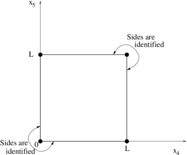
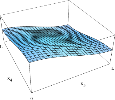
Figure 1: Chiral square compactification (left) and level-1 KK function $f_{0}^{({\bf 1})}(x_{4},x^{5})$ for standard model fields (right).

Equality of the Lagrangian densities on adjacent sides of the square is achieved by enforcing that bulk fields and their first derivatives vary smoothly across the boundary. Applying these boundary conditions to solve the 6D equations of motion for these fields, by separation of variables, we find that the dependence on $x_{4}$ and $x_{5}$ can be expressed in terms of one of four complete and orthonormal sets of functions $f_{n}^{(j,k)}$ with $n=0,1,2,3$, where the KK numbers $(j,k)$ are integers and $j\geq 1$, $k\geq 0$ or $j=k=0$. All $(j,k)$ modes have tree-level mass $\sqrt{j^{2}+k^{2}}/R$ before electroweak symmetry breaking.

2.1 Interactions of the (1,0) modes

We are primarily interested in the phenomenology of the $(1,0)$ modes here. We loosely refer to these as ‘level-1’ modes because they are the lightest nonzero KK modes. For notational brevity we will label them using the superscript ${({\bf 1})}$.

The level-1 KK modes belonging to a tower that includes a zero mode has a KK function

$$f^{({\bf 1})}_{0}(x_{4},x_{5})=\cos{\left(\frac{x_{4}}{R}\right)}+\cos{\left(\frac{x_{5}}{R}\right)}~{},$$ (1)

which is plotted in Figure 1. This is the case for the KK modes of all spin-1 fields and fermions of the same chirality as the observed quarks and leptons, as well as the Higgs doublet. The spinless adjoint field, $A^{({\bf 1})}_{H}$, which is the uneaten combination of the extra-dimensional polarizations of the 6D gauge field, is associated with a KK function which is independent of $x_{4}$,

$$f^{({\bf 1})}_{H}=-\frac{1}{2}\left[f^{({\bf 1})}_{1}(x_{4},x_{5})-f^{({\bf 1})}_{3}(x_{4},x_{5})\right]=-\sin{\frac{x_{5}}{R}}~{},$$ (2)

while the longitudinal component of the vector KK modes is associated with a KK function which is independent of $x_{5}$:

$$f^{({\bf 1})}_{G}=-\frac{i}{2}\left[f^{({\bf 1})}_{1}(x_{4},x_{5})+f^{({\bf 1})}_{3}(x_{4},x_{5})\right]=\sin{\frac{x_{4}}{R}}~{}.$$ (3)

KK modes of fermions come in vectorlike pairs with the component of 4D chirality opposite to the corresponding standard model fermion having KK function $f_{1}$ or $f_{3}$, depending on the 6D chirality.

Integrating over the extra dimensional coordinates gives the 4D effective Lagrangian, which contains kinetic and interaction terms for all SM particles and their KK modes. We limit ourselves to detailing in this section only the couplings of the standard model fields with the level-1 KK modes; the latter are odd under KK parity and so only appear in pairs. The general Lagrangian for all modes is derived in Ref. [6, 7], while the couplings for all fermion modes can be found in Appendix B.

The $SU(3)_{c}$ gauge interactions include the following tree-level couplings between zero modes and $(1,0)$ modes:

$$\mathcal{L}_{\rm gauge} \supset g_{s}f^{abc}\left[G_{\mu}^{{({\bf 1})}a}\left(\partial^{\mu}G^{\nu{({\bf 1})}b}-\partial^{\nu}G^{\mu{({\bf 1})}b}\right)G_{\nu}^{{({\bf 1})}c}-G_{\mu}^{{({\bf 1})}a}G_{\nu}^{{({\bf 1})}b}\partial^{\mu}G^{\nu c}+G_{H}^{{({\bf 1})}a}\partial^{\mu}G_{H}^{{({\bf 1})}b}G_{\mu}^{c}\right]$$ (4)

$$- \frac{g_{s}^{2}}{2}\left[f^{abd}f^{ace}G_{\mu}^{{({\bf 1})}b}G^{\mu{({\bf 1})}c}G_{\nu}^{d}G^{\nu e}+\left(f^{abc}f^{ade}+f^{adc}f^{abe}\right)G_{\mu}^{{({\bf 1})}b}G^{\mu d}G_{\nu}^{{({\bf 1})}c}G^{\nu e}\right]$$

$$+ \frac{g_{s}^{2}}{2}f^{abc}f^{ade}G_{H}^{{({\bf 1})}c}G_{H}^{{({\bf 1})}e}G_{\mu}^{b}G^{\mu d}~{},$$

where $g_{s}$ is the QCD gauge coupling, $f^{abc}$ are the $SU(3)_{c}$ structure constants, and $G_{\mu}^{({\bf 1})}$ and $G_{H}^{({\bf 1})}$ are the level-1 vector and spinless adjoint KK modes of the gluon $G_{\mu}$. We have suppressed all superscripts for zero modes. There are also interactions of the quark modes with the QCD vector and spinless modes:

$$\mathcal{L}_{\rm matter}\supset\!\!\!\displaystyle\sum_{\rm fermions}\!\!\!g_{s}\overline{Q}_{\pm}^{({\bf 1})}G_{\mu}^{a}T^{a}\gamma^{\mu}Q^{({\bf 1})}_{\pm}+g_{s}\bigg{[}\overline{Q}_{\pm}^{({\bf 1})}G_{\mu}^{{({\bf 1})}a}T^{a}\gamma^{\mu}P_{\begin{subarray}{c}L\\ R\end{subarray}}Q_{\pm}-i\overline{Q}_{\pm}^{({\bf 1})}G_{H}^{{({\bf 1})}a}T^{a}P_{\begin{subarray}{c}L\\ R\end{subarray}}Q_{\pm}+{\rm H.c.}\bigg{]}~{},$$ (5)

where fermions with 6D chirality $+$ contain left-handed zero modes, and fermions with 6D chirality $-$ contain right-handed zero modes. The $SU(2)_{W}$ and $U(1)_{Y}$ sectors are analogous, with all the gauge self-couplings set to zero in the Abelian case. The Higgs and ghost terms are given in Ref. [6, 7].

2.2 Mass corrections

Computing radiative corrections in this theory involves taking sums over KK modes, or momenta in the extra dimensions, which fourier transform to operators localized at the corners of the chiral square, $(0,0)$, $(\pi R,\pi R)$ and $(0,\pi R)\sim(\pi R,0)$. The most general 4D effective Lagrangian must therefore allow for these  [14]:

$$L_{eff}=\int_{0}^{L}dx^{4}\int_{0}^{L}dx^{5}\left[\mathcal{L}_{\rm bulk}+\bigg{(}\delta(x_{4})\delta(x_{5})+\delta(L-x_{4})\delta(L-x_{5})\bigg{)}\mathcal{L}_{1}+\delta(L-x_{5})\mathcal{L}_{2}\right]~{},$$ (6)

where $\mathcal{L}_{1}$ and $\mathcal{L}_{2}$ contain all localized operators. Note that KK parity ensures the equality of the operators localized at $(0,0)$ and $(L,L)$. Local operators break 6D Lorentz invariance and hence give rise to mass corrections for KK particles. Such terms are important for models of flat extra dimensions since they allow for the decays of higher modes into pairs of lower ones, a process which would otherwise be on threshold at best due to the quantization of KK mode masses. They also make for a more interesting phenomenology by lifting the degeneracy of states at each level.

The localized terms contain contributions from ultraviolet physics as well as from running down from the cut-off. Being unable to compute the former, we assume that they are generically smaller than the logarithmically-enhanced one-loop terms which are calculable (for further discussion see [14, 12]). Level-1 fermions acquire the following mass corrections  [5]:

$$\delta(M_{Q_{+}}) = \left(\frac{16}{3}g_{s}^{2}+3g^{2}+\frac{1}{9}g^{\prime 2}+\frac{5}{8}\lambda_{Q_{+}}^{2}\right)\frac{l_{0}}{R}+\frac{1}{2}m_{q}^{2}R~{},$$

$$\delta(M_{Q_{-}}) = \left(\frac{16}{3}g_{s}^{2}+4g^{\prime 2}y^{2}+\frac{10}{8}\lambda_{Q_{-}}^{2}\right)\frac{l_{0}}{R}+\frac{1}{2}m_{q}^{2}R~{},$$

$$\delta(M_{L_{+}}) = \left(3g^{2}+g^{\prime 2}\right)\frac{l_{0}}{R}~{},$$

$$\delta(M_{E_{-}}) = \frac{g^{\prime 2}}{4\pi^{2}}\frac{l_{0}}{R}~{},$$ (7)

where $g_{s}$, $g$ and $g^{\prime}$ are the $SU(3)_{c}\times SU(2)_{W}\times U(1)_{Y}$ gauge couplings, $\lambda_{Q_{\pm}}$ are the Yukawa couplings of $Q_{\pm}$ to the Higgs doublet, and $l_{0}$ is a common loop factor,

$$l_{0}=\frac{1}{16\pi^{2}}\ln\left(\Lambda R\right)^{2}~{}.$$ (8)

An estimate of the cutoff of the effective theory, based on naive dimensional analysis, gives $\Lambda\approx 10/R$ [5]. The terms linear in $R$ shown in Eq. (7) are small corrections to the tree-level masses due to electroweak symmetry breaking masses, $m_{q}$.

The (1,0) vector bosons also receive radiative corrections to their masses,

$$\delta M_{G_{\mu}^{({\bf 1})}} = 4g_{s}^{2}\frac{l_{0}}{R}~{},$$

$$\delta M_{W_{\mu}^{({\bf 1})}} = \frac{123}{24}g^{2}\frac{l_{0}}{R}~{},$$

$$\delta M_{B_{\mu}^{({\bf 1})}} = -\frac{165}{24}g^{\prime 2}\frac{l_{0}}{R}~{},$$ (9)

while only the spinless adjoints in the electroweak sector have mass corrections:

$$\delta M_{G_{H}^{({\bf 1})}} = 0$$

$$\delta M_{W_{H}^{({\bf 1})}} = -\frac{51}{8}g^{2}\frac{l_{0}}{R}+\frac{m_{W}^{2}R}{2}~{},$$

$$\delta M_{B_{H}^{({\bf 1})}} = -\frac{307}{8}g^{\prime 2}\frac{l_{0}}{R}~{}.$$ (10)

The above mass shifts include negative contributions from fermions in loops, allowing for overall negative corrections to masses. This is especially important when there are no self-interactions to compete with the fermion interactions, as is the case with for the hypercharge bosons.

boson	$MR$	fermion	$MR$
$G_{\mu}^{({\bf 1})}$	1.392	$Q_{+}^{{({\bf 1})}3}$	$\!1.265+\frac{1}{2}(m_{t}R)^{2}\!$
$\!W_{\mu}^{({\bf 1})}$	$1.063+\frac{1}{2}(M_{W}R)^{2}\!$	$T_{-}^{({\bf 1})}$	$\!1.252+\frac{1}{2}(m_{t}R)^{2}\!$
$G_{H}^{({\bf 1})}$	1.0	$Q_{+}^{({\bf 1})}$	1.247
$B_{\mu}^{({\bf 1})}$	0.974	$U_{-}^{({\bf 1})}$	1.216
$\!W_{H}^{({\bf 1})}$	$0.921+\frac{1}{2}(m_{W}R)^{2}\!$	$D_{-}^{({\bf 1})}$	1.211
$B_{H}^{({\bf 1})}$	0.855	$L_{+}^{({\bf 1})}$	1.041
		$E_{-}^{({\bf 1})}$	1.015

Table 1: Masses of the (1,0) particles in $1/R$ units (left). The (1,0) Higgs particles are not included here because their masses are quadratically sensitive to the cutoff scale. The right-hand panel shows the spectrum for $1/R=0.5$ TeV.

The masses of the (1,0) particles are given in Table 1 in units of $1/R$. The mass shifts are evaluated there for gauge couplings $g_{s}=1.16$, $g=0.65$ and $g^{\prime}=0.36$, which are the values obtained using the standard model one-loop running up to the scale $1/R=500$ GeV, We will use the masses from Table 1 throughout the paper, ignoring further running of the gauge couplings above 500 GeV (note that the standard model running of the gauge couplings between 500 GeV and 1 TeV results in only a 3% change in $g_{s}$ and negligible changes in $g$ and $g^{\prime}$; however, above $\sim 1/R$ the running is accelerated by the presence of the level-1 modes).

The KK modes of the Higgs doublet have mass-squared shifts which are quadratically sensitive to the cutoff scale $\Lambda$ [12]. Hence, the masses of the (1,0) Higgs scalars may be treated as free parameters (determined by the underlying theory above $\Lambda$, which is not specified in our framework). Furthermore, additional structures such as the Twin Higgs mechanism [15] may be used to cancel the quadratic divergences in models with universal extra dimensions [16], potentially affecting the (1,0) Higgs sector. We assume here that the (1,0) Higgs particles are heavier than $1/R$. In that case, the hadron collider phenomenology is mostly independent of the exact (1,0) Higgs masses.

2.3 Loop-induced bosonic operators

In addition to lifting the degeneracy of the $(1,0)$ masses, loop corrections also contribute to the following dimension-5 operators that are of particular interest for computing the branching fractions of the $(1,0)$ bosons:

$$-\frac{R}{4}\Big{(}\mathcal{C}_{B}\epsilon^{\mu\nu\alpha\beta}F_{\mu\nu}B^{({\bf 1})}_{\alpha\beta}B_{H}^{({\bf 1})}+\mathcal{C}_{G}\epsilon^{\mu\nu\alpha\beta}G_{\mu\nu}B^{({\bf 1})}_{\alpha\beta}G_{H}^{({\bf 1})}\Big{)}~{},$$ (11)

where $F_{\mu\nu}$ and $G_{\mu\nu}$ are the field strengths of the photon and gluon, respectively, $B^{({\bf 1})}_{\alpha\beta}$ is the field strength of the $(1,0)$ hypercharge vector boson $B^{({\bf 1})}_{\alpha}$, and $B_{H}^{({\bf 1})}$ is the $U(1)_{Y}$ spinless adjoint. These operators account for the only significant 2-body decay channels open to the level-1 KK modes $G^{({\bf 1})}_{H}$ and $B^{({\bf 1})}_{\mu}$. The analogous operator with the photon replaced by the $Z$ boson is less relevant because the corresponding decay width is phase-space suppressed. The coefficients of the above dimension-5 operators are computed in Appendix B, with the result:

$$\mathcal{C}_{B}=\frac{g^{\prime 2}e}{8\pi^{2}R}\frac{1}{M_{B_{\nu}^{({\bf 1})}}^{2}-M_{B_{H}^{({\bf 1})}}^{2}}\sum_{F}\sigma_{F}\Big{(}\frac{Y_{F}}{2}\Big{)}^{2}Q_{F}{\cal E}_{F}~{},$$ (12)

where $\sigma_{F}=\pm 1$ for a 6D fermion $F$ of chirality $\pm$, $Q_{F}$ is the electric charge, $Y_{F}$ is the hypercharge normalized to be twice the electric charge for $SU(2)_{W}$ singlets and ${\cal E}_{F}$ is a function of the masses of $B_{H}^{({\bf 1})}$, $B_{\nu}^{({\bf 1})}$, and of the (1,0) and (1,1) fermions given in Eq. (B.10). $\mathcal{C}_{G}$ is given by an analogous expression, but it is suppressed by the small mass difference between the initial- and final-state $(1,0)$ bosons.

One might also naively expect higher-dimension operators of the form

$$G_{\mu\nu}\partial^{\mu}B_{H}^{({\bf 1})}\partial^{\nu}G_{H}^{({\bf 1})}+Z_{\mu\nu}\partial^{\mu}B_{H}^{({\bf 1})}\partial^{\nu}W_{H}^{{({\bf 1})}3}+\left(W_{\mu\nu}^{+}\partial^{\mu}B_{H}^{({\bf 1})}\partial^{\nu}W_{H}^{{({\bf 1})}-}+{\rm H.c.}\right)~{},$$ (13)

to be generated, where $W^{({\bf 1})}_{H}$ is the level-1 $SU(2)_{W}$ spinless adjoint and $W_{\mu\nu}$ and $Z_{\mu\nu}$ are the standard model field strengths for the $W$ and $Z$ bosons. However, the first of these terms is identically zero as can be seen after integrating by parts and using the gluon field equation. By the same method one can see that the coefficients of the last two terms are small, being proportional to $(m_{W}R)^{2}$, and furthermore the resulting decay widths for $W_{H}^{{({\bf 1})}}$ are also phase-space suppressed.

3 Decays of the level-1 particles

KK parity allows any (1,0) particle to decay only into a lighter (1,0) particle and one or more standard model particles. The lightest (1,0) particle is stable. In this section we compute the branching fractions of the (1,0) particles assuming that the generic features of the ‘one-loop’ mass spectrum, shown in Table 1, are not modified by higher-order corrections.

3.1 Color-singlet $(1,0)$ particles

The $W^{{({\bf 1})}}_{H}$ boson (the spinless adjoint of $SU(2)_{W}$) is the next-to-lightest (1,0) particle, and therefore can decay only into a $B^{{({\bf 1})}}_{H}$ plus standard model particles. The dominant decay mode of its electrically neutral component is the 3-body decay $W^{{({\bf 1})}3}_{H}\to B^{{({\bf 1})}}_{H}l\bar{l}$, where $l$ are leptons. The width for this decay, computed in Appendix C, is given by

$$\Gamma\left(W^{{({\bf 1})}3}_{H}\to B^{{({\bf 1})}}_{H}e^{+}e^{-}\right)=\,\frac{\alpha^{2}\,M_{W_{H}^{{({\bf 1})}}}}{128\pi\cos^{2}\!\theta_{w}\,\sin^{2}\!\theta_{w}}\,{\cal I}_{+}\!\left(M_{W_{H}^{({\bf 1})}},M_{B_{H}^{({\bf 1})}},M_{L_{+}^{({\bf 1})}}\right)~{},$$ (1)

and is the same for any lepton pair. The dimensionless function ${\cal I}_{+}$ contains phase space integrals for the decay and is defined in Eq. (C.8). Expanding this to leading order in the mass difference $M_{W_{H}^{({\bf 1})}}-M_{B_{H}^{({\bf 1})}}$, which is accurate to about 25% for the mass spectrum in Table 1 [see Eq. (C.18) in Appendix C], we find that the width of the $W^{{({\bf 1})}3}_{H}$ decay into $B^{{({\bf 1})}}_{H}$ plus quarks has a simple expression in terms of the decay width into $B^{{({\bf 1})}}_{H}$ plus leptons:

$$\Gamma\left(W^{{({\bf 1})}3}_{H}\to B^{{({\bf 1})}}_{H}q\overline{q}\right)\approx\frac{1}{3}\left(\frac{M_{L_{+}^{{({\bf 1})}}}^{2}-M^{2}_{W_{H}^{{({\bf 1})}}}}{M_{Q_{+}^{{({\bf 1})}}}^{2}-M^{2}_{W_{H}^{{({\bf 1})}}}}\right)^{\!\!4}\Gamma\left(W^{{({\bf 1})}}_{H}\to B^{{({\bf 1})}}_{H}e^{+}e^{-}\right)~{},$$ (2)

where we have not summed over quark flavors. Given that $W_{H}^{{({\bf 1})}}$ is closer to $L_{+}^{{({\bf 1})}}$ in mass than to $Q_{+}^{{({\bf 1})}}$, it follows that the decay into quarks is highly suppressed. The ensuing branching fractions for the $W_{H}^{{({\bf 1})}\,3}\to B^{{({\bf 1})}}_{H}$ transition are approximately 1/6 for each of the $e^{+}e^{-}$, $\mu^{+}\mu^{-}$ and $\tau^{+}\tau^{-}$ final states, 1/2 for $\nu\overline{\nu}$, and $0.5$% for the sum of all quark-antiquark pairs.

The electrically charged spinless adjoints of $SU(2)_{W}$, $W_{H}^{{({\bf 1})}\,\pm}$, decay with a branching fraction of nearly 1/3 into each of the $e^{\pm}\nu B^{{({\bf 1})}}_{H}$, $\mu^{\pm}\nu B^{{({\bf 1})}}_{H}$ and $\tau^{\pm}\nu B^{{({\bf 1})}}_{H}$ final states, while the branching fraction into $q\overline{q}B^{{({\bf 1})}}_{H}$ is again negligible.

The spin-1 boson $B^{{({\bf 1})}}_{\mu}$ may decay only into a $B^{{({\bf 1})}}_{H}$ or $W^{{({\bf 1})}}_{H}$ and standard model particles. An important tree-level decay is into right-handed leptons and a $B^{{({\bf 1})}}_{H}$, with a width:

$$\Gamma\left(B^{({\bf 1})}_{\mu}\to B^{{({\bf 1})}}_{H}e_{R}^{+}e_{R}^{-}\right)=\frac{\alpha^{2}M_{E_{-}^{{({\bf 1})}}}^{2}}{24\pi\cos^{4}\!\theta_{w}\,M_{B_{\mu}^{({\bf 1})}}}\,{\cal I}_{-}\!\left(M_{B_{\mu}^{({\bf 1})}},M_{B_{H}^{({\bf 1})}},M_{E_{-}^{({\bf 1})}}\right)~{},$$ (3)

where ${\cal I}_{-}$ is another phase space integral defined in Eq. (C.8). The width into left-handed leptons,

$$\Gamma\left(B^{{({\bf 1})}}_{\mu}\to B^{{({\bf 1})}}_{H}e_{L}^{+}e_{L}^{-}\right)=\frac{\alpha^{2}M_{L_{+}^{{({\bf 1})}}}^{2}}{384\pi\cos^{4}\!\theta_{w}\,M_{B_{\mu}^{({\bf 1})}}}\,{\cal I}_{-}\!\left(M_{B_{\mu}^{({\bf 1})}},M_{B_{H}^{({\bf 1})}},M_{L_{+}^{({\bf 1})}}\right)~{},$$ (4)

is suppressed due to the smaller hypercharge and larger mass of the (1,0) fermion, which is $L_{+}^{({\bf 1})}$ in this case. For the same reasons, the $B^{{({\bf 1})}}_{\mu}$ decay into a $B^{{({\bf 1})}}_{H}$ and $q\overline{q}$ pairs has a small decay width. $B^{{({\bf 1})}}_{\mu}$ decays to $W^{{({\bf 1})}}_{H}$ plus fermion pairs are highly suppressed due to the dependence on the 7th power of the small difference between initial and final (1,0) masses [see Eqs. (C.12) and (C.18) in Appendix C].

Besides these tree-level 3-body decays, $B^{{({\bf 1})}}_{\mu}$ also has 2-body decays via the dimension-5 operator shown in Eq. (11), which is induced at one loop (see Appendix B). The decay width is given by

$$\Gamma\left(B^{{({\bf 1})}}_{\mu}\to B^{{({\bf 1})}}_{H}\gamma\right)=\frac{\alpha^{3}}{96\pi^{2}\cos^{4}\!\theta_{w}}\frac{1}{M_{B_{\mu}^{({\bf 1})}}}\left(1-\frac{M_{B_{H}^{({\bf 1})}}^{2}}{M_{B_{\mu}^{({\bf 1})}}^{2}}\right)\left(\sum_{F}\sigma_{F}\,\Big{(}\frac{Y_{F}}{2}\Big{)}^{2}\,Q_{F}\,{\cal E}_{F}\right)^{2}~{},$$ (5)

where the sum over $F$ includes all quarks and leptons, $\sigma_{F}$ is +1 for $SU(2)_{W}$ doublets and $-1$ for $SU(2)_{W}$ singlets, $Q_{F}$ is the electric charge, $Y_{F}$ is the hypercharge normalized to be twice the electric charge for $SU(2)_{W}$ singlets, and ${\cal E}_{F}$ is given in Eq. (B.10) and depends only on the masses of $B_{H}^{({\bf 1})}$, $B_{\nu}^{({\bf 1})}$, and of the (1,0) and (1,1) fermions. Using the values for the standard model gauge couplings given at the end of section 2.2, i.e., $\alpha=1/127$ and $\sin^{2}\!\theta_{w}=0.235$, we find the following branching fractions for $B^{{({\bf 1})}}_{\mu}$:

$${\rm Br}\left(B^{{({\bf 1})}}_{\mu}\rightarrow B^{{({\bf 1})}}_{H}\gamma\right)\equiv b_{B\gamma}\approx 34.0\%~{},$$

$${\rm Br}\left(B^{{({\bf 1})}}_{\mu}\rightarrow B^{{({\bf 1})}}_{H}e^{+}e^{-}\right)\equiv b_{Be}\approx 21.3\%~{}.$$ (6)

The branching fractions into $e^{+}e^{-}B^{{({\bf 1})}}_{H}$, $\mu^{+}\mu^{-}B^{{({\bf 1})}}_{H}$ and $\tau^{+}\tau^{-}B^{{({\bf 1})}}_{H}$ are equal. The fact that the tree-level 3-body decay and the one-loop 2-body decay have comparable branching fractions in the case of $B^{{({\bf 1})}}_{\mu}$ is an accidental consequence of the mass spectrum given in Table 1. The $B^{{({\bf 1})}}_{\mu}$ decays into $B^{{({\bf 1})}}_{H}$ plus neutrinos or quarks have small branching fractions (1.4% and 0.6%, respectively) which may be safely ignored in what follows.

The (1,0) leptons can decay into (1,0) modes of the electroweak gauge bosons or spinless adjoints, and a standard model lepton. The decay widths of the $SU(2)_{W}$-doublet (1,0) leptons, $L_{+}^{{({\bf 1})}}\equiv(N_{+}^{{({\bf 1})}},E_{+}^{{({\bf 1})}})$, to neutral (1,0) particles are given at tree level by:

$$\Gamma\left(L_{+}^{{({\bf 1})}}\!\to W_{H}^{{({\bf 1})}3}l_{L}\right) \!=\! \frac{\alpha}{32\sin^{2}\!\theta_{w}}M_{L^{{({\bf 1})}}}\left(1-\frac{M_{W_{H}^{{({\bf 1})}}}^{2}}{M_{L^{{({\bf 1})}}}^{2}}\right)^{\!2}~{},$$

$$\hskip 0.28453pt\Gamma\left(L_{+}^{{({\bf 1})}}\!\to B^{{({\bf 1})}}_{\mu}l_{L}\right) \!=\! \frac{\alpha}{16\cos^{2}\!\theta_{w}}M_{L^{{({\bf 1})}}}\left(1-\frac{M_{B_{\mu}^{{({\bf 1})}}}^{2}}{M_{L^{{({\bf 1})}}}^{2}}\right)^{\!2}\left(1+\frac{M_{L^{{({\bf 1})}}}^{2}}{2M_{B_{\mu}^{{({\bf 1})}}}^{2}}\right)~{},$$

$$\hskip 0.28453pt\Gamma\left(L_{+}^{{({\bf 1})}}\!\to B_{H}^{{({\bf 1})}}l_{L}\right) \!=\! \frac{\alpha}{32\cos^{2}\!\theta_{w}}M_{L^{{({\bf 1})}}}\left(1-\frac{M_{B_{H}^{{({\bf 1})}}}^{2}}{M_{L^{{({\bf 1})}}}^{2}}\right)^{\!2}\,,$$ (7)

where $l_{L}$ is the corresponding standard model weak doublet lepton. The decays to charged (1,0) particles, $E_{+}^{{({\bf 1})}}\!\to W_{H}^{{({\bf 1})}-}\nu_{L}$ and $N_{+}^{{({\bf 1})}}\!\to W_{H}^{{({\bf 1})}-}e_{L}^{+}$, have a width twice as large as the $L_{+}^{{({\bf 1})}}\!\to W_{H}^{{({\bf 1})}3}l_{L}$ decay width. The $L_{+}^{{({\bf 1})}}$ branching fractions are given by:

$${\rm Br}\left[(N_{+}^{{({\bf 1})}},E_{+}^{{({\bf 1})}})\to B_{H}^{{({\bf 1})}}(\nu_{L},e_{L})\right]\equiv b_{l1}\approx 20.1\%~{}.$$

$$\frac{1}{2}\,{\rm Br}\left[(N_{+}^{{({\bf 1})}},E_{+}^{{({\bf 1})}})\to W_{H}^{{({\bf 1})}+}(e_{L},\nu_{L})\right]={\rm Br}\left[(N_{+}^{{({\bf 1})}},E_{+}^{{({\bf 1})}})\to W_{H}^{{({\bf 1})}3}(\nu_{L},e_{L})\right]\equiv b_{l2}\approx 23.5\%~{},$$

$${\rm Br}\left[(N_{+}^{{({\bf 1})}},E_{+}^{{({\bf 1})}})\to B_{\mu}^{{({\bf 1})}}(\nu_{L},e_{L})\right]\equiv b_{l3}\approx 9.3\%~{}.$$ (8)

Final-state	$W_{\mu}^{{({\bf 1})}3}\!\to...\to B_{H}^{{({\bf 1})}}$			Final-state	$W_{\mu}^{{({\bf 1})}+}\!\to...\to B_{H}^{{({\bf 1})}}$
$e,\mu,\gamma$	Branching fractions	%		$e,\mu,\gamma$	Branching fractions	%
$X$	$\frac{\textstyle 2}{\textstyle 3}(b_{l1}+b_{l2}+b_{l3}b_{Be})$	30.4		$X$	$\frac{\textstyle 1}{\textstyle 3}(b_{l1}+2b_{l2}+b_{l3}b_{Be})$	23.1
$(e^{+}+e^{-})X$	$\frac{\textstyle 4}{\textstyle 9}b_{l2}$	10.5		$e^{+}\,X$	$\frac{\textstyle 1}{\textstyle 3}(b_{l1}+2b_{l2}+b_{l3}b_{Be})$	23.1
$\!(e^{+}\!\mu^{-}\!\!+e^{-}\!\mu^{+})X\!\!$	$\frac{\textstyle 4}{\textstyle 9}b_{l2}$	10.5		$e^{+}e^{-}\,X$	$\frac{\textstyle 1}{\textstyle 6}(b_{l2}+2b_{l3}b_{Be})$	4.6
$e^{+}e^{-}\,X$	$\frac{\textstyle b_{l1}}{\textstyle 6}+\frac{\textstyle 4}{\textstyle 9}b_{l2}+\frac{\textstyle 5}{\textstyle 6}b_{l3}b_{Be}\!$	15.5		$\!e^{+}e^{-}e^{+}X\!$	$\frac{\textstyle 1}{\textstyle 6}(b_{l2}+2b_{l3}b_{Be})$	4.6
$e^{+}e^{-}e^{+}e^{-}$	$\frac{\textstyle 1}{\textstyle 36}(b_{l2}+6b_{l3}b_{Be})$	1.0		$\!e^{+}e^{-}\mu^{+}X\!$	$\frac{\textstyle 1}{\textstyle 6}(b_{l2}+2b_{l3}b_{Be})$	4.6
$\!e^{+}e^{-}\mu^{+}\mu^{-}$	$\frac{\textstyle 1}{\textstyle 18}(b_{l2}+6b_{l3}b_{Be})$	2.0		$\gamma\,X$	$\frac{\textstyle 1}{\textstyle 3}b_{l3}b_{B\gamma}$	1.1
$\gamma\,X$	$\frac{\textstyle 2}{\textstyle 3}b_{l3}b_{B\gamma}$	2.1		$\gamma\;e^{+}\,X$	$\frac{\textstyle 1}{\textstyle 3}b_{l3}b_{B\gamma}$	1.1
$\gamma\;e^{+}e^{-}\,X$	$\frac{\textstyle 1}{\textstyle 6}b_{l3}b_{B\gamma}$	0.5

Table 2: Branching fractions for the complete cascade decays of $W_{\mu}^{{({\bf 1})}3}$ and $W_{\mu}^{{({\bf 1})}+}$. $X$ stands for a number of neutrinos or taus. The branching fractions involving more muons than electrons (not shown) are equal to the analogous ones involving more electrons than muons. The branching fractions of $W_{\mu}^{{({\bf 1})}-}$ are the same as for $W_{\mu}^{{({\bf 1})}+}$ except for flipping the electric charges of the final state leptons. The branching fractions for ‘one-step’ decays, $b_{l1}$, $b_{l2}$, $b_{l3}$ and $b_{Be}$, $b_{B\gamma}$, are defined in Eqs. (8) and (6).

As opposed to the three spinless adjoints and $B_{\mu}^{{({\bf 1})}}$ which at tree level have only 3-body decays, the $W_{\mu}^{{({\bf 1})}}$ particles are heavier than the (1,0) leptons and therefore decay with a branching fraction of almost 100% into one (1,0) lepton doublet and the corresponding standard model lepton doublet. Putting together the branching fractions for various decays of the electroweak (1,0) bosons, we find the branching fractions for the complete cascade decays of $W_{\mu}^{{({\bf 1})}3}$ shown in Table 2.

3.2 Colored (1,0) particles

At tree level, the (1,0) spinless adjoint of $SU(3)_{c}$ has only 3-body decays into a quark-antiquark pair and one of the electroweak (1,0) bosons. The decay widths are derived in Appendix C, and take the following form:

$$\Gamma\left(G^{{({\bf 1})}}_{H}\to B^{{({\bf 1})}}_{H}u_{R}\overline{u}_{R}\right)=\frac{y_{u_{R}}^{2}\alpha\alpha_{s}}{64\pi\cos^{2}\!\theta_{w}}\,M_{G_{H}^{{({\bf 1})}}}\,{\cal I}_{+}\!\left(M_{G_{H}^{({\bf 1})}},M_{B_{H}^{({\bf 1})}},M_{U_{-}^{({\bf 1})}}\right)~{},$$ (9)

$$\Gamma\left(G^{{({\bf 1})}}_{H}\to B^{{({\bf 1})}}_{\mu}u_{R}\overline{u}_{R}\right)\approx\frac{y_{u_{R}}^{2}\alpha\alpha_{s}}{140\pi\cos^{2}\!\theta_{w}}\,M_{G_{H}^{{({\bf 1})}}}\,\frac{M_{U_{-}^{{({\bf 1})}}}^{2}}{M_{B_{\mu}^{{({\bf 1})}}}^{2}}\frac{\left(M_{G_{H}^{{({\bf 1})}}}-M_{B_{\mu}^{{({\bf 1})}}}\right)^{7}}{(M_{U_{-}^{{({\bf 1})}}}^{2}-M^{2}_{G_{H}^{{({\bf 1})}}})^{4}}~{},$$ (10)

for hypercharge (1,0) bosons in the final state, and

$$\Gamma\left(G^{{({\bf 1})}}_{H}\to W^{{({\bf 1})}3}_{H}u_{L}\overline{u}_{L}\right) \approx \frac{\alpha\alpha_{s}}{420\pi\sin^{2}\!\theta_{w}}\,M_{G_{H}^{{({\bf 1})}}}^{2}\frac{\left(M_{G_{H}^{{({\bf 1})}}}-M_{W_{H}^{{({\bf 1})}}}\right)^{7}}{(M_{Q_{+}^{{({\bf 1})}}}^{2}-M^{2}_{G_{H}^{{({\bf 1})}}})^{4}}~{},$$

$$\Gamma\left(G^{{({\bf 1})}}_{H}\to W^{{({\bf 1})}+}_{H}d_{L}\overline{u}_{L}\right) = \Gamma\left(G^{{({\bf 1})}}_{H}\to W^{{({\bf 1})}-}_{H}u_{L}\overline{d}_{L}\right)=2\,\Gamma\left(G^{{({\bf 1})}}_{H}\to W^{{({\bf 1})}3}_{H}u_{L}\overline{u}_{L}\right)~{},$$ (11)

for $SU(2)_{W}$ (1,0) bosons. Note that we have expanded the decay widths to leading order in the mass difference of $G_{H}^{{({\bf 1})}}$ and the electroweak (1,0) boson [see Eq. (C.18)] in the case of $G_{H}\to B_{\mu}$ and $G_{H}\to W_{H}$ transitions, but not for $G_{H}\to B_{H}$ where the mass difference is larger and the expansion does not provide a good approximation.

$G^{{({\bf 1})}}_{H}$ has also a two-body decay into $B^{{({\bf 1})}}_{\mu}$ and a gluon, via a dimension-5 operator shown in Eq. (11), which is induced at one loop. However, the width for this decay is highly suppressed because $G^{{({\bf 1})}}_{H}$ and $B^{{({\bf 1})}}_{\mu}$ are almost degenerate.

After summing over all quark flavors, we find that the dominant decay mode of $G^{{({\bf 1})}}_{H}$ is into $B^{{({\bf 1})}}_{H}q\overline{q}$, with a total branching fraction of $b_{g1}\approx 96.5\%$. The sum over all branching fractions of $G^{{({\bf 1})}}_{H}$ into $W^{{({\bf 1})}+}_{H}$ or $W^{{({\bf 1})}-}_{H}$ plus a quark-antiquark pair is $b_{g2}^{\prime}\approx 2.3\%$. The branching fraction for $G^{{({\bf 1})}}_{H}\to W^{{({\bf 1})}3}_{H}q\overline{q}$ is $b_{g2}\approx 1.2\%$, while the decay into $B_{\mu}^{{({\bf 1})}}$ is highly suppressed due to the very small mass difference involved in that case. The branching fractions quoted here correspond to $1/R=500$ GeV. For different values of $1/R$, the branching fractions of $G^{{({\bf 1})}}_{H}$ change slightly due to the dependence of $M_{T_{\pm}^{({\bf 1})}}R$ on $1/R$ shown in Table 1. For the coupling constants we use $\alpha_{s}=0.107$, $\alpha=1/127$ and $\sin^{2}\theta_{w}=0.235$, which are the standard model values at 500 GeV.

The (1,0) quarks can decay into both vector and spinless modes. The largest decay width is into a $G_{H}^{{({\bf 1})}}$ and a standard model quark:

$$\Gamma\left(Q^{{({\bf 1})}}\!\to G_{H}^{{({\bf 1})}}q\right)=\frac{\alpha_{s}}{6}\,M_{Q^{{({\bf 1})}}}\left(1-\frac{M_{G_{H}^{{({\bf 1})}}}^{2}}{M_{Q^{{({\bf 1})}}}^{2}}\right)^{\!2}~{}.$$ (12)

The $SU(2)_{W}$-doublet (1,0) quarks can also decay into a standard-model quark, and an $SU(2)_{W}$ gauge boson or spinless adjoint. Ignoring the standard-model quark mass, the decay width for the latter is

$$\Gamma\left(Q_{+}^{{({\bf 1})}}\!\to W_{H}^{{({\bf 1})}3}q_{L}\right)=\frac{\alpha}{32\sin^{2}\!\theta_{w}}M_{Q_{+}^{{({\bf 1})}}}\left(1-\frac{M_{W_{H}^{{({\bf 1})}}}^{2}}{M_{Q^{{({\bf 1})}}}^{2}}\right)^{\!2}~{},$$ (13)

and is twice as large in the case of $W_{H}^{{({\bf 1})}\pm}$. The decays of (1,0) quarks into an $SU(2)_{W}$ (1,0) vector boson and a standard model quark have a width

$$\Gamma\left(Q^{{({\bf 1})}}_{+}\!\to W^{{({\bf 1})}3}_{\mu}q_{L}\right)=\left(\frac{M_{Q_{+}^{{({\bf 1})}}}^{2}-M_{W_{\mu}^{{({\bf 1})}}}^{2}}{M_{Q_{+}^{{({\bf 1})}}}^{2}-M_{W_{H}^{{({\bf 1})}}}^{2}}\right)^{\!2}\left(2+\frac{M_{Q_{+}^{{({\bf 1})}}}^{2}}{M_{W_{\mu}^{{({\bf 1})}}}^{2}}\right)\Gamma\left(Q_{+}^{{({\bf 1})}}\!\to W_{H}^{{({\bf 1})}3}q_{L}\right)~{}.$$ (14)

The width is twice as large for $Q_{+}^{{({\bf 1})}}\!\to W^{{({\bf 1})}\pm}_{\mu}q_{L}$.

All (1,0) quarks may also decay into (1,0) hypercharge bosons with widths

$$\Gamma\left(Q^{{({\bf 1})}}\!\to B_{H}^{{({\bf 1})}}q\right) \!=\! \frac{Y^{2}_{q}\alpha}{32\cos^{2}\!\theta_{w}}M_{Q^{{({\bf 1})}}}\left(1-\frac{M_{B_{H}^{{({\bf 1})}}}^{2}}{M_{Q^{{({\bf 1})}}}^{2}}\right)^{\!2}~{},$$

$$\Gamma\left(Q^{{({\bf 1})}}\!\to B^{{({\bf 1})}}_{\mu}q\right) \!=\! \left(\frac{M_{Q^{{({\bf 1})}}}^{2}-M_{B_{\mu}^{{({\bf 1})}}}^{2}}{M_{Q^{{({\bf 1})}}}^{2}-M_{B_{H}^{{({\bf 1})}}}^{2}}\right)^{\!2}\left(2+\frac{M_{Q^{{({\bf 1})}}}^{2}}{M_{B_{\mu}^{{({\bf 1})}}}^{2}}\right)\Gamma\left(Q^{{({\bf 1})}}\!\to B_{H}^{{({\bf 1})}}q\right)~{},$$ (15)

where $Y_{q}$ is the hypercharge of the quark $q$, normalized to be 1/3 for $SU(2)_{W}$ doublets. The branching fractions of the (1,0) quarks of the first and second generations are shown in Table 3.

The $B_{-}^{{({\bf 1})}}$ quark has the same branching fractions as $D_{-}^{{({\bf 1})}}$, while those of the $Q_{+}^{{({\bf 1})}3}=(T_{+}^{{({\bf 1})}},B_{+}^{{({\bf 1})}})$ quarks are more sensitive to $1/R$, as shown in Figure 2, because of the large top quark mass. Finally, the KK mode of the $SU(2)_{W}$-singlet top quark, $T_{-}^{{({\bf 1})}}$, has branching fractions highly sensitive to the mass of (1,0) Higgs particles, with the decay into $b\,H^{{({\bf 1})}+}$ dominating over $t\,G_{H}^{({\bf 1})}$ if $H^{{({\bf 1})}+}$ is light. Because of this fact, and also because of their small production cross section, third generation fermions do not result in many multi-lepton events. Hence we will not give an expression for their branching fractions here.

$V^{{({\bf 1})}}$	Br$\left(U_{+}^{{({\bf 1})}}\!\to q_{L}V^{{({\bf 1})}}\!\right)\!$		$V^{{({\bf 1})}}$	Br$\left(U_{-}^{{({\bf 1})}}\!\to u_{R}V^{{({\bf 1})}}\!\right)\!\!$	Br$\left(D_{-}^{{({\bf 1})}}\!\to d_{R}V^{{({\bf 1})}}\!\right)\!\!\!\!$
$G_{H}^{{({\bf 1})}}$	$b_{q3}\approx 63.2\%$		$G_{H}^{{({\bf 1})}}$	$b_{u3}\approx 82.1\%$	$b_{d3}\approx 94.8\%$
$\!\!W_{\mu}^{{({\bf 1})}3}$ ; $W_{\mu}^{{({\bf 1})}+}\!\!$	$b_{q2}\approx 6.4\%$ ; $2b_{q2}$		$B_{\mu}^{{({\bf 1})}}$	$b_{u2}\approx 11.5\%$	$b_{d2}\approx 3.3\%$
$\!\!W_{H}^{{({\bf 1})}3}$ ; $W_{H}^{{({\bf 1})}+}\!\!$	$b_{q1}\approx 5.6\%$ ; $2b_{q1}$		$B_{H}^{{({\bf 1})}}$	$b_{u1}\approx 6.4\%$	$b_{d1}\approx 1.9\%$
$B_{\mu}^{{({\bf 1})}}$	$b_{q0}\approx 0.55\%$

Table 3: Branching fractions of first and second generation (1,0) quarks, in percentage. $D_{+}^{({\bf 1})}$ have the same branching fractions as $U_{+}^{({\bf 1})}$ except for a flip of the electric charge of the (1,0) bosons. The $U_{+}^{({\bf 1})}$ decays into a $B_{H}^{{({\bf 1})}}$ and a quark is not shown because it is too small to be relevant.

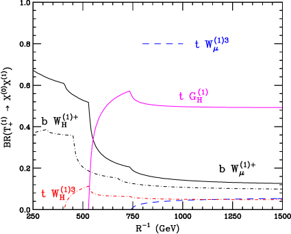
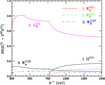
Figure 2: Branching fractions for the $SU(2)_{W}$-doublet (1,0) quarks of the third generation, assuming that the (1,0) Higgs particles have a mass $M_{H^{({\bf 1})}}=1.05/R$.

The (1,0) vector gluon decays into a standard model quark and a (1,0) quark. The width in the case of $SU(2)_{W}$-singlet down-type quarks is given by

$$\Gamma\left(G_{\mu}^{{({\bf 1})}}\!\rightarrow\sum_{i=1,2,3}D_{-_{R}}^{{({\bf 1})}i}d_{R}^{i}\right)=\frac{\alpha_{s}}{2}M_{G_{\mu}^{{({\bf 1})}}}\left(1-\frac{M_{D_{-}^{{({\bf 1})}}}^{2}}{M_{G_{\mu}^{{({\bf 1})}}}^{2}}\right)^{\!2}\left(1+\frac{M_{D_{-}^{{({\bf 1})}}}^{2}}{2M_{G_{\mu}^{{({\bf 1})}}}^{2}}\right)~{}.$$ (16)

The widths into all other (1,0) quarks except for the top have similar forms. For $1/R\begin{array}[]{c}\,\sim\vspace{-21pt}\\ <\end{array}1.3$ TeV the decays of the (1,0) vector gluon into $t_{L}T_{+_{L}}^{{({\bf 1})}}$ or $t_{R}T_{-_{R}}^{{({\bf 1})}}$ have a highly suppressed phase space, and the branching fractions of $G_{\mu}^{{({\bf 1})}}$ into a quark plus $Q_{+_{L}}^{{({\bf 1})}i}$, $U_{-_{R}}^{{({\bf 1})}i}$, or $D_{-_{R}}^{{({\bf 1})}i}$, summed over the index $i$ which labels the three generations, are given by 36.7%, 24.6% and 38.7%, respectively.

For the purpose of analyzing the capability of the LHC to test this model, we need to compute the branching fractions of the complete cascade decays of the (1,0) quarks and gluons into the LKP and a number of charged leptons or photons. It is useful to compute first the sums over branching fractions of the cascade decays that do not involve any $e^{\pm}$, $\mu^{\pm}$, or $\gamma$ for $G_{H}^{{({\bf 1})}}$,

$$b_{gX}=b_{g1}+\frac{2}{3}b_{g2}+\frac{b_{g2}^{\prime}}{3}~{},$$ (17)

and for $U_{-}^{({\bf 1})}$, $D_{-}^{({\bf 1})}$, $Q_{+}^{({\bf 1})}$, respectively:

$$b_{uX} = b_{u1}+b_{u2}\,b_{Be}+b_{u3}\,b_{gX}~{},$$

$$b_{dX} = b_{d1}+b_{d2}\,b_{Be}+b_{d3}\,b_{gX}~{},$$

$$b_{qX} = b_{Be}b_{q0}+\frac{4}{3}b_{q1}+\frac{2}{3}\left(2b_{l1}+3b_{l2}+2b_{l3}b_{Be}\right)b_{q2}+b_{q3}\,b_{gX}~{}.$$ (18)

The right-hand sides of the above equations are sums over separate cascade decays, whose branching fractions are written as products of ‘one-step’ decays. For example, in the case of $b_{qX}$ the first term comes from the $Q_{+}^{({\bf 1})}\to W_{H}^{({\bf 1})}\to B_{H}^{({\bf 1})}$ cascade, the second term comes from the sum over $Q_{+}^{({\bf 1})}\to W_{\mu}^{({\bf 1})}\to\cdots\to B_{H}^{({\bf 1})}$ cascades, and the last term comes from the $Q_{+}^{({\bf 1})}\to G_{H}^{({\bf 1})}\to B_{H}^{({\bf 1})}$ cascade.

The $Q_{-}^{{({\bf 1})}}$ and $G_{H}^{{({\bf 1})}}$ cascade decays lead to at most two charged leptons, with small branching fractions, as shown in Table 4. By contrast, $Q_{+}^{{({\bf 1})}}$ have larger branching fractions for decays involving charged leptons, and include up to four charged leptons (see Table 5). However, the cascade decay with the largest branching fraction to a photon is that of $U_{-}^{{({\bf 1})}}$.

Final-state $e,\mu,\gamma$	$G_{H}^{{({\bf 1})}}\!\to...\to B_{H}^{{({\bf 1})}}$	$U_{-}^{{({\bf 1})}}\!\to...\to B_{H}^{{({\bf 1})}}$	$D_{-}^{{({\bf 1})}}\!\to...\to B_{H}^{{({\bf 1})}}$
$X$	$b_{gX}\approx 98.0\%$	$b_{uX}\approx 89.4\%$	$b_{dX}\approx 95.5\%$
$e^{+}\,(\mu^{+})\,X$	$\frac{\textstyle 1}{\textstyle 6}b_{g2}^{\prime}\approx 0.38\%$	$\frac{\textstyle 1}{\textstyle 6}b_{u3}b_{g2}^{\prime}\approx 0.31\%$	$\frac{\textstyle 1}{\textstyle 6}b_{d3}b_{g2}^{\prime}\approx 0.36\%$
$e^{-}\,(\mu^{-})\,X$	$\frac{\textstyle 1}{\textstyle 6}b_{g2}^{\prime}\approx 0.38\%$	$\frac{\textstyle 1}{\textstyle 6}b_{u3}b_{g2}^{\prime}\approx 0.31\%$	$\frac{\textstyle 1}{\textstyle 6}b_{d3}b_{g2}^{\prime}\approx 0.36\%$
$e^{+}e^{-}\,(\mu^{+}\mu^{-})\,X$	$\frac{\textstyle 1}{\textstyle 6}b_{g2}\approx 0.21\%$	$b_{u2}b_{Be}+\frac{\textstyle b_{u3}}{\textstyle 6}b_{g2}\approx 2.6\%$	$b_{d2}b_{Be}+\frac{\textstyle b_{d3}}{\textstyle 6}b_{g2}\approx 0.90\%$
$\gamma\,X$	$\approx 0$	$b_{u2}b_{B\gamma}\approx 3.9\%$	$b_{d2}b_{B\gamma}\approx 1.1\%$

Table 4: Branching fractions for the complete cascade decays of $G_{H}^{({\bf 1})}$, $U_{-}^{{({\bf 1})}}$ and $D_{-}^{{({\bf 1})}}$, with 0,1 or 2 charged leptons in the final state. $X$ stands for a number of standard model fermions other than $e^{\pm}$ and $\mu^{\pm}$. The branching fractions for $\overline{U}_{-}^{{({\bf 1})}}$ and $\overline{D}_{-}^{{({\bf 1})}}$ are the same as for $U_{-}^{{({\bf 1})}}$ and $D_{-}^{{({\bf 1})}}$.

Final-state $e,\mu,\gamma$	$U_{+}^{{({\bf 1})}}\!\to...\to B_{H}^{{({\bf 1})}}$
$X$	$b_{qX}\approx 74.5\%$
$e^{+}\,(\mu^{+})\,X$	$\frac{\textstyle 2}{\textstyle 3}b_{q1}+\frac{\textstyle 2}{\textstyle 9}\left(3b_{l1}+7b_{l2}+3b_{l3}b_{Be}\right)b_{q2}+\frac{\textstyle 1}{\textstyle 6}b_{g2}^{\prime}b_{q3}\approx 7.3\%$
$e^{-}\,(\mu^{-})\,X$	$\frac{\textstyle 2}{\textstyle 9}b_{l2}b_{q2}+\frac{\textstyle 1}{\textstyle 6}b_{g2}^{\prime}b_{q3}\approx 0.58\%$
$e^{+}e^{-}\,(\mu^{+}\mu^{-})\,X$	$b_{Be}b_{q0}+\frac{\textstyle b_{q1}}{\textstyle 6}+\frac{\textstyle 1}{\textstyle 18}(3b_{l1}+14b_{l2}+27b_{l3}b_{Be})b_{q2}+\frac{\textstyle b_{g2}}{\textstyle 6}b_{q3}\approx 2.6\%$
$e^{+}\mu^{-}\,(e^{-}\mu^{+})\,X$	$\frac{\textstyle 2}{\textstyle 9}b_{l2}b_{q2}\approx 0.33\%$
$e^{+}e^{+}e^{-}\,(\mu^{+}\mu^{+}\mu^{-})\,X$	$\frac{\textstyle 1}{\textstyle 3}(b_{l2}+2b_{l3}b_{Be})b_{q2}\approx 0.58\%$
$\mu^{+}e^{+}e^{-}\,(e^{+}\mu^{+}\mu^{-})\,X$	$\frac{\textstyle 1}{\textstyle 3}(b_{l2}+2b_{l3}b_{Be})b_{q2}\approx 0.58\%$
$\!e^{+}e^{-}e^{+}e^{-}\,(\mu^{+}\mu^{-}\mu^{+}\mu^{-})X\!\!$	$\frac{\textstyle 1}{\textstyle 36}(b_{l2}+6b_{l3}b_{Be})b_{q2}\approx 0.063\%$
$e^{+}e^{-}\mu^{+}\mu^{-}\,X$	$\frac{\textstyle 1}{\textstyle 18}(b_{l2}+6b_{l3}b_{Be})b_{q2}\approx 0.13\%$
$\gamma\,X$	$b_{B\gamma}b_{q0}+\frac{\textstyle 4}{\textstyle 3}b_{l3}b_{B\gamma}b_{q2}\approx 0.38\%$
$\gamma\,e^{+}\,(\gamma\mu^{+})\,X$	$\frac{\textstyle 2}{\textstyle 3}b_{l3}b_{B\gamma}b_{q2}\approx 0.13\%$
$\gamma\,e^{+}e^{-}\,(\gamma\mu^{+}\mu^{-})\,X$	$\frac{\textstyle 1}{\textstyle 6}b_{l3}b_{B\gamma}b_{q2}\approx 0.033\%$

Table 5: Branching fractions for the complete cascade decays of $U_{+}^{{({\bf 1})}}$ with up to four charged leptons or photons in the final state. $X$ stands for a number of standard model fermions other than $e^{\pm}$ and $\mu^{\pm}$. $\overline{D}_{+}^{{({\bf 1})}}$ has the same branching fractions as $U_{+}^{{({\bf 1})}}$, while the branching fractions of $D_{+}^{{({\bf 1})}}$ and $\overline{U}_{+}^{{({\bf 1})}}$ are given by flipping the lepton charges in the first column. The (1,0) top-quark doublet has braching fractions which are highly dependent on $1/R$, and are not shown here.

4 Signatures of (1,0) particles at hadron colliders

In this section we discuss the prospects for discovery of (1,0) particles at the LHC and the Tevatron. As shown in the previous section, a large number of leptons arises in the decays of $W_{\mu}^{({\bf 1})}$ and other (1,0) bosons, while photons arise in the decay of the $B_{\mu}^{({\bf 1})}$ vector boson. We focus on computing the production cross sections of colored particles and the number of events with leptons and photons resulting from their decays. We will also include direct production of $W_{\mu}^{{({\bf 1})}}$ in our analysis although this turns out to have a rather small effect.

4.1 Pair production of level-1 particles

We discuss the production of (1,0) particles in order of importance for the lepton + photon signals under consideration. This is more complicated than level-1 production in the case of one universal extra dimension [17] because of the $G_{H}^{({\bf 1})}$ spinless adjoint, which is not present in the 5D theory, and appears in the final state as well as in $s$- and $t$- channel exchanges.

We begin with the $SU(2)_{W}$-doublet quark $Q_{+}^{({\bf 1})}$, because a large fraction of its cascade decays gives rise to charged leptons (see Section 3). In addition, since it is lighter than the (1,0) vector gluon, and because of its high multiplicity, we expect $Q_{+}^{({\bf 1})}$ production to be the dominant source of multi-lepton signals. We concentrate here on production mechanisms at the LHC, while in section 4.3 we adapt this discussion to the case of $p\bar{p}$ collisions at the Tevatron.

Given that there are more quarks than anti-quarks involved in proton-proton collisions, we first discuss quark-initiated pair production, $qq\to Q_{\pm}^{({\bf 1})}{Q}_{\pm}^{({\bf 1})}$, which is mediated by $G_{\mu}^{({\bf 1})}$ and $G_{H}^{({\bf 1})}$ exchange in the $t$ channel, as shown in Fig. 3. Two (1,0) quarks of different flavors ($Q_{\pm}^{({\bf 1})}{Q^{\prime}}_{\pm}^{({\bf 1})}$), and an $SU(2)_{W}$ doublet-singlet pair ($Q_{+}^{({\bf 1})}{Q^{\prime}}_{-}^{({\bf 1})}$) are produced in a similar way.

Figure 3: Diagrams for $Q_{\pm}^{({\bf 1})}Q_{\pm}^{({\bf 1})}$ production from quark-quark ($qq$) initial state.

For low $1/R$, the quark anti-quark and gluon initiated production mechanisms are also important. Production from a quark anti-quark pair, $q\bar{q}^{\prime}\to Q_{\pm}^{({\bf 1})}\bar{Q^{\prime}}_{\pm}^{({\bf 1})}$ and $q\bar{q}^{\prime}\to Q_{\pm}^{({\bf 1})}\bar{Q^{\prime}}_{\mp}^{({\bf 1})}$, is similar to the process shown in Fig. 3 with a fermion line replaced by an anti-fermion line. When quarks in the initial state have a different flavor than the (1,0) quarks in the final state, $q^{\prime}\bar{q}^{\prime}\to Q_{\pm}^{({\bf 1})}\bar{Q}_{\pm}^{({\bf 1})}$, a single tree-level diagram with a gluon exchange in the $s$ channel contributes, as shown in Fig. 4. The processes $q\bar{q}\to Q_{\pm}^{({\bf 1})}\bar{Q}_{\pm}^{({\bf 1})}$ (for which the initial and final states have same flavors) get contributions from the two diagrams in Fig. 3 with one of the fermion lines replaced by an anti-fermion line, and also from the diagram of Fig. 4 with $q^{\prime}$ replaced by $q$.

Figure 4: $Q_{\pm}^{({\bf 1})}\overline{Q}_{\pm}^{({\bf 1})}$ production from $q^{\prime}\bar{q}^{\prime}$ initial state.

$Q_{\pm}^{({\bf 1})}\bar{Q}_{\pm}^{({\bf 1})}$ can also be produced from two gluons in the initial state, as shown in Fig. 5. This production channel becomes increasingly important for smaller (1,0) quark mass (smaller $1/R$) due to the larger gluon flux in the parton distribution.

Figure 5: Diagrams for $Q_{\pm}^{({\bf 1})}\bar{Q}_{\pm}^{({\bf 1})}$ production from gluon-gluon ($gg$) initial state.

Since the $SU(3)_{c}$ (1,0) bosons, $G_{\mu}^{({\bf 1})}$ and $G_{H}^{({\bf 1})}$, decay to fewer leptons than $Q_{+}^{({\bf 1})}$, we will next consider their associated production with $Q_{+}^{({\bf 1})}$. The process $qg\to Q_{\pm}^{({\bf 1})}G_{H}^{({\bf 1})}$ is shown in Fig. 6. Diagrams with a (1,0) vector gluon in the final state can be obtained by replacing $G_{H}^{({\bf 1})}$ by $G_{\mu}^{({\bf 1})}$. Similar diagrams, but with $G_{H}^{({\bf 1})}$ replaced by $W_{\mu}^{({\bf 1})}$ and an appropriate flip between the up-type and down-type quarks, contribute to $qg\to Q_{\pm}^{({\bf 1})}W_{\mu}^{({\bf 1})}$ associated production.

Figure 6: Diagrams for $G_{H}^{({\bf 1})}Q_{\pm}^{({\bf 1})}$ production from quark-gluon initial state.

$G_{H}^{({\bf 1})}$ pair production is a rather meager source of leptons or photons, but for the sake of completeness we include here its diagrams: quark initiated production $q\bar{q}\to G_{H}^{({\bf 1})}G_{H}^{({\bf 1})}$, and gluon initiated production $gg\to G_{H}^{({\bf 1})}G_{H}^{({\bf 1})}$ are shown in Figs. 7 and 8, respectively. $G_{\mu}^{({\bf 1})}$ pair production proceeds through the same diagrams with all $G_{H}^{({\bf 1})}$ lines replaced by $G_{\mu}^{({\bf 1})}$ ones.

$G_{\mu}^{({\bf 1})}G_{H}^{({\bf 1})}$ associated production, $q\bar{q}\to G_{H}^{({\bf 1})}G_{\mu}^{({\bf 1})}$, proceeds through four diagrams with $Q_{+}^{({\bf 1})}$ and $Q_{-}^{({\bf 1})}$ in the $t$ and $u$ channels, similar to the second diagram in Fig. 7. There is no contribution from the $s$ channel because the coupling $G_{H}^{({\bf 1})}g^{\mu}G_{\mu}^{({\bf 1})}$ does not exist at tree level due to gauge invariance.

Figure 7: Diagrams for $G_{H}^{({\bf 1})}G_{H}^{({\bf 1})}$ production from $q\bar{q}$ ( $u$-channel diagram is not shown).

Figure 8: Diagrams for $G_{H}^{({\bf 1})}G_{H}^{({\bf 1})}$ production from $gg$ (a $u$-channel diagram is not shown).

Finally we consider associated production of $G_{\mu}^{({\bf 1})}$ or $G_{H}^{({\bf 1})}$ with an $SU(2)_{W}$ vector boson, $W_{\mu}^{{({\bf 1})}}$, as shown in Fig. 9 (with $G_{H}^{({\bf 1})}$ in the final state replaced by $G_{\mu}^{({\bf 1})}$ for $q\bar{q}^{\prime}\rightarrow G_{\mu}^{({\bf 1})}W_{\mu}^{({\bf 1})}$). For $W_{\mu}^{{({\bf 1})}3}$ in the final state, the initial state and the (1,0) quarks are all of the same type. Associated production with hypercharge bosons, $B_{\mu}^{({\bf 1})}$ $B_{H}^{({\bf 1})}$, as well as with the $SU(2)_{W}$ spinless adjoints $W_{H}^{({\bf 1})}$ are very small and will be neglected; we will also ignore production of (1,0) Higgs particles since their phenomenology is highly model-dependent.

Figure 9: Diagrams for $W_{\mu}^{{({\bf 1})}+}G_{H}^{({\bf 1})}$ production from $q\bar{q^{\prime}}$.

Given that there are many diagrams that need to be taken into account, we have implemented the 6DSM detailed in section 2 in CalcHEP [18, 19], a tree-level Feynman diagram calculator (for a description of our CalcHEP files, see [20]). Consequently it is rather straightforward to compute production cross sections for (1,0) particles at various colliders. As a cross-check we have compared the CalcHEP output for all 2- and 3-body decay widths with the corresponding analytic expressions in Section 3. We also checked cross sections for selected production channels using MadGraph/MadEvent [21, 22].

The cross sections at the LHC ($\sqrt{s}=14$ TeV) are graphed as a function of $1/R$ in Fig. 10, and have been summed over various channels. We assume five partonic quark flavors in the proton along with the gluon, and ignore electroweak production of colored particles. We use the CTEQ6L parton distributions [23], and choose the scale of the strong coupling constant $\alpha_{s}$ to be equal to the parton-level center of mass energy.

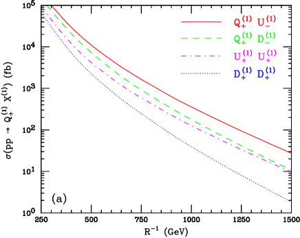
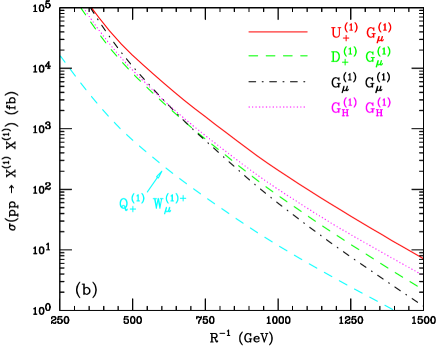
Figure 10: Tree-level production cross sections of (1,0) particles at the LHC: (a) quark pairs, and (b) final states involving bosons. The cross sections have been summed over the first two generations of KK quarks and antiquarks. The weak-doublet $Q^{{({\bf 1})}}_{+}$ includes both up- and down-type (1,0) quarks. The cross section for $U^{({\bf 1})}_{+}D^{({\bf 1})}_{+}$ production (not shown) turns out to be nearly equal to that for $U^{({\bf 1})}_{+}U^{({\bf 1})}_{+}$. Cross sections for the weak-singlet quarks (6D chirality $-$) are almost the same as those for weak-doublet quarks (6D chirality $+$) and are not plotted.

$Q_{+}^{({\bf 1})}Q_{+}^{({\bf 1})}$ production, which is responsible for most of the multi-lepton events (as shown later in Section 4.2), is dominated by (1,0) quarks of the first 2 generations (88% at $1/R=500$ GeV, increasing to 98% at $1/R=1$ TeV). The gluon-gluon initial state contributes only $\sim$10% (3%) of the total $Q_{+}^{({\bf 1})}Q_{+}^{({\bf 1})}$ cross section at $1/R=500$ GeV ($1$ TeV), since firstly the gluon flux in the proton at this mass scale is small, and secondly, there is a large number of subprocesses with $qq$ or $q\bar{q}$ initial states. $G_{H}^{({\bf 1})}$ production is different in that the dominant contribution to this process comes from the gluon initial state, with valence quarks making up the remainder.

The production cross sections of the $SU(2)_{W}$ doublet and singlet (1,0) quarks, $Q_{+}^{{({\bf 1})}}$ or $Q_{-}^{{({\bf 1})}}$, are almost equal, since they are produced in exactly the same way (see Figs. 3-6). The slightly higher mass of $Q_{+}^{{({\bf 1})}}$ lowers its production cross section, but this is a small effect. As expected from the structure of the parton distribution function, the $G_{\mu}^{{({\bf 1})}}$ associated production cross sections drop off faster than others.

$Q_{+}^{({\bf 1})}U_{-}^{({\bf 1})}$ pair production, the main source of events containing both photons and leptons, proceeds through $G_{\mu}^{({\bf 1})}$ and $G_{H}^{({\bf 1})}$ exchange in the $t$-channel, as in Fig. 3 with one of the $Q_{+}^{({\bf 1})}$ quarks replaced by $U_{-}^{({\bf 1})}$. Due to the partonic structure, the production with first-generation quarks in the initial state are dominant, accounting for $\sim 50\%$ of all $Q_{+}^{({\bf 1})}U_{-}^{({\bf 1})}$ pairs produced for $1/R=500$ GeV.

As mentioned earlier, $W_{\mu}^{{({\bf 1})}}$ associated production, although small compared to that for colored (1,0) particles, is not necessarily negligible because of its large branching fraction into leptons. We have included the cross section for the channel with the largest production rate, $W_{\mu}^{{({\bf 1})}+}Q_{+}^{{({\bf 1})}}$, in Fig. 10. The dominant contribution to this process is from production with first generation (1,0) quarks. $W_{\mu}^{{({\bf 1})}-}$ associated production is even smaller, by an extra factor of $\sim$3, due to the partonic structure of the proton.

4.2 Events with leptons and photons at the LHC

Having determined the production rates of (1,0) particles, we now turn to a discussion of their experimental signatures at the LHC. First we will consider the production of (1,0) particles which give $n\ell+m\gamma+\hbox to0.0pt{\,/\hss}E_{T}$ with $n\geq n_{min}$ and $0\leq m\leq 2$, where we do not count leptons from the decay of the standard model particles.

We calculate the inclusive cross sections for the channels $n\ell+m\gamma+\hbox to0.0pt{\,/\hss}E_{T}$ with $n\geq n_{min}$ and $0\leq m\leq 2$ in the following way. There are 11 (1,0) particles with different branching fractions to multiple leptons as discussed in Section 3. We label these particles by $A_{i}^{({\bf 1})}$, where $1\leq i\leq 11$ is the particle type:

$$A_{i}^{({\bf 1})}=\Big{(}W_{\mu}^{{({\bf 1})}},G_{\mu}^{{({\bf 1})}},G_{H}^{{({\bf 1})}},T_{+}^{{({\bf 1})}},B_{+}^{{({\bf 1})}},T_{-}^{{({\bf 1})}},U_{-}^{{({\bf 1})}},D_{-}^{{({\bf 1})}},Q_{+}^{{({\bf 1})}}\Big{)}\,.$$ (19)

Their branching fractions, Br$(i,a,a^{\prime})$, where $a$ is the number of leptons ($0\leq a\leq 4$) and $a^{\prime}$ is the number of photons ($0\leq a^{\prime}\leq 1$), are given in Section 3. $Q_{+}^{{({\bf 1})}}$ and $U^{({\bf 1})}_{-}$ include only the first two generations of weak doublets and up-type singlets. One should keep in mind that the 3rd generation KK quarks and KK quarks of the first two generations have different branching fractions to leptons so they need to be tackled separately. For simplicity we use the same symbol here for quarks and antiquarks. The cross section for $n\ell+m\gamma+\hbox to0.0pt{\,/\hss}E_{T}$ events with $n\geq n_{min}$ and $0\leq m\leq 2$ is

$$\sigma(pp\to n\ell+m\gamma+\hbox to0.0pt{\,/\hss}E_{T}~{},n\geq n_{min})=\sum_{i=1}^{11}\sum_{j\geq i}^{11}\sigma(pp\to A_{i}^{({\bf 1})}A_{j}^{({\bf 1})})B_{ij}\,,$$ (20)

where $B_{ij}$ is a sum over products of branching fractions of the particles $A_{i}^{({\bf 1})}$ and $A_{j}^{({\bf 1})}$

$$B_{ij}=\sum_{\underset{a+b\geq n_{min}}{a,b=0}}^{4}\sum_{\underset{a^{\prime}+b^{\prime}=m}{a^{\prime},b^{\prime}=0}}^{1}{\rm Br}(i,a,a^{\prime}){\rm Br}(j,b,b^{\prime})\,,$$ (21)

Note that the total numbers of photons ($m$) and leptons ($n$) from the decay of a pair of (1,0) particles are constrained by $0\leq n+2m\leq 8$. It is not possible to obtain $8\ell+2\gamma+\hbox to0.0pt{\,/\hss}E_{T}$ for instance, since the hypercharge gauge boson $B_{\mu}^{({\bf 1})}$ can decay into either a photon or a fermion pair, together with $B_{H}^{({\bf 1})}$, so a photon is only produced at the expense of two leptons. Most (1,0) particles have branching fractions that are independent of $1/R$. However, those for third generation quarks have variations due to threshold effects (see Fig. 2). We use values at large $1/R$, which slightly underestimates the total number of events as branching fractions are larger at small $1/R$. Since the contribution from the third generation is small, our approximation gives rise to negligible error.

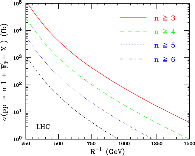
Figure 11: Sum over cross sections for (1,0) particle pair production at the LHC times the branching fractions of the cascade decays that give rise to $n\geq 3,4,5$ or 6 charged leptons ($\ell=e^{\pm}$ or $\mu^{\pm}$), as a function of the compactification scale.

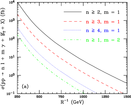
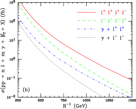
Figure 12: Cross sections for (a) $m\gamma+n\ell+\hbox to0.0pt{\,/\hss}E_{T}$ events with $n\geq n_{min}$ for $m=1,2$ and $1\leq n_{min}\leq 4$ and (b) Lepton + photon events with two or more same-sign leptons, at the LHC as a function of $1/R$.

Cross sections for multi-lepton events at the LHC are shown in Fig. 11 as a function of $1/R$. Out of the total number of events with 5 leptons or more at $1/R=500$ GeV, the majority arise from first- and second- generation weak doublet quarks, either in pairs or in association with other particles; $W_{\mu}^{({\bf 1})}$ pair production is responsible for around 10%, as is production including $SU(3)_{c}$ bosons, $G_{\mu,H}^{({\bf 1})}$. As parton distribution functions vary with the size of the extra dimensions, so will the individual contributions, although the sensitivity to the mass scale $1/R$ is small. The results shown in Fig. 11 include tree-level processes only. We estimate that next-to-leading order effects will increase the cross sections by $\sim$30-50%, especially due to initial state radiation. A complete analysis of this effect is warranted, but is beyond the scope of this paper.

Also interesting are combined photon and lepton events which result from 1-loop decays of the ${({\bf 1})}$ hypercharge gauge boson $B_{\mu}^{({\bf 1})}$ produced in the decay chain of $U_{-}^{({\bf 1})}$ quarks (see Fig. 12(a)). Down-type quarks have smaller hypercharge and so couple less strongly; while quark doublets couple more strongly to weak bosons, resulting in a negligible branching fraction into $B_{\mu}^{({\bf 1})}$. In Fig. 13 we show typical diagrams for $\ell^{+}\ell^{+}\ell^{+}\ell^{-}\ell^{-}$ and $\gamma\ell^{+}\ell^{-}$ signatures. The rate for events with unusual combinations of final states: two same-sign leptons and a photon, $\gamma\ell^{+}\ell^{+}$ ($\gamma\ell^{-}\ell^{-}$) for instance, or three same-sign and one opposite sign lepton, $\ell^{+}\ell^{+}\ell^{+}\ell^{-}$ ($\ell^{-}\ell^{-}\ell^{-}\ell^{+}$), are plotted in Fig. 12(b). The latter process consists of around 10% of the total rate for 4 lepton events, and the largest single contribution to it is the decay of $U_{+}^{({\bf 1})}$ ($D_{+}^{({\bf 1})}$) pairs. It arises only rarely in the standard model from $W^{+}W^{+}Z$ ($W^{-}W^{-}Z$) production.

  

Figure 13: Representative processes that lead to $5\ell+\hbox to0.0pt{\,/\hss}E_{T}$ and $\gamma\ell^{+}\ell^{-}+\hbox to0.0pt{\,/\hss}E_{T}$ events. Several other production mechanisms as well as cascade decays contribute to these and related signals.

We expect that the small standard model backgrounds for these processes can be eliminated by using a hard $\hbox to0.0pt{\,/\hss}E_{T}$ cut in conjunction with a jet $p_{T}$ cut since the jets originating from the decay of (1,0) colored particles should have a transverse momentum of the order of their mass differences ($\sim 100$ GeV). One might also naively worry about triggering issues due to the softness of leptons, since the cascade decays giving rise to them occur between particles that are relatively degenerate in mass. A preliminary analysis on a single leg of the decay chain keeping exact spin correlations suggests that more than 90 % of lepton pairs have enough $p_{T}$ to evade a 15 GeV cut, and that the leptons are far enough away in $\Delta R$ to be visible as individual tracks. Hence we do not anticipate any triggering problems, although a detailed analysis of these issues using a detector simulator might be beneficial.

4.3 Cross sections at the Tevatron

At the Tevatron, the production from a $q\bar{q}$ initial state, shown in Figs. 4, 7 and 9, dominates. We summarize our results for (1,0) production cross sections, as well as multi-lepton and lepton plus photon signatures in Fig. 14. The lower center-of-mass energy of this collider slightly increases $W_{\mu}^{({\bf 1})}$ production cross sections as compared with the LHC. This process now contributes 16% of the total number of events with 4 or more leptons for $1/R=300$ GeV.

We can use data gathered from Tevatron Run II to place rough constraints on the radius of the extra dimensions. One potential channel that has been searched for in the context of the minimal supersymmetric standard model is the trilepton signal [24, 25]. We apply the results of this analysis, which found no excess over standard model background, directly to our model. If we assume an efficiency of $\sim 5\%$ [24, 25], we see that $1/R$ must be larger than $\sim 270$ GeV, otherwise we might have expected to observe at least 3 events. Low statistics for this final state, both in expected and observed events, make the limit rather less reliable than desired.

A more precise, though less stringent, constraint can be obtained by using Run II lepton + photon data [26], which contains larger numbers of expected and observed events. The standard model prediction for the $\ell\gamma X$ channel for instance, is $150.6\pm 13$ with an observation of 163 events. Assuming that universal extra dimensions are responsible for the small excesses in this and the $\ell^{+}\ell^{-}\gamma X$ channels allows us to obtain a limit on $1/R$ of around 240 GeV at 95% C.L.

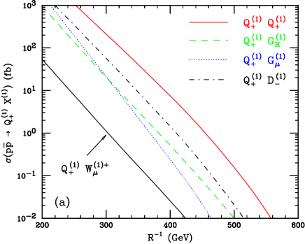
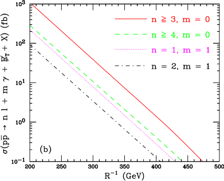
Figure 14: (a) Production cross sections at the Tevatron and (b) Cross sections for multilepton + photon events, as a function of $1/R$.

5 Conclusions

Despite the successful predictions of the 6DSM, the hadron collider phenomenology of (1,0) KK modes has not been previously studied due to the large number of mechanisms that contribute to production cross sections. Our inclusion in CalcHEP of the interactions between (1,0) particles and standard model ones has allowed us to compute the cross sections for (1,0) pair production at the LHC and the Tevatron. The large cross sections (of almost $10^{4}$ fb at the LHC, for masses around 500 GeV) shows that cascade decays with small branching fractions may be observed, leading to a variety of discovery channels. These are particularly interesting because of the presence in the 4D effective theory of a spinless adjoint particle for each standard model gauge group. One-loop corrections to the level-1 masses tend to make these spinless adjoints lighter than matter fields [14] (the same result [27] applies to other models [28]), forcing them to undergo tree-level 3-body decays and emitting two standard model fermions each time. This results in significant numbers of events with five or more leptons.

Multi-lepton events are not unique to the 6DSM, although the rates at which they occur in other theories are typically smaller. In its 5D counterpart for example, it is necessary to produce level-2 KK particles to give rise to long enough cascades; the rate for such processes is suppressed because the particles produced are heavier ($m\sim 2/R$) [4]. Another theory leading to multi-lepton signatures involves a warped extra dimension with custodial symmetry [29], but leptons in that case come from decays of $W$ and $Z$, whose branching fractions are small. In supersymmetric models, cascade decays of squarks such as $\tilde{q}^{\prime}_{L}\to\tilde{\chi}_{2}^{\pm}q\to W^{\pm}\tilde{\chi}_{2}^{0}q(\tilde{\chi}_{1}^{\pm}Zq)$ can also give multi-lepton signatures at the cost of small production cross sections due to spin-statistics as well as a small branching fraction for $\tilde{q}^{\prime}_{L}\to\tilde{\chi}_{2}^{\pm}q$.

Nevertheless, it should be rather straightforward to differentiate among these models if a sufficiently large number of multi-lepton events will be observed at the LHC. The 6DSM has specific preditions for many observables. In this paper we analyzed the rates for events with 3, 4, 5 and 6 leptons, as well as the relative rates for events with three leptons of one charge and one lepton of opposite charge. Other observables, such as the relative rates for events with different numbers of electrons and muons, may be analyzed using the branching fractions for complete cascade decays (see the tables in Section 3). Another peculiarity of the 6DSM cascade decays is that they lead with reasonably large branching fractions to events with photons. This is a consequence of the 2-body decay at one loop of the hypercharge (1,0) vector boson, which competes successfully with its tree-level 3-body decays. Events with leptons, photons and missing energy are also predicted in certain supersymmetric extensions of the standard model, but again, there are several different channels, and we expect that if such events will be seen in large numbers, it will be possible to differentiate between models.

One may wonder how robust our predictions are against variations in the mass spectrum, which may get contributions from operators localized at the fixed points of the chiral square, as well as from higher-order QCD effects. In the case of a single universal extra dimension, deviations from the one-loop corrected mass spectrum lead to a variety of phenomenological implications [30]. Within the 6DSM, we expect that the rates for multi-lepton events remain relatively large when the (1,0) mass spectrum is perturbed. This is due to the large number of particles involved in a typical decay chain, with a standard model quark or lepton being emitted at each stage. The total rates computed here are sums over many such cascade decays of several (1,0) particles. However, the events with photons depend entirely on the branching fractions of a single particle, the hypercharge vector boson, and thus are less generic for different mass spectra.

A more general approach would be to lift the constraints on the mass spectrum. If excess events with leptons, missing energy and possibly photons will be observed in certain channels at the LHC, then the (1,0) masses would be determined by comparing a large set of observed rates with the 6DSM predictions. One should also keep in mind that the predictions of the 6DSM are not limited to collider signals. For example, an interesting feature is that the LKP has spin 0, with various implications for dark matter [31].

Acknowledgments:  We would like to thank Hsin-Chia Cheng, Konstantin Matchev and Eduardo Ponton for helpful conversations. Fermilab is operated by Fermi Research Alliance, LLC under Contract No. DE-AC02-07CH11359 with the United States Department of Energy.

Appendix A:  Feynman rules for (1,0) modes

In this section we show Feynman rules that are relevant for QCD production of (1,0) particles at hadron colliders. Corresponding vertices involving electroweak gauge bosons can be easily inferred from those given below. The vector-like nature of KK fermions allows for the usual QCD coupling to standard model gluons seen in the $G_{\mu}Q^{{({\bf 1})}}\overline{Q}{{}^{({\bf 1})}}$ vertex below.

The interaction of a level-1 quark and a level-1 gluon is chiral and so its vertex contains projection operators, although the chirality of the incoming fermion is conserved.

However, the interaction of a spinless adjoint $G_{H}^{(1,0)a}$ with fermions changes the chirality of the incoming fermion since $G_{H}^{(1,0)a}$ is a scalar. Note that the Feynman rules for standard-model gluons are fixed by gauge invariance. The 3 and 4-point interactions involving only (1,0) vector bosons and zero-mode gluons are identical to those in the standard model.

Appendix B:  One-loop 2-body decays of (1,0) bosons

We compute here the amplitude for the process $B_{\nu}^{{({\bf 1})}}\rightarrow B_{H}^{{({\bf 1})}}\gamma$, which proceeds through one-loop diagrams with KK fermions running in the loop. The couplings of the $B_{\nu}^{{({\bf 1})}}$ and $B_{H}^{{({\bf 1})}}$ bosons to the KK modes of a 6D chiral fermion $F_{+}$ are given by

$$\mathcal{L}\supset\frac{1}{4}g^{\prime}Y_{F_{+}}\overline{F}_{+}^{(j,k)} \left[B_{\nu}^{{({\bf 1})}}\gamma^{\nu}\left(P_{L}\,d_{00}^{j,k;j^{\prime}\!,k^{\prime}}-P_{R}\,d_{10}^{j,k;j^{\prime}\!,k^{\prime}}r_{jk}^{*}r_{j^{\prime},k^{\prime}}\right)\right.$$ (B.1)

$$\left.\ -\,iB_{H}^{{({\bf 1})}}\left(P_{R}\,d_{01}^{j,k;j^{\prime}\!,k^{\prime}}r_{j^{\prime},k^{\prime}}-P_{L}\,d_{03}^{j^{\prime}\!,k^{\prime}\!;j,k}r_{jk}^{*}\right)\right]F_{+}^{j^{\prime},k^{\prime}}~{}.$$

Here we have defined

$$d_{nn^{\prime}}^{j,k;j^{\prime}\!,k^{\prime}} = (-1)^{n}\delta_{k^{\prime}\!,k}\left(\delta_{j^{\prime}\!,j-1}+(-1)^{n^{\prime}}\delta_{j^{\prime}\!,j+1}\right)+(-1)^{n}\delta_{j^{\prime}\!,j}\left(\delta_{k^{\prime}\!,k+1}+(-1)^{n^{\prime}}\delta_{k^{\prime}\!,k-1}\right)$$ (B.2)

$$+\,i^{n^{\prime}-n}\delta_{j,1}\delta_{k^{\prime}\!,0}\delta_{j^{\prime}\!,k}+i^{n+2n^{\prime}}\delta_{j^{\prime}\!,1}\delta_{k,0}\delta_{k^{\prime}\!,j}~{},$$

where $r_{j,k}$ are complex phases,

$$r_{j,k}=\frac{j+ik}{\sqrt{j^{2}+k^{2}}}$$ (B.3)

and $Y_{F}$ is the hypercharge of the fermion, normalized to $-1$ for lepton doublets. In the case of fermions with 6D chirality $-$, which contain right-handed zero modes, the same formulas apply with the $P_{L}$ and $P_{R}$ chirality projection operators interchanged.

Figure 15: Dimension-5 operator induced by fermion loops.

Dimension-5 operators coupling a (1,0) vector boson to a (1,0) spinless adjoint and a standard-model gauge boson are induced at one loop by the diagram in Figure 15, with fermion KK modes running in the loop. The contribution of a fermion $F_{+}$ to the amplitude for $B_{\nu}^{{({\bf 1})}}\rightarrow B_{H}^{{({\bf 1})}}\gamma_{\mu}$ is given by

$${\cal M}\left(B_{\nu}^{({\bf 1})}\rightarrow B_{H}^{({\bf 1})}\gamma_{\mu}\right)_{F_{+}}=-\frac{1}{4}\left(g^{\prime}\frac{Y_{F_{+}}}{2}\right)^{\!2}e\,Q_{F_{+}}\,\varepsilon_{\mu}^{*}(p-p^{\prime})\,\varepsilon_{\nu}(p)\,I_{F_{+}}^{\mu\nu(j,k;j^{\prime}\!,k^{\prime})}~{},$$ (B.4)

where

$$I_{F_{+}}^{\mu\nu(j,k;j^{\prime}\!,k^{\prime})}=\int\!\!\frac{d^{4}l}{(2\pi)^{4}}{\rm Tr}\frac{m_{F}^{j,k;j^{\prime}\!,k^{\prime}}\left[l\!\!/\gamma^{\mu}+\gamma^{\mu}(l\!\!/+p\!\!\!/-p^{\prime}\!\!\!\!/)\right](l\!\!/+p\!\!\!/)-m_{F}^{j^{\prime}\!,k^{\prime}\!;j,k}l\!\!/\gamma^{\mu}(l\!\!/+p\!\!\!/-p^{\prime}\!\!\!\!/)}{\left(l^{2}-M^{2}_{F^{(j,k)}}\right)\left[(l+p-p^{\prime})^{2}-M^{2}_{F^{(j,k)}}\right]\left[(l+p)^{2}-M^{2}_{F^{(j^{\prime},k^{\prime})}}\right]}\gamma^{\nu}\gamma_{5}$$ (B.5)

and

$$m^{j,k;j^{\prime}\!,k^{\prime}}_{F}=M_{F^{(j,k)}}\,{\rm Re}\left[r_{jk}\left(d_{00}^{j,k;j^{\prime}\!,k^{\prime}}d_{01}^{j^{\prime}\!,k^{\prime}\!;j,k}-d_{10}^{j^{\prime}\!,k^{\prime}\!;j,k}d_{01}^{j,k;j^{\prime}\!,k^{\prime}}\right)\right]~{}.$$ (B.6)

After integrating over the loop momentum $l$, and summing over fermions, we find the amplitude

$${\cal M}\left(B_{\nu}^{({\bf 1})}\rightarrow B_{H}^{({\bf 1})}\gamma_{\mu}\right)=-\frac{g^{\prime 2}e}{8\pi^{2}}\epsilon^{\mu\nu\alpha\beta}\frac{\varepsilon_{\mu}^{*}(p-p^{\prime})\varepsilon_{\nu}(p)p_{\alpha}p^{\prime}_{\beta}}{M_{B_{\nu}^{({\bf 1})}}^{2}-M_{B_{H}^{({\bf 1})}}^{2}}\sum_{F}\sigma_{F}\,\left(\frac{Y_{F}}{2}\right)^{2}\,Q_{F}\,{\cal E}_{F}~{},$$ (B.7)

where $\sigma_{F}=\pm 1$ when $F$ has 6D chirality $\pm$, and

$${\cal E}_{F}=\sum_{j,k;j^{\prime}\!,k^{\prime}}m_{F}^{j,k;j^{\prime}\!,k^{\prime}}J_{F}^{j,k;j^{\prime}\!,k^{\prime}}~{},$$ (B.8)

with $J_{F}$ given by an integral over a Feynman parameter:

$$J_{F}^{j,k;j^{\prime}\!,k^{\prime}}=\int_{0}^{1}\frac{dx}{x}\ln\left(1+\frac{x(1-x)\left(M_{B_{\nu}^{({\bf 1})}}^{2}-M_{B_{H}^{({\bf 1})}}^{2}\right)}{(1-x)M_{F^{(j,k)}}^{2}+xM_{F^{(j^{\prime}\!,k^{\prime})}}^{2}-x(1-x)M_{B_{\nu}^{({\bf 1})}}^{2}}\right)~{}.$$ (B.9)

The $m^{j,k;j^{\prime}\!,k^{\prime}}$ quantities vanish unless the set of KK numbers $(j,k;j^{\prime}\!,k^{\prime})$ is given by (1,0;1,1), (1,1;1,0) or (1,0; 0,0). This is a consequence of the vectorlike nature of the fermion higher KK modes. Therefore,

$${\cal E}_{F}=M_{F^{(1,0)}}\left(2J_{F}^{1,0;0,0}+J_{F}^{1,0;1,1}\right)+\sqrt{2}M_{F^{(1,1)}}J_{F}^{1,1;1,0}~{}.$$ (B.10)

Note that ${\cal E}_{F}$ depends only on the (1,0) masses and on the masses of the (0,0) and (1,1) fermions. The mass corrections for (1,1) fermions, $\big{\{}Q^{3}_{+},T_{-},Q^{1,2}_{+},U^{1,2}_{-},D^{1,2,3}_{-},L_{+}$ and $E_{-}\big{\}}$, are given by $\sqrt{2}/R$ multiplied by the coefficients $\left\{1.33,1.31,1.31,1.27,1.26,1.05,1.02\right\}$ respectively [5], ignoring electroweak symmetry breaking effects. Note also that in the limit that all the fermions at each KK level are degenerate, ${\cal E}_{F}$ becomes independent of $F$ and so can be taken out of the sum in Eq. (B.7), which then vanishes identically by anomaly cancellation. This completes the computation of the amplitude for $B_{\nu}^{{({\bf 1})}}\rightarrow B_{H}^{{({\bf 1})}}\gamma$, which determines the coefficient of the dimension-5 operator shown in Eq. (11), and the decay width of $B_{\nu}^{{({\bf 1})}}$ shown in Eq. (5).

Appendix C:  Tree-level 3-body decays of (1,0) bosons

Figure 16: The diagrams for 3-body decay of (1,0) particles. $A_{2}$ and $A_{1}$ are heavy bosons of spin 0 or 1, $F$ is a heavier fermion, and $f$ is a much lighter fermion.

In this Appendix we compute the width for 3-body decays of (1,0) bosons. Let us consider a generic 3-body decay of a boson $A_{2}$ of mass $M_{2}$ into a boson $A_{1}$ of mass $M_{1}$ and a fermion-antifermion pair $f\bar{f}$, via an off-shell fermion $F$, of mass $M_{F}>M_{2}>M_{1}$. There are two tree-level diagrams contributing to the process $A_{2}\to(F^{\ast}f)\to A_{1}f\bar{f}$, as shown in Fig. 16. For simplicity, we assume that the final-state fermions are massless. The decay width is given by

$$\Gamma(A_{2}\to A_{1}f\bar{f})=\frac{1}{64\pi^{3}M_{2}}\int_{0}^{\mu_{\circ}}dE_{f}\int_{\mu_{\circ}-E_{f}}^{E_{\bar{f}}^{\rm max}}dE_{\bar{f}}\,\,\overline{\left|\cal{M}\right|^{2}}~{},$$ (C.1)

where $\cal{M}$ is the matrix element, $E_{f}$ and $E_{\bar{f}}$ are the energies of the final-state fermions in the rest frame of $A_{2}$, and we defined

$$\mu_{\circ}\equiv\frac{M_{2}^{2}-M_{1}^{2}}{2M_{2}}\,.$$ (C.2)

For a fixed $E_{f}$, the maximum value of $E_{\bar{f}}$ is

$$E_{\bar{f}}^{\rm max} = \frac{\mu_{\circ}-E_{f}}{1-2E_{f}/M_{2}}\,.$$ (C.3)

Let us first consider the case where both $A_{1}$ and $A_{2}$ have spin 0 (we label them by $A_{1H}$ and $A_{2H}$ in that case) and have pseudo-scalars couplings to the fermions:

$$\left(g_{1}A_{1H}+g_{2}A_{2H}\right)i\overline{F}_{L}f_{R}+{\rm H.c.}~{},$$ (C.4)

where $g_{1,2}$ are real dimensionless couplings. The matrix element squared, summed over the spins of $f$ and $\bar{f}$, is given by

$$\overline{\left|{\cal M}\right|^{2}}\left(A_{2H}\to f_{R}\bar{f}_{R}A_{1H}\right)=2\left(g_{1}g_{2}\right)^{2}\Big{[}2(P_{f}\cdot P_{1})(P_{f}\cdot P_{1})-M_{2}^{2}(P_{f}\cdot P_{\bar{f}})\Big{]}\,\Delta^{2}~{},$$ (C.5)

where $P_{1}$, $P_{f}$ and $P_{\bar{f}}$ are the 4-momenta of $A_{1H}$, $f$ and $\bar{f}$, respectively. The quantity

$$\Delta=\frac{1}{(P_{1}+P_{f})^{2}-M_{F}^{2}}-\frac{1}{(P_{1}+P_{\bar{f}})^{2}-M_{F}^{2}}\,,$$ (C.6)

accounts for the propagators of the off-shell fermion in the two diagrams of Fig. 16. The two diagrams have opposite sign, resulting in the sign between the two terms in $\Delta$, because of the different momentum flow through the intermediate fermion line. In the center-of-mass frame, the width becomes

$$\Gamma(A_{2H}\to A_{1H}f_{R}\bar{f}_{R})=\frac{\left(g_{1}g_{2}\right)^{2}}{128\pi^{3}}M_{2}\,{\cal I}_{+}(M_{2},M_{1},M_{F})$$ (C.7)

where we defined

$${\cal I}_{\pm}(M_{2},M_{1},M_{F})=\int_{0}^{\mu_{\circ}}dE_{f}\int_{\mu_{\circ}-E_{f}}^{E_{\bar{f}}^{\rm max}}\!dE_{\bar{f}}\;\frac{2E_{f}E_{\bar{f}}\pm M_{2}\left(\mu_{\circ}-E_{f}-E_{\bar{f}}\right)}{M_{2}^{2}(\mu_{\star}+E_{f})^{2}(\mu_{\star}+E_{\bar{f}})^{2}}\left(E_{f}-E_{\bar{f}}\right)^{2}~{}.$$ (C.8)

The function ${\cal I}_{-}$ is introduced for later convenience, $\mu_{\circ}$ and $E_{\bar{f}}^{\rm max}$ are given in Eqs. (C.2) and (C.3), respectively, and

$$\mu_{\star}\equiv\frac{M_{F}^{2}-M_{2}^{2}}{2M_{2}}~{}~{}.$$ (C.9)

Let us now study the case where $A_{2}$ has spin 1 (we label it by $A_{2\mu}$ in that case) and couples to one chirality of the fermions:

$$g_{2}A_{2\mu}\overline{F}_{R}\gamma^{\mu}f_{R}+{\rm H.c.}~{}.$$ (C.10)

The matrix element squared, averaged over the polarizations of $A_{2\mu}$ and summed over the spins of $f$ and $\bar{f}$, is given by

$$\overline{\left|{\cal M}\right|^{2}}\left(A_{2\mu}\to f_{R}\bar{f}_{R}A_{1H}\right)=\frac{2}{3}\left(g_{1}g_{2}\right)^{2}\left(\frac{M_{F}}{M_{2}}\right)^{\!2}\Big{[}2(P_{f}\cdot P_{2})(P_{\bar{f}}\cdot P_{2})+M_{2}^{2}P_{f}\cdot P_{\bar{f}}\Big{]}\Delta^{2}~{},$$ (C.11)

where $P_{2}$ is the 4-momentum of $A_{2H}$. Again, the two diagrams have opposite signs, resulting in the form of $\Delta$ given in Eq. (C.6). However, the sign difference in this case is due to the pseudo-scalar coupling. The width in the center-of-mass frame is given by

$$\Gamma(A_{2\mu}\to A_{1H}f_{R}\bar{f}_{R})=\frac{\left(g_{1}g_{2}\right)^{2}}{384\pi^{3}}\frac{M_{F}^{2}}{M_{2}}\,{\cal I}_{-}(M_{2},M_{1},M_{F})~{},$$ (C.12)

where ${\cal I}_{-}$ is the phase-space integral shown in Eq. (C.8).

The only other case relevant for the decays of the (1,0) particles discussed in Section 3 is that where $A_{2}$ has spin 0 and pseudo-scalar couplings [see Eq. (C.4)], while $A_{1}$ has spin 1 and a coupling

$$g_{1}A_{1\mu}\overline{F}_{R}\gamma^{\mu}f_{R}+{\rm H.c.}~{}.$$ (C.13)

The matrix element squared, summed over the polarizations of $A_{1\mu}$ and the spins of $f$ and $\bar{f}$, is given in this case by

$$\overline{\left|{\cal M}\right|^{2}}\left(A_{2H}\to f_{R}\bar{f}_{R}A_{1\mu}\right)=2\left(g_{1}g_{2}\right)^{2}\left(\frac{M_{F}}{M_{1}}\right)^{\!2}\Big{[}2(P_{f}\cdot P_{1})(P_{\bar{f}}\cdot P_{1})+M_{2}^{2}P_{f}\cdot P_{\bar{f}}\Big{]}\Delta^{2}~{},$$ (C.14)

where $\Delta$ is defined in Eq. (C.6). The width in the center-of-mass frame is given by

$$\Gamma(A_{2H}\to A_{1\mu}{\cal I}_{R}\bar{f}_{R})=\frac{\left(g_{1}g_{2}\right)^{2}}{128\pi^{3}}M_{2}\frac{M_{F}^{2}}{M_{1}^{2}}\,\left[\left(1-\frac{2\mu_{\circ}}{M_{2}}\right){\cal I}_{-}(M_{2},M_{1},M_{F})+\frac{2\mu_{\circ}}{M_{2}}{\cal I}_{+}(M_{2},M_{1},M_{F})\right]~{}.$$ (C.15)

If the heavy particles are approximately degenerate, which is the case for the (1,0) particles studied in this paper, then $\mu_{\circ}\ll M_{2}$ and $\mu_{\star}\ll M_{2}$ (which implies $\mu_{\circ}\approx M_{2}-M_{1}$ and $\mu_{\star}\approx M_{F}-M_{2}$), and the double integrals of Eq. (C.8) may be performed analytically:

$${\cal I}_{+}(M_{2},M_{1},M_{F}) = \frac{-8}{M_{2}^{3}}\left[\rule{0.0pt}{14.22636pt}\mu_{\star}\frac{\mu_{\circ}+\mu_{\star}}{\mu_{\circ}+2\mu_{\star}}\left(\mu_{\circ}^{2}+5\mu_{\circ}\mu_{\star}+5\mu_{\star}^{2}\right)\ln\left(1+\frac{\mu_{\circ}}{\mu_{\star}}\right)\right.$$ (C.16)

$$\;\;\;-\left.\frac{\mu_{\circ}}{12}\left(\mu_{\circ}^{2}+30\mu_{\circ}\mu_{\star}+30\mu_{\star}^{2}\right)\rule{0.0pt}{14.22636pt}\right]\left[1+O\left(\frac{\mu_{\circ}}{M_{2}},\frac{\mu_{\star}}{M_{2}}\right)\right]~{}.$$

A simple relation between the ${\cal I}_{\pm}$ functions holds at leading order in $1/M_{2}$:

$${\cal I}_{-}=3{\cal I}_{+}\left[1+O\left(\frac{\mu_{\circ}}{M_{2}},\frac{\mu_{\star}}{M_{2}}\right)\right]~{}.$$ (C.17)

It is also useful to note that for $\mu_{\circ}\ll M_{2}$ and $\mu_{\circ}\ll\mu_{\star}$,

$${\cal I}_{+}(M_{2},M_{1},M_{F}) = \frac{\mu_{\circ}^{7}}{105\,M_{2}^{3}\mu_{\star}^{4}}\left[1-2\frac{\mu_{\circ}}{\mu_{\star}}+\frac{\mu_{\circ}}{M_{2}}+O\left(\frac{\mu_{\circ}^{2}}{\mu_{\star}^{2}},\,\frac{\mu_{\circ}^{2}}{M_{2}^{2}}\right)\right]~{},$$

$${\cal I}_{-}(M_{2},M_{1},M_{F}) = \frac{\mu_{\circ}^{7}}{35\,M_{2}^{3}\mu_{\star}^{4}}\left[1-2\frac{\mu_{\circ}}{\mu_{\star}}+\frac{5\mu_{\circ}}{3M_{2}}+O\left(\frac{\mu_{\circ}^{2}}{\mu_{\star}^{2}},\,\frac{\mu_{\circ}^{2}}{M_{2}^{2}}\right)\right]~{}.$$ (C.18)

This very strong dependence on $\mu_{\circ}\approx M_{2}-M_{1}$ is somewhat surprising. The phase-space integrals of Eq. (C.8) give three powers of $\mu_{\circ}$, and the matrix element squared appears at first sight to give only one more power of $\mu_{\circ}$. However, the relative sign of the two diagrams forces a cancellation of the leading term within $\Delta$ [see Eq. (C.6)], so that $\Delta^{2}$ gives the $\left(E_{f}-E_{\bar{f}}\right)^{2}$ factor in Eq. (C.8), which accounts for two more powers of $\mu_{\circ}$. Furthermore, the integration over $E_{\bar{f}}$ cancels the leading term in the $\mu_{\circ}$ expansion of the numerator of ${\cal I}_{\pm}$. The resulting dependence on the 7th power of $\mu_{\circ}$ implies that the decay width is extremely suppressed, if $A_{2}$ and $A_{1}$ are more degenerate than the $F-A_{2}$ pair.

The decay widths given in Eqs. (C.7) and (C.15) are used in Section 3 for computing the branching fractions of the spinless adjoints, while the decay width of Eqs. (C.12) determines the branching fractions of the (1,0) hypercharge vector boson.

References

• [1] T. Appelquist, H. C. Cheng and B. A. Dobrescu, “Bounds on universal extra dimensions,” Phys. Rev.  D 64, 035002 (2001) [arXiv:hep-ph/0012100].
• [2] H. C. Cheng and I. Low, “TeV symmetry and the little hierarchy problem,” JHEP 0309, 051 (2003) [arXiv:hep-ph/0308199].
• [3] H. C. Cheng, K. T. Matchev and M. Schmaltz, “Bosonic supersymmetry? Getting fooled at the LHC,” Phys. Rev.  D 66, 056006 (2002) [arXiv:hep-ph/0205314].
• [4] A. Datta, K. Kong and K. T. Matchev, “Discrimination of supersymmetry and universal extra dimensions at hadron colliders,” Phys. Rev. D 72, 096006 (2005) [Erratum-ibid. D 72, 119901 (2005)] [arXiv:hep-ph/0509246].
• [5] G. Burdman, B. A. Dobrescu and E. Ponton, “Resonances from two universal extra dimensions,” Phys. Rev.  D 74, 075008 (2006) [arXiv:hep-ph/0601186].
• [6] G. Burdman, B. A. Dobrescu and E. Ponton, “Six-dimensional gauge theory on the chiral square,” JHEP 0602, 033 (2006) [arXiv:hep-ph/0506334].
• [7] B. A. Dobrescu and E. Pontón, “Chiral compactification on a square,” JHEP 0403, 071 (2004) [arXiv:hep-th/0401032].
• [8] M. Hashimoto and D. K. Hong, “Topcolor breaking through boundary conditions,” Phys. Rev.  D 71, 056004 (2005) [arXiv:hep-ph/0409223].
• [9] B. A. Dobrescu and E. Poppitz, “Number of fermion generations derived from anomaly cancellation,” Phys. Rev. Lett.  87, 031801 (2001) [arXiv:hep-ph/0102010].
• [10] T. Appelquist, B. A. Dobrescu, E. Ponton and H. U. Yee, “Proton stability in six dimensions,” Phys. Rev. Lett.  87, 181802 (2001) [arXiv:hep-ph/0107056].
• [11] For reviews, see:
D. Hooper and S. Profumo, “Dark matter and collider phenomenology of universal extra dimensions,” arXiv:hep-ph/0701197.
G. D. Kribs, “Phenomenology of extra dimensions,” arXiv:hep-ph/0605325.
• [12] H. C. Cheng, K. T. Matchev and M. Schmaltz, “Radiative corrections to Kaluza-Klein masses,” Phys. Rev.  D 66, 036005 (2002) [arXiv:hep-ph/0204342].
• [13] G. Servant and T. M. P. Tait, “Is the lightest Kaluza-Klein particle a viable dark matter candidate?,” Nucl. Phys.  B 650, 391 (2003) [arXiv:hep-ph/0206071].
H. C. Cheng, J. L. Feng and K. T. Matchev, “Kaluza-Klein dark matter,” Phys. Rev. Lett.  89, 211301 (2002) [arXiv:hep-ph/0207125].
• [14] E. Ponton and L. Wang, “Radiative effects on the chiral square,” JHEP 0611, 018 (2006) [arXiv:hep-ph/0512304].
• [15] Z. Chacko, H. S. Goh and R. Harnik, “The twin Higgs: Natural electroweak breaking from mirror symmetry,” Phys. Rev. Lett.  96, 231802 (2006) [arXiv:hep-ph/0506256].
• [16] G. Burdman and A. G. Dias, “The little hierarchy in universal extra dimensions,” JHEP 0701, 041 (2007) [arXiv:hep-ph/0609181].
See also G. Burdman, “Two universal extra dimensions,” arXiv:hep-ph/0611064.
• [17] C. Macesanu, C. D. McMullen and S. Nandi, “Collider implications of universal extra dimensions,” Phys. Rev.  D 66, 015009 (2002) [arXiv:hep-ph/0201300].
J. M. Smillie and B. R. Webber, “Distinguishing spins in supersymmetric and universal extra dimension models at the Large Hadron Collider,” JHEP 0510, 069 (2005) [arXiv:hep-ph/0507170].
T. G. Rizzo, “Probes of universal extra dimensions at colliders,” Phys. Rev.  D 64, 095010 (2001) [arXiv:hep-ph/0106336].
C. Macesanu, “The phenomenology of universal extra dimensions at hadron colliders,” Int. J. Mod. Phys.  A 21, 2259 (2006) [arXiv:hep-ph/0510418].
• [18] A. Pukhov et al., “CompHEP: A package for evaluation of Feynman diagrams and integration over multi-particle phase space. User’s manual for version 33,” arXiv:hep-ph/9908288.
• [19] A. Pukhov, “CalcHEP 3.2: MSSM, structure functions, event generation, batchs, and generation of matrix elements for other packages,” arXiv:hep-ph/0412191.
• [20] Our CalcHEP files are available at http//theory.fnal.gov/people/kckong/6D.
• [21] T. Stelzer and W. F. Long, “Automatic generation of tree level helicity amplitudes,” Comput. Phys. Commun.  81, 357 (1994) [arXiv:hep-ph/9401258].
• [22] F. Maltoni and T. Stelzer, “MadEvent: Automatic event generation with MadGraph,” JHEP 0302, 027 (2003) [arXiv:hep-ph/0208156].
• [23] J. Pumplin, D. R. Stump, J. Huston, H. L. Lai, P. Nadolsky and W. K. Tung, “New generation of parton distributions with uncertainties from global QCD analysis,” JHEP 0207, 012 (2002) [arXiv:hep-ph/0201195].
• [24] CDF Collaboration, “Combined limit for the trileptons analyses”, CDF Note 8653.
• [25] D0 Collaboration, “Search for the Associated Production of Chargino and Neutralino in Final States with Two Electrons and an Additional Lepton”, D0 Note 5127-Conf.
• [26] A. Abulencia, “Search for new physics in lepton + photon + X events with 929-pb-1 of $p\bar{p}$ collisions at $\sqrt{s}=1.96$ TeV”,  arXiv:hep-ex/0702029.
• [27] A. T. Azatov, “Radiative corrections to the lightest KK states in the $T2/(Z_{2}\times Z_{2}^{\prime})$ orbifold,” arXiv:hep-ph/0703157.
• [28] R. N. Mohapatra and A. Perez-Lorenzana, “Neutrino mass, proton decay and dark matter in TeV scale universal extra dimension models,” Phys. Rev.  D 67, 075015 (2003) [arXiv:hep-ph/0212254].
K. Hsieh, R. N. Mohapatra and S. Nasri, “Dark matter in universal extra dimension models: Kaluza-Klein photon and right-handed neutrino admixture,” Phys. Rev.  D 74, 066004 (2006) [arXiv:hep-ph/0604154].
• [29] C. Dennis, M. K. Unel, G. Servant and J. Tseng, “Multi-W events at LHC from a warped extra dimension with custodial symmetry,” arXiv:hep-ph/0701158.
• [30] J. A. R. Cembranos, J. L. Feng and L. E. Strigari, “Exotic collider signals from the complete phase diagram of minimal universal extra dimensions,” Phys. Rev.  D 75, 036004 (2007) [arXiv:hep-ph/0612157].
• [31] B.A. Dobrescu, D. Hooper, K. Kong, R. Mahbubani, work in progress.