Study of $X(1812)$ as a $(K^{*}\bar{K}^{*})$ Molecular State

Abstract

We investigate the decay and the production mechanism of the resonance $X(1812)$ recently observed in the $J/\psi\to\gamma X(1812),~{}X(1812)\to\omega\phi$ at BESII. The decay widths of $X(1812)\to\eta\eta^{\prime}$,$~{}\eta\eta$,$~{}\omega\phi$,$~{}K^{+}K^{-}$,$~{}\rho^{+}\rho^{-}$, $~{}\omega\omega$,$~{}K^{*+}K^{*-}$ and $\pi^{+}\pi^{-}$ are evaluated based on the scenario of the $X(1812)$ as a candidate of $(K^{*}\bar{K}^{*})$ molecule. It turns out that the quark exchange mechanism plays an important role in the understanding of the large decay width for the $X(1812)\to\omega\phi$. It is also found that the decay widths for $X(1812)\to\eta\eta^{\prime}$ and $\eta\eta$ are enhanced by the quark exchange mechanism. These channels are suggested to be the tools to test the molecular scenario in experiment. The branching fraction of $Br(X\to\omega\phi)$ is evaluated to be about $4.60\%$. Searches for additional evidence about the $X(1812)$ in $J/\psi$ radiative decays are reviewed. In the molecular scenario, the $X(1812)$ production rate is also evaluated to be $\Gamma(J/\psi\to\gamma X)/\Gamma(J/\psi\to\gamma K^{*+}K^{*-})=2.13^{+7.41}_{-1.85}$, which is close to the measured value $2.83\pm 0.92$.

PACS:13.20.Gd, 12.39.-x, 13.30.Eg.
Key words: $J/\psi$, Quark model, Molecular state, exotic state.

1 Introduction

The observation of a near-threshold enhancement in $J/\psi\to\gamma X,~{}X\to\omega\phi$ at BESII [1] immediately provokes discussion about its nature. This enhancement is reported to favor $J^{PC}=0^{++}$ in a partial wave analysis with a mass and width of $M=1812^{+19}_{-26}(\textrm{stat})\pm 18(\textrm{syst})$ and $\Gamma=105\pm 20(\textrm{stat})\pm 28(\textrm{syst})$ MeV, respectively, and a production branching ratio, $B(J/\psi\to\gamma X)\cdot B(X\to\omega\phi)=[2.61\pm 0.27(\textrm{stat})\pm 0.65(\textrm{syst})]\times 10^{-4}$. This resonant state is named as $X(1812)$ in the following part.

Emergence of the $X(1812)$ adds a new puzzle to the scalar sector of mesons. The most interesting feature about $X(1812)$ is that it seems to have a strange production and decay mechanism observed in the $J/\psi\to\gamma\omega\phi$. If the valence quarks of $\omega$ and $\phi$ are assigned as $(u\bar{u}+d\bar{d})/\sqrt{2}$ and $s\bar{s}$, one expects that this double OZI suppressed process should have a smaller branching fraction, at least less than the OZI allowed processes, e.g. $J/\psi\to\gamma\phi\phi$ or $\gamma\omega\omega$. It seems that the $X(1812)$ has a large contribution to the $J/\psi\to\gamma\omega\phi$ decay. Moreover, if the scalar of $X(1812)$ is assigned as the $q\bar{q}$ ordinary meson, it weakly couples to the decay mode of $\omega\phi$ and has a small phase space to decay into $\omega\phi$ near the threshold. However, the observed branching fraction is at the order of $10^{-4}$. So it is difficult to fit the $X(1812)$ into the spectrum of ordinary $q\bar{q}$ mesons. Many efforts have been made to interpret the $X(1812)$ as an exotic state[2, 3, 4], such as glueball[5, 6], hybrid [7, 8] and four-quark state [9]. The contributions from final state interactions of $f_{0}(1710)$ decays into $PP$ and $VV$ states are already investigated [10].

Search for ordinary decay modes of the $X(1812)$ is essential for understanding its structure. Like the other scalar mesons, e.g. $f_{0}(1500)$, one expects that the $X(1812)$ may have a large fraction to decay into $PP$ and $VV$ states. However, no more experimental information on $X(1812)$ are available, a thorough investigation on all possible production and decay mechanisms for $X(1812)$ is thus necessary for understanding data, such as the molecule scenario should be inspected. The wide resonance $K^{*}$ and its pair $(K^{*}\bar{K}^{*})$ near the $X(1812)$ threshold make it a candidate for such consideration. PDG [16] quotes $M=891.66\pm 0.26$ MeV and $\Gamma=50.8\pm 0.9$ MeV as the average value of the mass and total width for the $K^{*\pm}$, and almost the same values for the $K^{*0}$. If the width of a resonance is regarded as the full width at half maximum of the mass distribution in a nonrelativistic Breit-Wigner form, the $K^{*}\bar{K}^{*}$ pair still has a large probability to lay within the $X(1812)$ mass region. Moreover, the production of $K^{*}\bar{K}^{*}$ is copious in the $J/\psi\to\gamma K^{*}\bar{K}^{*}$ with the branching fraction $Br(J/\psi\to\gamma K^{*}\bar{K}^{*})=(4.0\pm 1.3)\times 10^{-3}$ [16]. Some interactions between the $K^{*}$ and $\bar{K}^{*}$ can not be ruled out, thus give rise to the reaction $K^{*}\bar{K}^{*}\to\omega\phi$ possibly.

The theoretical studies on the scalar meson structure are always the controversial subjects in particle physics, and the sparse experimental information makes it more difficult to draw a decisive conclusion about their nature. Even for the well established scalar $f_{0}(980)$ and $a_{0}(980)$, there are still more puzzles about their masses, decay rates and so on. Many theoretical efforts have been made in literatures to study the scalar as the exotic meson, such as the four-quark state [17], glueball or hybrid [18] and molecular state [19]. In the quark potential model, the molecule of $K^{*}\bar{K}^{*}$ is predicted to be $f_{0}(1710)$ [20] with a bound energy about $70$ MeV. However, the quark model based on the pairwise effective interactions predicted that there exists a weak bound molecule near the threshold, such as the $D\bar{D}$ molecule [21] with the bound energy about 3 MeV. Near the $K^{*}\bar{K}^{*}$ threshold, the possibility that some interactions between $K^{*}\bar{K}^{*}$ pair might give rise to a weakly bound molecular state can not be ruled out.

In brief, the production and decay mechanism of the $X(1812)$ observed in the $J/\psi\to\gamma\omega\phi$ deserve to do a thorough investigation, especially by assigning the $X(1812)$ as a molecular state, from which we expect to learn more about $X(1812)$. The $(K^{*}\bar{K}^{*})$ pair could be a candidate of such consideration. As follows, we will formulate the $X(1812)$ decay and production rates by assuming the $X(1812)$ as the $K^{*}\bar{K}^{*}$ molecule, from which we hope to see whether the experimental data could be understood in this scenario, and which channel could be possibly used to look for the $X(1812)$ in experiment and to find its trace again. Therefore, all possible descriptions about the $X(1812)$ structure are subject to the experimental test in the future, and the comparison between the data and the theoretical prediction may shed some light on the $X(1812)$ nature.

2 Decay Mechanism

The experimental information on the X(1812) shows that the $J^{PC}=0^{++}$ is favored. So, in the scenario of $(K^{*}\bar{K}^{*})$ molecular state, the $K^{*}\bar{K}^{*}$ is chosen as the orbital ground state $L=0$ and the spin singlet $S=0$ due to the restriction of the space-orbit parity $[P=(-1)^{L}]$ and the charge parity $[C=(-1)^{L+S}]$, the wave function is expressed as [20]:

$$\Psi_{(K^{*}\bar{K}^{*})}=\sum_{m_{1},m_{2}}C^{00}_{1m_{1},1m_{2}}\epsilon(m_{1})\epsilon(m_{2})\varphi_{K^{*}}({\bf p_{1}})\varphi_{\bar{K}^{*}}({\bf p_{2}})\Psi_{(K^{*}\bar{K}^{*})}({\bf p_{1}-p_{2}}),$$ (1)

where $\epsilon(m_{i})$ is the spin wave function of $K^{*}$ or $\bar{K}^{*}$, and the $\varphi_{K}(p_{i})$ is the $K^{*}$ or $\bar{K}^{*}$ wave function in momentum space.

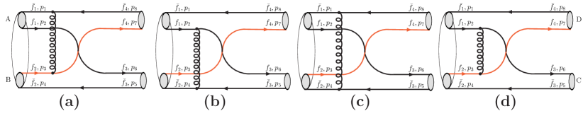
Fig. 1: The four meson-meson scattering diagrams by exchanging $f_{1}f_{2}$ quarks, and similarly by exchanging $\bar{f}_{1}\bar{f}_{1}$ quarks.

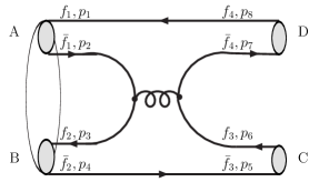
Fig. 2: The schematic diagram for decays of the $K^{*}\bar{K}^{*}$ molecule via a $q\bar{q}$ annihilation.

At hadronic level, the $K^{*}\bar{K}^{*}$ can be scattered into the $\omega\phi$ final sate by exchanging a meson as assumed in [10]. At quark level, such a meson-meson scatterring process has already been investigated by many authors in quark model [11]-[15]. It is found that the process can be described by one gluon exchange (OGE) between $qq$ or $\bar{q}\bar{q}$ pair, by which one found that it gives an excellent description both for the light and heavy meson-meson scattering process. By analogy with these models, we describe the reaction $K^{*}\bar{K}^{*}\to MM$ to begin with the quark-quark scattering, then leads to the quark rearrangement between the two color singlet clusters and subsequent formation of the final two mesons as shown in Fig. 1(a-d). In addition, the $q\bar{q}$ annihilation may take place between $K^{*}$ and $\bar{K}^{*}$ clusters and leads to the $(K^{*}\bar{K}^{*})$ molecule to decay into the different final state as shown in Fig. 2.

As the $K^{*}\bar{K}^{*}$ in the molecule are weakly bound, we may relate this decay rate to the cross section $\sigma(K^{*}\bar{K}^{*}\to M_{1}M_{2})$ near threshold, by analogy with the calculation of the decay rate of ${}^{1}S_{0}$ positronium to $\gamma\gamma$. The decay rate for a $(K^{*}\bar{K}^{*})$-molecule is [22]:

$$\Gamma((K^{*}\bar{K}^{*})\to M_{1}M_{2})=\sigma(K^{*}\bar{K}^{*}\to M_{1}M_{2})\cdot v_{rel}\cdot|\Psi_{(K^{*}\bar{K}^{*})}(0)|^{2},$$ (2)

where $v_{rel}$ is the relative velocity of the $K^{*}$ and $\bar{K}^{*}$, $\Psi_{(K^{*}\bar{K}^{*})}(0)$ is the $(K^{*}\bar{K}^{*})$-molecule wavefunction at the origin ${\bf r}=0$. The cross section can be expressed by the invariant amplitudes for the scattering of $K^{*}\bar{K}^{*}$ to the final meson pair, i.e.

$${d\sigma((K^{*}\bar{K}^{*})\to M_{1}M_{2})\over dt}={1\over 64\pi s^{2}}{1\over|P_{Acm}|^{2}}|\mathcal{M}((K^{*}\bar{K}^{*})\to M_{1}M_{2})|^{2},$$ (3)

where the Mandlestam variable $t=M_{A}^{2}-2E_{A}E_{C}+2{\bf P_{A}\cdot P_{C}}+M_{C}^{2}$. The invariant amplitude $\mathcal{M}$ is generally expressed as:

$$\mathcal{M}=\langle M_{1}M_{2}|H_{I}|(K^{*}\bar{K}^{*})\rangle=F_{\textrm{color}}F_{\textrm{flavor}}F_{\textrm{spin+space}}$$ (4)

For the quark-exchange mechanism and the quark-annihilation mechanism, on has $F_{\textrm{color}}=4/9$.

The flavor factors are calculated based on the flavor functions of the final meson pairs with the interaction $H_{f}$, which can be written as, for example,

$$H_{f}=\left\{\begin{array}[]{lr}\delta_{f_{1}f_{3}}\delta_{f_{2}f_{4}}\delta_{\bar{f}_{1}\bar{f}_{4}}\delta_{\bar{f}_{2}\bar{f}_{3}}&\textrm{ for Fig. \ref{exch} (a)},\\ a^{+}_{\bar{f}_{4}}a^{+}_{f_{3}}a_{\bar{f}_{1}}a_{f_{2}}&\textrm{ for Fig. \ref{anni} }.\end{array}\right.$$ (5)

where $f$ denotes quark flavor, $a^{+}_{f}$ and $a_{f}$ are the quark $f$ creation and annihilation operator, respectively.

The contributions from the spin and space parts are denoted by:

$$F_{\textrm{spin+space}}=\langle\varphi_{M_{1}}\varphi_{M_{2}}|H_{ss}|\varphi_{K^{*}}\varphi_{\bar{K}^{*}}\rangle,$$ (6)

where $\varphi_{M}$ and $\varphi_{K^{*}}$ denote the wave functions of the decayed mesons and $K^{*}$ molecular state in spin and coordinate space, respectively. They are directly evaluated by Feynman diagrams as shown in Fig. 1 and Fig. 2. It reads:

$$F_{\textrm{spin+space}} = {1\over(2\pi)^{6}}\int\left[\prod_{i=1}^{8}d^{3}{\bf p}_{i}\right]\mathcal{H}~{}\varphi_{K^{*}}({\bf p_{1}-p_{2}})\varphi_{\bar{K}^{*}}({\bf p_{3}-p_{4}})\varphi_{\bar{M}_{1}}({\bf p_{5}-p_{6}})\varphi_{M_{2}}({\bf p_{7}-p_{8}})$$ (7)

$$\times \delta^{3}({\bf P_{A}-p_{1}-p_{2}})\delta^{3}({\bf P_{B}-p_{3}-p_{4}})\delta^{3}({\bf P_{C}-p_{5}-p_{6}})\delta^{3}({\bf P_{D}-p_{7}-p_{8}}),$$

For the quark $f_{1}f_{2}$ exchange mode (Fig. 1), the operator $\mathcal{H}$ reads:

$$\mathcal{H}_{ex}^{(a)}={1\over(p_{7}-p_{3})^{2}}\bar{v}(s_{1},p_{1})\gamma_{\mu}v(s_{8},p_{8})\bar{u}(s_{7},p_{7})\gamma^{\mu}u(s_{3},p_{3})\delta_{s_{4},s_{5}}\delta_{s_{2},s_{6}}\delta^{3}({\bf p_{4}-p_{5}})\delta^{3}({\bf p_{2}-p_{6}}),$$ (8)

$$\mathcal{H}_{ex}^{(b)}={1\over(p_{6}-p_{3})^{2}}\bar{v}(s_{4},p_{4})\gamma_{\mu}v(s_{5},p_{5})\bar{u}(s_{6},p_{6})\gamma^{\mu}u(s_{2},p_{2})\delta_{s_{2},s_{7}}\delta_{s_{1},s_{8}}\delta^{3}({\bf p_{2}-p_{7}})\delta^{3}({\bf p_{1}-p_{8}}),$$ (9)

$$\mathcal{H}_{ex}^{(c)}={1\over(p_{5}-p_{4})^{2}}\bar{v}(s_{1},p_{1})\gamma_{\mu}v(s_{8},p_{8})\bar{v}(s_{4},p_{4})\gamma^{\mu}v(s_{5},p_{5})\delta_{s_{2},s_{6}}\delta_{s_{3},s_{7}}\delta^{3}({\bf p_{2}-p_{6}})\delta^{3}({\bf p_{3}-p_{7}}),$$ (10)

$$\mathcal{H}_{ex}^{(d)}={1\over(p_{6}-p_{2})^{2}}\bar{u}(s_{6},p_{6})\gamma_{\mu}u(s_{2},p_{2})\bar{u}(s_{7},p_{7})\gamma^{\mu}u(s_{3},p_{3})\delta_{s_{1},s_{8}}\delta_{s_{4},s_{5}}\delta^{3}({\bf p_{1}-p_{8}})\delta^{3}({\bf p_{4}-p_{5}}),$$ (11)

where $u(s_{i},p_{i})$ and $v(s_{i},p_{i})$ are the quark and antiquark Dirac spinor with the normalization condition $u^{\dagger}(s,p)u(s,p)=-v^{\dagger}(s,p)v(s,p)=2p^{0}$. For the quark $\bar{f}_{1}\bar{f}_{2}$ exchange mode, it has the same diagram and the operator $\mathcal{H}_{ex}$ takes the similar form.

For the quark $\bar{f}_{1}f_{2}$ and $f_{1}\bar{f}_{2}$ annihilation mode (Fig. 2), the interaction $\mathcal{H}$ are respectively given by:

$$\mathcal{H}_{an}^{\bar{f}_{1}f_{2}}={1\over(p_{2}+p_{3})^{2}}\bar{v}(s_{7},p_{7})\gamma_{\mu}u(s_{6},p_{6})\bar{u}(s_{3},p_{3})\gamma^{\mu}v(s_{2},p_{2})\delta_{s_{1},s_{8}}\delta_{s_{4},s_{5}}\delta^{3}({\bf p_{1}-p_{8}})\delta^{3}({\bf p_{4}-p_{5}}),$$ (12)

$$\mathcal{H}_{an}^{f_{1}\bar{f}_{2}}={1\over(p_{1}+p_{4})^{2}}\bar{u}(s_{1},p_{1})\gamma_{\mu}v(s_{4},p_{4})\bar{v}(s_{5},p_{5})\gamma^{\mu}u(s_{8},p_{8})\delta_{s_{2},s_{7}}\delta_{s_{3},s_{6}}\delta^{3}({\bf p_{2}-p_{7}})\delta^{3}({\bf p_{3}-p_{6}}),$$ (13)

3 Production Mechanism

The production of the molecule $(K^{*}\bar{K}^{*})$ is assumed via the $J/\psi$ radiative decay into a real photon ($\gamma$) plus two virtual gluons ($gg$), followed by the formation of the meson pair of $K^{*}\bar{K}^{*}$, and then possible formation of the $K^{*}\bar{K}^{*}$ molecule through the final state interactions occurs. To note that the decay $J/\psi\to\gamma K^{*}\bar{K}^{*}$ has a large branching fraction (Br=$(4.0\pm 1.3)\times 10^{-3})$, then the interactions between the $K^{*}\bar{K}^{*}$ pair may take place and may give birth to the $(K^{*}\bar{K}^{*})$ molecule.

Fig. 3: The schematic diagram for the production of the $(K^{*}\bar{K}^{*})$ molecule in $J/\psi$ radiative decays.

To evaluate the production rate of $(K^{*}\bar{K}^{*})$-molecule, we consider the process as shown in Fig. 3 at the level of the leading order of perturbative QCD, and the bound states are phenomenologically described by their wavefunctions. The whole amplitude can be decomposed into two parts as done in [23, 24], which is written as

$$A=\sum{1\over k_{1}^{2}k_{2}^{2}}\langle J/\psi|\gamma gg\rangle\langle gg|(K^{*}\bar{K}^{*})\rangle,$$ (14)

where $k_{1}$ and $k_{2}$ are the momentum of the two virtual off-shell gluons. The matrix elements of $\langle J/\psi|\gamma gg\rangle$ and $\langle gg|(K^{*}\bar{K}^{*})\rangle$ describes the subprocess $J/\psi\to\gamma gg$ and $gg\to(K^{*}\bar{K}^{*})$, respectively. The sum is over the polarization vectors of the two gluons.

For the subprocess $J/\psi(E)\to\gamma(\epsilon,k)g(\epsilon_{1},k_{1})g(\epsilon_{2},k_{2})$, the amplitude can be expressed by [23]:

$$A^{\psi\to\gamma gg}_{\alpha\nu\nu_{1}\nu_{2}}E^{\alpha}\epsilon^{*\nu}\epsilon^{*\nu_{1}}_{1}\epsilon^{*\nu_{2}}_{2}=8i{R_{\psi}(0)\over\sqrt{4\pi M^{3}}}{M^{2}a_{v}\over(k_{1}+k_{2})\cdot k(k+k_{1})\cdot k_{2}(k+k_{2})\cdot k_{1}},$$ (15)

with

$$a_{v} = \{\epsilon_{1}^{*}\cdot\epsilon_{2}^{*}[-k_{1}\cdot k\epsilon\cdot k_{2}E\cdot k_{1}-k_{2}\cdot k\epsilon^{*}\cdot k_{1}E\cdot k_{2}-k_{1}\cdot kk_{2}\cdot kE\cdot\epsilon^{*}]$$ (16)

$$+ E\cdot\epsilon^{*}[k_{1}\cdot k\epsilon_{1}^{*}\cdot k_{2}\epsilon_{2}\cdot k+k_{2}\cdot k\epsilon_{2}^{*}\cdot k_{1}\epsilon_{1}^{*}\cdot k-k_{1}\cdot k_{2}\epsilon_{1}^{*}\cdot k\epsilon_{2}^{*}\cdot k]\}$$

$$+ \{\epsilon_{1},k_{1}\leftrightarrow\epsilon,k\}+\{\epsilon_{2},k_{2}\leftrightarrow\epsilon,k\},$$

where $E,\epsilon_{1}$ and $\epsilon_{2}$ are polarization vectors for $J/\psi$, the real photon and the two virtual gluons, respectively, and their momentum are denoted by $k,k_{1}$ and $k_{2}$, respectively. $R_{\psi}(0)$ is the $J/\psi$ radial wave function at origin in coordinate space.

For the subprocess $g(\epsilon_{1},k_{1})g(\epsilon_{2},k_{2})\to K^{*}(\epsilon_{K^{*}},P_{2})\bar{K}^{*}(\epsilon_{\bar{K}^{*}},P_{2})$, the amplitude can be directly calculated from the leading-order diagram as shown in Fig. 3 by using the standard Feymman rules. The details of the calculation are given in appendix A. The amplitude is calculated to be:

$$A_{gg\to K^{*}\bar{K}^{*}}^{\mu_{1},\mu_{2}}\epsilon_{1\mu_{1}}\epsilon_{2\mu_{2}} = {1\over 2}{1\over 4\sqrt{p_{1}^{0}p_{2}^{0}q_{1}^{0}q_{2}^{0}}}{1\over\sqrt{(q_{1}^{0}+m_{s})(q_{2}^{0}+m_{s})(p_{1}^{0}+m_{u})(p_{2}^{0}+m_{u})}}{R_{K^{*}}^{2}(0)\over 4\pi}$$ (17)

$$\times \textrm{Tr}[(-q\!\!\!/_{1}+m_{s})\epsilon\!\!\!/_{K^{*}}(p\!\!\!/_{1}+m_{u})\epsilon\!\!\!/_{2}(-q\!\!\!/_{2}+m_{s})\epsilon_{\bar{K}^{*}}(p\!\!\!/_{2}+m_{u})\epsilon\!\!\!/_{1}$$

$$+ (\epsilon_{1}\leftrightarrow\epsilon_{2})],$$

where $R_{K^{*}}(0)$ is the $K^{*}$ wave function at origin, and $p_{1}$ and $q_{1}$ are respectively the momentum of $u-$quark and $s-$quark bound in $K^{*}$, and the antiparticle counterparts denoted by $p_{2}$ and $q_{2}$ with $p_{i}=m_{u}P_{i}/(m_{s}+m_{u})$ and $q_{i}=m_{s}P_{i}/(m_{s}+m_{u})$.

If we assume the $K^{*}\bar{K}^{*}$ pair to be a molecular state, which is phenomenologically described by a wavefunction $\Phi(\bf P_{1}-P_{2})$ given in Eq. (1), then the amplitude for $gg\to(K^{*}\bar{K}^{*})$ reads:

$$A_{gg\to(K^{*}\bar{K}^{*})}^{\mu_{1},\mu_{2}}\epsilon_{1\mu_{1}}\epsilon_{2\mu_{2}}=\int{d^{3}{\bf q}\over\sqrt{2q^{0}(2\pi)^{3}}}A^{gg\to K^{*}\bar{K}^{*}}_{\mu_{1},\mu_{2}}\epsilon_{1\mu_{1}}\epsilon_{2\mu_{2}}{\Psi_{(K^{*}\bar{K}^{*})}(\bf q)},$$ (18)

After inserting Eq. (15) and (17) into Eq. (14), and making substitution $k_{1}=p_{1}+q_{2}$ and $k_{2}=p_{2}+q_{1}$, one obtains the amplitude for $J/\psi\to\gamma K^{*}\bar{K}^{*}$. Using the standard formula for three-body decays [16], the decay width for $J/\psi\to\gamma K^{*}\bar{K}^{*}$ is written as:

$$\Gamma={(2\pi)^{4}\over M_{\psi}}\sum^{-\!\!-}\int\left|{g_{\nu_{1}\mu_{1}}g_{\nu_{2}\mu_{2}}\over(p_{1}+q_{2})^{2}(p_{2}+q_{1})^{2}}A_{\psi\to\gamma gg}^{\alpha\nu\nu_{1}\nu_{2}}E_{\alpha}\epsilon^{*}_{\nu}A_{gg\to K^{*}\bar{K}^{*}}^{\mu_{1},\mu_{2}}\right|^{2}d\phi_{3},$$ (19)

where $\phi_{3}$ is a standard 3-body phase space factor.

Similarly, the decay width for $J/\psi\to\gamma(K^{*}\bar{K}^{*})$ is written as:

$$\Gamma={1\over 8\pi}\sum^{-\!\!-}\left|{g_{\nu_{1}\mu_{1}}g_{\nu_{2}\mu_{2}}\over(p_{1}+q_{2})^{2}(p_{2}+q_{1})^{2}}A_{\psi\to\gamma gg}^{\alpha\nu\nu_{1}\nu_{2}}E_{\alpha}\epsilon^{*}_{\nu}A_{gg\to(K^{*}\bar{K}^{*})}^{\mu_{1},\mu_{2}}\right|^{2}{|{\bf P_{\gamma}}|\over M_{\psi}^{2}},$$ (20)

where ${\bf P_{\gamma}}$ is the photon momentum.

4 Numerical Results

To evaluate the $(K^{*}\bar{K}^{*})$ molecule decay width and the production rate, one should have a reliable method to describe the wavefunctions of the low lying mesons. However, no rigorous theory from the QCD first principle is available to describe the light bound states, so one has to use a phenomenological model to include the nonperturbative properties. Phenomenologically, we construct meson wave functions in the constituent quark model; they are decomposed into three parts, i.e. the flavor, spin and the space wavefunctions. For example, the wave function of $K^{*+}$ is constructed as:

$$|K^{*+}\rangle=|u\bar{s}\rangle\epsilon(1,m)\varphi({\bf p}),$$ (21)

where $\epsilon(1,m)$ denotes the symmetry spin wave function of two constituent quarks. For pseudoscalar mesons, it is chosen as asymmetric spin wave functions.

For $\eta$ and $\eta^{\prime}$ mesons, we choose the mixing scheme to expand their flavor functions in terms of the singlet and octet quark flavor basis as:

$$|\eta\rangle = \cos\phi|\eta_{q}\rangle-\sin\phi|\eta_{s}\rangle,$$

$$|\eta^{\prime}\rangle = \sin\phi|\eta_{q}\rangle+\cos\phi|\eta_{s}\rangle,$$ (22)

where $\phi$ is the mixing angle, $|\eta_{q}\rangle=|u\bar{u}+d\bar{d}\rangle/\sqrt{2}\varphi_{q}({\bf p})$ and $|\eta_{s}\rangle=|s\bar{s}\rangle\varphi_{s}({\bf p})$, where $\varphi({\bf p})$ is chosen as the ground harmonic oscillator basis associated with the decay constant $f_{q}$ or $f_{s}$. In [25] the mixing angle and the decay constants are extracted from the experimental data as: $\phi=39.3^{\circ}\pm 1.0^{\circ},~{}f_{q}=(1.07\pm 0.02)f_{\pi}$ and $f_{s}=(1.34\pm 0.06)f_{\pi}$. The flavor factors for $X(1812)\to\eta\eta^{\prime},~{}\eta\eta$, together with the other final states, are given in Table 1.

The space wave function $\varphi({\bf p})$ is solely dependent on the harmonic oscillator parameter $\beta$. From some studies on the the spectroscopy and decay rates of the low lying scalar and vector mesons, their decay constant is determined; they are related to the meson wavefunction at the origin by $f_{P,V}=\sqrt{12\over M_{P,V}}|\phi_{P,V}(0)|$. On the other hand, the wave function at the origin is related to the parameter $\beta$ by $\phi_{P,V}(0)=(\beta^{2}/\pi)^{3/4}$. Table 2 summarizes the decay constants determined by experimental data [26] and the harmonic oscillator parameters determined by the relation $\beta_{P,V}=\sqrt{\pi}({M\over 12})^{1/3}f_{P,V}^{2/3}$.

Tab. 1: The flavor factor for the $K^{*}\bar{K}^{*}$ molecule decays into a meson pair via the quark exchange and annihilation mechanism.

	Annihilation		Exchange
$M_{1}M_{2}$	$s\bar{s}\to u\bar{u}$	$u\bar{u}\to s\bar{s}$	$s\leftrightarrow u$ or $\bar{s}\leftrightarrow\bar{u}$
$\omega\omega$	1/2	0	0
$\rho^{+}\rho^{-}$	1	0	0
$\omega\phi$	0	0	$1/\sqrt{2}$
$K^{*+}K^{*-}$	1	1	0
$\eta\eta$	$\cos^{2}\phi/2$	$\sin^{2}\phi$	$-\sqrt{2}\sin 2\phi$
$\eta\eta^{\prime}$	$\sin 2\phi/4$	$-\sin^{2}\phi/2$	$\cos 2\phi/\sqrt{2}$
$\pi^{+}\pi^{-}$	$1/2$	$0$	$0$
$K^{+}K^{-}$	$s\bar{s}\to s\bar{s}:1$	$u\bar{u}\to u\bar{u}:1$	$0$

Tab. 2: The harmonic parameters calculated with the mass $M$ and the decay constant $f_{M}$ [26] by the relation $\beta=\sqrt{\pi}({M\over 12})^{1/3}f_{M}^{2/3}$

Meson	Mass (GeV)	$f_{M}$	$\beta$ (GeV)
$\pi$	$m_{\pi}$	$f_{\pi}=0.130$	0.103
$\eta_{q}$	$m_{\pi}$	$1.07f_{\pi}$	0.108
$\eta_{s}$	$\sqrt{2m_{K}^{2}-m_{\pi}^{2}}$	$1.34f_{\pi}$	0.213
$\rho$	$m_{\rho}$	$0.220$	0.258
$\omega$	$m_{\omega}$	$0.195$	0.240
$K$	$m_{K}$	$0.159$	0.180
$\phi$	$m_{\phi}$	$0.245$	0.305
$K^{*}$	$m_{K^{*}}$	$0.217$	0.270

For $X(1812)\to M_{1}M_{2}$ decays, the decay width includes the contributions from the quark exchange and quark annihilation mechanisms, respectively denoted by $\Gamma_{M_{1}M_{2}}^{\textrm{ex}}$ and $\Gamma_{M_{1}M_{2}}^{\textrm{an}}$ . Due to the non-zero flavor factors, the quark exchange mechanism allows only three decays, $\omega\phi,~{}\eta\eta$ and $\eta\eta^{\prime}$ channels as shown in Table 1. The calculation of the decay width is straightforward though tedious according to Eq. (3). The numerical calculation yields the ratios:

$$\Gamma_{\eta\eta^{\prime}}^{\textrm{ex}}:\Gamma_{\eta\eta}^{\textrm{ex}}:\Gamma_{\omega\phi}^{\textrm{ex}}:\Gamma_{K^{+}K^{-}}^{\textrm{ex}}:\Gamma_{\rho^{+}\rho^{-}}^{\textrm{ex}}:\Gamma_{\omega\omega}^{\textrm{ex}}:\Gamma_{K^{*+}K^{*-}}^{\textrm{ex}}:\Gamma_{\pi^{+}\pi^{-}}^{\textrm{ex}}=$$

$$9.3:4.3:1.0:0:0:0:0:0.$$ (23)

This indicates that the quark exchange mechanism enhances the decays $X(1812)\to\eta\eta$ and $\eta\eta^{\prime}$. On the other hand, the quark annihilation mechanism makes no contribution to the decay $X(1812)\to\omega\phi$. To determine the contributions from this mechanism, we estimate the reduced ratios $\tilde{\Gamma}_{M_{1}M_{2}}^{\textrm{an}}=\Gamma_{M_{1}M_{2}}^{\textrm{an}}/\Gamma_{\omega\phi}^{\textrm{ex}}$. The numerical calculation yields:

$$\tilde{\Gamma}_{\eta\eta^{\prime}}^{\textrm{an}}:\tilde{\Gamma}_{\eta\eta}^{\textrm{an}}:\tilde{\Gamma}_{\omega\phi}^{\textrm{an}}:\tilde{\Gamma}_{K^{+}K^{-}}^{\textrm{an}}:\tilde{\Gamma}_{\rho^{+}\rho^{-}}^{\textrm{an}}:\tilde{\Gamma}_{\omega\omega}^{\textrm{an}}:\tilde{\Gamma}_{K^{*+}K^{*-}}^{\textrm{an}}:\tilde{\Gamma}_{\pi^{+}\pi^{-}}^{\textrm{an}}=$$

$$0.39:0.04:0:0.44:0.41:0.005:0.001:1.9\times 10^{-5}.$$ (24)

This indicates that the quark annihilation mechanism makes small contributions to $X(1812)\to M_{1}M_{2}$, especially for the $\pi^{+}\pi^{-}$ mode, which is highly suppressed in dynamics. If the both decay mechanisms and the interference effects between them are taken into consideration, the total decay widths for each mode are calculated to be:

$$\Gamma_{\eta\eta^{\prime}}:\Gamma_{\eta\eta}:\Gamma_{\omega\phi}:\Gamma_{K^{+}K^{-}}:\Gamma_{\rho^{+}\rho^{-}}:\Gamma_{\omega\omega}:\Gamma_{K^{*+}K^{*-}}:\Gamma_{\pi^{+}\pi^{-}}=$$

$$13.6:5.14:1:0.44:0.41:0.005:0.001:1.9\times 10^{-5}$$ (25)

For the production of the $(K^{*}\bar{K}^{*})$ molecule in the $J/\psi\to\gamma(K^{*}\bar{K}^{*})$, the production rate depends on the overlap of the $K^{*}$ and $\bar{K}^{*}$ wave functions in momentum space. They are phenomenologically described by ground harmonic oscillator bases with a parameter $\beta$, which is related to the root mean square (rms) radius $\langle r^{2}\rangle$ by the relation of $\beta=\sqrt{{3\over 2\langle r^{2}\rangle}}$. The model study using a nonrelativistic Hamiltonian with pairwise effective interactions shows that the rms becomes large when the binding energy of two-meson molecule decreases [21]. With the binding energy ranging from $100$ MeV to a few Mev, the rms runs from 0.3fm to $2$ fm. Near the threshold of two bound mesons, the rms of the molecule is about 1-2 fm. In our calculation, we naively set the $\beta$ parameter within the range $0.5\sim 2.0$ fm. From Eq. (19-20) the numerical calculation yields the ratios of the decay width for the $J/\psi\to\gamma K^{*}\bar{K}^{*}$ and $\gamma(K^{*}\bar{K}^{*})$, which are given in Table 3. The results show that the strong binding of the $(K^{*}\bar{K}^{*})$ molecule favors its production from $J/\psi$ decays.

Tab. 3: The production rate of $\Gamma_{\gamma(K^{*}\bar{K}^{*})}/\Gamma_{\gamma K^{*}\bar{K}^{*}}$ in terms of the rms of the $(K^{*}\bar{K}^{*})$ molecule.

$\sqrt{\langle r^{2}\rangle}$fm	0.5	0.8	1	1.5	2.0
$\Gamma_{\gamma(K^{*}\bar{K}^{*})}/\Gamma_{\gamma K^{*}\bar{K}^{*}}$	9.54	3.79	2.13	0.66	0.28

5 Discussion and Summary

Based on the scenario of $X(1812)$ to be a $(K^{*}\bar{K}^{*})$ molecule, the decay width and the production rate are evaluated. It is found that the quark exchange mechanism plays an important role in the understanding of the decay $X(1812)\to\omega\phi$, and we find that this decay mechanism enhances the decay widths for $\eta\eta$ and $\eta\eta^{\prime}$ modes. On the other hand, the quark annihilation mechanism makes a small contributions to $X(1812)\to PP$ and $VV$ decays, and the decay $X(1812)\to\pi\pi$ is highly suppressed in dynamics. These results suggest that if $X(1812)$ is a $(K^{*}\bar{K}^{*})$ molecule, it should be found in the decays $J/\psi\to\gamma X,~{}X\to\eta\eta^{\prime}$ and $\eta\eta$ except for the observed mode $X\to\omega\phi$. Unfortunately, due to the low statistics of the present data sample, no information on $J/\psi\to\gamma\eta\eta^{\prime}$ and $\gamma\eta\eta$ decays are available in PDG table.

Figure 4 shows experimental information on the invariant mass distribution of two mesons in $J/\psi\to\gamma\omega\phi,~{}\gamma\eta\eta,~{}\gamma\rho^{+}\rho^{-},~{}\gamma K^{+}K^{-},~{}\gamma\omega\omega,~{}\gamma K^{*+}K^{*-}$ and $\gamma\pi^{+}\pi^{-}$. In $X(1812)$ mass region as seen in the $J/\psi\to\gamma\omega\phi$, no signal evidence is observed in the other decays. As for the decay $J/\psi\to\gamma\eta\eta$, it is firstly reported by the collaboration of Crystal Ball detector twenty years ago with very low statistics, but after that no confirmation was made by other collaborations. Our predictions deserve to be tested in this decay, together with the $J/\psi\to\gamma\eta\eta^{\prime}$. With a large data sample accumulation and the improvement in the detector performance, especially for the photon identification for BESIII and CLEOc detector, search for $X(1812)$ signals in these two channels are possibly achieved. In the $J/\psi\to\gamma\rho^{+}\rho^{-}$, the partial wave analysis (PWA) shows that the contribution from scalar near the mass of 1690 MeV dominates the $m_{\rho\rho}$ mass distribution. In the $J/\psi\to\gamma\pi^{+}\pi^{-}$, the PWA shows that significant resonance with mass 1270 Mev favors the $J^{PC}=2^{++}$, and small scalar components with mass equal to 1466 MeV and 1765 MeV are also reported. Recently, the BESII collaboration reported the PWA performed on the $J/\psi\to\gamma\omega\omega$. The results show that the contributions in the mass distribution of $m_{\omega\omega}$ below $2.0$ GeV are predominantly from pseudoscalars, and only with small contributions from $f_{0}(1710),~{}f_{2}(1640)$ and $f_{2}(1910)$. The PWA of the decay $J/\psi\to\gamma K^{+}K^{-}$ is also reported by the BESII collaboration, the dominant contributions are from the scalar $f_{0}(1710)$ and the tensor $f_{2}^{\prime}(1525)$. The PWA on the decay $J/\psi\to\gamma K^{*}\bar{K}^{*}$ is reported by BESI collaboration with 7.8 million $J/\psi$ data, the results showed that a broad $0^{-+}$ resonance with mass $M=1800$ MeV is observed, no significant $0^{++},~{}1^{++}$ or $4^{++}$ signal is found. In short, no evidence for $X(1812)$ is currently observed in the hadron mass distributions of the radiative decays: $J/\psi\to\gamma\rho^{+}\rho^{-},~{}\gamma K^{+}K^{-},~{}\gamma\omega\omega,~{}\gamma K^{*+}K^{*-}$ and $\gamma\pi^{+}\pi^{-}$, from which it seems to be consistent with the our calculation based on the $(K^{*}\bar{K}^{*})$ molecular picture. The further test of this scenario is expected to search for the $X(1812)$ in $J/\psi\to\gamma\eta\eta^{\prime}$ and $\gamma\eta\eta$ decays in the future.

Fig. 4: The experimental measurement of mass distributions $m_{h_{1}h_{2}}$ for radiative decays of $J/\psi\to\gamma h_{1}h_{2}$, (a) $J/\psi\to\gamma\omega\phi$[27], (b) $J/\psi\to\gamma\eta\eta$ [28], (c) $J/\psi\to\gamma\rho^{+}\rho^{-}$ [29], (d) $J/\psi\to\gamma K^{+}K^{-}$ [30], (e) $J/\psi\to\gamma\omega\omega$[31], (f) $J/\psi\to\gamma K^{*+}K^{*-}$ [32], (g) $J/\psi\to\gamma\pi^{+}\pi^{-}$ [33].

If we naively assume that the $(K^{*+}K^{*-})$ molecule dominantly decays into $\eta\eta^{\prime},~{}\eta\eta,\omega\phi,~{}K\bar{K}$ and $\rho\rho$, then one obtains $Br(X\to\omega\phi)\simeq 4.60\%$ from our calculations. From the measurement of $Br(J/\psi\to\gamma X)Br(X\to\omega\phi)=(2.61\pm 0.71)\times 10^{-4}$, one has the production rate $Br(J/\psi\to\gamma X)=(5.67\pm 0.07)\times 10^{-3}$. Combined with the PDG value, one has $\Gamma(J/\psi\to\gamma X)/\Gamma(J/\psi\to\gamma K^{*+}K^{*-})=2.83\pm 0.92$. Our calculation yields $\Gamma(J/\psi\to\gamma X)/\Gamma(J/\psi\to\gamma K^{*+}K^{*-})=2.13^{+7.41}_{-1.85}$, where the central value corresponds to the $\sqrt{\langle r^{2}\rangle}=1.0$ fm, and the uncertainty corresponds to the range $0.5\textrm{~{}fm}\leq\sqrt{\langle r^{2}\rangle}\leq 2.0\textrm{~{}fm}$.

It is also important to look for decay rates of $X(1812)\to PP$ and $VV$ in experiment for understanding its nature. Theoretically, these decays have been evaluated numerically by many authors using different models to describe the $X(1812)$ structure. For example, in four-quark picture [9], it is found that $X(1812)\to\omega\omega,~{}K^{*}\bar{K}^{*}$ are the two dominant decay channels and $X(1812)\to K\bar{K},~{}\eta\eta,~{}\eta\eta^{\prime}$ are suppressed. While in glueball picture [5], the dominant decays are $X(1812)\to\rho\rho$ and $\omega\omega$, and decays into $\omega\phi$ and $K^{*}\bar{K}^{*}$ are highly suppressed. In the quarkonia-glueball-hybrid mixing scheme [8], it turns out that the branching fractions for $X(1812)\to K\bar{K}$ and $\eta\eta$ are about 30%, which adds up to about 70% of the total $X(1812)$ decay width. However, in our $(K^{*}\bar{K}^{*})$ molecule picture, the dominate decays are $X(1812)\to\eta\eta^{\prime}$ and $\eta\eta$.

In summary, we evaluate the decay widths of $X(1812)\to\eta\eta^{\prime},~{}\eta\eta,~{}\omega\phi,~{}K^{+}K^{-},~{}\rho^{+}\rho^{-},~{}\omega\omega,~{}K^{*+}K^{*-}$ and $\pi^{+}\pi^{-}$ based on the assumption of the $X(1812)$ as a candidate of $(K^{*}\bar{K}^{*})$ molecule. It turns out that the quark exchange mechanism plays an important role in the understanding of the large decay with for the $X(1812)\to\omega\phi$. We also find that the decay widths for $X(1812)\to\eta\eta^{\prime}$ and $\eta\eta$ decays are enhanced by the quark exchange mechanism. These channels are suggested to be the tools to test the molecular scenario in experiment. The branching fraction of $Br(X\to\omega\phi)$ is evaluated to be about $4.60\%$. Searches for additional evidence about the $X(1812)$ in $J/\psi$ radiative decays are reviewed. In the molecular scenario, the $X(1812)$ production rate is also evaluated to be $\Gamma(J/\psi\to\gamma X)/\Gamma(J/\psi\to\gamma K^{*+}K^{*-})=2.13^{+7.41}_{-1.85}$, which is close to the measured value $2.83\pm 0.92$.

Acknowledgements
The work is partly supported by the National Natural Science Foundation of China under Grant Nos. 10575083, 10435080, 10375074 and 10491303.

Appendix A The amplitude for $gg\to K^{*}\bar{K}^{*}$

We start with the process $g(\epsilon_{1})g(\epsilon_{2})\to q(p_{1},s_{1})\bar{q}(q_{1},\bar{s}_{1})q(p_{2},s_{2})\bar{q}(q_{2},\bar{s}_{2})\to K^{*}({\bf P_{1}})\bar{K}^{*}({\bf P_{2}})$ as shown in Fig. 3, where $\epsilon_{i}~{}(i=1,2)$ denotes the polarization vector of the gluon; the momentum and the spin of the quark (antiquark) $q~{}(\bar{q})$ are denoted by $p_{i}~{}(q_{i})$ and $s_{i}~{}(\bar{s}_{i})$, respectively; the outgoing momentum for $K^{*}~{}(\bar{K}^{*})$ is denoted by ${\bf P_{1}}~{}({\bf P_{2}})$. The amplitude with Lorentz indexes $\mu_{1}$ and $\mu_{2}$ is defined as:

$$A_{gg\to K^{*}\bar{K}^{*}}^{\mu_{1}\mu_{2}} = \int{1\over\sqrt{2p_{1}^{0}2q_{1}^{0}2p_{2}^{0}2p_{2}^{0}}}{d^{3}p_{1}\over(2\pi)^{3}}{d^{3}q_{1}\over(2\pi)^{3}}{d^{3}p_{2}\over(2\pi)^{3}}{d^{3}q_{2}\over(2\pi)^{3}}$$ (26)

$$\times \sum_{\textrm{all spin indexes}}\bar{u}(s_{1},p_{1})\gamma^{\mu_{1}}v(\bar{s}_{2},q_{2})u(s_{2},p_{2})\gamma^{\mu_{2}}v(\bar{s}_{1},q_{1})$$

$$\times \langle{1\over 2}s_{1};{1\over 2}\bar{s}_{1}|S_{1}S_{1z}\rangle\langle{1\over 2}s_{2};{1\over 2}\bar{s}_{2}|S_{2}S_{2z}\rangle\langle L_{1}M_{1};S_{1}S_{1z}|J_{1}J_{1z}\rangle\langle L_{2}M_{2};S_{2}S_{2z}|J_{2}J_{2z}\rangle$$

$$\times \Psi_{K^{*}L_{1}S_{1}}({\bf p_{1}-q_{1}})\Psi_{\bar{K}^{*}L_{2}S_{2}}({\bf p_{2}-q_{2}})$$

$$\times (2\pi)^{3}\delta({\bf P_{1}-p_{1}-q_{1}})(2\pi)^{3}\delta({\bf P_{2}-p_{2}-q_{2}}),$$

where $\Psi_{K^{*}L_{1}S_{1}}~{}(\Psi_{\bar{K}^{*}L_{2}S_{2}})$ denotes the wave function for $K^{*}~{}(\bar{K}^{*})$ with the orbit and spin angular-momentum quantum number $L_{1}~{}(L_{2})$ and $S_{1}~{}(S_{2})$, respectively. For the vector meson $K^{*}$, it is assigned as the ${}^{3}S_{1}$ state in $q\bar{q}$ quark model. So we have $L_{i}=0$ and $S_{i}=J_{iz}=1~{}(i=1,2)$.

The above amplitude can be simplified with the help of the spin projection operator $P_{S_{1}S_{1z};S_{2}S_{2z}}^{\mu_{1}\mu_{2}}$, which is defined as:

$$P_{S_{1}S_{1z};S_{2}S_{2z}}^{\mu_{1}\mu_{2}} \equiv \sum_{s_{1}\bar{s}_{1}s_{2}\bar{s}_{2}}u(s_{1},p_{1})\gamma^{\mu_{1}}v(\bar{s}_{2},q_{2})u(s_{2},p_{2})\gamma^{\mu_{2}}v(\bar{s}_{1},q_{1})$$ (27)

$$\times \langle{1\over 2}s_{1};{1\over 2}\bar{s}_{1}|S_{1}S_{1z}\rangle\langle{1\over 2}s_{2};{1\over 2}\bar{s}_{2}|S_{2}S_{2z}\rangle$$

$$= \textrm{Tr}\left[\sum_{s_{1}\bar{s}_{1}}v(\bar{s}_{1},q_{1})u(s_{1},p_{1})\gamma^{\mu_{1}}\langle{1\over 2}s_{1};{1\over 2}\bar{s}_{1}|S_{1}S_{1z}\rangle\right.$$

$$\times \left.\sum_{s_{2}\bar{s}_{2}}v(\bar{s}_{2},q_{2})u(s_{2},p_{2})\gamma^{\mu_{2}}\langle{1\over 2}s_{2};{1\over 2}\bar{s}_{2}|S_{2}S_{2z}\rangle\right]$$

$$\equiv \textrm{Tr}[P_{1S_{1z}}P_{1S_{2z}}],$$

where $P_{1S_{1z}}$ and $P_{1S_{2z}}$ are the spin projection operators for the spin-1 particles. As given in [34], they are explicitly expressed with the spin polarization vectors $\epsilon_{K^{*}}$ as:

$$P_{1S_{z}}^{\mu}(p_{i},q_{i}) \equiv \sum_{s_{i}\bar{s}_{i}}v(\bar{s}_{i},q_{i})u(s_{i},p_{i})\gamma^{\mu}\langle{1\over 2}s_{i};{1\over 2}\bar{s}_{i}|1S_{z}\rangle$$ (28)

$$= {1\over\sqrt{(q_{i}^{0}+m_{s})(p_{i}^{0}+m_{u})}}(-q\!\!\!/_{i}+m_{s})\epsilon_{K^{*}}(S_{z})(p\!\!\!/+m_{u}).$$

To simplify the integral in Eq. (26), one method to make an approximation is the nonrelativistic assumption for valence quarks, ie. ${\bf p_{i}-q_{i}}=2{\bf q}\rightarrow 0$. Then the integral of the amplitude can be evaluated at the origin with the substitution of the momentum $p_{i}={m_{u}P_{i}\over m_{u}+m_{s}}$ and $q_{i}={m_{s}P_{i}\over m_{u}+m_{s}}$, ie.

$$\int{d^{3}p_{1}\over(2\pi)^{3}}{d^{3}q_{1}\over(2\pi)^{3}}\Psi_{K^{*}0S}({\bf p_{1}-q_{1}})(2\pi)^{3}\delta({\bf P_{1}-p_{1}-q_{1}})\approx{R_{K^{*}0}(0)\over\sqrt{4\pi}},$$ (29)

where $R_{K^{*}0}(0)$ is the radius wavefunction for the $K^{*}$ at origin. With the help of equations (27) to (29), the amplitude for $gg\to K^{*}\bar{K}^{*}$ can be simplified as:

$$A_{gg\to K^{*}\bar{K}^{*}}^{\mu_{1},\mu_{2}}\epsilon_{1\mu_{1}}\epsilon_{2\mu_{2}} = {1\over 2!}{1\over 4\sqrt{p_{1}^{0}p_{2}^{0}q_{1}^{0}q_{2}^{0}}}{1\over\sqrt{(q_{1}^{0}+m_{s})(q_{2}^{0}+m_{s})(p_{1}^{0}+m_{u})(p_{2}^{0}+m_{u})}}{R_{K^{*}}^{2}(0)\over 4\pi}$$ (30)

$$\times \textrm{Tr}[(-q\!\!\!/_{1}+m_{s})\epsilon\!\!\!/_{K^{*}}(p\!\!\!/_{1}+m_{u})\epsilon\!\!\!/_{2}(-q\!\!\!/_{2}+m_{s})\epsilon_{\bar{K}^{*}}(p\!\!\!/_{2}+m_{u})\epsilon\!\!\!/_{1}$$

$$+ (\epsilon_{1}\leftrightarrow\epsilon_{2})],$$

where the factor of $1/2!$ comes from the contribution of the cross term for the two gluons of identical particles.

References

• [1] Ablikim M et al (BES Collaboration) 2006 Phys. Rev. Lett. 96 162002.
• [2] Close F E and Tornqvist N A 2002 J. Phys. G 28 R249.
• [3] Amsler C and Close F E 2004 Phys. Rep. 389 61.
• [4] Horn D and Mandula J 1978 Phys. Rev. D 17 898.
• [5] Bicudo P, Cotanch S R, Llanes-Estrada F J, and Robertson D G 2006 Preprint hep-ph/0602172.
• [6] Bugg D V 2006 Preprint hep-ph/0603018.
• [7] Chao K T 2006 Preprint hep-ph/0602190.
• [8] He X G, Li X Q, Liu X, and Zeng X Q 2006 Phys. Rev. D 73 114026.
• [9] Li B A 2006 Phys. Rev. D 74 054017.
• [10] Zhao Qiang and Zou Bing-Son 2006 Phys. Rev. D 74 114025.
• [11] Barnes T, Black N, Dean D J and Swanson E S 1999 Phys. Rev. C 60 045202.
• [12] Barnes T, Black N and Swanson E S 2001 Phys. Rev. C 63 025204.
• [13] Barnes T and Swanson E S 1992 Phys. Rev. D 46, 131; Zhao G Q, Jing X G, and Su J C 1998 Phys. Rev. 58 117503; Blaschke D and Ropke G 1993 Phys. Lett. B 299 332; Martins K, Blaschke D, and Quack E 1995 Phys. Rev. C 51 2723.
• [14] Swanson E S 1992 Ann. Phys. 220 73.
• [15] Barnes T, Swanson E S, and Weinstein J 1992 Phys. Rev. D 46 4868.
• [16] Yao W M et al 2006 2006 J. Phys. G 33 1.
• [17] Jaffe R J 1997 Phys. Rev. D 15 267; 1997 Phys. Rev. 15 281.
• [18] Donoghue J F 1985 HADRON’1985 edited by S. Oneda, AIP Conf. Proc. No. 132 (AIP, New York, 1985), p.460.
• [19] Weinstein J and Isgur N 1983 Phys. Rev. D 27 588; 1990 Phys. Rev. 41 2336; 1991 Phys. Rev. 43 95.
• [20] Chen Jian-Xing Ying-Hui Cao and Jun-Chen Su 2001 Phys. Rev. C 64 065201.
• [21] Wong Cheuk-Yin 2004 Phys. Rev. C 69 055202.
• [22] Stroscio M A 1975 Phys. Rept. 22 215;
Barnes T 1985 Phys. Lett. B 165 434;
Shmatikov M 1996 Nucl. Phys. A 596 425.
• [23] Korner J G, Kuhn J H, Krammer M and Heniz Scheneider 1983 Nucl. Phys. B 229 115.
• [24] Close F E, Farrar G R and Li z 1997 Phys. Rev. D 55 5749.
• [25] Feldmann Th, Kroll P and Stech B 1988 Phys. Rev. D58 114006.
• [26] Yao W M et. al. 2006 J. Phys. G 2006 33 1;
Ebert D, Faustov R N, Galkin V O 2006 Phys. Lett. B 635 93.
• [27] Ablikim M, et. al. BES collaboration 2006 Phys. Rev. Lett. 96 162002.
• [28] Elliott D Bloom and Charles W Peck 1983 Ann. Rev. Nucl. Part. Sci. 33 143.
• [29] Baltrusaitis R M, et. al. Mark III collaboration 1986 Phys. Rev. D 33 1222.
• [30] J Z Bai, et. al. BES collaboration 2003 Phys. Rev. D 68 052003.
• [31] Ablikim M, et. al. BES collaboration 2006 Phys. Rev. D 73 112007.
• [32] Bai J Z, et. al. BES collaboration 2000 Phys. Lett. B 472 200.
• [33] Ablikim M, et. al. BES collaboration 2006 Phys. Lett. B 642 441.
• [34] Giberoma B, Kuhn J H, Peccei R D and Ruckl R 1980 Nucl. Phys. B 174 317.