Relations between generalized and
transverse momentum dependent parton distributions

Abstract

Recent work suggests nontrivial relations between generalized parton distributions on the one hand and (naive time-reversal odd) transverse momentum dependent distributions on the other. Here we review the present knowledge on such type of relations. Moreover, as far as spectator model calculations are concerned, the existing results are considerably extended. While various relations between the two types of parton distributions can be found in the framework of spectator models, so far no nontrivial model-independent relations have been established.

I Introduction

For decades the partonic structure of the nucleon was almost entirely discussed in terms of unpolarized and polarized forward parton densities, which merely depend on the longitudinal momentum of the respective parton. A much more comprehensive picture of the nucleon structure, however, can be obtained by considering two other, more general types of parton distributions: first, generalized parton distributions (GPDs) entering the QCD description of hard exclusive reactions on the nucleon (see, e.g., Refs. Mueller et al. (1994); Diehl (2003); Belitsky and Radyushkin (2005)); second, transverse momentum dependent parton distributions (TMDs) entering the description of various hard semi-inclusive reactions (see, e.g., Ref. Barone et al. (2002); Mulders and Tangerman (1996); Bacchetta et al. (2007)). Not only a large body of theoretical work on these types of parton correlators appeared during the last decade, but also new high luminosity particle accelerators nowadays allow one to explore such intriguing though complicated objects experimentally.

On the TMD side the so-called naive time-reversal odd (T-odd) parton distributions are of particular importance, because these objects can give rise to single spin asymmetries (SSAs). Single spin phenomena were measured in hadron-hadron collisions at FermiLab Adams et al. (1991a, b) and at RHIC Adams et al. (2004); Adler et al. (2005), as well as in lepton-hadron collisions by the COMPASS Collaboration Alexakhin et al. (2005); Ageev et al. (2007), the HERMES Collaboration Airapetian et al. (2000, 2001, 2003); Airapetian et al. (2005a, b); Diefenthaler (2005); Airapetian et al. (2007), and at JeffersonLab Avakian et al. (2004). In general, the theoretical description of such observables in the framework of QCD has been and still is a challenge for the theory. However, a crucial step forward was the observation that time-reversal invariance of the strong interaction does not forbid the existence of T-odd TMDs Collins (2002); Brodsky et al. (2002a). At least for the SSAs in lepton-induced reactions a QCD-factorization formula containing T-odd TMDs has been put forward in the meantime Ji et al. (2005, 2004); Collins and Metz (2004).

An important object in this context is the T-odd Sivers function Sivers (1990, 1991), denoted by $f_{1T}^{\perp}$ in the nomenclature of Ref. Boer and Mulders (1998). The Sivers function quantifies the SSA related to the transverse momentum dependent distribution of unpolarized partons inside a transversely polarized target. Experimentally $f_{1T}^{\perp}$ can be studied, e.g., by measuring a transverse SSA in semi-inclusive deep-inelastic scattering (SIDIS). Extractions of the Sivers function from existing SIDIS data Airapetian et al. (2005a); Diefenthaler (2005); Alexakhin et al. (2005); Ageev et al. (2007) have already been performed Efremov et al. (2005); Anselmino et al. (2005a, b); Vogelsang and Yuan (2005); Collins et al. (2006); Anselmino et al. (2005c).

An intuitive picture of various transverse SSAs, in particular, also of the Sivers effect, was proposed in Refs. Burkardt (2002, 2004a). That work suggested for the first time that there may be a close connection between a certain GPD, typically denoted by $E$ (see, e.g., Ref. Diehl (2003)), and the Sivers asymmetry. In order to generate the Sivers effect in SIDIS two ingredients are required in the picture of Refs. Burkardt (2002, 2004a): first, the impact parameter distribution of unpolarized quarks in a transversely polarized target has to be distorted. Such a distortion is directly connected to the GPD $E$. Second, the fragmenting struck quark in SIDIS has to experience a final state interaction with the target spectators.

Though the work in Burkardt (2002, 2004a) provided a very attractive explanation of the origin of the Sivers effect, it did not provide a quantitative connection between the GPD $E$ and $f_{1T}^{\perp}$. For a particular moment of the Sivers function such a connection was later on established in a perturbative low order calculation using a simple diquark spectator model of the nucleon Burkardt and Hwang (2004). Another step forward was made by comparing the correlator for chiral-odd GPDs in impact parameter space on the one hand with the correlator for chiral-odd TMDs on the other Diehl and Hägler (2005). The work Diehl and Hägler (2005) suggested, in particular, a relation between the second leading twist T-odd quark TMD, the Boer-Mulders function $h_{1}^{\perp}$ Boer and Mulders (1998), and a certain linear combination of GPDs. This possible connection between $h_{1}^{\perp}$ and GPDs was afterwards discussed in more detail in Ref. Burkardt (2005). In the framework of the diquark spectator model quite recently another relation between the GPD $E$ and the Sivers function was obtained Lu and Schmidt (2007), which is similar to the one found in Burkardt and Hwang (2004).

Despite these developments so far no nontrivial model-independent relations between GPDs and TMDs have been established. (An attempt in this direction was made, e.g., in Ref. Burkardt (2004a).) If one considers for instance the Sivers function, the crucial problem lies in the fact that there is apparently no model-independent factorization of $f_{1T}^{\perp}$ into a distortion effect, described by the GPD $E$ in impact parameter space, times a final state interaction.

The manuscript is organized in the following way. In Sec. II we give our definitions of the GPDs, both in momentum and in impact parameter space, and of the TMDs. In particular, we also include the gluon sector which so far in the literature has not been discussed at all in the context of possible relations between GPDs and TMDs. Section III is devoted to model-independent considerations of the relations between GPDs and TMDs. Here the current knowledge on this point is summarized and the main difficulties are presented. Also new possible relations for gluon parton distributions are provided, which later on in the manuscript are investigated in a model calculation. Section IV describes model results on relations between GPDs and TMDs, where we exploit two perturbative models for the target: the scalar diquark spectator model of the nucleon, and a quark target model treated in perturbative QCD. The latter, in particular, allows one to study the gluon sector. The model results of the various parton distributions, calculated to lowest nontrivial order in perturbation theory, show relations in accordance with the considerations in Sec. III. In the framework of the two models also on the quark sector new relations are established. Some of these relations contain the results of Ref. Burkardt and Hwang (2004) and of Ref. Lu and Schmidt (2007) as limiting cases. In this section we also argue that even in the context of spectator models certain nontrivial relations between GPDs and TMDs are far from being obvious if one considers higher orders in perturbation theory. Our summary is given in Sec. V. The results on the various parton distributions in the two target models are collected in two appendices.

II Definition of parton distributions

II.1 Generalized parton distributions (GPDs)

We start by presenting the definitions of the GPDs. Unless stated otherwise we follow here the conventions of Ref. Diehl (2003). The momenta of the incoming and outgoing nucleon are given by (see also Fig. 1)

$$p=P-\tfrac{1}{2}\Delta\,,\qquad p^{\prime}=P+\tfrac{1}{2}\Delta\,,$$ (1)

and satisfy $p^{2}=p^{\prime 2}=M^{2}$, with $M$ denoting the nucleon mass. The GPDs depend on the three variables

$$x=\frac{k^{+}}{P^{+}}\,,\qquad\xi=-\frac{\Delta^{+}}{2P^{+}}\,,\qquad t=\Delta^{2}\,,$$ (2)

where the light-cone coordinates are defined by

$$v^{\pm}=\tfrac{1}{\sqrt{2}}(v^{0}\pm v^{3})\,,\qquad\vec{v}_{T}=(v^{1},v^{2})$$ (3)

for a generic 4-vector $v$. In a physical process the so-called skewness $\xi$ and the momentum transfer $t$ to the nucleon are fixed by the external kinematics, whereas $x$ is typically an integration variable. It is convenient to define the following tensors,

$$\delta_{T}^{ij}=-g^{ij}\,,\qquad\epsilon_{T}^{ij}=\epsilon^{-+ij}\,.$$ (4)

Moreover, we use the conventions

$$\epsilon^{0123}=1\,,$$ (5)

$$\gamma_{5}=i\gamma^{0}\gamma^{1}\gamma^{2}\gamma^{3}\,,$$ (6)

$$\sigma^{\mu\nu}=\tfrac{i}{2}(\gamma^{\mu}\gamma^{\nu}-\gamma^{\nu}\gamma^{\mu})\,.$$ (7)

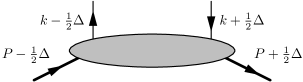
Figure 1: Kinematics for GPDs.

The quark GPDs are defined through the light-cone correlation function

$$F^{q[\Gamma]}(x,\Delta;\lambda,\lambda^{\prime})$$

$$\ =\frac{1}{2}\int\frac{dz^{-}}{2\pi}\,e^{ik\cdot z}\,\big{<}p^{\prime};\lambda^{\prime}\big{|}\,\bar{\psi}\big{(}\!-\!\tfrac{1}{2}z\big{)}\,\Gamma$$

$$\quad\ \,\times\mathcal{W}\big{(}\!-\!\tfrac{1}{2}z;\tfrac{1}{2}z\big{)}\,\psi\big{(}\tfrac{1}{2}z\big{)}\,\big{|}p;\lambda\big{>}\,\Big{|}_{\begin{subarray}{c}z^{+}=0^{+}\\ \vec{z}_{T}=\vec{0}_{T}\end{subarray}}\,,$$ (8)

where $\lambda$ and $\lambda^{\prime}$ respectively characterize the helicity of the nucleon in the initial and final state. The object $\Gamma$ is a generic matrix in Dirac space. In (II.1) a summation over the color of the quark fields is understood. Furthermore, in a perturbative calculation of the correlation function only connected graphs have to be taken into account. The correlation function in (II.1) also depends on a renormalization scale which we disregard throughout this work. The Wilson line $\mathcal{W}$ in (II.1), connecting the two quark fields and ensuring color gauge invariance of the correlator, is given by

$$\mathcal{W}\big{(}\!-\!\tfrac{1}{2}z;\tfrac{1}{2}z\big{)}\Big{|}_{\begin{subarray}{c}z^{+}=0^{+}\\ \vec{z}_{T}=\vec{0}_{T}\end{subarray}}$$

$$\ =\big{[}0^{+},-\tfrac{1}{2}z^{-},\vec{0}_{T};0^{+},\tfrac{1}{2}z^{-},\vec{0}_{T}\big{]}$$

$$\ =\mathcal{P}\exp\bigg{(}\!-ig\int_{-(1/2)z^{-}}^{(1/2)z^{-}}\!\!\!dy^{-}\,t_{a}\,A^{+}_{a}\big{(}0^{+},y^{-},\vec{0}_{T}\big{)}\bigg{)}\,,$$ (9)

with $\mathcal{P}$ denoting path-ordering and $t_{a}$ representing the Gell-Mann matrices. For three particular matrices $\Gamma$ in (II.1) one obtains the leading twist (twist-2) GPDs:

$$F^{q}(x,\Delta;\lambda,\lambda^{\prime})=F^{q[\gamma^{+}]}(x,\Delta;\lambda,\lambda^{\prime})$$

$$\ =\frac{1}{2P^{+}}\,\bar{u}(p^{\prime},\lambda^{\prime})\,\bigg{(}\gamma^{+}\,H^{q}(x,\xi,t)$$

$$\qquad\qquad+\frac{i\sigma^{+\mu}\Delta_{\mu}}{2M}\,E^{q}(x,\xi,t)\bigg{)}\,u(p,\lambda)\,,$$ (10)

$$\tilde{F}^{q}(x,\Delta;\lambda,\lambda^{\prime})=F^{q[\gamma^{+}\gamma_{5}]}(x,\Delta;\lambda,\lambda^{\prime})$$

$$\ =\frac{1}{2P^{+}}\,\bar{u}(p^{\prime},\lambda^{\prime})\,\bigg{(}\gamma^{+}\gamma_{5}\,\tilde{H}^{q}(x,\xi,t)$$

$$\qquad\qquad+\frac{\Delta^{+}\gamma_{5}}{2M}\,\tilde{E}^{q}(x,\xi,t)\bigg{)}\,u(p,\lambda)\,,$$ (11)

$$F_{T}^{q,\,j}(x,\Delta;\lambda,\lambda^{\prime})=F^{q[i\sigma^{j+}\gamma_{5}]}(x,\Delta;\lambda,\lambda^{\prime})$$

$$\ =-\frac{i\epsilon_{T}^{ij}}{2P^{+}}\,\bar{u}(p^{\prime},\lambda^{\prime})\,\bigg{(}i\sigma^{+i}\,H_{T}^{q}(x,\xi,t)$$

$$\qquad\qquad+\frac{\gamma^{+}\Delta_{T}^{i}-\Delta^{+}\gamma_{T}^{i}}{2M}\,E_{T}^{q}(x,\xi,t)$$

$$\qquad\qquad+\frac{P^{+}\Delta_{T}^{i}-\Delta^{+}P_{T}^{i}}{M^{2}}\,\tilde{H}_{T}^{q}(x,\xi,t)$$

$$\qquad\qquad+\frac{\gamma^{+}P_{T}^{i}-P^{+}\gamma_{T}^{i}}{M}\,\tilde{E}_{T}^{q}(x,\xi,t)\bigg{)}\,u(p,\lambda)\,.$$ (12)

In the so-called chiral-odd sector in Eq. (II.1) one may equally well work with $\Gamma=\sigma^{j+}=-\epsilon_{T}^{jk}\,i\sigma^{k+}\gamma_{5}$.

Notice that the GPDs for antiquarks are defined analogously to the quark GPDs. One merely has to replace in (II.1) the quark fields by the corresponding charge-conjugated fields. Unless stated otherwise all results in the following apply also to the case of distributions for antiquarks.

As mentioned in the introduction we also want to consider possible relations for gluon distributions. The relevant correlation function for leading twist gluon GPDs reads Diehl (2003)

$$F^{g[ij]}(x,\Delta;\lambda,\lambda^{\prime})$$

$$\ =\frac{1}{xP^{+}}\int\frac{dz^{-}}{2\pi}\,e^{ik\cdot z}\,\big{<}p^{\prime};\lambda^{\prime}\big{|}\,F^{+j}_{a}\big{(}\!-\!\tfrac{1}{2}z\big{)}$$

$$\quad\ \,\times\mathcal{W}_{ab}\big{(}\!-\!\tfrac{1}{2}z;\tfrac{1}{2}z\big{)}\,F^{+i}_{b}\big{(}\tfrac{1}{2}z\big{)}\,\big{|}p;\lambda\big{>}\,\Big{|}\,\!_{\begin{subarray}{c}z^{+}=0^{+}\\ \vec{z}_{T}=\vec{0}_{T}\end{subarray}}\,,$$ (13)

where the Wilson line is given in the adjoint representation of the color $SU(3)$,

$$\!\mathcal{W}_{ab}\big{(}\!-\!\tfrac{1}{2}z;\tfrac{1}{2}z\big{)}\Big{|}_{\begin{subarray}{c}z^{+}=0^{+}\\ \vec{z}_{T}=\vec{0}_{T}\end{subarray}}$$

$$\!\ =\big{[}0^{+},-\tfrac{1}{2}z^{-},\vec{0}_{T};0^{+},\tfrac{1}{2}z^{-},\vec{0}_{T}\big{]}_{ab}$$

$$\!\ =\mathcal{P}\exp\bigg{(}\!-g\int_{-(1/2)z^{-}}^{(1/2)z^{-}}\!\!\!dy^{-}\,f_{abc}\,A^{+}_{c}\big{(}0^{+},y^{-},\vec{0}_{T}\big{)}\bigg{)}\,.\!$$ (14)

The gluon field strength tensor in (II.1) has the standard form

$$F^{\mu\nu}_{a}(x)=\partial^{\mu}A^{\nu}_{a}(x)-\partial^{\nu}A^{\mu}_{a}(x)+gf_{abc}\,A^{\mu}_{b}(x)\,A^{\nu}_{c}(x)\,,$$ (15)

with $f_{abc}$ being the structure constants of the $SU(3)$. For the definition of the chiral-odd gluon GPDs we will need the symmetry operator $\boldsymbol{\hat{S}}$ defined through

$$\boldsymbol{\hat{S}}\,O^{ij}=\tfrac{1}{2}\big{(}O^{ij}+O^{ji}-\delta_{T}^{ij}\,O^{mm}\big{)}$$ (16)

for a generic tensor $O^{ij}$. One readily observes that the symmetrized tensor $\boldsymbol{\hat{S}}\,O^{ij}$ has only two independent components. The twist-2 gluon GPDs are given through the correlator in Eq. (II.1) according to

$$F^{g}(x,\Delta;\lambda,\lambda^{\prime})=\delta_{T}^{ij}\,F^{g[ij]}(x,\Delta;\lambda,\lambda^{\prime})$$

$$\ =\frac{1}{2P^{+}}\,\bar{u}(p^{\prime},\lambda^{\prime})\,\bigg{(}\gamma^{+}\,H^{g}(x,\xi,t)$$

$$\qquad\qquad+\frac{i\sigma^{+\mu}\Delta_{\mu}}{2M}\,E^{g}(x,\xi,t)\bigg{)}\,u(p,\lambda)\,,$$ (17)

$$\tilde{F}^{g}(x,\Delta;\lambda,\lambda^{\prime})=i\epsilon_{T}^{ij}\,F^{g[ij]}(x,\Delta;\lambda,\lambda^{\prime})$$

$$\ =\frac{1}{2P^{+}}\,\bar{u}(p^{\prime},\lambda^{\prime})\,\bigg{(}\gamma^{+}\gamma_{5}\,\tilde{H}^{g}(x,\xi,t)$$

$$\qquad\qquad+\frac{\Delta^{+}\gamma_{5}}{2M}\,\tilde{E}^{g}(x,\xi,t)\bigg{)}\,u(p,\lambda)\,,$$ (18)

$$F_{T}^{g,\,ij}(x,\Delta;\lambda,\lambda^{\prime})=-\boldsymbol{\hat{S}}\,F^{g[ij]}(x,\Delta;\lambda,\lambda^{\prime})$$

$$\ =\frac{\boldsymbol{\hat{S}}}{2P^{+}}\,\frac{P^{+}\Delta_{T}^{i}-\Delta^{+}P_{T}^{i}}{2MP^{+}}\,\bar{u}(p^{\prime},\lambda^{\prime})\,\bigg{(}i\sigma^{+j}\,H_{T}^{g}(x,\xi,t)$$

$$\qquad\qquad+\frac{\gamma^{+}\Delta_{T}^{j}-\Delta^{+}\gamma_{T}^{j}}{2M}\,E_{T}^{g}(x,\xi,t)$$

$$\qquad\qquad+\frac{P^{+}\Delta_{T}^{j}-\Delta^{+}P_{T}^{j}}{M^{2}}\,\tilde{H}_{T}^{g}(x,\xi,t)$$

$$\qquad\qquad+\frac{\gamma^{+}P_{T}^{j}-P^{+}\gamma_{T}^{j}}{M}\,\tilde{E}_{T}^{g}(x,\xi,t)\bigg{)}\,u(p,\lambda)\,.$$ (19)

Note that the definitions of the chiral-even quark and gluon GPDs directly correspond to each other [compare the right-hand side (RHS) of (II.1) and (II.1), as well as the RHS of (II.1) and (II.1)]. On the other hand, in the chiral-odd sector the definitions of the quark and gluon GPDs are (symbolically) connected by

$$F_{T}^{g,\,ij}\leftrightarrow i\boldsymbol{\hat{S}}\,\frac{P^{+}\Delta_{T}^{i}-\Delta^{+}P_{T}^{i}}{2MP^{+}}\,\epsilon_{T}^{jk}F_{T}^{q,\,k}$$ (20)

[compare the RHS of (II.1) and (II.1)]. We also mention that our definition of all gluon GPDs $X^{g}$ differs by a factor $x$ from the one of Ref. Diehl (2003),

$$X^{g}(x,\xi,t)\Big{|}_{\textrm{here}}=\frac{1}{x}X^{g}(x,\xi,t)\Big{|}_{\textrm{Ref.~{}\cite[cite]{\@@bibref{Authors Phrase1YearPhrase2}{Diehl:2003ny}{\@@citephrase{(}}{\@@citephrase{)}}}}}\,.$$ (21)

The main advantage of this choice in the context of our work is that the structure of the relations between GPDs and TMDs for quarks and gluons will look alike.

Altogether there exist eight leading twist quark GPDs and eight leading twist gluon GPDs. All GPDs are real-valued which follows from time-reversal. Moreover, using commutation relations for the parton fields, they obey symmetry relations of the type

$$X^{\bar{q}/g}(x,\xi,t)=\pm\,X^{q/g}(-x,\xi,t)\,,$$ (22)

where the minus holds for all GPDs $X$ except $\tilde{H}$ and $\tilde{E}$. It is therefore sufficient to consider only the region $x>0$ as we will do in the present work. Eventually, hermiticity implies

$$X^{q/g}(x,\xi,t)=\pm\,X^{q/g}(x,-\xi,t)\,,$$ (23)

where the plus holds for all GPDs $X$ except $\tilde{E}_{T}$. The relation (23) is needed later on in order to write down the general structure of the GPD correlator for $\xi=0$.

II.2 GPDs in impact parameter space

In a next step we want to consider the GPDs in transverse position (impact parameter) space Burkardt (2000); Ralston and Pire (2002); Diehl (2002); Burkardt (2003). Of particular interest is the case $\xi=0$, where a density interpretation of GPDs in impact parameter space may be obtained Burkardt (2000). Such an interpretation, in principle, allows one to study a three-dimensional picture of the nucleon. In the context of the present work the impact parameter picture is relevant for different reasons: first, the intuitive picture for various transverse SSAs in semi-inclusive processes given in Burkardt (2002, 2004a) is based on the impact parameter representation of the GPD $E^{q}$. Second, the quantitative relation between the Sivers function $f_{1T}^{\bot q}$ and the GPD $E^{q}$, obtained in the framework of a scalar diquark spectator model of the nucleon Burkardt and Hwang (2004), also contains $E^{q}$ in impact parameter space. Third, the impact parameter representation was used to point out analogies between chiral-odd quark GPDs and TMDs Diehl and Hägler (2005). Fourth, we use this representation as a guidance to obtain new possible relations between GPDs and TMDs in the gluon sector.

For the following discussion it is convenient to introduce a state describing the incoming nucleon with both longitudinal and transverse polarization as a superposition of states with definite light-cone helicity Diehl and Hägler (2005),

$$\big{|}p;S\big{>}=\cos(\tfrac{1}{2}\vartheta)\,\big{|}p;+\big{>}+\sin(\tfrac{1}{2}\vartheta)\,e^{i\varphi}\,\big{|}p;-\big{>}\,.$$ (24)

If one transforms this state to the rest frame of the nucleon, it describes a particle whose three-dimensional spin vector is given by

$$\vec{S} =(S^{1},\,S^{2},\,S^{3})$$

$$=(\sin\vartheta\,\cos\varphi,\,\sin\vartheta\,\sin\varphi,\,\cos\vartheta)\,,$$ (25)

see Ref. Diehl and Hägler (2005). In the following we use the notation $\lambda=S^{3}=\cos\vartheta$. By means of the definition in (24) a corresponding state $\big{<}p^{\prime};S\big{|}$ for the outgoing nucleon (with the same spin vector $\vec{S}$) can be specified. Replacing now the helicity states in the correlators for the quark and gluon GPDs according to

$$\big{<}p^{\prime};\lambda^{\prime}\big{|}\to\big{<}p^{\prime};S\big{|}\,,\qquad\big{|}p;\lambda\big{>}\to\big{|}p;S\big{>}\,,$$ (26)

the matrix elements for all possible helicity combinations can be obtained by an appropriate choice of the spin vector. This statement is obvious looking at the relation

$$F(x,\Delta;S)$$

$$\ =\tfrac{1}{2}\,\big{[}F(x,\Delta,+,+)+F(x,\Delta,-,-)\big{]}$$

$$\quad\ \,+\tfrac{1}{2}\lambda\,\big{[}F(x,\Delta,+,+)-F(x,\Delta,-,-)\big{]}$$

$$\quad\ \,+\tfrac{1}{2}S_{T}^{1}\,\big{[}F(x,\Delta,-,+)+F(x,\Delta,+,-)\big{]}$$

$$\quad\ \,+\tfrac{i}{2}S_{T}^{2}\,\big{[}F(x,\Delta,-,+)-F(x,\Delta,+,-)\big{]}\,,$$ (27)

which can be readily verified. Before considering the transformation to the impact parameter space we also give the definition of the light-cone helicity spinors. The calculations are performed using the conventions of Ref. Lepage and Brodsky (1980),

$$u(p,+) =\frac{1}{\sqrt{2^{3/2}\,p^{+}}}\,\begin{pmatrix}\sqrt{2}\,p^{+}+m_{q}\\ \quad\ p_{T}^{1}+ip_{T}^{2}\quad\ \\ \sqrt{2}\,p^{+}-m_{q}\\ p_{T}^{1}+ip_{T}^{2}\end{pmatrix}\,,$$ (28)

$$u(p,-) =\frac{1}{\sqrt{2^{3/2}\,p^{+}}}\,\begin{pmatrix}-p_{T}^{1}+ip_{T}^{2}\\ \sqrt{2}\,p^{+}+m_{q}\\ \quad\ p_{T}^{1}-ip_{T}^{2}\quad\ \\ -\sqrt{2}\,p^{+}+m_{q}\end{pmatrix}\,.$$ (29)

When defining the GPDs in impact parameter space we restrict ourselves to the case $\xi=0$ for which a density interpretation exists Burkardt (2000). For convenience we also use $\vec{P}_{T}=\vec{0}_{T}$. These two conditions imply $p^{+}=p^{\prime+}=P^{+}$ and $\Delta^{+}=\Delta^{-}=0$. The parton correlators in impact parameter space are now given by the Fourier transform

$$\mathcal{F}(x,\vec{b}_{T};S)=\int\frac{d^{2}\vec{\Delta}_{T}}{(2\pi)^{2}}\,e^{-i\vec{\Delta}_{T}\cdot\vec{b}_{T}}\,F(x,\Delta_{T};S)\,.$$ (30)

The impact parameter $\vec{b}_{T}$ and the transverse part of the momentum transfer $\vec{\Delta}_{T}$ are conjugate variables. In the impact parameter representation one naturally obtains diagonal matrix elements which is the crucial prerequisite for a density interpretation. This gain of the impact parameter picture becomes evident after introducing the states Soper (1977); Burkardt (2000); Diehl (2002)

$$\big{|}P^{+},\vec{b}_{T};S\big{>} =\mathcal{N}\int\frac{d^{2}\vec{p}_{T}}{(2\pi)^{2}}\,e^{-i\vec{p}_{T}\cdot\vec{b}_{T}}\,\big{|}p;S\big{>}\,,$$ (31)

$$\big{<}P^{+},\vec{b}_{T};S\big{|} =\mathcal{N^{*}}\int\frac{d^{2}{\vec{p}\,}^{\prime}_{\!T}}{(2\pi)^{2}}\,e^{i{\vec{p}\,}^{\prime}_{\!T}\cdot\vec{b}_{T}}\,\big{<}p^{\prime};S\big{|}\,,$$ (32)

which characterize a nucleon with momentum $P^{+}$ at a transverse position $\vec{b}_{T}$ and a polarization specified by $S$. The normalization factor $\mathcal{N}$ in these formulas is given by

$$\frac{1}{|\mathcal{N}|^{2}}=\int\frac{d^{2}\vec{p}_{T}}{(2\pi)^{2}}$$ (33)

and therefore infinite. However, using wave packets instead of plane wave states this infinity can be avoided Burkardt (2000); Diehl (2002). With the states in Eqs. (31) and (32) the correlators defining the GPDs of quarks and gluons can be rewritten as

$$\mathcal{F}^{q[\Gamma]}(x,\vec{b}_{T};S)$$

$$\ =\frac{1}{2}\int\frac{dz^{-}}{2\pi}\,e^{ixP^{+}z^{-}}\,\big{<}P^{+},\vec{0}_{T};S\big{|}\,\bar{\psi}\big{(}z_{1}\big{)}\,\Gamma$$

$$\quad\ \,\times\mathcal{W}\big{(}z_{1};z_{2}\big{)}\,\psi\big{(}z_{2}\big{)}\,\big{|}P^{+},\vec{0}_{T};S\big{>}\,,$$ (34)

$$\mathcal{F}^{g[ij]}(x,\vec{b}_{T};S)$$

$$\ =\frac{1}{xP^{+}}\int\frac{dz^{-}}{2\pi}\,e^{ixP^{+}z^{-}}\,\big{<}P^{+},\vec{0}_{T};S\big{|}\,F^{+j}_{a}\big{(}z_{1}\big{)}$$

$$\quad\ \,\times\mathcal{W}_{ab}\big{(}z_{1};z_{2}\big{)}\,F^{+i}_{b}\big{(}z_{2}\big{)}\,\big{|}P^{+},\vec{0}_{T};S\big{>}\,,$$ (35)

with

$$z_{1/2}=(0^{+},\mp\tfrac{1}{2}z^{-},\vec{b}_{T})\,.$$ (36)

Obviously, the two correlation functions in (II.2) and (II.2) are diagonal.

In analogy with Eq. (30) we define the GPDs in impact parameter space according to

$$\mathcal{X}(x,\vec{b}_{T}^{\,2})=\int\frac{d^{2}\vec{\Delta}_{T}}{(2\pi)^{2}}\,e^{-i\vec{\Delta}_{T}\cdot\vec{b}_{T}}\,X(x,0,-\vec{\Delta}_{T}^{2})\,.$$ (37)

Using this definition one finds after straightforward algebra that the correlators in Eqs. (II.1)–(II.1) for the quarks and in Eqs. (II.1)–(II.1) for the gluons, written in impact parameter space at the kinematical point $\xi=0$, take the form

$$\!\mathcal{F}^{q/g}(x,\vec{b}_{T};S)$$

$$\!\ =\mathcal{H}^{q/g}(x,\vec{b}_{T}^{\,2})+\frac{\epsilon_{T}^{ij}b_{T}^{i}S_{T}^{j}}{M}\,\bigg{(}\mathcal{E}^{q/g}(x,\vec{b}_{T}^{\,2})\bigg{)}^{\prime}\,,$$ (38)

$$\!\mathcal{\tilde{F}}^{q/g}(x,\vec{b}_{T};S)$$

$$\!\ =\lambda\,\mathcal{\tilde{H}}^{q/g}(x,\vec{b}_{T}^{\,2})\,,$$ (39)

$$\!\mathcal{F}_{T}^{q,\,j}(x,\vec{b}_{T};S)$$

$$\!\ =\frac{\epsilon_{T}^{ij}b_{T}^{i}}{M}\,\bigg{(}\mathcal{E}_{T}^{q}(x,\vec{b}_{T}^{\,2})+2\mathcal{\tilde{H}}_{T}^{q}(x,\vec{b}_{T}^{\,2})\bigg{)}^{\prime}$$

$$\!\quad\ \,+S_{T}^{j}\,\bigg{(}\mathcal{H}_{T}^{q}(x,\vec{b}_{T}^{\,2})-\frac{\vec{b}_{T}^{\,2}}{M^{2}}\,\Delta_{b}\mathcal{\tilde{H}}_{T}^{q}(x,\vec{b}_{T}^{\,2})\bigg{)}$$

$$\!\quad\ \,+\frac{2b_{T}^{j}\,\vec{b}_{T}\cdot\vec{S}_{T}-S_{T}^{j}\,\vec{b}_{T}^{\,2}}{M^{2}}\,\bigg{(}\mathcal{\tilde{H}}_{T}^{q}(x,\vec{b}_{T}^{\,2})\bigg{)}^{\prime\prime}\,,$$ (40)

$$\!\mathcal{F}_{T}^{g,\,ij}(x,\vec{b}_{T};S)$$

$$\!\ =-\frac{\boldsymbol{\hat{S}}\,b_{T}^{i}b_{T}^{j}}{M^{2}}\,\bigg{(}\mathcal{E}_{T}^{g}(x,\vec{b}_{T}^{\,2})+2\mathcal{\tilde{H}}_{T}^{g}(x,\vec{b}_{T}^{\,2})\bigg{)}^{\prime\prime}$$

$$\!\quad\ \,-\frac{\boldsymbol{\hat{S}}\,b_{T}^{i}\epsilon_{T}^{jk}S_{T}^{k}}{M}\,\bigg{(}\mathcal{H}_{T}^{g}(x,\vec{b}_{T}^{\,2})-\frac{\vec{b}_{T}^{\,2}}{M^{2}}\,\Delta_{b}\mathcal{\tilde{H}}_{T}^{g}(x,\vec{b}_{T}^{\,2})\bigg{)}^{\prime}$$

$$\!\quad\ \,-\frac{\boldsymbol{\hat{S}}\,b_{T}^{i}\epsilon_{T}^{jk}\big{(}2b_{T}^{k}\,\vec{b}_{T}\cdot\vec{S}_{T}-S_{T}^{k}\,\vec{b}_{T}^{\,2}\big{)}}{M^{3}}\,\bigg{(}\mathcal{\tilde{H}}_{T}^{g}(x,\vec{b}_{T}^{\,2})\bigg{)}^{\prime\prime\prime}\!\!\!\,.\!\!\!$$ (41)

In these equations we use the notation

$$\Big{(}\mathcal{X}(x,\vec{b}_{T}^{\,2})\Big{)}^{\prime}=\frac{\partial}{\partial\vec{b}_{T}^{\,2}}\,\bigg{(}\mathcal{X}(x,\vec{b}_{T}^{\,2})\bigg{)}\,,$$ (42)

and analogous for the higher derivatives of the GPDs $\mathcal{X}$, as well as

$$\Delta_{b}\mathcal{X}(x,\vec{b}_{T}^{\,2})=\frac{1}{\vec{b}_{T}^{\,2}}\,\frac{\partial}{\partial\vec{b}_{T}^{\,2}}\bigg{[}\vec{b}_{T}^{\,2}\,\frac{\partial}{\partial\vec{b}_{T}^{\,2}}\,\bigg{(}\mathcal{X}(x,\vec{b}_{T}^{\,2})\bigg{)}\bigg{]}\,.$$ (43)

While Eqs. (II.2)–(II.2) were already given in the literature Burkardt (2002); Diehl and Hägler (2005), the result in (II.2) is new. Since the point $\xi=0$ is chosen, the GPDs $\tilde{E}$ and $\tilde{E}_{T}$ do not show up in (II.2)–(II.2): the GPD $\tilde{E}$ is multiplied by the kinematical factor $\Delta^{+}=0$ in the correlator, and $\tilde{E}_{T}$ vanishes due to the constraint in Eq. (23).

The expression in (II.2), for instance, can be interpreted as the density of unpolarized quarks/gluons with momentum fraction $x$ at the transverse position $\vec{b}_{T}$ in a (transversely polarized) proton. This density has a spin-independent part given by $\mathcal{H}$, and a spin-dependent part proportional to the derivative of $\mathcal{E}$. Some details on the physical interpretation of (II.2) and (II.2) can be found in Refs. Diehl and Hägler (2005); Burkardt (2005).

Because of the spin-dependent term the impact parameter distribution in (II.2) is not axially symmetric (unless $\mathcal{E}^{\prime}=0$), i.e., it depends on the direction of $\vec{b}_{T}$. In other words, the spin part causes a distortion of the distribution (II.2). Note that the RHS in (II.2) contains two terms providing a distortion, one determined by the first derivative of $\mathcal{E}_{T}+2\mathcal{\tilde{H}}_{T}$ and one given by the second derivative of $\mathcal{\tilde{H}}_{T}$. In (II.2) none of the three terms on the RHS is axially symmetric. Later on, we will use the results (II.2)–(II.2) and compare them with the corresponding correlators for TMDs. This procedure will give us some guidance in order to obtain possible relations between GPDs and TMDs (see also Ref. Diehl and Hägler (2005)). It turns out that the specific form of the relations depends on the number of derivatives of the GPDs in Eqs. (II.2)–(II.2).

II.3 Transverse momentum dependent
parton distributions (TMDs)

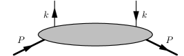
Figure 2: Kinematics for TMDs.

In this subsection we summarize our notation for the TMDs. For the quark sector we follow the conventions of Refs. Mulders and Tangerman (1996); Boer and Mulders (1998); Goeke et al. (2005); Bacchetta et al. (2007), while for the gluons our treatment is similar to Ref. Mulders and Rodrigues (2001), where gluon TMDs were systematically classified for the first time. In Fig. 2 the kinematics for TMDs is indicated. The nucleon momentum is denoted by $P$ (with $P^{2}=M^{2}$), the quark momentum by $k$. The TMDs depend on $k^{+}$, given by the longitudinal momentum fraction

$$x=\frac{k^{+}}{P^{+}}\,,\qquad$$ (44)

and on the transverse momentum $\vec{k}_{T}$. Like in the case of GPDs a possible polarization of the nucleon can conveniently be described by a covariant spin vector $S$, whose components read

$$S^{+}=\frac{\lambda P^{+}}{M}\,,\qquad S^{-}=-\frac{\lambda P^{-}}{M}\,,\qquad\vec{S}_{T}\,.$$ (45)

The quark TMDs are defined through the correlation function

$$\Phi^{q[\Gamma]}(x,\vec{k}_{T};S)$$

$$\ =\frac{1}{2}\int\frac{dz^{-}}{2\pi}\,\frac{d^{2}\vec{z}_{T}}{(2\pi)^{2}}\,e^{ik\cdot z}\,\big{<}P;S\big{|}\,\bar{\psi}\big{(}\!-\!\tfrac{1}{2}z\big{)}\,\Gamma$$

$$\quad\ \,\times\mathcal{W}_{+\infty}\big{(}\!-\!\tfrac{1}{2}z;\tfrac{1}{2}z\big{)}\,\psi\big{(}\tfrac{1}{2}z\big{)}\,\big{|}P;S\big{>}\,\Big{|}_{z^{+}=0^{+}}\,,$$ (46)

in which a summation over the color of the quark fields is implicit, and only connected diagrams have to be considered in perturbative calculations. Like in the case of GPDs, the dependence of the correlator in (II.3) on the renormalization scale is suppressed. The Wilson line in (II.3) is more complicated than the one for the light-cone correlators defining the GPDs Collins and Soper (1982); Collins (2002); Ji and Yuan (2002); Belitsky et al. (2003); Boer et al. (2003a). It can be decomposed according to (see also Fig. 3),

$$\mathcal{W}_{+\infty}\big{(}\!-\!\tfrac{1}{2}z;\tfrac{1}{2}z\big{)}\Big{|}_{z^{+}=0^{+}}$$

$$\ =\big{[}0^{+},-\tfrac{1}{2}z^{-},-\tfrac{1}{2}\vec{z}_{T};0^{+},+\infty^{-},-\tfrac{1}{2}\vec{z}_{T}\big{]}$$

$$\quad\ \,\times\big{[}0^{+},+\infty^{-},-\tfrac{1}{2}\vec{z}_{T};0^{+},+\infty^{-},\tfrac{1}{2}\vec{z}_{T}\big{]}$$

$$\quad\ \,\times\big{[}0^{+},+\infty^{-},\tfrac{1}{2}\vec{z}_{T};0^{+},\tfrac{1}{2}z^{-},\tfrac{1}{2}\vec{z}_{T}\big{]}\,,$$ (47)

where the future-pointing Wilson lines in (II.3) (running along the $z^{-}$ direction in Fig. 3) are appropriate for defining TMDs in SIDIS Collins (2002). In the Drell-Yan process the Wilson lines are necessarily past-pointing Collins (2002), whereas in hadron-hadron scattering with hadronic final states even more complicated paths for the Wilson lines can arise Bomhof et al. (2004); Bacchetta et al. (2005); Bomhof et al. (2006); Bomhof and Mulders (2007). Without loss of generality, in this work just the SIDIS case is considered. If different Wilson lines in (II.3) are used, the results of our model calculations for the TMDs only differ by calculable factors.

Figure 3: Path of Wilson line for TMDs in SIDIS.

In general the use of lightlike Wilson lines in Eq. (II.3) can lead to so-called light-cone divergences Collins and Soper (1982); Collins (2003); Gamberg et al. (2006), and a refined definition of TMDs is needed in order to avoid this problem Collins and Soper (1982); Collins (2003); Ji et al. (2005); Collins and Metz (2004); Hautmann (2007). This issue may make it more difficult to establish model-independent relations between GPDs and TMDs. On the other hand, for the nontrivial relations we are going to study in the context of our low order model calculations no light-cone divergence appears, and the use of the Wilson line in (II.3) is safe.

The leading twist TMDs are obtained from the correlator in (II.3) by using the same three matrices $\Gamma$ as in Eqs. (II.1)–(II.1),

$$\Phi^{q}(x,\vec{k}_{T};S)=\Phi^{q[\gamma^{+}]}(x,\vec{k}_{T};S)$$

$$\ =f_{1}^{q}(x,\vec{k}_{T}^{\,2})-\frac{\epsilon^{ij}_{T}k_{T}^{i}S_{T}^{j}}{M}\,f_{1T}^{\bot q}(x,\vec{k}_{T}^{\,2})\,,$$ (48)

$$\tilde{\Phi}^{q}(x,\vec{k}_{T};S)=\Phi^{q[\gamma^{+}\gamma_{5}]}(x,\vec{k}_{T};S)$$

$$\ =\lambda\,g_{1L}^{q}(x,\vec{k}_{T}^{\,2})+\frac{\vec{k}_{T}\cdot\vec{S}_{T}}{M}\,g_{1T}^{q}(x,\vec{k}_{T}^{\,2})\,,$$ (49)

$$\Phi_{T}^{q,\,j}(x,\vec{k}_{T};S)=\Phi^{q[i\sigma^{j+}\gamma_{5}]}(x,\vec{k}_{T};S)$$

$$\ =-\frac{\epsilon^{ij}_{T}k_{T}^{i}}{M}\,h_{1}^{\bot q}(x,\vec{k}_{T}^{\,2})+\frac{\lambda k_{T}^{j}}{M}\,h_{1L}^{\bot q}(x,\vec{k}_{T}^{\,2})$$

$$\quad\ \,+S_{T}^{j}\,\bigg{(}h_{1T}^{q}(x,\vec{k}_{T}^{\,2})+\frac{\vec{k}_{T}^{\,2}}{2M^{2}}\,h_{1T}^{\bot q}(x,\vec{k}_{T}^{\,2})\bigg{)}$$

$$\quad\ \,+\frac{2k_{T}^{j}\,\vec{k}_{T}\cdot\vec{S}_{T}-S_{T}^{j}\,\vec{k}_{T}^{\,2}}{2M^{2}}\,h_{1T}^{\bot q}(x,\vec{k}_{T}^{\,2})\,.$$ (50)

We note that a number of other notations exist for some of the quark TMDs (see, e.g., Refs. Ralston and Soper (1979); Anselmino et al. (1996); Barone et al. (2002); Idilbi et al. (2004)), and that the corresponding TMDs for antiquarks are again given by the same correlation functions with charge-conjugated fields.

The correlation function for the leading twist gluon TMDs reads

$$\Phi^{g[ij]}(x,\vec{k}_{T};S)$$

$$\ =\frac{1}{xP^{+}}\int\frac{dz^{-}}{2\pi}\,\frac{d^{2}\vec{z}_{T}}{(2\pi)^{2}}\,e^{ik\cdot z}\,\big{<}P;S\big{|}\,F^{+j}_{a}\big{(}\!-\!\tfrac{1}{2}z\big{)}$$

$$\quad\ \,\times\mathcal{W}_{+\infty,ab}\big{(}\!-\!\tfrac{1}{2}z;\tfrac{1}{2}z\big{)}\,F^{+i}_{b}\big{(}\tfrac{1}{2}z\big{)}\,\big{|}P;S\big{>}\,\Big{|}_{z^{+}=0^{+}}\,,$$ (51)

where the path of the Wilson line, now in the adjoint representation, corresponds to Eq. (II.3). It is worthwhile to mention that (II.3) is not the most general gauge invariant operator definition for gluon TMDs. In the most general situation two (different) Wilson lines in the fundamental representation can appear (see also, e.g., Ref. Bomhof and Mulders (2007)), and only in the particular case that these two lines coincide one obtains the definition in Eq. (II.3). However, corresponding to the discussion about more general paths for the Wilson line in the quark correlator (II.3), also for the gluon TMDs a more general Wilson line in (II.3) would merely change the overall factor of our model results and not affect the general conclusions. For simplicity we therefore restrict ourselves to the definition (II.3).

The twist-2 gluon TMDs are now given through the correlator (II.3) according to

$$\Phi^{g}(x,\vec{k}_{T};S)=\delta_{T}^{ij}\,\Phi^{g[ij]}(x,\vec{k}_{T};S)$$

$$\ =f_{1}^{g}(x,\vec{k}_{T}^{\,2})-\frac{\epsilon^{ij}_{T}k_{T}^{i}S_{T}^{j}}{M}\,f_{1T}^{\bot g}(x,\vec{k}_{T}^{\,2})\,,$$ (52)

$$\tilde{\Phi}^{g}(x,\vec{k}_{T};S)=i\epsilon_{T}^{ij}\,\Phi^{g[ij]}(x,\vec{k}_{T};S)$$

$$\ =\lambda\,g_{1L}^{g}(x,\vec{k}_{T}^{\,2})+\frac{\vec{k}_{T}\cdot\vec{S}_{T}}{M}\,g_{1T}^{g}(x,\vec{k}_{T}^{\,2})\,,$$ (53)

$$\Phi_{T}^{g,\,ij}(x,\vec{k}_{T};S)=-\boldsymbol{\hat{S}}\,\Phi^{g[ij]}(x,\vec{k}_{T};S)$$

$$\ =-\frac{\boldsymbol{\hat{S}}\,k_{T}^{i}k_{T}^{j}}{2M^{2}}\,h_{1}^{\bot g}(x,\vec{k}_{T}^{\,2})+\frac{\lambda\,\boldsymbol{\hat{S}}\,k_{T}^{i}\epsilon_{T}^{jk}k_{T}^{k}}{2M^{2}}\,h_{1L}^{\bot g}(x,\vec{k}_{T}^{\,2})$$

$$\quad\ \,+\frac{\boldsymbol{\hat{S}}\,k_{T}^{i}\epsilon_{T}^{jk}S_{T}^{k}}{2M}\,\bigg{(}h_{1T}^{g}(x,\vec{k}_{T}^{\,2})+\frac{\vec{k}_{T}^{\,2}}{2M^{2}}\,h_{1T}^{\bot g}(x,\vec{k}_{T}^{\,2})\bigg{)}$$

$$\quad\ \,+\frac{\boldsymbol{\hat{S}}\,k_{T}^{i}\epsilon_{T}^{jk}\big{(}2k_{T}^{k}\,\vec{k}_{T}\cdot\vec{S}_{T}-S_{T}^{k}\,\vec{k}_{T}^{\,2}\big{)}}{4M^{3}}\,h_{1T}^{\bot g}(x,\vec{k}_{T}^{\,2})\,.$$ (54)

Analogous to the GPD case, the definitions of the chiral-even quark and gluon TMDs correspond to each other [compare the RHS of (II.3) and (II.3), as well as the RHS of (II.3) and (II.3)]. In the chiral-odd sector the definitions of the quark and gluon TMDs are (symbolically) connected by

$$\Phi_{T}^{g,\,ij}\leftrightarrow\boldsymbol{\hat{S}}\,\frac{k_{T}^{i}}{2M}\,\epsilon_{T}^{jk}\Phi_{T}^{q/\bar{q},\,k}$$ (55)

[compare the RHS of (II.3) and (II.3)]. The gluon TMDs defined in Eqs. (II.3)–(II.3) are related to those of Ref. Mulders and Rodrigues (2001) through

$$f_{1}^{g} =+G\,, h_{1}^{\bot g} =+H^{\bot}\,,$$

$$f_{1T}^{\bot g} =-G_{T}\,, h_{1T}^{g} =-\Big{(}\Delta H_{T}-\tfrac{\vec{k}_{T}^{\,2}}{2M^{2}}\Delta H_{T}^{\bot}\Big{)}\,,$$

$$g_{1L}^{g} =-\Delta G_{L}\,, h_{1L}^{\bot g} =-\Delta H_{L}^{\bot}\,,\quad$$

$$g_{1T}^{g} =-\Delta G_{T}\,, h_{1T}^{\bot g} =-\Delta H_{T}^{\bot}\,.$$ (56)

In the forward limit $f_{1}^{g}$ corresponds to the unpolarized gluon distribution, and $g_{1L}^{g}$ coincides with the gluon helicity distribution often denoted by $\Delta G$. Our notation for the gluon TMDs is a natural extension of the nomenclature for quark TMDs. In the context of our work we prefer a notation with small letters for the TMDs in order to avoid confusion with the nomenclature for GPDs. Eventually, notice that yet another notation for gluon TMDs was proposed in Ref. Anselmino et al. (2006a).

Altogether there exist eight leading twist quark TMDs and eight leading twist gluon TMDs, which are all real-valued. Using commutation relations for the parton fields one can derive the symmetry relations

$$Y^{\bar{q}/g}(x,\vec{k}_{T}^{\,2})=\pm\,Y^{q/g}(-x,\vec{k}_{T}^{\,2})$$ (57)

for the TMDs $Y$, where the plus holds for

$$f_{1T}^{\bot q/g},\;g_{1L}^{q/g},\;h_{1}^{\bot q},\;h_{1L}^{\bot q},\;h_{1T}^{g},\;h_{1T}^{\bot g}\,,$$ (58)

and the minus for

$$f_{1}^{q/g},\;g_{1T}^{q/g},\;h_{1}^{\bot g},\;h_{1L}^{\bot g},\;h_{1T}^{q},\;h_{1T}^{\bot q}\,.$$ (59)

Like in the GPD case it is therefore sufficient to consider only the region $x>0$.

The TMDs can also be divided into T-even and T-odd distributions. Whereas on the quark sector two functions are T-odd ($f_{1T}^{\bot q},\;h_{1}^{\bot q}$), there exist four T-odd gluon TMDs ($f_{1T}^{\bot g},\;h_{1L}^{\bot g},\;h_{1T}^{g},\;h_{1T}^{\bot g}$).

The transverse momentum dependent transversity distribution of quarks and gluons is given by

$$h_{1T}^{q/g}(x,\vec{k}_{T}^{\,2})+\frac{\vec{k}_{T}^{\,2}}{2M^{2}}\,h_{1T}^{\bot q/g}(x,\vec{k}_{T}^{\,2})\,.$$ (60)

In the forward limit, where the parton correlators are integrated upon the transverse parton momentum, the gluon transversity drops out. This result is obvious from its prefactor in Eq. (II.3), and ultimately follows from conservation of angular momentum.

With the exception of $f_{1}$ all TMDs characterize the strength of different spin-spin and spin-orbit correlations. The precise form of these correlations is given by the prefactors of the TMDs in Eqs. (II.3)–(II.3) and (II.3)–(II.3). To be more specific, the TMD $g_{1L}$ and the transversity distribution in Eq. (60) describe the strength of a correlation between a longitudinal/transverse target polarization and a longitudinal (circular)/transverse (linear) parton polarization. By definition the spin-orbit correlations invoke the transverse parton momentum and either a polarization of the target ($f_{1T}^{\bot}$), or of the parton ($h_{1}^{\bot}$), or of both ($g_{1T},\;h_{1L}^{\bot},\;h_{1T}^{\bot}$). Note that a corresponding discussion on spin-spin and spin-orbit correlations also applies to the GPDs in impact parameter representation (see, e.g, Ref. Diehl and Hägler (2005)), where the role of the transverse parton momentum in the case of TMDs is played by the impact parameter. In this context the only difference between TMDs and GPDs lies in the fact that the spin-orbit correlations accompanied by the functions $g_{1T}$ and $h_{1L}^{\bot}$ have no counterpart on the GPD side for $\xi=0$ because the corresponding GPDs $\tilde{E}$ and $\tilde{E}_{T}$ do not show up as explained after Eq. (43) (see also the related discussion in Ref. Diehl and Hägler (2005)).

III Relations between GPDs and TMDs: model-independent considerations

In this section the current knowledge on attempts to establish model-independent nontrivial relations between GPDs and TMDs is summarized. As already mentioned earlier, a special role is played by the impact parameter representation of the GPDs, which was used in Ref. Burkardt (2004a) with the aim to find a relation between the GPD $E$ and the Sivers function $f_{1T}^{\perp}$. In Diehl and Hägler (2005) the impact parameter picture was exploited, in particular, to write down (model-independent) analogies between chiral-odd quark GPDs and TMDs. Here the treatment of Ref. Diehl and Hägler (2005) is extended to the gluon sector. It is also argued that it is possible to consider GPDs in momentum instead of impact parameter space if one wants to have some guidance for possible relations between the two types of parton distributions. In addition, we briefly comment on the representation of parton distributions through light-cone wave functions, which also can give some hint on nontrivial relations between GPDs and TMDs.

III.1 Forward parton distributions

For completeness we first recall the well-known trivial relations between GPDs and TMDs. These relations hold due to the connection between GPDs and TMDs on the one hand and ordinary forward parton distributions (PDFs) on the other. For the specific kinematics $\xi=t=0$ some GPDs are related to the three twist-2 PDFs: $f_{1}(x)$ (unpolarized distribution), $g_{1}(x)$ (helicity distribution), and $h_{1}(x)$ (transversity distribution) Ralston and Soper (1979). The same applies to some TMDs if they are integrated upon the transverse parton momentum. To be specific, in our notation one has

$$f_{1}^{q/g}(x)=\int d^{2}\vec{k}_{T}\,f_{1}^{q/g}(x,\vec{k}_{T}^{\,2})$$

$$\ =H^{q/g}(x,0,0)=\int d^{2}\vec{b}_{T}\,\mathcal{H}^{q/g}(x,\vec{b}_{T}^{\,2})\,,$$ (61)

$$g_{1}^{q/g}(x)=\int d^{2}\vec{k}_{T}\,g_{1L}^{q/g}(x,\vec{k}_{T}^{\,2})$$

$$\ =\tilde{H}^{q/g}(x,0,0)=\int d^{2}\vec{b}_{T}\,\mathcal{\tilde{H}}^{q/g}(x,\vec{b}_{T}^{\,2})\,,$$ (62)

$$h_{1}^{q}(x)=\int d^{2}\vec{k}_{T}\,\bigg{(}h_{1T}^{q}(x,\vec{k}_{T}^{\,2})+\frac{\vec{k}_{T}^{\,2}}{2M^{2}}\,h_{1T}^{\bot q}(x,\vec{k}_{T}^{\,2})\bigg{)}$$

$$\ =H_{T}^{q}(x,0,0)\vphantom{\bigg{(}}$$

$$\ =\int d^{2}\vec{b}_{T}\,\bigg{(}\mathcal{H}_{T}^{q}(x,\vec{b}_{T}^{\,2})-\frac{\vec{b}_{T}^{\,2}}{M^{2}}\,\Delta_{b}\mathcal{\tilde{H}}_{T}^{q}(x,\vec{b}_{T}^{\,2})\bigg{)}\,.$$ (63)

Concerning the relations between TMDs and PDFs a word of caution is in order. Already in Sec. II C we mentioned that in general a refined definition for TMDs, containing certain non-lightlike Wilson lines, is needed to avoid possible problems with light-cone divergences. For such a definition the relations between PDFs and TMDs in Eqs. (III.1)–(III.1), in general, turn out to be nontrivial (see, e.g., Refs. Collins (2003); Ji et al. (2005); Hautmann (2007)). However, provided that one avoids the endpoints $x=0$ and $x=1$, for our low order model calculations the definition of TMDs as given in (II.3) and (II.3) does not lead to any problem and all relations (III.1)–(III.1) are satisfied.

III.2 Average transverse momentum

In Ref. Burkardt (2004a) an attempt was made to obtain a nontrivial relation between the GPD $E^{q}$ (in impact parameter representation) and the Sivers function $f_{1T}^{\bot q}$. The object considered there is the average transverse momentum of a quark in a transversely polarized target. The main steps of the treatment of Burkardt (2004a) are repeated here. While in Burkardt (2004a) the light-cone gauge $A^{+}=0$ was used, we do not work in a specific gauge.

The average transverse momentum of an unpolarized quark in a transversely polarized target is defined by

$$\big{<}k_{T}^{q,i}(x)\big{>}_{UT}=\int d^{2}\vec{k}_{T}\,k_{T}^{i}\,\Phi^{q}(x,\vec{k}_{T};S)$$

$$\ =\frac{1}{2}\int d^{2}\vec{k}_{T}\,k_{T}^{i}\,\big{[}\Phi^{q}(x,\vec{k}_{T};\vec{S}_{T})\!-\!\Phi^{q}(x,\vec{k}_{T};-\vec{S}_{T})\big{]}\,,\!\!\!$$ (64)

with the correlator $\Phi^{q}$ in (II.3). The second step on the RHS of (III.2) is justified because obviously only that part of $\Phi^{q}$ which depends on the transverse spin gives rise to a nonvanishing transverse momentum. In the following $\big{<}k_{T}^{q,i}(x)\big{>}_{UT}$ will be expressed in terms of (twist-3) quark-gluon-quark correlation functions Burkardt (2004a); Boer et al. (2003a); Ma and Wang (2004). To do so, we first rewrite the second term on the RHS of (III.2) by means of the parity and time-reversal transformation,

$$\Phi^{q}(x,\vec{k}_{T};-\vec{S}_{T})$$

$$\ =\frac{1}{2}\int\frac{dz^{-}}{2\pi}\,\frac{d^{2}\vec{z}_{T}}{(2\pi)^{2}}\,e^{ik\cdot z}\,\big{<}P;-\vec{S}_{T}\big{|}\,\bar{\psi}\big{(}\!-\!\tfrac{1}{2}z\big{)}\,\gamma^{+}$$

$$\quad\ \,\times\mathcal{W}_{+\infty}\big{(}\!-\!\tfrac{1}{2}z;\tfrac{1}{2}z\big{)}\,\psi\big{(}\tfrac{1}{2}z\big{)}\,\big{|}P;-\vec{S}_{T}\big{>}\,\Big{|}_{z^{+}=0^{+}}$$

$$\ =\frac{1}{2}\int\frac{dz^{-}}{2\pi}\,\frac{d^{2}\vec{z}_{T}}{(2\pi)^{2}}\,e^{ik\cdot z}\,\big{<}P;\vec{S}_{T}\big{|}\,\bar{\psi}\big{(}\!-\!\tfrac{1}{2}z\big{)}\,\gamma^{+}$$

$$\quad\ \,\times\mathcal{W}_{-\infty}\big{(}\!-\!\tfrac{1}{2}z;\tfrac{1}{2}z\big{)}\,\psi\big{(}\tfrac{1}{2}z\big{)}\,\big{|}P;\vec{S}_{T}\big{>}\,\Big{|}_{z^{+}=0^{+}}\,.$$ (65)

This leads to the intermediate result

$$\big{<}k_{T}^{q,i}(x)\big{>}_{UT}$$

$$\ =\frac{1}{4}\int d^{2}\vec{k}_{T}\,k_{T}^{i}\,\int\frac{dz^{-}}{2\pi}\,\frac{d^{2}\vec{z}_{T}}{(2\pi)^{2}}\,e^{ik\cdot z}\,\big{<}P;\vec{S}_{T}\big{|}\,\bar{\psi}\big{(}\!-\!\tfrac{1}{2}z\big{)}\,\gamma^{+}$$

$$\quad\ \,\times\,\Big{[}\mathcal{W}_{+\infty}\big{(}\!-\!\tfrac{1}{2}z;\tfrac{1}{2}z\big{)}-\mathcal{W}_{-\infty}\big{(}\!-\!\tfrac{1}{2}z;\tfrac{1}{2}z\big{)}\Big{]}$$

$$\quad\ \,\times\psi\big{(}\tfrac{1}{2}z\big{)}\,\big{|}P;\vec{S}_{T}\big{>}\,\Big{|}_{z^{+}=0^{+}}$$

$$\ =\frac{i}{4}\int\frac{dz^{-}}{2\pi}\,e^{ik\cdot z}\,\partial_{T}^{i}\,\big{<}P;\vec{S}_{T}\big{|}\,\bar{\psi}\big{(}\!-\!\tfrac{1}{2}z\big{)}\,\gamma^{+}$$

$$\quad\ \,\times\,\Big{[}\mathcal{W}_{+\infty}\big{(}\!-\!\tfrac{1}{2}z;\tfrac{1}{2}z\big{)}-\mathcal{W}_{-\infty}\big{(}\!-\!\tfrac{1}{2}z;\tfrac{1}{2}z\big{)}\Big{]}$$

$$\quad\ \,\times\psi\big{(}\tfrac{1}{2}z\big{)}\,\big{|}P;\vec{S}_{T}\big{>}\,\Big{|}\,\!_{\begin{subarray}{c}z^{+}=0^{+}\\ \vec{z}_{T}=\vec{0}_{T}\end{subarray}}\,.$$ (66)

In order to perform the second step in (III.2) we have expressed the factor $k_{T}^{i}$ through the transverse derivative $\partial_{T}^{i}$ acting on the exponential, and performed an integration by parts.

The derivative in (III.2) can now act either on the quark fields or on the Wilson lines. In the first case though, one gets no contribution to the average transverse momentum, since the involved combination of Wilson lines vanishes,

$$\Big{[}\mathcal{W}_{+\infty}\big{(}\!-\!\tfrac{1}{2}z;\tfrac{1}{2}z\big{)}-\mathcal{W}_{-\infty}\big{(}\!-\!\tfrac{1}{2}z;\tfrac{1}{2}z\big{)}\Big{]}\,\Big{|}\,\!_{\begin{subarray}{c}z^{+}=0^{+}\\ \vec{z}_{T}=\vec{0}_{T}\end{subarray}}=0\,.$$ (67)

The result (67) is obvious because both Wilson lines are just running along the light-cone.

On the other hand, if the derivative acts on the Wilson lines, one finds

$$i\,\partial_{T}^{i}\,\Big{[}\mathcal{W}_{+\infty}\big{(}\!-\!\tfrac{1}{2}z;\tfrac{1}{2}z\big{)}-\mathcal{W}_{-\infty}\big{(}\!-\!\tfrac{1}{2}z;\tfrac{1}{2}z\big{)}\Big{]}\,\Big{|}\,\!_{\begin{subarray}{c}z^{+}=0^{+}\\ \vec{z}_{T}=\vec{0}_{T}\end{subarray}}$$

$$\ =g\int dy^{-}\,\mathcal{W}\big{(}\!-\!\tfrac{1}{2}z;y\big{)}\,t_{a}\,F^{+i}_{a}\big{(}y\big{)}\mathcal{W}\big{(}y;\tfrac{1}{2}z\big{)}\,\Big{|}\,\!_{\begin{subarray}{c}y^{+}=z^{+}=0^{+}\\ \vec{y}_{T}=\vec{z}_{T}=\vec{0}_{T}\end{subarray}}$$

$$\ =2\,\mathcal{W}\big{(}\!-\!\tfrac{1}{2}z;\tfrac{1}{2}z\big{)}\,I^{q,i}\big{(}\tfrac{1}{2}z\big{)}\,\Big{|}\,\!_{\begin{subarray}{c}z^{+}=0^{+}\\ \vec{z}_{T}=\vec{0}_{T}\end{subarray}}\,,$$ (68)

where the paths of the remaining Wilson lines run along the light-cone and the function $I^{q,i}$ is defined by

$$I^{q,i}\big{(}\tfrac{1}{2}z\big{)}$$

$$=\frac{g}{2}\int dy^{-}\,\mathcal{W}\big{(}\tfrac{1}{2}z;y\big{)}\,t_{a}\,F^{+i}_{a}\big{(}y\big{)}\,\mathcal{W}\big{(}y;\tfrac{1}{2}z\big{)}\,\Big{|}\,\!_{\begin{subarray}{l}y^{+}=z^{+}\\ \vec{y}_{T}=\vec{z}_{T}\end{subarray}}\,.$$ (69)

Plugging the results together one arrives at the following expression for the average transverse momentum,

$$\big{<}k_{T}^{q,i}(x)\big{>}_{UT}$$

$$\ =\frac{1}{2}\int\frac{dz^{-}}{2\pi}\,e^{ik\cdot z}\,\big{<}P;\vec{S}_{T}\big{|}\,\bar{\psi}\big{(}\!-\!\tfrac{1}{2}z\big{)}\,\gamma^{+}$$

$$\quad\ \,\times\mathcal{W}\big{(}\!-\!\tfrac{1}{2}z;\tfrac{1}{2}z\big{)}\,I^{q,i}\big{(}\tfrac{1}{2}z\big{)}\,\psi\big{(}\tfrac{1}{2}z\big{)}\,\big{|}P;\vec{S}_{T}\big{>}\,\Big{|}\,\!_{\begin{subarray}{c}z^{+}=0^{+}\\ \vec{z}_{T}=\vec{0}_{T}\end{subarray}}\,.\!\!\!\!$$ (70)

Equation (III.2) is a representation of the average transverse momentum in terms of a specific quark-gluon-quark light-cone correlator Burkardt (2004a); Boer et al. (2003a); Ma and Wang (2004). Since the gluon field in the three-parton correlator in (III.2) has zero longitudinal momentum one often talks about a soft gluon matrix element. The reader is referred to Efremov and Teryaev (1982, 1985); Qiu and Sterman (1991, 1992) where such (or similar) matrix elements were first discussed in connection with transverse SSAs.

To unravel a possible connection between the Sivers effect and the GPD $E^{q}$, in Ref. Burkardt (2004a) the RHS of (III.2) was transformed to the impact parameter space, where it takes the form

$$\big{<}k_{T}^{q,i}(x)\big{>}_{UT}$$

$$\ =\frac{1}{2}\int d^{2}\vec{b}_{T}\,\int\frac{dz^{-}}{2\pi}\,e^{ixP^{+}z^{-}}\,\big{<}P^{+},\vec{0}_{T};S\big{|}\,\bar{\psi}\big{(}z_{1}\big{)}\,\gamma^{+}$$

$$\quad\ \,\times\mathcal{W}\big{(}z_{1};z_{2}\big{)}\,I^{q,i}\big{(}z_{2}\big{)}\,\psi\big{(}z_{2}\big{)}\,\big{|}P^{+},\vec{0}_{T};S\big{>}\,,$$ (71)

with $z_{1/2}$ as given in Eq. (36). Comparing the expression in (III.2) with the correlator (II.2) for the quark GPDs in impact parameter space (for $\Gamma=\gamma^{+}$) one realizes that the only difference is the additional factor $I^{q,i}$ and an integration upon the impact parameter $\vec{b}_{T}$ Burkardt (2004a). On the basis of this observation one may hope to find a relation of the type

$$\big{<}k_{T}^{q,i}(x)\big{>}_{UT}=\int d^{2}\vec{k}_{T}\,k_{T}^{i}\,\Phi^{q}(x,\vec{k}_{T};S)$$

$$\ \simeq\int d^{2}\vec{b}_{T}\,\mathcal{I}^{q,i}(x,\vec{b}_{T})\,\mathcal{F}^{q}(x,\vec{b}_{T};S)\,,$$ (72)

where, in rough terms, the function $\mathcal{I}^{q,i}$ incorporates the effect of the gluon field in the correlator on the RHS of (III.2). We mention that in the second term on the RHS of (III.2) only the spin-dependent term of ${\mathcal{F}}^{q}$ contributes.

Expressed in terms of TMDs and GPDs Eq. (III.2) reads

$$\big{<}k_{T}^{q,i}(x)\big{>}_{UT}$$

$$\ =-\int d^{2}\vec{k}_{T}\,k_{T}^{i}\,\frac{\epsilon_{T}^{jk}k_{T}^{j}S_{T}^{k}}{M}\,f_{1T}^{\bot q}(x,\vec{k}_{T}^{\,2})$$

$$\ \simeq\int d^{2}\vec{b}_{T}\,\mathcal{I}^{q,i}(x,\vec{b}_{T})\,\frac{\epsilon_{T}^{jk}b_{T}^{j}S_{T}^{k}}{M}\,\bigg{(}\mathcal{E}^{q}(x,\vec{b}_{T}^{\,2})\bigg{)}^{\prime}\,.$$ (73)

Interestingly, the relation (III.2) is indeed fulfilled in the context of perturbative low order model calculations Burkardt and Hwang (2004) (see also Sec. IV). It also provides an intuitive understanding of the origin of the Sivers transverse SSA Burkardt (2002, 2004a). However, Eq. (III.2) does not have the status of a general, model-independent result (see also, e.g., Ref. Burkardt (2007)). The crucial problem lies in the fact that, in general, the average transverse momentum $\big{<}k_{T}^{q,i}(x)\big{>}_{UT}$ caused by the Sivers effect cannot be factorized into the function $\mathcal{I}^{q,i}$ (called lensing function in Burkardt (2004a)) and the distortion of the impact parameter distribution of quarks in a transversely polarized target which is determined by $(\mathcal{E}^{q})^{\prime}$.

III.3 Generalization of relations

To get further insight into possible relations between GPDs and TMDs, which at least may hold in the context of model calculations, we now follow a procedure given in Ref. Diehl and Hägler (2005). The equations defining the GPDs in impact parameter space [see Eqs. (II.2)–(II.2)] on the one hand and the TMDs [see Eqs. (II.3)–(II.3) and (II.3)–(II.3)] on the other obviously have a corresponding structure if one interchanges the impact parameter $\vec{b}_{T}$ and the transverse momentum $\vec{k}_{T}$. Comparing these equations one directly finds out which functions may be related. However, using this procedure one cannot extract the precise form of the relations. Note also that the two TMDs $g_{1T}$ and $h_{1L}^{\bot}$ have no counterpart on the GPD side, as already pointed out in Sec. II C. In the following we, respectively, talk about relations of first, second, third, and fourth type, depending on the number of derivatives of the involved GPDs in impact parameter space. In the case of quark distributions the results given in this subsection were already presented in Ref. Diehl and Hägler (2005). At this point one has to keep in mind that, apart from the trivial model-independent relations (relations of first type), all relations presented in this and the following subsection so far have only the status of analogies between functions which follow from obvious analogies in the structures of the GPD and TMD correlators. Quantitative relations will be discussed in Sec. IV in connection with model calculations.

First of all, one finds the following connections by means of the mentioned comparison,

$$f_{1}^{q/g}\leftrightarrow\mathcal{H}^{q/g}\,, \qquad g_{1L}^{q/g}\leftrightarrow\mathcal{\tilde{H}}^{q/g}\,,$$

$$\Big{(}h_{1T}^{q}+\tfrac{\vec{k}_{T}^{\,2}}{2M^{2}}\,h_{1T}^{\bot q}\Big{)} \leftrightarrow\Big{(}\mathcal{H}_{T}^{q}-\tfrac{\vec{b}_{T}^{\,2}}{M^{2}}\,\Delta_{b}\mathcal{\tilde{H}}_{T}^{q}\Big{)}\,,$$ (74)

which simply correspond to the trivial relations discussed in Sec. III A.

Relations of second type contain GPDs with one derivative,

$$f_{1T}^{\bot q/g}\leftrightarrow-\Big{(}\mathcal{E}^{q/g}\Big{)}^{\prime}\,, \qquad h_{1}^{\bot q}\leftrightarrow-\Big{(}\mathcal{E}_{T}^{q}+2\mathcal{\tilde{H}}_{T}^{q}\Big{)}^{\prime}\,,$$

$$\Big{(}h_{1T}^{g}+\tfrac{\vec{k}_{T}^{\,2}}{2M^{2}}\,h_{1T}^{\bot g}\Big{)} \leftrightarrow-2\Big{(}\mathcal{H}_{T}^{g}-\tfrac{\vec{b}_{T}^{\,2}}{M^{2}}\,\Delta_{b}\mathcal{\tilde{H}}_{T}^{g}\Big{)}^{\prime}\,,$$ (75)

where the first relation in (III.3) involving $f_{1T}^{\bot q}$ and the derivative of $\mathcal{E}^{q}$ corresponds to Eq. (III.2). At this point it is also worthwhile to notice that the computation of the average transverse momentum of a transversely polarized quark in an unpolarized target, using the correlator in Eq. (II.3), can be carried out completely analogous to Sec. III B above where the transverse momentum caused by the Sivers effect is considered. Doing so, one eventually obtains an equation corresponding to (III.2), with the quark Boer-Mulders function $h_{1}^{\bot q}$ showing up on the TMD side, and the first derivative of the linear combination $\mathcal{E}_{T}^{q}+2\mathcal{\tilde{H}}_{T}^{q}$ on the GPD side. On the basis of these considerations one, in particular, also expects the same lensing function $\mathcal{I}^{q,i}$ to appear in the analogue of Eq. (III.2). This feature indeed emerges in the context of the model calculations presented in Sec. IV. We note that a corresponding discussion also holds for both relations between gluon GPDs and TMDs in Eq. (III.3).

Finally, one obtains two relations of third type, containing GPDs with a second derivative,

$$h_{1T}^{\bot q}\leftrightarrow 2\Big{(}\mathcal{\tilde{H}}_{T}^{q}\Big{)}^{\prime\prime}\,,\qquad h_{1}^{\bot g}\leftrightarrow 2\Big{(}\mathcal{E}_{T}^{g}+2\mathcal{\tilde{H}}_{T}^{g}\Big{)}^{\prime\prime}\,,$$ (76)

and on the gluon sector even one relation where a GPD enters with its third derivative,

$$h_{1T}^{\bot g}\leftrightarrow-4\Big{(}\mathcal{\tilde{H}}_{T}^{g}\Big{)}^{\prime\prime\prime}\,.$$ (77)

We emphasize that the number of derivatives of the GPDs in the various relations in a first place merely distinguishes between the different type of relations, even though in specific model calculations one may find relations with exactly the number of derivatives showing up in (III.3)–(77). For the relations of first, second, and third type in Eqs. (III.3)–(76) this works, e.g., in the context of simple spectator models as outlined in Sec. IV below. We cannot check this feature for the relation of fourth type (77) by our model calculations because the respective parton distributions vanish.

III.4 Relations in momentum space

The relations presented in the previous subsection were obtained by comparing the equations defining the GPDs in the impact parameter representation (for $\xi=0$) with those defining the TMDs. Here we argue that there is actually no need to make the Fourier transform to the impact parameter space. Relations corresponding to (III.3)–(77) also emerge if one compares Eqs. (II.3)–(II.3) and (II.3)–(II.3) on the TMD side with the momentum space correlators for GPDs in (II.1)–(II.1) and (II.1)–(II.1) evaluated at $\xi=0$.

At the particular kinematical point $\xi=0$ the RHS of Eqs. (II.1)–(II.1) and (II.1)–(II.1) can be simplified considerably. Using the spin vector $S$ introduced in Sec. II B one finds after straightforward algebra

$$F^{q/g}(x,\Delta_{T};S)$$

$$\ =H^{q/g}(x,0,\!-\vec{\Delta}_{T}^{2})-\frac{i\epsilon^{ij}_{T}\Delta_{T}^{i}S_{T}^{j}}{2M}\,E^{q/g}(x,0,\!-\vec{\Delta}_{T}^{2})\,,\!\!\!\!\!$$ (78)

$$\tilde{F}^{q/g}(x,\Delta_{T};S)$$

$$\ =\lambda\,\tilde{H}^{q/g}(x,0,-\vec{\Delta}_{T}^{2})\,,$$ (79)

$$F_{T}^{q,\,j}(x,\Delta_{T};S)$$

$$\ =-\frac{i\epsilon^{ij}_{T}\Delta_{T}^{i}}{2M}\,\bigg{(}E_{T}^{q}(x,0,-\vec{\Delta}_{T}^{2})+2\tilde{H}_{T}^{q}(x,0,-\vec{\Delta}_{T}^{2})\bigg{)}$$

$$\quad\ \,+S_{T}^{j}\,\bigg{(}H_{T}^{q}(x,0,-\vec{\Delta}_{T}^{2})+\frac{\vec{\Delta}_{T}^{2}}{4M^{2}}\,\tilde{H}_{T}^{q}(x,0,-\vec{\Delta}_{T}^{2})\bigg{)}$$

$$\quad\ \,-\frac{2\Delta_{T}^{j}\,\vec{\Delta}_{T}\cdot\vec{S}_{T}-S_{T}^{j}\,\vec{\Delta}_{T}^{2}}{4M^{2}}\,\tilde{H}_{T}^{q}(x,0,-\vec{\Delta}_{T}^{2})\,,$$ (80)

$$F_{T}^{g,\,ij}(x,\Delta_{T};S)$$

$$\ =\frac{\boldsymbol{\hat{S}}\,\Delta_{T}^{i}\Delta_{T}^{j}}{4M^{2}}\,\bigg{(}E_{T}^{g}(x,0,-\vec{\Delta}_{T}^{2})+2\tilde{H}_{T}^{g}(x,0,-\vec{\Delta}_{T}^{2})\bigg{)}$$

$$\quad\ \,+\frac{i\boldsymbol{\hat{S}}\,\Delta_{T}^{i}\epsilon_{T}^{jk}S_{T}^{k}}{2M}\,\bigg{(}H_{T}^{g}(x,0,-\vec{\Delta}_{T}^{2})$$

$$\qquad\qquad+\frac{\vec{\Delta}_{T}^{2}}{4M^{2}}\,\tilde{H}_{T}^{g}(x,0,-\vec{\Delta}_{T}^{2})\bigg{)}$$

$$\quad\ \,-\frac{i\boldsymbol{\hat{S}}\,\Delta_{T}^{i}\epsilon_{T}^{jk}\big{(}2\Delta_{T}^{k}\,\vec{\Delta}_{T}\cdot\vec{S}_{T}-S_{T}^{k}\,\vec{\Delta}_{T}^{2}\big{)}}{8M^{3}}$$

$$\qquad\qquad\times\tilde{H}_{T}^{g}(x,0,-\vec{\Delta}_{T}^{2})\,.$$ (81)

We repeat that the GPDs $\tilde{E}$ and $\tilde{E}_{T}$ do not show up in the expressions above because of the choice $\xi=0$.

One readily observes that the structure of Eqs. (III.4)–(III.4) corresponds to the structure of (II.3)–(II.3) and (II.3)–(II.3). To be more specific, if one replaces $-i\vec{\Delta}_{T}/2$ in the prefactors of the former equations by the transverse momentum $\vec{k}_{T}$ one recovers the various prefactors of the latter. This strong similarity of the correlators for GPDs (in momentum space) and TMDs also allows one, like in Sec. III C, to write down relations between the two types of parton distributions. In the following we refer again to relations of first, second, third, and fourth type, where the relations of first type are given by

$$f_{1}^{q/g}\leftrightarrow H^{q/g}\,, \qquad g_{1L}^{q/g}\leftrightarrow{\tilde{H}}^{q/g}\,,$$

$$\Big{(}h_{1T}^{q}+\tfrac{\vec{k}_{T}^{\,2}}{2M^{2}}\,h_{1T}^{\bot q}\Big{)} \leftrightarrow\Big{(}H_{T}^{q}+\tfrac{\vec{\Delta}_{T}^{2}}{4M^{2}}\,{\tilde{H}}_{T}^{q}\Big{)}\,.$$ (82)

The relations of second type read

$$f_{1T}^{\bot q/g}\leftrightarrow-\Big{(}E^{q/g}\Big{)}\,, \qquad h_{1}^{\bot q}\leftrightarrow-\Big{(}E_{T}^{q}+2{\tilde{H}}_{T}^{q}\Big{)}\,,$$

$$\Big{(}h_{1T}^{g}+\tfrac{\vec{k}_{T}^{\,2}}{2M^{2}}\,h_{1T}^{\bot g}\Big{)} \leftrightarrow-2\Big{(}H_{T}^{g}+\tfrac{\vec{\Delta}_{T}^{2}}{4M^{2}}\,{\tilde{H}}_{T}^{g}\Big{)}\,,$$ (83)

and one finds

$$h_{1T}^{\bot q}\leftrightarrow 2\Big{(}{\tilde{H}}_{T}^{q}\Big{)}\,,\qquad h_{1}^{\bot g}\leftrightarrow 2\Big{(}E_{T}^{g}+2{\tilde{H}}_{T}^{g}\Big{)}\,,$$ (84)

for the relations of third type, as well as

$$h_{1T}^{\bot g}\leftrightarrow-4\Big{(}{\tilde{H}}_{T}^{g}\Big{)}\,.$$ (85)

for the one relation of fourth type. One may wonder why we distinguish here between different types of relations. The reason is simply that, in the defining equations, the prefactors of the GPDs and TMDs carry different powers of $\vec{\Delta}_{T}$ and $\vec{b}_{T}$, respectively. If there appears no $\vec{\Delta}_{T}$ or $\vec{b}_{T}$ in the prefactor we talk about a relation of first type, if they appear linearly we talk about a relation of second type and so on. In connection with this discussion it may be worthwhile to mention that the number of derivatives of the GPDs in impact parameter representation matches with the power of $\vec{\Delta}_{T}$ in the corresponding prefactors in Eqs. (III.4)–(III.4). This correspondence just reflects a property of the Fourier transform from the momentum space to the impact parameter space.

Observe now the close analogy between the relations in (III.4)–(85) and those in (III.3)–(77). In the context of our model calculations in Sec. IV we will consider relations between TMDs and GPDs in both impact parameter space as well as momentum space.

Eventually, let us briefly comment on nontrivial relations between GPDs and TMDs that can be obtained by looking at a light-cone wave function representation of these objects. This issue was, in particular, discussed in connection with a possible relation between the quark Sivers function and the GPD $E^{q}$ (see, e.g., Refs. Brodsky et al. (2002a); Brodsky and Gardner (2006); Brodsky and Yuan (2006); Lu and Schmidt (2007)). One finds that for both parton distributions the same light-cone wave functions appear, which hints at a close relation between $f_{1T}^{\bot q}$ and $E^{q}$. However, it turns out that in the case of the Sivers function one has to augment the involved wave functions by a phase factor not present in the case of $E^{q}$ Brodsky and Gardner (2006). This phase spoils a model-independent one-to-one correspondence between $f_{1T}^{\bot}$ and $E^{q}$. So far only in the context of simple models the Sivers function can be represented through real wave functions multiplied by some additional factor Brodsky et al. (2002a); Lu and Schmidt (2007), allowing one to establish a direct connection between the two distributions.

Moreover, in general (in full QCD) the representation of parton distributions in terms of light-cone wave functions may be problematic. This feature was already observed in the case of the unpolarized parton distribution $f_{1}^{q}(x)$ in Ref. Brodsky et al. (2002b).

IV Relations between GPDs and TMDs: results of model calculations

While the previous Sec. III is devoted to model-independent considerations on possible relations between GPDs and TMDs, here we discuss the relations in the context of specific model results. To do so, two spectator models are studied: first, the scalar diquark spectator model of the nucleon (see, e.g., Ref. Brodsky et al. (2002a)); second, a quark target model treated in perturbative QCD. Some details concerning these models as well as the full list of GPDs and TMDs, computed to lowest nontrivial order in perturbation theory, can be found in the appendices.

IV.1 Relations of first type

We start this discussion with the relations of first type in Eqs. (III.1)–(III.1). As an example consider the TMD $f_{1}^{q}$ in (122) and the GPD $H^{q}$ in (133) in the scalar diquark model. Using these results one readily verifies that

$$f_{1}^{q}(x)=\int d^{2}\vec{k}_{T}\,f_{1}^{q}(x,\vec{k}_{T}^{\,2})$$

$$\ =\frac{g^{2}(1-x)}{2(2\pi)^{3}}\,\int d^{2}\vec{k}_{T}\,\frac{\vec{k}_{T}^{\,2}+(m_{q}+xM)^{2}}{\big{[}\vec{k}_{T}^{\,2}+\tilde{M}^{2}(x)\big{]}\,\!^{2}}$$

$$\ =H^{q}(x,0,0)=\int d^{2}\vec{b}_{T}\,\mathcal{H}^{q}(x,\vec{b}_{T}^{\,2})\,,$$ (86)

i.e., that the relation (III.1) holds. The unpolarized distributions of scalar diquarks and of quarks and gluons in the quark target model satisfy Eq. (III.1) as well. Moreover, the results in both models obey the relations (III.1) and (III.1). Of course the model results have to satisfy these model-independent relations. Therefore, the comparison discussed here merely serves as a consistency check of the calculation.

IV.2 Relations of second type

In order to study the relations of second type in Eq. (III.3) in the context of our model calculations we first consider the average transverse momentum of a parton caused by the Sivers effect (see Sec. III B). Details of the calculation are given for a quark in the scalar spectator model. It turns out that the transverse momentum can indeed be expressed according to Eq. (III.2) in terms of $(\mathcal{E}^{q})^{\prime}$. The reader is referred to Burkardt and Hwang (2004) where the connection in (III.2) in the context of the spectator model was presented for the first time.

By definition the average transverse momentum of an unpolarized quark in a transversely polarized target is given by [see also (III.2)]

$$\big{<}k_{T}^{q,i}(x)\big{>}_{UT}$$

$$\ =-\int d^{2}\vec{k}_{T}\,k_{T}^{i}\,\frac{\epsilon_{T}^{jk}k_{T}^{j}S_{T}^{k}}{M}\,f_{1T}^{\bot q}(x,\vec{k}_{T}^{\,2})$$

$$\ =-\frac{g^{2}e_{q}e_{s}(1-x)(m_{q}+xM)}{4(2\pi)^{4}}\,\int d^{2}\vec{k}_{T}$$

$$\quad\ \,\times\frac{k_{T}^{i}\,\epsilon_{T}^{jk}k_{T}^{j}S_{T}^{k}}{\vec{k}_{T}^{\,2}\,\big{[}\vec{k}_{T}^{\,2}+\tilde{M}^{2}(x)\big{]}}\,\ln\bigg{(}\frac{\vec{k}_{T}^{\,2}+\tilde{M}^{2}(x)}{\tilde{M}^{2}(x)}\bigg{)}$$

$$\ =\frac{g^{2}e_{q}e_{s}(1-x)(m_{q}+xM)}{2(2\pi)^{3}}\,\int\frac{d^{2}\vec{l}_{T}}{(2\pi)^{2}}\,\frac{l_{T}^{i}}{\vec{l}_{T}^{\,2}}\,\int d^{2}\vec{k}_{T}$$

$$\quad\ \,\times\frac{\epsilon_{T}^{jk}k_{T}^{j}S_{T}^{k}}{\big{[}\vec{k}_{T}^{\,2}+\tilde{M}^{2}(x)\big{]}\,\big{[}\big{(}\vec{k}_{T}+\vec{l}_{T}\big{)}\,\!^{2}+\tilde{M}^{2}(x)\big{]}}\,,$$ (87)

where we have inserted the result for the Sivers function from Eq. (123) and used in the last step that

$$\int\frac{d^{2}\vec{l}_{T}}{(2\pi)^{2}}\,\frac{l_{T}^{i}}{\vec{l}_{T}^{\,2}\,\big{[}\big{(}\vec{k}_{T}+\vec{l}_{T}\big{)}\,\!^{2}+\tilde{M}^{2}(x)\big{]}}$$

$$\ =-\frac{k_{T}^{i}}{4\pi\,\vec{k}_{T}^{\,2}}\,\ln\bigg{(}\frac{\vec{k}_{T}^{\,2}+\tilde{M}^{2}(x)}{\tilde{M}^{2}(x)}\bigg{)}\,.$$ (88)

If one now replaces the integration variable $\vec{k}_{T}$ according to $\vec{k}_{T}\rightarrow-\vec{k}_{T}-\vec{l}_{T}$ one gets

$$\!\!\big{<}k_{T}^{q,i}(x)\big{>}_{UT}$$

$$\!\!\ =-\frac{g^{2}e_{q}e_{s}(1-x)(m_{q}+xM)}{4(2\pi)^{3}}\,\int\frac{d^{2}\vec{l}_{T}}{(2\pi)^{2}}\,\frac{l_{T}^{i}}{\vec{l}_{T}^{\,2}}\,\int d^{2}\vec{k}_{T}$$

$$\!\!\quad\ \,\times\frac{\epsilon_{T}^{jk}l_{T}^{j}S_{T}^{k}}{\big{[}\vec{k}_{T}^{\,2}+\tilde{M}^{2}(x)\big{]}\,\big{[}\big{(}\vec{k}_{T}+\vec{l}_{T}\big{)}\,\!^{2}+\tilde{M}^{2}(x)\big{]}}$$

$$\!\!\ =-\frac{e_{q}e_{s}}{4}\int\!\frac{d^{2}\vec{l}_{T}}{(2\pi)^{2}}\,\frac{l_{T}^{i}}{\vec{l}_{T}^{\,2}}\,\frac{\epsilon_{T}^{jk}l_{T}^{j}S_{T}^{k}}{(1-x)M}\,E^{q}\Big{(}x,0,\!-\tfrac{\vec{l}_{T}^{\,2}}{(1-x)^{2}}\Big{)}\,,\!\!$$ (89)

where we took for $E^{q}$ the result in Eq. (134). In the next step the transformation to the impact parameter space is performed which leads to

$$\big{<}k_{T}^{q,i}(x)\big{>}_{UT}$$

$$\ =-\frac{e_{q}e_{s}}{4}\,\int\frac{d^{2}\vec{l}_{T}}{(2\pi)^{2}}\,\frac{l_{T}^{i}}{\vec{l}_{T}^{\,2}}$$

$$\quad\ \,\times\frac{\epsilon_{T}^{jk}l_{T}^{j}S_{T}^{k}}{(1-x)M}\,\int d^{2}\vec{b}_{T}\,e^{i\tfrac{\vec{l}_{T}\cdot\vec{b}_{T}}{1-x}}\,\mathcal{E}^{q}(x,\vec{b}_{T}^{\,2})$$

$$\ =\int d^{2}\vec{b}_{T}\,\frac{ie_{q}e_{s}}{2}\,\int\frac{d^{2}\vec{l}_{T}}{(2\pi)^{2}}\,e^{-i\tfrac{\vec{l}_{T}\cdot\vec{b}_{T}}{1-x}}\,\frac{l_{T}^{i}}{\vec{l}_{T}^{\,2}}$$

$$\quad\ \,\times\frac{\epsilon_{T}^{jk}b_{T}^{j}S_{T}^{k}}{M}\,\bigg{(}\mathcal{E}^{q}(x,\vec{b}_{T}^{\,2})\bigg{)}^{\prime}$$

$$\ =\int d^{2}\vec{b}_{T}\,\mathcal{I}_{\textrm{SDM}}^{q,i}(x,\vec{b}_{T})\,\frac{\epsilon_{T}^{jk}b_{T}^{j}S_{T}^{k}}{M}\,\bigg{(}\mathcal{E}^{q}(x,\vec{b}_{T}^{\,2})\bigg{)}^{\prime}\,.$$ (90)

In (IV.2) integration by parts is used in order to obtain a representation of the transverse quark momentum that contains the derivative of ${\mathcal{E}}^{q}$. Equation (IV.2) coincides with the relation in (III.2) between the Sivers function and the GPD $E^{q}$, where the so-called lensing function Burkardt (2004a) $\mathcal{I}_{\textrm{SDM}}^{q,i}$ is given by

$$\mathcal{I}_{\textrm{SDM}}^{q,i}(x,\vec{b}_{T})=\frac{ie_{q}e_{s}}{2}\,\int\frac{d^{2}\vec{l}_{T}}{(2\pi)^{2}}\,e^{-i\tfrac{\vec{l}_{T}\cdot\vec{b}_{T}}{1-x}}\,\frac{l_{T}^{i}}{\vec{l}_{T}^{\,2}}$$

$$\ =\frac{e_{q}e_{s}}{4\pi}\frac{(1-x)\,b_{T}^{i}}{\vec{b}_{T}^{\,2}}\,.$$ (91)

The calculation in (IV.2)–(IV.2) also goes through step by step if one considers the average transverse momentum of diquarks in the diquark spectator model, using the Sivers function $f_{1T}^{\bot s}$ from (131) and the GPD $E^{s}$ from (140). One finds that the lensing functions for quarks and diquarks in that model are the same,

$$\mathcal{I}_{\textrm{SDM}}^{s,i}(x,\vec{b}_{T})=\mathcal{I}_{\textrm{SDM}}^{q,i}(x,\vec{b}_{T})\,.$$ (92)

Moreover, the transverse momentum $\big{<}k_{T}^{i}(x)\big{>}_{UT}$ can also be computed for quarks and gluons in the quark target model. On the basis of the respective results given in Appendix B one obtains in that case the lensing functions

$$\mathcal{I}_{\textrm{QTM}}^{q,i}(x,\vec{b}_{T})=\mathcal{I}_{\textrm{QTM}}^{g,i}(x,\vec{b}_{T})=-\frac{3g^{2}}{8\pi}\frac{(1-x)\,b_{T}^{i}}{\vec{b}_{T}^{\,2}}\,.$$ (93)

Therefore, all results in the two spectator models satisfy the relation between the Sivers function and the GPD $E$ in (III.3), where the specific form of the relation is given in Eq. (III.2). In the context of the model calculations the lensing function does not depend on the parton type but merely on the model, which means in other words that it just depends on the target. Note that in both models the lensing function has the same overall sign and is negative.

At this point we would like to add some discussion on the intuitive picture of the physical origin of the Sivers effect presented in Refs. Burkardt (2002, 2004a). The starting point is the observation that the impact parameter distribution of unpolarized quarks in a transversely polarized target is distorted Burkardt (2003) (see also the discussion in Sec. II B), where the strength of the distortion is determined by the derivative of $\mathcal{E}^{q}$. A suitable measure for the distortion effect is the flavor dipole moment defined by Burkardt (2002)

$$d^{q,i}=\int dx\int d^{2}\vec{b}_{T}\,b_{T}^{i}\,\mathcal{F}^{q}(x,\vec{b}_{T};S)$$

$$\ =-\frac{\epsilon_{T}^{ij}S_{T}^{j}}{2M}\int dx\,E^{q}(x,0,0)=-\frac{\epsilon_{T}^{ij}S_{T}^{j}}{2M}\kappa^{q}\,,$$ (94)

with the correlator $\mathcal{F}^{q}$ taken from Eq. (II.2). The dipole moment in (IV.2) is determined by the contribution $\kappa^{q}$ of the respective quark flavor to the anomalous magnetic moment of the target. Up to this point the considerations are model-independent.

Using $SU(2)$-flavor symmetry and neglecting in a first approximation the contribution from all other partons to the anomalous magnetic moment of the proton and the neutron one obtains

$$\kappa^{u/p}=\kappa^{d/n}\approx 1.7\,,\qquad\kappa^{d/p}=\kappa^{u/n}\approx-2.0\,.$$ (95)

On the basis of these numbers one finds dipole moments of the order $0.2\,\textrm{fm}$ for the light quark flavors in the nucleon. This value is quite significant in comparison to the size of the nucleon Burkardt (2002).

It is now natural to speculate that this large distortion should have an observable effect. In fact, in Refs. Burkardt (2002, 2004a) it was conjectured that the Sivers effect observed in semi-inclusive reactions is intimately related to the distortion of the quark distributions in a transversely polarized target. Though quite plausible on a first look, such a connection in general is actually not obvious, because impact parameter dependent GPDs a priori do not appear in the QCD-factorization formulas of semi-inclusive processes. At the moment the only thing known for sure is the following: if one describes the Sivers effect (in, e.g., SIDIS) in the framework of a spectator model (to lowest nontrivial order), the GPD $\mathcal{E}^{q}$ enters because of its relation to the Sivers function discussed above. In other words, so far the relation between the distortion of the correlator $\mathcal{F}^{q}$ in impact parameter space and the Sivers effect is only established in simple spectator models (see also Ref. Burkardt (2007)).

In the spectator models studied in Ref. Burkardt and Hwang (2004) and in the present work, the Sivers effect, quantified by the average transverse momentum, factorizes into the distortion effect times the lensing function according to Eq. (IV.2). In SIDIS for instance the lensing function describes the influence of the final state interaction of the struck parton. It is worthwhile to notice that the lensing functions in Eqs. (IV.2) and (93) only depend on the variable $\vec{c}_{T}=\vec{b}_{T}/(1-x)$ representing the transverse distance between the active parton and the spectator parton. In Ref. Burkardt and Hwang (2004) it was shown that the lensing function in (IV.2) is exactly the net transverse momentum which the active quark acquires due to its Coulomb interaction with the spectator diquark, if it moves from the position $(c^{1},c^{2},0)$ to the position $(c^{1},c^{2},\infty)$. Therefore, $\big{<}k_{T}^{q,i}(x)\big{>}_{UT}$ in (IV.2) is nothing but this net transverse quark momentum convoluted with the transverse position distribution (II.2) of unpolarized quarks inside a transversely polarized target.

What the picture for the Sivers effect given in Refs. Burkardt (2002, 2004a); Burkardt and Hwang (2004) predicts is twofold: first, the Sivers effect for up and down quarks in the nucleon should have opposite sign. To arrive at this conclusion one has to make use of the (model-dependent) factorized form of the average transverse momentum in (IV.2), and of the fact that the distortion of the distribution $\mathcal{F}^{q}$ in Eq. (II.2) (in a model-independent way) is given by the anomalous magnetic moment $\kappa^{q}$. The opposite sign then follows from the phenomenological numbers in (95). At this point it should be noticed that the different signs are also the outcome of an exact, model-independent analysis of the Sivers function in the limit of a large number of colors $N_{c}$ Pobylitsa (2003). The second prediction concerns the absolute sign of the Sivers function. The negative sign of the lensing function (IV.2), reflecting an attractive final state interaction of the struck quark, implies for instance $f_{1T}^{\bot u/p}<0$ Burkardt (2004a). It is interesting that the existing analyses Efremov et al. (2005); Anselmino et al. (2005a, b); Vogelsang and Yuan (2005); Collins et al. (2006); Anselmino et al. (2005c) of the data on the Sivers effect in SIDIS Airapetian et al. (2005a); Diefenthaler (2005); Alexakhin et al. (2005); Ageev et al. (2007) are in accordance with both predictions.

Before proceeding to the Boer-Mulders function for quarks we briefly address the gluon Sivers effect in the nucleon. One can show in a model-independent way that the gluon Sivers function is suppressed compared to the Sivers effect of quarks Efremov et al. (2005). This result follows from the Burkardt sum rule for the Sivers function Burkardt (2004b, c), stating that the average transverse momentum of unpolarized partons in a transversely polarized target vanishes when summing over all partons, and from the large-$N_{c}$ result according to which the Sivers function of the light quarks is equal in magnitude but opposite in sign Pobylitsa (2003). The suppression of the gluon Sivers effect has also been confirmed by recent phenomenological analyses Anselmino et al. (2006b); Brodsky and Gardner (2006).

Now we would like to discuss the relation of second type in Eq. (III.3) for the Boer-Mulders function $h_{1}^{\bot q}$. A measure of the Boer-Mulders effect is the average transverse momentum $\big{<}k_{T}^{q,i}(x)\big{>}_{TU}^{j}$ of a transversely polarized quark (with polarization along $j$-direction) in an unpolarized nucleon, which is given by the correlator $\Phi_{T}^{q,\,j}$ in Eq. (II.3). A calculation completely analogous to (IV.2)–(IV.2) in the scalar diquark model yields

$$\big{<}k_{T}^{q,i}(x)\big{>}_{TU}^{j}$$

$$\ =\frac{1}{2}\int d^{2}\vec{k}_{T}\,k_{T}^{i}\,\big{[}\Phi_{T}^{q,\,j}(x,\vec{k}_{T};S)+\Phi_{T}^{q,\,j}(x,\vec{k}_{T};-S)\big{]}$$

$$\ =-\int d^{2}\vec{k}_{T}\,k_{T}^{i}\,\frac{\epsilon_{T}^{kj}k_{T}^{k}}{M}\,h_{1}^{\bot q}(x,\vec{k}_{T}^{\,2})$$

$$\ =\int d^{2}\vec{b}_{T}\,\mathcal{I}_{\textrm{SDM}}^{q,i}(x,\vec{b}_{T})\,\frac{\epsilon_{T}^{kj}b_{T}^{k}}{M}$$

$$\ \quad\ \,\times\bigg{(}\mathcal{E}_{T}^{q}(x,\vec{b}_{T}^{\,2})+2\tilde{\mathcal{H}}_{T}^{q}(x,\vec{b}_{T}^{\,2})\bigg{)}^{\prime}\,.$$ (96)

In order to perform the last step in (IV.2) we used the result for $h_{1}^{\bot q}$ from Eq. (126) and the result for $E_{T}^{q}+2\tilde{H}_{T}^{q}$ from Eqs. (137) and (138). The lensing function showing up in (IV.2) coincides with the one in Eq. (IV.2) for the quark Sivers effect, which means that it is not only independent of the parton type but also of its polarization. This feature is actually not surprising if one keeps in mind that the lensing function arises from the high-energy (eikonalized) final state interaction of the quark. Such an eikonalized interaction is not sensitive to the polarization of the quark. The relation in Eq. (IV.2) also holds for the results of the respective parton distributions obtained in the quark target model, provided that one uses the lensing function in (93).

According to Eq. (IV.2) the (model-dependent) physical picture of the Boer-Mulders effect is completely analogous to that of the Sivers effect discussed above Burkardt (2005). The magnitude of the Boer-Mulders function is proportional to the distortion of the impact parameter distribution of transversely polarized quarks in an unpolarized target in (II.2). This distortion is given by the derivative of $\mathcal{E}_{T}^{q}+2\tilde{\mathcal{H}}_{T}^{q}$, where in the spirit of Eq. (IV.2) the magnitude of the distortion can be quantified in a model-independent way through the object Burkardt (2005)

$$\kappa_{T}^{q}=\int dx\,\Big{(}E_{T}^{q}(x,0,0)+2{\tilde{H}}_{T}^{q}(x,0,0)\Big{)}\,.$$ (97)

While the anomalous magnetic moment $\kappa^{q}$ is known from experiment [in combination with reasonable model assumptions, see (95)], so far no experimental information on $\kappa_{T}^{q}$ is available. However, results on $\kappa_{T}^{q}$ were obtained in the framework of a constituent quark model Pasquini et al. (2005) and in lattice QCD Göckeler et al. (2007). Both studies indicate that in nature $\kappa_{T}^{q}$ of the nucleon may be as large or perhaps even larger than $\kappa^{q}$, and that it has the same (positive) sign for the two light quarks. Analogous to the discussion for the Sivers function, these results for $\kappa_{T}^{q}$, together with the attractive final state interaction of the quark encoded in the lensing function, imply that both $h_{1}^{\bot u/p}$ and $h_{1}^{\bot d/p}$ are sizeable and negative Burkardt (2005, 2007). We note in passing that model-independent large-$N_{c}$ considerations also predict the same sign for the Boer-Mulders function of the light quarks in the nucleon Pobylitsa (2003).

Eventually, we consider the relation of second type in (III.3) for the chiral-odd gluon GPDs and TMDs. Analogous to the above discussion for the Sivers and Boer-Mulders effect we now study the average transverse momentum of a linearly polarized gluon in a transversely polarized target. By definition this object is given by the correlator $\Phi_{T}^{g,\,ij}$ in Eq. (II.3). In the framework of the quark target model one finds

$$\big{<}k_{T}^{g,i}(x)\big{>}_{LT}^{jk}$$

$$\ =\frac{1}{2}\int d^{2}\vec{k}_{T}\,k_{T}^{i}\,\big{[}\Phi_{T}^{g,\,jk}(x,\vec{k}_{T};\vec{S}_{T})-\Phi_{T}^{g,\,jk}(x,\vec{k}_{T};-\vec{S}_{T})\big{]}$$

$$\ =\int d^{2}\vec{k}_{T}\,k_{T}^{i}\,\frac{\boldsymbol{\hat{S}}\,k_{T}^{j}\epsilon_{T}^{kl}S_{T}^{l}}{2M}$$

$$\ \quad\ \,\times\bigg{(}h_{1T}^{g}(x,\vec{k}_{T}^{\,2})+\frac{\vec{k}_{T}^{\,2}}{2M^{2}}\,h_{1T}^{\bot g}(x,\vec{k}_{T}^{\,2})\bigg{)}$$

$$\ =-\int d^{2}\vec{b}_{T}\,\mathcal{I}_{\textrm{QTM}}^{g,i}(x,\vec{b}_{T})\,\frac{\boldsymbol{\hat{S}}\,b_{T}^{j}\epsilon_{T}^{kl}S_{T}^{l}}{M}$$

$$\ \quad\ \,\times\bigg{(}\mathcal{H}_{T}^{g}(x,\vec{b}_{T}^{\,2})-\frac{\vec{b}_{T}^{\,2}}{M^{2}}\,\Delta_{b}\tilde{\mathcal{H}}_{T}^{g}(x,\vec{b}_{T}^{\,2})\bigg{)}^{\prime}\,,$$ (98)

where the two TMDs are taken from Eqs. (159) and (160), and the GPDs from Eqs. (170) and (172). We note that the last line in (II.3) (term proportional to $h_{1T}^{\bot g}$) does not contribute to the average transverse momentum in (IV.2), which is a model-independent result. In Eq. (IV.2) the same lensing function as in (93) appears again. Unlike the average transverse momentum caused by the Sivers or Boer-Mulders effect, at present nothing is known about the magnitude of the gluon transverse momentum in Eq. (IV.2).

To summarize, all our spectator model results obey relations as indicated in (III.3). The specific form of the relations is given in Eqs. (IV.2), (IV.2), and (IV.2) and is of exactly the same structure for all three relations between GPDs and TMDs in (III.3).

IV.3 Relations in momentum space

In the previous subsection an important role was played by the impact parameter representation of the GPDs. Now we want to present relations between TMDs and GPDs in momentum space, where we again focus on the relations of second type [see the relations indicated in Eq. (III.4)].

For the following considerations it is convenient to introduce moments of the GPDs $X$,

$$X^{(n)}(x)$$

$$\ =\frac{1}{2M^{2}}\int d^{2}\vec{\Delta}_{T}\,\bigg{(}\frac{\vec{\Delta}_{T}^{2}}{2M^{2}}\bigg{)}^{n-1}\,X(x,0,-\tfrac{\vec{\Delta}_{T}^{2}}{(1-x)^{2}})\,,$$ (99)

and moments of the TMDs $Y$,

$$Y^{(n)}(x)=\int d^{2}\vec{k}_{T}\,\bigg{(}\frac{\vec{k}_{T}^{\,2}}{2M^{2}}\bigg{)}^{n}\,Y(x,\vec{k}_{T}^{\,2})\,.$$ (100)

The relations discussed below are relations between the moments $X^{(n)}$ of the GPDs and the moments $Y^{(n)}$ of the TMDs.

On the basis of the diquark model results for $f_{1T}^{\bot q}$ in (123) and for $E^{q}$ in (134) one finds by explicit calculation

$$f_{1T}^{\bot q\,(n)}(x)$$

$$\ =-\frac{g^{2}e_{q}e_{s}(1-x)}{16(2\pi)^{2}}\,\frac{(m_{q}+xM)\tilde{M}^{2n-2}(x)\,H_{-n}}{2^{n}M^{2n-1}\,\sin(n\pi)}$$

$$\ =-\frac{e_{q}e_{s}}{2(2\pi)^{2}\,(1-x)}\,\frac{H_{-n}\,\Gamma(2-2n)}{\Gamma^{2}(1-n)}\,E^{q\,(n)}(x)\,.$$ (101)

The relation (IV.3) holds for $0\leq n\leq 1$, i.e., $n$ is not necessarily an integer. In (IV.3) the $\Gamma$-function enters as well as $H_{n}$, the analytic continuation of the harmonic numbers for noninteger $n$ given by

$$H_{n}=\sum_{i=1}^{n}\frac{1}{i}=\int_{0}^{1}dx\,\frac{1-x^{n}}{1-x}\,.$$ (102)

Observe the relative factor $(1-x)$ between the moments of the Sivers function and those of $E^{q}$ in Eq. (IV.3). The same relative factor was also found for instance in Ref. Brodsky and Yuan (2006) by a model-independent investigation on the basis of light-cone wave functions.

Relation (IV.3) also holds for the respective functions in the quark target model, provided that one replaces the quark and diquark couplings according to

$$e_{q}e_{s}\rightarrow-\tfrac{3}{2}g^{2}\,.$$ (103)

This difference between the two models corresponds exactly to the difference between the lensing functions in Eqs. (IV.2) and (93).

Our results in both the scalar diquark model and the quark target model obey all relations given in (III.4). The specific form of the relations between the different parton distributions coincides with Eq. (IV.3).

In a next step (IV.3) is evaluated for three particular values of $n$, where for the most interesting cases one obtains

$$f_{1T}^{\bot q\,(0)}(x) =\frac{\pi e_{q}e_{s}}{48(1-x)}\,E^{q}(x,0,0)\,,$$ (104)

$$f_{1T}^{\bot q\,(1/2)}(x) =\frac{2\ln 2\,e_{q}e_{s}}{(2\pi)^{3}\,(1-x)}\,E^{q\,(1/2)}(x)\,,$$ (105)

$$f_{1T}^{\bot q\,(1)}(x) =\frac{e_{q}e_{s}}{4(2\pi)^{2}\,(1-x)}\,E^{q\,(1)}(x)\,.$$ (106)

We would like to add some discussion on these results by starting with the relation in Eq. (106). This representation of the relation between the Sivers function and the GPD $E^{q}$ was in principle already given in Ref. Burkardt and Hwang (2004), and is equivalent to Eq. (IV.2) of the present work. This can be readily seen if one keeps in mind that

$$\int d^{2}\vec{l}_{T}\,l_{T}^{i}l_{T}^{j}\,A(\vec{l}_{T}^{\,2})=\tfrac{1}{2}\delta_{T}^{ij}\int d^{2}\vec{l}_{T}\,\vec{l}_{T}^{\,2}\,A(\vec{l}_{T}^{\,2})\,,$$ (107)

which holds for an arbitrary function $A(\vec{l}_{T}^{\,2})$. The relation (106) looks simpler than the one in (IV.2) containing the GPD in impact parameter representation. On the other hand, Eq. (IV.2) provides an intuitive physical interpretation of the Sivers effect (see Ref. Burkardt and Hwang (2004) and the discussion in Sec. IV B).

The relation in Eq. (104) was already recently discovered in Ref. Lu and Schmidt (2007). Starting from (IV.3) one has to make use of the result

$$\lim_{n\rightarrow 0}\,\frac{H_{-n}\,\Gamma(2-2n)}{\Gamma^{2}(1-n)}\,E^{q\,(n)}(x)=-\frac{\pi^{3}}{6}\,E^{q}(x,0,0)$$ (108)

in order to arrive at the relation (104). The identity in (108) is valid for the result of $E^{q}$ in the simple spectator models considered in the present work but may not hold in general.

Eventually, the case $n=\tfrac{1}{2}$ in (105) is briefly addressed. It is this particular moment which appears in a natural way in cross sections because $E^{q}$ is accompanied by a factor $\Delta_{T}$ in the correlator (II.1), while the Sivers function in the correlator (II.3) is multiplied by $k_{T}$.

It is worthwhile to mention that all relations presented in this subsection, exactly like the relation in (IV.2), also allow one to fix (in a model-dependent way) the absolute sign of the Sivers effect of light quarks in the nucleon. (Compare the corresponding discussion in Sec. IV B.)

IV.4 Relations of third type

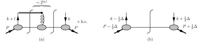
Figure 4: (a) Lowest order diagram for T-odd TMDs in spectator model calculations containing the interaction of the active quark with the target remnant. The eikonal propagator arising from the Wilson line in the operator definition of TMDs is indicated by a double line. Note that only the imaginary part of the box diagram on the left-hand side (LHS) of the cut is relevant for the calculation of T-odd functions. The Hermitian conjugate diagram (h.c.) is not shown. (b) Lowest order diagram for GPDs in spectator model calculations. The topology of diagram (a) matches with the one of diagram (b) if the quark-spectator interaction, described by the lensing function $\mathcal{I}^{q,i}$, is factored out.

The discussion in Sec. IV B and IV C was exclusively devoted to the relations of second type. Here we want to consider the relations of third type indicated in (76) and (84). As already pointed out in Sec. III C one can expect the specific form of possible relations of third type to be different from the relations of second type. This expectation is also supported by the fact that all the TMDs in (III.3) and (III.4) are T-odd, while in (76) and (84) they are T-even. To the best of our knowledge an explicit form of a relation of third type does not exist in the literature.

Analogous to the result in (IV.3) a general relation between the moments of TMDs and the moments of GPDs can be established. To be specific the diquark spectator model results for $h_{1T}^{\bot q}$ in (129) and for $\tilde{H}_{T}^{q}$ in (138) obey

$$h_{1T}^{\bot q\,(n)}(x)$$

$$\ =-\frac{g^{2}(1-x)}{4(2\pi)}\,\frac{n\tilde{M}^{2n-2}(x)}{2^{n}M^{2n-2}\,\sin(n\pi)}$$

$$\ =\frac{1}{(2\pi)\,(1-x)^{2}}\,\frac{n\,\Gamma(4-2n)}{\Gamma^{2}(2-n)}\,\tilde{H}_{T}^{q\,(n)}(x)\,,$$ (109)

which again holds for $0\leq n\leq 1$. The corresponding quark distributions in the quark target model fulfill exactly the same relation. Notice that here no replacement of the type (103) is needed when making the transition from the scalar diquark model to the quark target model because the T-even TMDs and the GPDs in Eq. (IV.4) receive the first nonzero contribution at the same order in perturbation theory. In addition, we find that those gluon distributions in the quark target model, which enter the relation of third type as indicated in (84), satisfy a relation with exactly the structure of (IV.4).

As expected, the general structure of the relation in (IV.3) and in (IV.4) is different. Note that due to the Wilson line contribution to the T-odd TMDs, the prefactor on the RHS in (IV.3) contains couplings which do not appear in (IV.4). Moreover, the relative power of $(1-x)$ between the moments of the TMDs and of the GPDs differs for both types of relations.

Evaluating (IV.4) for three specific values of $n$ one finds

$$h_{1T}^{\bot q\,(0)}(x) =\frac{3}{(1-x)^{2}}\,\tilde{H}_{T}^{q}(x,0,0)\,,$$ (110)

$$h_{1T}^{\bot q\,(1/2)}(x) =\frac{8}{(2\pi)^{2}\,(1-x)^{2}}\,\tilde{H}_{T}^{q\,(1/2)}(x)\,,$$ (111)

$$h_{1T}^{\bot q\,(1)}(x) =\frac{1}{(2\pi)\,(1-x)^{2}}\,\tilde{H}_{T}^{q\,(1)}(x)\,.$$ (112)

Equations (110)–(112) are the counterparts of the relations of second type in (104)–(106).

Keeping in mind the discussion in Sec. III C [see in particular (76)] one may wonder if the relation of third type in (IV.4) can be rewritten such that the second derivative of the impact parameter distribution $\mathcal{\tilde{H}}_{T}^{q}$ shows up. This is indeed possible for arbitrary values of $n$. Instead of providing a general formula we limit this discussion to the particular case $n=1$ in which the most compact and appealing result follows. To this end we exploit the model-independent identity

$$\int d^{2}\vec{b}_{T}\,\frac{\vec{b}_{T}^{\,2}}{2M^{2}}\,2\bigg{(}\mathcal{\tilde{H}}_{T}^{q}(x,\vec{b}_{T}^{\,2})\bigg{)}^{\prime\prime}$$

$$\ =-\pi\int_{0}^{\infty}db_{T}^{2}\,\frac{1}{2M^{2}}\,2\bigg{(}\mathcal{\tilde{H}}_{T}^{q}(x,\vec{b}_{T}^{\,2})\bigg{)}^{\prime}$$

$$\ =\frac{\pi}{M^{2}}\,\mathcal{\tilde{H}}_{T}^{q}(x,0)$$

$$\ =\frac{1}{(2\pi)\,(1-x)^{2}}\,\tilde{H}_{T}^{q\,(1)}(x)\,.$$ (113)

In (IV.4) integration by parts is used in order to perform the first step. Combining now Eqs. (112) and (IV.4) one immediately obtains

$$h_{1T}^{\bot q\,(1)}(x)=\int d^{2}\vec{k}_{T}\,\frac{\vec{k}_{T}^{\,2}}{2M^{2}}\,h_{1T}^{\bot q}(x,\vec{k}_{T}^{\,2})$$

$$\ =\int d^{2}\vec{b}_{T}\,\frac{\vec{b}_{T}^{\,2}}{2M^{2}}\,2\bigg{(}\mathcal{\tilde{H}}_{T}^{q}(x,\vec{b}_{T}^{\,2})\bigg{)}^{\prime\prime}\,.$$ (114)

Note that this relation has a strong similarity to the relations of first type in Eqs. (III.1)–(III.1). Exactly the same result holds for the relation of third type containing the gluon distributions [see (76)], i.e.,

$$h_{1}^{\bot g\,(1)}(x)=\int d^{2}\vec{k}_{T}\,\frac{\vec{k}_{T}^{\,2}}{2M^{2}}\,h_{1}^{\bot g}(x,\vec{k}_{T}^{\,2})$$

$$\ =\int d^{2}\vec{b}_{T}\,\frac{\vec{b}_{T}^{\,2}}{2M^{2}}\,2\bigg{(}\mathcal{E}_{T}^{g}(x,\vec{b}_{T}^{\,2})+2\mathcal{\tilde{H}}_{T}^{g}(x,\vec{b}_{T}^{\,2})\bigg{)}^{\prime\prime}\,.$$ (115)

IV.5 Relation of fourth type

Eventually, the relation of fourth type indicated in (77) and (85) is considered. In the framework of the quark target model calculation at lowest order such a relation is satisfied because both the TMD $h_{1T}^{\bot g}$ and the GPD $\tilde{H}_{T}^{g}$ vanish [see Eqs. (160) and (172)]. In order to obtain nonzero results for those distributions higher order diagrams have to be studied. At present one can say neither if higher order results obey a relation of fourth type nor how the specific form of such a relation could look like. One can only speculate that a possible relation of fourth type may be similar to the relation of second type because in both cases a T-odd TMD enters.

IV.6 Higher order diagrams

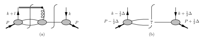
Figure 5: (a) Particular higher order diagram for T-odd TMDs in spectator model calculations containing the interaction of the quark with the target remnants. (b) Topology of diagram (a) if the quark-spectator interaction is factored out. Diagram (b) cannot represent a Feynman graph for a GPD because there is a mismatch between the number of particles on the LHS and the RHS of the cut.

As already pointed out above so far nontrivial relations between GPDs and TMDs are only established if the respective parton distributions are computed in simple spectator models to lowest nontrivial order in perturbation theory. It is therefore natural to ask what happens to the relations if higher order diagrams in spectator models are taken into account. Here we would like to briefly address this point by focusing on the relations of second type.

Consider for instance the relation between the Sivers function and the GPD $E$ as given in Eq. (IV.2). [The following reasoning equally well applies to the relations of second type in (IV.2) and in (IV.2).] We recall that (IV.2) represents a factorization of the Sivers effect into the distortion of the impact parameter dependent distribution of unpolarized quarks in a transversely polarized target, given by the derivative of the GPD $\mathcal{E}^{q}$, times the final state interaction of the active quark, described by the lensing function $\mathcal{I}^{q,i}$.

Pictorially this factorization of the Sivers effect is indicated in Fig. 4. In order to compute the Sivers function to lowest nontrivial order in a spectator model one has to evaluate the cut-diagram in Fig. 4(a). If in this diagram the quark-spectator interaction (lensing function) is factored out, the topology of the remainder coincides with the diagram in Fig. 4(b), which represents a lowest order Feynman graph for a GPD. Hence, it is at least plausible that a factorization as given in Eq. (IV.2) can exist.

Suppose now that higher order diagrams are taken into account for the calculation of the Sivers function, where a particular graph is depicted in Fig. 5(a). Factoring out the quark-spectator interaction in this diagram, one ends up with the topology shown in Fig. 5(b). The diagram in Fig. 5(b), however, does not represent a Feynman graph for a GPD, because the number of particles on the LHS and the RHS of the cut does not match. Therefore, one can expect that even in spectator models the relations of second type no longer hold as soon as higher order diagrams are considered. Of course, strictly speaking our qualitative discussion here only suggests a breakdown of these relations and does not provide a rigorous proof. In any case, in order to arrive at a definite answer on this question a field-theoretic definition of the lensing function is needed. So far no such definition exists.

V Summary

Over the last few years several articles appeared (most notably Refs. Burkardt (2002, 2004a); Burkardt and Hwang (2004); Diehl and Hägler (2005); Burkardt (2005); Brodsky and Gardner (2006); Lu and Schmidt (2007)) suggesting nontrivial relations between generalized and transverse momentum dependent parton distributions. The present work is dealing with this interesting topic and has mainly a twofold purpose: first, a review of the current knowledge on nontrivial relations between GPDs and TMDs is given. Second, the existing results on such relations are considerably extended.

In the following the new results of our work are listed.

1. The correlator for the chiral-odd leading twist gluon GPDs in impact parameter space is written down for the first time [see Eq. (II.2)].

2. A definition of leading twist gluon TMDs is presented which is very similar to the one proposed in Mulders and Rodrigues (2001) and completely analogous to the definition of quark TMDs in Mulders and Tangerman (1996); Boer and Mulders (1998); Goeke et al. (2005); Bacchetta et al. (2007).

3. In the spirit of Ref. Diehl and Hägler (2005) nontrivial relations/analogies between gluon GPDs and TMDs are obtained by comparing the correlators for GPDs in impact parameter representation with the corresponding TMD correlators. This procedure allows one to distinguish between different types of relations/analogies, however does not provide an explicit form of a possible relation. The type of the relation is determined, e.g., by the number of derivatives of the GPDs appearing in the correlator in impact parameter representation (see Sec. III C). In our terminology relations of second, third, and fourth type represent nontrivial connections between GPDs and TMDs. For instance the relation between the Sivers effect and the GPD $E$ proposed in Burkardt (2002, 2004a); Burkardt and Hwang (2004) is called a relation of second type.

4. It is argued that the momentum space representation of GPDs is also suitable in order to find possible relations between GPDs and TMDs. (see Sec. III D).

5. The first calculation of all leading twist GPDs and TMDs in both the scalar diquark model of the nucleon and the quark target model is performed (to lowest nontrivial order in perturbation theory).

6. All our model results, in particular, also those for the gluon distributions, obey the relation of second type [see Eqs. (IV.2), (IV.2), and (IV.2)], where the specific form of this relation was first given in Ref. Burkardt and Hwang (2004).

7. New relations (of second type) for moments of TMDs and GPDs in momentum space (see Sec. IV C) are found, which contain results presented in Refs. Burkardt and Hwang (2004); Lu and Schmidt (2007) as limiting cases.

8. The first explicit form for the relations of third type is given. All our model results fulfill this relation [see Sec. IV D, in particular, the compact results in Eqs. (IV.4) and (IV.4)].

9. The results for the gluon distributions in the quark target model (trivially) satisfy the relation of fourth type in the sense that all involved distributions vanish at the order in perturbation theory considered in our work.

10. It is pointed out that the relations of second type are likely to break down in spectator models if higher order perturbative corrections are taken into consideration.

In very brief terms the general status of nontrivial relations between GPDs and TMDs can be summarized in the following way: so far no model-independent nontrivial relations exist and it seems even unlikely that they can ever be established. On the other hand, many relations exist in the framework of simple spectator models. The phenomenology and the predictive power of the spectator model relation between the Sivers effect and the GPD $E$ works quite well. This is the only relation which so far has been tested to some extent. Additional input from both the experimental and theoretical side is required in order to further study all other relations between GPDs and TMDs. Future work will certainly shed more light on this interesting topic.

Appendix A Scalar diquark model

This appendix contains some elements of the scalar diquark model of the nucleon (see, e.g., Ref. Brodsky et al. (2002a)) and, in particular, the results of the various parton distributions in that approach. Since in the diquark model not only quarks but also diquarks are considered as elementary fields we also provide the definition of GPDs and TMDs for scalar partons in a spin-$\tfrac{1}{2}$ hadron.

The Lagrangian of the diquark model reads

$$\mathcal{L_{\text{SDM}}}(x) =\bar{\Psi}(x)\,(i\gamma^{\mu}\partial_{\mu}-M)\,\Psi(x)+\bar{\psi}(x)\,(i\gamma^{\mu}D_{q,\mu}-m_{q})\,\psi(x)+\varphi^{*}(x)\,(\loarrow{D}_{s}^{\mu*}\,\roarrow{D}_{s,\mu}-m_{s}^{2})\,\varphi(x)$$

$$\quad\,-\tfrac{1}{4}F^{\mu\nu}(x)\,F_{\mu\nu}(x)+g\,\big{[}\bar{\psi}(x)\,\Psi(x)\,\varphi^{*}(x)+\bar{\Psi}(x)\,\psi(x)\,\varphi(x)\big{]}\,,$$ (116)

where $\Psi$ denotes the fermionic target field, $\psi$ the quark field, and $\varphi$ the scalar diquark field. The essential ingredient of the model is a three-point vertex between the target, quarks, and diquarks, with the coupling constant $g$. This framework allows one to carry out perturbative calculations. All the results for parton distributions given below contain the coupling $g$ to the second power, which is the lowest nontrivial order.

In its simplest form the diquark model is of Abelian nature, where both quarks and scalar diquarks couple to a photon field via the covariant derivatives

$$D_{q}^{\mu}\,\psi(x)=\big{[}\partial^{\mu}+ie_{q}\,A^{\mu}(x)\big{]}\,\psi(x)\,,\qquad D_{s}^{\mu}\,\varphi(x)=\big{[}\partial^{\mu}+ie_{s}\,A^{\mu}(x)\big{]}\,\varphi(x)\,,$$ (117)

with the charges $e_{q}$ and $e_{s}$, respectively. In this model the target has no (electromagnetic) charge reflecting the fact that in QCD a hadron is color neutral. This condition directly implies $e_{q}=-e_{s}$ . The field strength tensor of the photon is defined in the standard way by

$$F^{\mu\nu}(x)=\partial^{\mu}A^{\nu}(x)-\partial^{\nu}A^{\mu}(x)\,.$$ (118)

Eventually, we mention that the condition $M<m_{q}+m_{s}$ has to be fulfilled in order to have a stable target state.

For scalar fields only two GPDs ($H^{s}$, $E^{s}$) and two TMDs ($f_{1}^{s}$,  $f_{1T}^{\bot s}$) exist. In analogy with Eqs. (II.1) and (II.1) one defines the leading twist GPDs for scalars according to

$$F^{s}(x,\Delta;\lambda,\lambda^{\prime})$$

$$\ =xP^{+}\int\frac{dz^{-}}{2\pi}\,e^{ik\cdot z}\,\big{<}p^{\prime};\lambda^{\prime}\big{|}\,\varphi^{*}\big{(}\!-\!\tfrac{1}{2}z\big{)}\,\mathcal{W}\big{(}\!-\!\tfrac{1}{2}z;\tfrac{1}{2}z\big{)}\,\varphi\big{(}\tfrac{1}{2}z\big{)}\,\big{|}p;\lambda\big{>}\,\Big{|}\,\!_{\begin{subarray}{c}z^{+}=0^{+}\\ \vec{z}_{T}=\vec{0}_{T}\end{subarray}}$$

$$\ =\frac{1}{2P^{+}}\,\bar{u}(p^{\prime},\lambda^{\prime})\,\bigg{(}\gamma^{+}\,H^{s}(x,\xi,t)+\frac{i\sigma^{+\mu}\Delta_{\mu}}{2M}\,E^{s}(x,\xi,t)\bigg{)}\,u(p,\lambda)\,.$$ (119)

The correlator in impact parameter representation (at $\xi=0$) is given by

$$\mathcal{F}^{s}(x,\vec{b}_{T};S)=\mathcal{H}^{s}(x,\vec{b}_{T}^{\,2})+\frac{\epsilon_{T}^{ij}b_{T}^{i}S_{T}^{j}}{M}\,\bigg{(}\mathcal{E}^{s}(x,\vec{b}_{T}^{\,2})\bigg{)}^{\prime}\,,$$ (120)

i.e., it coincides in its form with Eq. (II.2). The definition of TMDs for scalar fields reads

$$\Phi^{s}(x,\vec{k}_{T};S)$$

$$\ =xP^{+}\int\frac{dz^{-}}{2\pi}\,\frac{d^{2}\vec{z}_{T}}{(2\pi)^{2}}\,e^{ik\cdot z}\,\big{<}P;S\big{|}\,\varphi^{*}\big{(}\!-\!\tfrac{1}{2}z\big{)}\,\mathcal{W}_{+\infty}\big{(}\!-\!\tfrac{1}{2}z;\tfrac{1}{2}z\big{)}\,\varphi\big{(}\tfrac{1}{2}z\big{)}\,\big{|}P;S\big{>}\,\Big{|}_{z^{+}=0^{+}}$$

$$\ =f_{1}^{s}(x,\vec{k}_{T}^{\,2})-\frac{\epsilon^{ij}_{T}k_{T}^{i}S_{T}^{j}}{M}\,f_{1T}^{s}(x,\vec{k}_{T}^{\,2})\,,$$ (121)

and is analogous to Eqs. (II.3) and (II.3). We also note that in the diquark model an obvious change in the definition of the Wilson lines in the different parton correlation functions appears: instead of the strong coupling $g$ the charges $-e_{q}$ and $-e_{s}$ have to be used in the correlators of quark and scalar diquark distributions, respectively.

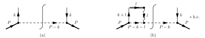
Figure 6: Cut diagrams contributing to quark TMDs and GPDs in the scalar diquark model: (a) diagram for T-even TMDs and GPDs; (b) diagram for T-odd TMDs. Note that in the case of GPDs the kinematics of Fig. 1 has to be used.

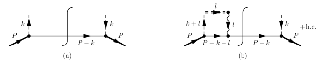
Figure 7: Cut diagrams contributing to diquark TMDs and GPDs in the scalar diquark model: (a) diagram for T-even TMDs and GPDs; (b) diagram for T-odd TMDs. Note that in the case of GPDs the kinematics of Fig. 1 has to be used.

The perturbative calculation of the TMDs and GPDs in the scalar diquark model is basically straightforward. The parton distributions are given by the diagrams in Figs. 6 and 7. In the following we just quote the final results without providing any details of the calculation. We begin with the TMDs, where our results for T-even functions are of ${\mathcal{O}}(g^{2})$, while the first nontrivial results for T-odd functions exist at ${\mathcal{O}}(g^{2}e_{q}e_{s})$. This difference appears because necessarily a contribution from the gauge link is required in order to generate a nonzero T-odd function. Note that to this order all TMDs for antiquarks vanish identically. For the eight TMDs of quarks and the two TMDs of scalar diquarks one finds

$$f_{1}^{q}(x,\vec{k}_{T}^{\,2}) =\frac{g^{2}(1-x)}{2(2\pi)^{3}}\,\frac{\vec{k}_{T}^{\,2}+(m_{q}+xM)^{2}}{\big{[}\vec{k}_{T}^{\,2}+\tilde{M}^{2}(x)\big{]}\,\!^{2}}\,,$$ (122)

$$f_{1T}^{\bot q}(x,\vec{k}_{T}^{\,2}) =\frac{g^{2}e_{q}e_{s}(1-x)}{4(2\pi)^{4}}\,\frac{(m_{q}+xM)M}{\vec{k}_{T}^{\,2}\,\big{[}\vec{k}_{T}^{\,2}+\tilde{M}^{2}(x)\big{]}}\,\ln\bigg{(}\frac{\vec{k}_{T}^{\,2}+\tilde{M}^{2}(x)}{\tilde{M}^{2}(x)}\bigg{)}\,,$$ (123)

$$g_{1L}^{q}(x,\vec{k}_{T}^{\,2}) =-\frac{g^{2}(1-x)}{2(2\pi)^{3}}\,\frac{\vec{k}_{T}^{\,2}-(m_{q}+xM)^{2}}{\big{[}\vec{k}_{T}^{\,2}+\tilde{M}^{2}(x)\big{]}\,\!^{2}}\,,$$ (124)

$$g_{1T}^{q}(x,\vec{k}_{T}^{\,2}) =\frac{g^{2}(1-x)}{(2\pi)^{3}}\,\frac{(m_{q}+xM)M}{\big{[}\vec{k}_{T}^{\,2}+\tilde{M}^{2}(x)\big{]}\,\!^{2}}\,,$$ (125)

$$h_{1}^{\bot q}(x,\vec{k}_{T}^{\,2}) =\frac{g^{2}e_{q}e_{s}(1-x)}{4(2\pi)^{4}}\,\frac{(m_{q}+xM)M}{\vec{k}_{T}^{\,2}\,\big{[}\vec{k}_{T}^{\,2}+\tilde{M}^{2}(x)\big{]}}\,\ln\bigg{(}\frac{\vec{k}_{T}^{\,2}+\tilde{M}^{2}(x)}{\tilde{M}^{2}(x)}\bigg{)}\,,$$ (126)

$$h_{1L}^{\bot q}(x,\vec{k}_{T}^{\,2}) =-\frac{g^{2}(1-x)}{(2\pi)^{3}}\,\frac{(m_{q}+xM)M}{\big{[}\vec{k}_{T}^{\,2}+\tilde{M}^{2}(x)\big{]}\,\!^{2}}\,,$$ (127)

$$h_{1T}^{q}(x,\vec{k}_{T}^{\,2}) =\frac{g^{2}(1-x)}{2(2\pi)^{3}}\,\frac{\vec{k}_{T}^{\,2}+(m_{q}+xM)^{2}}{\big{[}\vec{k}_{T}^{\,2}+\tilde{M}^{2}(x)\big{]}\,\!^{2}}\,,$$ (128)

$$h_{1T}^{\bot q}(x,\vec{k}_{T}^{\,2}) =-\frac{g^{2}(1-x)}{(2\pi)^{3}}\,\frac{M^{2}}{\big{[}\vec{k}_{T}^{\,2}+\tilde{M}^{2}(x)\big{]}\,\!^{2}}\,,$$ (129)

$$f_{1}^{s}(x,\vec{k}_{T}^{\,2}) =\frac{g^{2}x}{2(2\pi)^{3}}\,\frac{\vec{k}_{T}^{\,2}+\big{(}m_{q}+(1-x)M\big{)}\,\!^{2}}{\big{[}\vec{k}_{T}^{\,2}+\tilde{M}^{2}(1-x)\big{]}\,\!^{2}}\,,$$ (130)

$$f_{1T}^{\bot s}(x,\vec{k}_{T}^{\,2}) =-\frac{g^{2}e_{q}e_{s}x}{4(2\pi)^{4}}\,\frac{\big{(}m_{q}+(1-x)M\big{)}M}{\vec{k}_{T}^{\,2}\,\big{[}\vec{k}_{T}^{\,2}+\tilde{M}^{2}(1-x)\big{]}}\,\ln\bigg{(}\frac{\vec{k}_{T}^{\,2}+\tilde{M}^{2}(1-x)}{\tilde{M}^{2}(1-x)}\bigg{)}\,.$$ (131)

In the above formulas we used the abbreviation

$$\tilde{M}^{2}(x)=(1-x)m_{q}^{2}+xm_{s}^{2}-x(1-x)M^{2}$$ (132)

for some specific combination of mass terms. All results in (122)–(131) were already given in the literature. To be specific, the full list of T-even quark TMDs was computed in Ref. Jakob et al. (1997). The quark Sivers function was considered in Collins (2002); Ji and Yuan (2002) (see also Bacchetta et al. (2004)), and the Boer-Mulders function in Goldstein and Gamberg (2002); Boer et al. (2003b). The result for the Sivers function of the scalar diquark can be found in Ref. Goeke et al. (2006).

Now we proceed to the model results for the GPDs, where in all cases nonzero results are obtained at ${\mathcal{O}}(g^{2})$. Again, to this order all GPDs for antiquarks vanish identically. We limit ourselves to the case $\xi=0$ which is sufficient for the purpose of our work. The results read

$$H^{q}(x,0,-\vec{\Delta}_{T}^{2}) =\frac{g^{2}(1-x)}{2(2\pi)^{3}}\,\int d^{2}\vec{k}_{T}\,\frac{\vec{k}_{T}^{\,2}-\tfrac{1}{4}(1-x)^{2}\vec{\Delta}_{T}^{2}+(m_{q}+xM)^{2}}{D_{\textrm{SDM}}^{q}(x,\vec{\Delta}_{T};\vec{k}_{T})}\,,$$ (133)

$$E^{q}(x,0,-\vec{\Delta}_{T}^{2}) =\frac{g^{2}(1-x)^{2}}{(2\pi)^{3}}\,\int d^{2}\vec{k}_{T}\,\frac{(m_{q}+xM)M}{D_{\textrm{SDM}}^{q}(x,\vec{\Delta}_{T};\vec{k}_{T})}\,,$$ (134)

$$\tilde{H}^{q}(x,0,-\vec{\Delta}_{T}^{2}) =-\frac{g^{2}(1-x)}{2(2\pi)^{3}}\,\int d^{2}\vec{k}_{T}\,\frac{\vec{k}_{T}^{\,2}-\tfrac{1}{4}(1-x)^{2}\vec{\Delta}_{T}^{2}-(m_{q}+xM)^{2}}{D_{\textrm{SDM}}^{q}(x,\vec{\Delta}_{T};\vec{k}_{T})}\,,$$ (135)

$$H_{T}^{q}(x,0,-\vec{\Delta}_{T}^{2}) =-\frac{g^{2}(1-x)}{2(2\pi)^{3}}\,\int d^{2}\vec{k}_{T}\,\frac{\tfrac{\vec{\Delta}_{T}^{2}}{\Delta_{T}^{1}\Delta_{T}^{2}}\big{(}k_{T}^{1}k_{T}^{2}-\tfrac{1}{4}(1-x)^{2}\Delta_{T}^{1}\Delta_{T}^{2}\big{)}-(m_{q}+xM)^{2}}{D_{\textrm{SDM}}^{q}(x,\vec{\Delta}_{T};\vec{k}_{T})}\,,$$ (136)

$$E_{T}^{q}(x,0,-\vec{\Delta}_{T}^{2}) =-\frac{g^{2}(1-x)}{(2\pi)^{3}}\,\int d^{2}\vec{k}_{T}\,\frac{\tfrac{4M^{2}}{\Delta_{T}^{1}\Delta_{T}^{2}}\big{(}k_{T}^{1}k_{T}^{2}-\tfrac{1}{4}(1-x)^{2}\Delta_{T}^{1}\Delta_{T}^{2}\big{)}-(1-x)(m_{q}+xM)M}{D_{\textrm{SDM}}^{q}(x,\vec{\Delta}_{T};\vec{k}_{T})}\,,$$ (137)

$$\tilde{H}_{T}^{q}(x,0,-\vec{\Delta}_{T}^{2}) =\frac{2g^{2}(1-x)}{(2\pi)^{3}}\,\int d^{2}\vec{k}_{T}\,\frac{\tfrac{M^{2}}{\Delta_{T}^{1}\Delta_{T}^{2}}\big{(}k_{T}^{1}k_{T}^{2}-\tfrac{1}{4}(1-x)^{2}\Delta_{T}^{1}\Delta_{T}^{2}\big{)}}{D_{\textrm{SDM}}^{q}(x,\vec{\Delta}_{T};\vec{k}_{T})}\,,$$ (138)

$$H^{s}(x,0,-\vec{\Delta}_{T}^{2}) =\frac{g^{2}x}{2(2\pi)^{3}}\,\int d^{2}\vec{k}_{T}\,\frac{\vec{k}_{T}^{\,2}-\tfrac{1}{4}(1-x)^{2}\vec{\Delta}_{T}^{2}+\big{(}m_{q}+(1-x)M\big{)}\,\!^{2}}{D_{\textrm{SDM}}^{s}(x,\vec{\Delta}_{T};\vec{k}_{T})}\,,$$ (139)

$$E^{s}(x,0,-\vec{\Delta}_{T}^{2}) =-\frac{g^{2}x(1-x)}{(2\pi)^{3}}\,\int d^{2}\vec{k}_{T}\,\frac{\big{(}m_{q}+(1-x)M\big{)}M}{D_{\textrm{SDM}}^{s}(x,\vec{\Delta}_{T};\vec{k}_{T})}\,,$$ (140)

with the denominators

$${D_{\textrm{SDM}}^{q}(x,\vec{\Delta}_{T};\vec{k}_{T})} =\big{[}\big{(}\vec{k}_{T}-\tfrac{1}{2}(1-x)\vec{\Delta}_{T}\big{)}\,\!^{2}+\tilde{M}^{2}(x)\big{]}\,\big{[}\big{(}\vec{k}_{T}+\tfrac{1}{2}(1-x)\vec{\Delta}_{T}\big{)}\,\!^{2}+\tilde{M}^{2}(x)\big{]}\,,$$ (141)

$${D_{\textrm{SDM}}^{s}(x,\vec{\Delta}_{T};\vec{k}_{T})} =\big{[}\big{(}\vec{k}_{T}-\tfrac{1}{2}(1-x)\vec{\Delta}_{T}\big{)}\,\!^{2}+\tilde{M}^{2}(1-x)\big{]}\,\big{[}\big{(}\vec{k}_{T}+\tfrac{1}{2}(1-x)\vec{\Delta}_{T}\big{)}\,\!^{2}+\tilde{M}^{2}(1-x)\big{]}\,.$$ (142)

We refrain from performing the integration upon the transverse quark momentum in the results given in (133)–(140) because this step is actually not needed for studying the relations between GPDs and TMDs. Note also that in the case of $H$ and $\tilde{H}$ the $k_{T}$ integration leads to a (logarithmic) ultraviolet divergence, which is not a peculiarity of the diquark model but rather a well-known feature of light-cone correlation functions. For the other GPDs this integral is finite, which for $E$ is directly obvious and in the remaining cases can be shown by explicit calculation.

Appendix B Quark target model

The second model we are using is a quark target, treated in perturbative QCD. Mainly for two reasons this approach is of interest in the context of our investigation. First, the non-Abelian three-gluon vertex now enters the computation of various parton distributions. Therefore, one has an additional check of relations between GPDs and TMDs, beyond what can be done in the Abelian scalar diquark model. Second, the quark target model allows one to investigate relations between gluon distributions.

The Lagrangian of the quark target model is given by

$$\mathcal{L}_{\text{QTM}}(x)=\bar{\psi}(x)\,(i\gamma^{\mu}D_{\mu}-m)\,\psi(x)-\tfrac{1}{4}F^{\mu\nu}_{a}(x)\,F_{\mu\nu,a}(x)\,,$$ (143)

i.e., it coincides the QCD Lagrangian for the specific case of a single quark flavor. The covariant derivative in (143) reads

$$D^{\mu}\,\psi(x)=\big{[}\partial^{\mu}-ig\,t_{a}\,A^{\mu}_{a}(x)\big{]}\,\psi(x)\,,$$ (144)

while the field strength tensor is defined in Eq. (15).

Figure 8: Cut diagrams contributing to quark TMDs and GPDs in the quark target model: (a) diagrams for T-even TMDs and GPDs; (b) diagram for T-odd TMDs. Note that in the case of GPDs the kinematics of Fig. 1 has to be used.

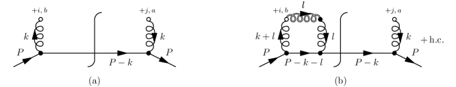
Figure 9: Cut diagrams contributing to gluon TMDs and GPDs in the quark target model: (a) diagram for T-even TMDs and GPDs; (b) diagram for T-odd TMDs. Note that in the case of GPDs the kinematics of Fig. 1 has to be used, and that diagram (b) contains a Wilson line for gluons. The open circle on the upper end of the gluon lines indicates a special Feynman rule for the field strength tensor in the definition of parton distributions for gluons (see Refs. Collins and Soper (1982); Goeke et al. (2006)).

We now list the results for TMDs and GPDs in the quark target model. Like in the case of the diquark model of the nucleon here we also avoid giving any details of the calculation. The relevant diagrams for the quark distributions are depicted in Fig. 8, and those for the gluon distributions in Fig. 9. The T-odd TMDs receive the first nonzero contribution at ${\mathcal{O}}(g^{4})$, while the results for all other distributions (T-even TMDs as well as GPDs) are of ${\mathcal{O}}(g^{2})$.

For the eight TMDs of quarks and the eight TMDs of gluons one finds (in the kinematic region $0<x<1$),

$$f_{1}^{q}(x,\vec{k}_{T}^{\,2}) =\frac{4g^{2}}{3(2\pi)^{3}(1-x)}\,\frac{\big{(}1+x^{2}\big{)}\vec{k}_{T}^{\,2}+(1-x)^{4}\,m^{2}}{\big{[}\vec{k}_{T}^{\,2}+(1-x)^{2}\,m^{2}\big{]}\,\!^{2}}\,,$$ (145)

$$f_{1T}^{\bot q}(x,\vec{k}_{T}^{\,2}) =-\frac{g^{4}x(1-x)}{(2\pi)^{4}}\,\frac{m^{2}}{\vec{k}_{T}^{\,2}\,\big{[}\vec{k}_{T}^{\,2}+(1-x)^{2}\,m^{2}\big{]}}\,\ln\bigg{(}\frac{\vec{k}_{T}^{\,2}+(1-x)^{2}\,m^{2}}{(1-x)^{2}\,m^{2}}\bigg{)}\,,$$ (146)

$$g_{1L}^{q}(x,\vec{k}_{T}^{\,2}) =\frac{4g^{2}}{3(2\pi)^{3}(1-x)}\,\frac{\big{(}1+x^{2}\big{)}\vec{k}_{T}^{\,2}-(1-x)^{4}\,m^{2}}{\big{[}\vec{k}_{T}^{\,2}+(1-x)^{2}\,m^{2}\big{]}\,\!^{2}}\,,$$ (147)

$$g_{1T}^{q}(x,\vec{k}_{T}^{\,2}) =-\frac{8g^{2}x(1-x)}{3(2\pi)^{3}}\,\frac{m^{2}}{\big{[}\vec{k}_{T}^{\,2}+(1-x)^{2}\,m^{2}\big{]}\,\!^{2}}\,,$$ (148)

$$h_{1}^{\bot q}(x,\vec{k}_{T}^{\,2}) =-\frac{g^{4}(1-x)}{(2\pi)^{4}}\,\frac{m^{2}}{\vec{k}_{T}^{\,2}\,\big{[}\vec{k}_{T}^{\,2}+(1-x)^{2}\,m^{2}\big{]}}\,\ln\bigg{(}\frac{\vec{k}_{T}^{\,2}+(1-x)^{2}\,m^{2}}{(1-x)^{2}\,m^{2}}\bigg{)}\,,$$ (149)

$$h_{1L}^{\bot q}(x,\vec{k}_{T}^{\,2}) =\frac{8g^{2}(1-x)}{3(2\pi)^{3}}\,\frac{m^{2}}{\big{[}\vec{k}_{T}^{\,2}+(1-x)^{2}\,m^{2}\big{]}\,\!^{2}}\,,$$ (150)

$$h_{1T}^{q}(x,\vec{k}_{T}^{\,2}) =\frac{8g^{2}x}{3(2\pi)^{3}(1-x)}\,\frac{\vec{k}_{T}^{\,2}}{\big{[}\vec{k}_{T}^{\,2}+(1-x)^{2}\,m^{2}\big{]}\,\!^{2}}\,,$$ (151)

$$h_{1T}^{\bot q}(x,\vec{k}_{T}^{\,2}) =0\,,$$ (152)

$$f_{1}^{g}(x,\vec{k}_{T}^{\,2}) =\frac{4g^{2}}{3(2\pi)^{3}x}\,\frac{\big{(}1+(1-x)^{2}\big{)}\vec{k}_{T}^{\,2}+x^{4}m^{2}}{\big{[}\vec{k}_{T}^{\,2}+x^{2}m^{2}\big{]}\,\!^{2}}\,,$$ (153)

$$f_{1T}^{\bot g}(x,\vec{k}_{T}^{\,2}) =\frac{g^{4}x(1-x)}{(2\pi)^{4}}\,\frac{m^{2}}{\vec{k}_{T}^{\,2}\,\big{[}\vec{k}_{T}^{\,2}+x^{2}m^{2}\big{]}}\,\ln\bigg{(}\frac{\vec{k}_{T}^{\,2}+x^{2}m^{2}}{x^{2}m^{2}}\bigg{)}\,,$$ (154)

$$g_{1L}^{g}(x,\vec{k}_{T}^{\,2}) =\frac{4g^{2}}{3(2\pi)^{3}}\,\frac{\big{(}1+(1-x)\big{)}\vec{k}_{T}^{\,2}+x^{3}m^{2}}{\big{[}\vec{k}_{T}^{\,2}+x^{2}m^{2}\big{]}\,\!^{2}}\,,$$ (155)

$$g_{1T}^{g}(x,\vec{k}_{T}^{\,2}) =-\frac{8g^{2}x(1-x)}{3(2\pi)^{3}}\,\frac{m^{2}}{\big{[}\vec{k}_{T}^{\,2}+x^{2}m^{2}\big{]}\,\!^{2}}\,,$$ (156)

$$h_{1}^{\bot g}(x,\vec{k}_{T}^{\,2}) =\frac{16g^{2}(1-x)}{3(2\pi)^{3}x}\,\frac{m^{2}}{\big{[}\vec{k}_{T}^{\,2}+x^{2}m^{2}\big{]}\,\!^{2}}\,,$$ (157)

$$h_{1L}^{\bot g}(x,\vec{k}_{T}^{\,2}) =0\,,$$ (158)

$$h_{1T}^{g}(x,\vec{k}_{T}^{\,2}) =\frac{2g^{4}x}{(2\pi)^{4}}\,\frac{m^{2}}{\vec{k}_{T}^{\,2}\,\big{[}\vec{k}_{T}^{\,2}+x^{2}m^{2}\big{]}}\,\ln\bigg{(}\frac{\vec{k}_{T}^{\,2}+x^{2}m^{2}}{x^{2}m^{2}}\bigg{)}\,,$$ (159)

$$h_{1T}^{\bot g}(x,\vec{k}_{T}^{\,2}) =0\,.$$ (160)

At the kinematical point $x=1$ there exist additional contributions for some of the parton distributions above, which arise if the on-shell intermediate state in the cut diagram is just the vacuum. Those contributions are neglected here for simplicity. Note that three TMDs in (145)–(160) vanish. It is likely that a higher order calculation provides a nonzero result for these objects. Some of the results in (145)–(160) were already given in the literature. Treatments of the quark TMDs $f_{1}^{q},\;g_{1T}^{q},\;h_{1L}^{\bot q},\;h_{1T}^{q}$ can for instance be found in Mukherjee and Chakrabarti (2001); Kundu and Metz (2001); Collins (2003); Schlegel and Metz (2004); Hautmann (2007). The Sivers function for quarks and gluons was computed in Ref. Goeke et al. (2006).

Eventually, we consider the GPDs in the quark target model. The results (for $\xi=0$ and $0<x<1$) read

$$H^{q}(x,0,-\vec{\Delta}_{T}^{2}) =\frac{4g^{2}}{3(2\pi)^{3}(1-x)}\,\int d^{2}\vec{k}_{T}\,\frac{\big{(}1+x^{2}\big{)}\big{(}\vec{k}_{T}^{\,2}-\tfrac{1}{4}(1-x)^{2}\vec{\Delta}_{T}^{2}\big{)}+(1-x)^{4}\,m^{2}}{D_{\textrm{QTM}}^{q}(x,\vec{\Delta}_{T};\vec{k}_{T})}\,,$$ (161)

$$E^{q}(x,0,-\vec{\Delta}_{T}^{2}) =\frac{8g^{2}x(1-x)^{2}}{3(2\pi)^{3}}\,\int d^{2}\vec{k}_{T}\,\frac{m^{2}}{D_{\textrm{QTM}}^{q}(x,\vec{\Delta}_{T};\vec{k}_{T})}\,,$$ (162)

$$\tilde{H}^{q}(x,0,-\vec{\Delta}_{T}^{2}) =\frac{4g^{2}}{3(2\pi)^{3}(1-x)}\,\int d^{2}\vec{k}_{T}\,\frac{\big{(}1+x^{2}\big{)}\big{(}\vec{k}_{T}^{\,2}-\tfrac{1}{4}(1-x)^{2}\vec{\Delta}_{T}^{2}\big{)}-(1-x)^{4}\,m^{2}}{D_{\textrm{QTM}}^{q}(x,\vec{\Delta}_{T};\vec{k}_{T})}\,,$$ (163)

$$H_{T}^{q}(x,0,-\vec{\Delta}_{T}^{2}) =\frac{8g^{2}x}{3(2\pi)^{3}(1-x)}\,\int d^{2}\vec{k}_{T}\,\frac{\vec{k}_{T}^{\,2}-\tfrac{1}{4}(1-x)^{2}\vec{\Delta}_{T}^{2}}{D_{\textrm{QTM}}^{q}(x,\vec{\Delta}_{T};\vec{k}_{T})}\,,$$ (164)

$$E_{T}^{q}(x,0,-\vec{\Delta}_{T}^{2}) =\frac{8g^{2}(1-x)^{2}}{3(2\pi)^{3}}\,\int d^{2}\vec{k}_{T}\,\frac{m^{2}}{D_{\textrm{QTM}}^{q}(x,\vec{\Delta}_{T};\vec{k}_{T})}\,,$$ (165)

$$\tilde{H}_{T}^{q}(x,0,-\vec{\Delta}_{T}^{2}) =0\,,$$ (166)

$$H^{g}(x,0,-\vec{\Delta}_{T}^{2}) =\frac{4g^{2}}{3(2\pi)^{3}x}\,\int d^{2}\vec{k}_{T}\,\frac{\big{(}1+(1-x)^{2}\big{)}\big{(}\vec{k}_{T}^{\,2}-\tfrac{1}{4}(1-x)^{2}\vec{\Delta}_{T}^{2}\big{)}+x^{4}m^{2}}{D_{\textrm{QTM}}^{g}(x,\vec{\Delta}_{T};\vec{k}_{T})}\,,$$ (167)

$$E^{g}(x,0,-\vec{\Delta}_{T}^{2}) =-\frac{8g^{2}x(1-x)^{2}}{3(2\pi)^{3}}\,\int d^{2}\vec{k}_{T}\,\frac{m^{2}}{D_{\textrm{QTM}}^{g}(x,\vec{\Delta}_{T};\vec{k}_{T})}\,,$$ (168)

$$\tilde{H}^{g}(x,0,-\vec{\Delta}_{T}^{2}) =\frac{4g^{2}}{3(2\pi)^{3}}\,\int d^{2}\vec{k}_{T}\,\frac{\big{(}1+(1-x)\big{)}\big{(}\vec{k}_{T}^{\,2}-\tfrac{1}{4}(1-x)^{2}\vec{\Delta}_{T}^{2}\big{)}+x^{3}m^{2}}{D_{\textrm{QTM}}^{g}(x,\vec{\Delta}_{T};\vec{k}_{T})}\,,$$ (169)

$$H_{T}^{g}(x,0,-\vec{\Delta}_{T}^{2}) =-\frac{8g^{2}x(1-x)}{3(2\pi)^{3}}\,\int d^{2}\vec{k}_{T}\,\frac{m^{2}}{D_{\textrm{QTM}}^{g}(x,\vec{\Delta}_{T};\vec{k}_{T})}\,,$$ (170)

$$E_{T}^{g}(x,0,-\vec{\Delta}_{T}^{2}) =-\frac{32g^{2}(1-x)}{3(2\pi)^{3}x}\,\int d^{2}\vec{k}_{T}\,\frac{\tfrac{m^{2}}{\Delta_{T}^{1}\Delta_{T}^{2}}\,\big{(}k_{T}^{1}k_{T}^{2}-\tfrac{1}{4}(1-x)^{2}\Delta_{T}^{1}\Delta_{T}^{2}\big{)}}{D_{\textrm{QTM}}^{g}(x,\vec{\Delta}_{T};\vec{k}_{T})}\,,$$ (171)

$$\tilde{H}_{T}^{g}(x,0,-\vec{\Delta}_{T}^{2}) =0\,,$$ (172)

with the denominators

$${D_{\textrm{QTM}}^{q}(x,\vec{\Delta}_{T};\vec{k}_{T})} =\big{[}\big{(}\vec{k}_{T}-\tfrac{1}{2}(1-x)\vec{\Delta}_{T}\big{)}\,\!^{2}+(1-x)^{2}\,m^{2}\big{]}\,\big{[}\big{(}\vec{k}_{T}+\tfrac{1}{2}(1-x)\vec{\Delta}_{T}\big{)}\,\!^{2}+(1-x)^{2}\,m^{2}\big{]}\,,$$ (173)

$${D_{\textrm{QTM}}^{g}(x,\vec{\Delta}_{T};\vec{k}_{T})} =\big{[}\big{(}\vec{k}_{T}-\tfrac{1}{2}(1-x)\vec{\Delta}_{T}\big{)}\,\!^{2}+x^{2}m^{2}\big{]}\,\big{[}\big{(}\vec{k}_{T}+\tfrac{1}{2}(1-x)\vec{\Delta}_{T}\big{)}\,\!^{2}+x^{2}m^{2}\big{]}\,.$$ (174)

Calculations of the chiral-even GPDs for both quarks and gluons can be found in Refs. Mukherjee and Vanderhaeghen (2002, 2003); Chakrabarti and Mukherjee (2005). To our knowledge the results for the chiral-odd GPDs in (161)–(172) are given here for the first time.

References

• Mueller et al. (1994) D. Müller, D. Robaschik, B. Geyer, F. M. Dittes, and J. Horejsi, Fortschr. Phys. 42, 101 (1994), eprint hep-ph/9812448.
• Diehl (2003) M. Diehl, Phys. Rept. 388, 41 (2003), eprint hep-ph/0307382.
• Belitsky and Radyushkin (2005) A. V. Belitsky and A. V. Radyushkin, Phys. Rept. 418, 1 (2005), eprint hep-ph/0504030.
• Barone et al. (2002) V. Barone, A. Drago, and P. G. Ratcliffe, Phys. Rept. 359, 1 (2002), eprint hep-ph/0104283.
• Mulders and Tangerman (1996) P. J. Mulders and R. D. Tangerman, Nucl. Phys. B461, 197 (1996), eprint hep-ph/9510301.
• Bacchetta et al. (2007) A. Bacchetta et al., JHEP 02, 093 (2007), eprint hep-ph/0611265.
• Adams et al. (1991a) D. L. Adams et al. (E581), Phys. Lett. B261, 201 (1991a).
• Adams et al. (1991b) D. L. Adams et al. (FNAL-E704), Phys. Lett. B264, 462 (1991b).
• Adams et al. (2004) J. Adams et al. (STAR), Phys. Rev. Lett. 92, 171801 (2004), eprint hep-ex/0310058.
• Adler et al. (2005) S. S. Adler et al. (PHENIX), Phys. Rev. Lett. 95, 202001 (2005), eprint hep-ex/0507073.
• Alexakhin et al. (2005) V. Y. Alexakhin et al. (COMPASS), Phys. Rev. Lett. 94, 202002 (2005), eprint hep-ex/0503002.
• Ageev et al. (2007) E. S. Ageev et al. (COMPASS), Nucl. Phys. B765, 31 (2007), eprint hep-ex/0610068.
• Airapetian et al. (2000) A. Airapetian et al. (HERMES), Phys. Rev. Lett. 84, 4047 (2000), eprint hep-ex/9910062.
• Airapetian et al. (2001) A. Airapetian et al. (HERMES), Phys. Rev. D64, 097101 (2001), eprint hep-ex/0104005.
• Airapetian et al. (2003) A. Airapetian et al. (HERMES), Phys. Lett. B562, 182 (2003), eprint hep-ex/0212039.
• Airapetian et al. (2005a) A. Airapetian et al. (HERMES), Phys. Rev. Lett. 94, 012002 (2005a), eprint hep-ex/0408013.
• Airapetian et al. (2005b) A. Airapetian et al. (HERMES), Phys. Lett. B622, 14 (2005b), eprint hep-ex/0505042.
• Diefenthaler (2005) M. Diefenthaler, AIP Conf. Proc. 792, 933 (2005), eprint hep-ex/0507013.
• Airapetian et al. (2007) A. Airapetian et al. (HERMES), Phys. Lett. B648, 164 (2007), eprint hep-ex/0612059.
• Avakian et al. (2004) H. Avakian et al. (CLAS), Phys. Rev. D69, 112004 (2004), eprint hep-ex/0301005.
• Collins (2002) J. C. Collins, Phys. Lett. B536, 43 (2002), eprint hep-ph/0204004.
• Brodsky et al. (2002a) S. J. Brodsky, D. S. Hwang, and I. Schmidt, Phys. Lett. B530, 99 (2002a), eprint hep-ph/0201296.
• Ji et al. (2005) X. Ji, J.-P. Ma, and F. Yuan, Phys. Rev. D71, 034005 (2005), eprint hep-ph/0404183.
• Ji et al. (2004) X. Ji, J.-P. Ma, and F. Yuan, Phys. Lett. B597, 299 (2004), eprint hep-ph/0405085.
• Collins and Metz (2004) J. C. Collins and A. Metz, Phys. Rev. Lett. 93, 252001 (2004), eprint hep-ph/0408249.
• Sivers (1990) D. W. Sivers, Phys. Rev. D41, 83 (1990).
• Sivers (1991) D. W. Sivers, Phys. Rev. D43, 261 (1991).
• Boer and Mulders (1998) D. Boer and P. J. Mulders, Phys. Rev. D57, 5780 (1998), eprint hep-ph/9711485.
• Efremov et al. (2005) A. V. Efremov, K. Goeke, S. Menzel, A. Metz, and P. Schweitzer, Phys. Lett. B612, 233 (2005), eprint hep-ph/0412353.
• Anselmino et al. (2005a) M. Anselmino et al., Phys. Rev. D71, 074006 (2005a), eprint hep-ph/0501196.
• Anselmino et al. (2005b) M. Anselmino et al., Phys. Rev. D72, 094007 (2005b), eprint hep-ph/0507181.
• Vogelsang and Yuan (2005) W. Vogelsang and F. Yuan, Phys. Rev. D72, 054028 (2005), eprint hep-ph/0507266.
• Collins et al. (2006) J. C. Collins et al., Phys. Rev. D73, 014021 (2006), eprint hep-ph/0509076.
• Anselmino et al. (2005c) M. Anselmino et al. (2005c), eprint hep-ph/0511017.
• Burkardt (2002) M. Burkardt, Phys. Rev. D66, 114005 (2002), eprint hep-ph/0209179.
• Burkardt (2004a) M. Burkardt, Nucl. Phys. A735, 185 (2004a), eprint hep-ph/0302144.
• Burkardt and Hwang (2004) M. Burkardt and D. S. Hwang, Phys. Rev. D69, 074032 (2004), eprint hep-ph/0309072.
• Diehl and Hägler (2005) M. Diehl and P. Hägler, Eur. Phys. J. C44, 87 (2005), eprint hep-ph/0504175.
• Burkardt (2005) M. Burkardt, Phys. Rev. D72, 094020 (2005), eprint hep-ph/0505189.
• Lu and Schmidt (2007) Z. Lu and I. Schmidt, Phys. Rev. D75, 073008 (2007), eprint hep-ph/0611158.
• Burkardt (2000) M. Burkardt, Phys. Rev. D62, 071503 (2000), eprint hep-ph/0005108.
• Ralston and Pire (2002) J. P. Ralston and B. Pire, Phys. Rev. D66, 111501 (2002), eprint hep-ph/0110075.
• Diehl (2002) M. Diehl, Eur. Phys. J. C25, 223 (2002), eprint hep-ph/0205208.
• Burkardt (2003) M. Burkardt, Int. J. Mod. Phys. A18, 173 (2003), eprint hep-ph/0207047.
• Lepage and Brodsky (1980) G. P. Lepage and S. J. Brodsky, Phys. Rev. D22, 2157 (1980).
• Soper (1977) D. E. Soper, Phys. Rev. D15, 1141 (1977).
• Goeke et al. (2005) K. Goeke, A. Metz, and M. Schlegel, Phys. Lett. B618, 90 (2005), eprint hep-ph/0504130.
• Mulders and Rodrigues (2001) P. J. Mulders and J. Rodrigues, Phys. Rev. D63, 094021 (2001), eprint hep-ph/0009343.
• Collins and Soper (1982) J. C. Collins and D. E. Soper, Nucl. Phys. B194, 445 (1982).
• Ji and Yuan (2002) X. Ji and F. Yuan, Phys. Lett. B543, 66 (2002), eprint hep-ph/0206057.
• Belitsky et al. (2003) A. V. Belitsky, X. Ji, and F. Yuan, Nucl. Phys. B656, 165 (2003), eprint hep-ph/0208038.
• Boer et al. (2003a) D. Boer, P. J. Mulders, and F. Pijlman, Nucl. Phys. B667, 201 (2003a), eprint hep-ph/0303034.
• Bomhof et al. (2004) C. J. Bomhof, P. J. Mulders, and F. Pijlman, Phys. Lett. B596, 277 (2004), eprint hep-ph/0406099.
• Bacchetta et al. (2005) A. Bacchetta, C. J. Bomhof, P. J. Mulders, and F. Pijlman, Phys. Rev. D72, 034030 (2005), eprint hep-ph/0505268.
• Bomhof et al. (2006) C. J. Bomhof, P. J. Mulders, and F. Pijlman, Eur. Phys. J. C47, 147 (2006), eprint hep-ph/0601171.
• Bomhof and Mulders (2007) C. J. Bomhof and P. J. Mulders, JHEP 02, 029 (2007), eprint hep-ph/0609206.
• Collins (2003) J. C. Collins, Acta Phys. Polon. B34, 3103 (2003), eprint hep-ph/0304122.
• Gamberg et al. (2006) L. P. Gamberg, D. S. Hwang, A. Metz, and M. Schlegel, Phys. Lett. B639, 508 (2006), eprint hep-ph/0604022.
• Hautmann (2007) F. Hautmann (2007), eprint hep-ph/0702196.
• Ralston and Soper (1979) J. P. Ralston and D. E. Soper, Nucl. Phys. B152, 109 (1979).
• Anselmino et al. (1996) M. Anselmino, M. Boglione, J. Hansson, and F. Murgia, Phys. Rev. D54, 828 (1996), eprint hep-ph/9512379.
• Idilbi et al. (2004) A. Idilbi, X. Ji, J.-P. Ma, and F. Yuan, Phys. Rev. D70, 074021 (2004), eprint hep-ph/0406302.
• Anselmino et al. (2006a) M. Anselmino et al., Phys. Rev. D73, 014020 (2006a), eprint hep-ph/0509035.
• Ma and Wang (2004) J.-P. Ma and Q. Wang, Eur. Phys. J. C37, 293 (2004), eprint hep-ph/0310245.
• Efremov and Teryaev (1982) A. V. Efremov and O. V. Teryaev, Sov. J. Nucl. Phys. 36, 140 (1982).
• Efremov and Teryaev (1985) A. V. Efremov and O. V. Teryaev, Phys. Lett. B150, 383 (1985).
• Qiu and Sterman (1991) J.-W. Qiu and G. Sterman, Phys. Rev. Lett. 67, 2264 (1991).
• Qiu and Sterman (1992) J.-W. Qiu and G. Sterman, Nucl. Phys. B378, 52 (1992).
• Burkardt (2007) M. Burkardt AIP Conf. Proc. 915, 313 (2007), eprint hep-ph/0611256.
• Brodsky and Gardner (2006) S. J. Brodsky and S. Gardner, Phys. Lett. B643, 22 (2006), eprint hep-ph/0608219.
• Brodsky and Yuan (2006) S. J. Brodsky and F. Yuan, Phys. Rev. D74, 094018 (2006), eprint hep-ph/0610236.
• Brodsky et al. (2002b) S. J. Brodsky, P. Hoyer, N. Marchal, S. Peigne, and F. Sannino, Phys. Rev. D65, 114025 (2002b), eprint hep-ph/0104291.
• Pobylitsa (2003) P. V. Pobylitsa (2003), eprint hep-ph/0301236.
• Burkardt (2004b) M. Burkardt, Phys. Rev. D69, 057501 (2004b), eprint hep-ph/0311013.
• Burkardt (2004c) M. Burkardt, Phys. Rev. D69, 091501 (2004c), eprint hep-ph/0402014.
• Anselmino et al. (2006b) M. Anselmino, U. D’Alesio, S. Melis, and F. Murgia, Phys. Rev. D74, 094011 (2006b), eprint hep-ph/0608211.
• Pasquini et al. (2005) B. Pasquini, M. Pincetti, and S. Boffi, Phys. Rev. D72, 094029 (2005), eprint hep-ph/0510376.
• Göckeler et al. (2007) M. Göckeler et al., Phys. Rev. Lett. 98, 222001 (2007), eprint hep-lat/0612032.
• Jakob et al. (1997) R. Jakob, P. J. Mulders, and J. Rodrigues, Nucl. Phys. A626, 937 (1997), eprint hep-ph/9704335.
• Bacchetta et al. (2004) A. Bacchetta, A. Schaefer, and J.-J. Yang, Phys. Lett. B578, 109 (2004), eprint hep-ph/0309246.
• Goldstein and Gamberg (2002) G. R. Goldstein and L. Gamberg (2002), eprint hep-ph/0209085.
• Boer et al. (2003b) D. Boer, S. J. Brodsky, and D. S. Hwang, Phys. Rev. D67, 054003 (2003b), eprint hep-ph/0211110.
• Goeke et al. (2006) K. Goeke, S. Meissner, A. Metz, and M. Schlegel, Phys. Lett. B637, 241 (2006), eprint hep-ph/0601133.
• Mukherjee and Chakrabarti (2001) A. Mukherjee and D. Chakrabarti, Phys. Lett. B506, 283 (2001), eprint hep-ph/0102003.
• Kundu and Metz (2001) R. Kundu and A. Metz, Phys. Rev. D65, 014009 (2001), eprint hep-ph/0107073.
• Schlegel and Metz (2004) M. Schlegel and A. Metz (2004), eprint hep-ph/0406289.
• Mukherjee and Vanderhaeghen (2002) A. Mukherjee and M. Vanderhaeghen, Phys. Lett. B542, 245 (2002), eprint hep-ph/0206159.
• Mukherjee and Vanderhaeghen (2003) A. Mukherjee and M. Vanderhaeghen, Phys. Rev. D67, 085020 (2003), eprint hep-ph/0211386.
• Chakrabarti and Mukherjee (2005) D. Chakrabarti and A. Mukherjee, Phys. Rev. D71, 014038 (2005), eprint hep-ph/0410278.