We study radiative corrections localized at the fixed points of the orbifold for the field theory in six dimensions with two dimensions compactified on the $T_{2}/(Z_{2}\times Z_{2}^{\prime})$ orbifold in a specific realistic model for low energy physics that solves the proton decay and neutrino mass problem. We calculate corrections to the masses of the lightest stable KK modes, which could be the candidates for dark matter.

1 Introduction

One of the important questions in particle physics today is the nature of physics beyond the standard model (SM). The new Large Hadron Collider (LHC) machine starting soon, experiments searching for dark matter of the universe as well as many neutrino experiments planned or under way, have raised the level of excitement in the field since they are poised to provide a unique experimental window into this new physics. The theoretical ideas they are likely to test are supersymmetry, left-right symmetry as well as possible hidden extra dimensions [1][2][3] in nature, which all have separate motivations and address different puzzles of the SM. In this paper, I will focus on an aspect of one interesting class of models known as universal extra dimension models(UED) [4](see for review [5]). These models provide a very different class of new physics at TeV (see [6] for the constraints on size of compactification $R$ ) scale than supersymmetry. But in general UED models based on the standard model gauge group, there is no simple explanation for the suppressed proton decay and the small neutrino mass. One way to solve the proton decay problem in the context of total six space-time dimensions, was proposed in [7]. In this case, the additional dimensions lead to the new U(1) symmetry, that suppresses all baryon-number violating operators. The small neutrino masses can be explained by the propagation of the neutrino in the seventh warp extra dimension [8]. On the other hand we can solve both these problems by extending gauge group to the $SU(2)_{L}\times SU(2)_{R}\times U(1)_{B-L}$[9]. Such class of UED models were proposed in [10]. In this case, the neutrino mass is suppressed due to the $B-L$ gauge symmetry and specific orbifolding conditions that keep left-handed neutrinos at zero mode and forbid lower dimensional operators that can lead to the unsuppressed neutrino mass.

An important consequence of UED models is the existence of a new class of dark matter particle, i.e. the lightest KK (Kaluza-Klein) mode[11]. The detailed nature of the dark matter and its consequences for new physics is quite model-dependent. It was shown recently [12] that the lightest stable KK modes in the model [10] with universal extra dimensions could provide the required amount of cold dark matter [13]. Dark matter in this particular class of UED models is an admixture of the KK photon and right-handed neutrinos. In the case of the two extra dimensions, KK mode of the every gauge boson is accompanied by the additional adjoint scalar which has the same quantum numbers as a gauge boson. In the tree level approximation KK masses of this adjoint scalar and gauge boson are the same, so they both can be dark matter candidates. The paper [12] presented relic density analysis assuming either the adjoint scalar or the gauge boson is the lightest stable KK particle. These assumptions lead to the different restrictions on the parameter space. My goal in this work was to find out whether radiative corrections could produce mass splitting of these modes, and if they do, determine the lightest stable one. In this calculations I will follow the works [14],[15]. Similar calculations for different types of orbifolding were considered in [16] ($T^{2}/Z_{4}$ orbifold),and [17]($M_{4}\times S^{1}/Z_{2}$ and $T^{2}/Z_{2}$ orbifolds).

2 Model

In this sections we will review the basic features of the model [10]. The gauge group of the model is $SU(3)_{c}\times SU(2)_{L}\times SU(2)_{R}\times U(1)_{B-L}$ with the following matter content for generation :

$${\cal Q}_{1,-},{\cal Q}^{\prime}_{1,-}=(3,2,1,\tfrac{1}{3}); {\cal Q}_{2,+},{\cal Q}^{\prime}_{2,+}=(3,1,2,\tfrac{1}{3});$$

$${\cal\psi}_{1,-},{\cal\psi}^{\prime}_{1,-}=(1,2,1,-1); {\cal\psi}_{2,+},{\cal\psi}^{\prime}_{2,+}=(1,1,2,-1);$$ (1)

We denote the gauge bosons as $G_{A}$, $W^{\pm}_{L,A}$, $W^{\pm}_{R,A}$, and $B_{A}$, for $SU(3)_{c}$, $SU(2)_{L}$, $SU(2)_{R}$ and $U(1)_{B-L}$ respectively, where $A=0,1,2,3,4,5$ denotes the six space-time indices. We will also use the following short hand notations: Greek letters $\mu,\nu,\dots=0,1,2,3$ for usual four dimensions indices and lower case Latin letters $a,b,\dots=4,5$ for the extra space dimensions.

We compactify the extra $x_{4}$, $x_{5}$ dimensions into a torus, $T^{2}$, with equal radii, $R$, by imposing periodicity conditions, $\varphi(x_{4},x_{5})=\varphi(x_{4}+2\pi R,x_{5})=\varphi(x_{4},x_{5}+2\pi R)$ for any field $\varphi$. We impose the further orbifolding conditions i.e. $Z_{2}:\vec{y}\rightarrow-\vec{y}~{}\mbox{and}~{}Z^{\prime}_{2}:\vec{y}~{}^{\prime}\rightarrow-\vec{y}~{}^{\prime}$ where $\vec{y}=(x_{4},x_{5})$, $\vec{y}~{}^{\prime}=\vec{y}-(\pi R/2,\pi R/2)$. The $Z_{2}$ fixed points will be located at the coordinates $(0,0)$ and $(\pi R,\pi R)$, whereas those of $Z_{2}^{\prime}$ will be in $(\pi R/2,\pm\pi R/2)$. The generic field $\phi(x_{\mu},x_{a})$ with fixed $Z_{2}\times Z_{2}^{\prime}$ parities can be expanded as:

$$\phi(+,+)=\frac{1}{2\pi R}\varphi^{(0,0)}+\frac{1}{\sqrt{2}\pi R}\sum_{n_{4}+n_{5}~{}\text{-even}}\varphi^{(n_{4},n_{5})}(x_{\mu})cos\left(\frac{n_{4}x_{4}+n_{5}x_{5}}{R}\right)$$

$$\phi(+,-)=\frac{1}{\sqrt{2}\pi R}\sum_{n_{4}+n_{5}~{}\text{ -odd}}\varphi^{(n_{4},n_{5})}(x_{\mu})cos\left(\frac{n_{4}x_{4}+n_{5}x_{5}}{R}\right)$$

$$\phi(-,+)=\frac{1}{\sqrt{2}\pi R}\sum_{n_{4}+n_{5}~{}\text{ -odd}}\varphi^{(n_{4},n_{5})}(x_{\mu})sin\left(\frac{n_{4}x_{4}+n_{5}x_{5}}{R}\right)$$

$$\phi(-,-)=\frac{1}{\sqrt{2}\pi R}\sum_{n_{4}+n_{5}~{}\text{ -even}}\varphi^{(n_{4},n_{5})}(x_{\mu})sin\left(\frac{n_{4}x_{4}+n_{5}x_{5}}{R}\right)$$ (2)

One can see that only the $(+,+)$ fields will have zero modes. In the effective 4D theory the mass of each mode has the form: $m_{N}^{2}=m_{0}^{2}+\frac{N}{R^{2}}$; with $N=\vec{n}^{2}=n_{4}^{2}+n_{5}^{2}$ and $m_{0}$ is the physical mass of the zero mode.

We assign the following $Z_{2}\times Z^{\prime}_{2}$ charges to the various fields:

$$G_{\mu}(+,+);\quad B_{\mu}(+,+);\quad W_{L,\mu}^{3,\pm}(+,+);W^{3}_{R,\mu}(+,+);W^{\pm}_{R,\mu}(+,-);$$

$$G_{a}(-,-);\quad B_{a}(-,-);\quad W_{L,a}^{3,\pm}(-,-);W^{3}_{R,a}(-,-);W^{\pm}_{R,a}(-,+).$$ (3)

As a result, the gauge symmetry $SU(3)_{c}\times SU(2)_{L}\times SU(2)_{R}\times U(1)_{B-L}$ breaks down to $SU(3)_{c}\times SU(2)_{L}\times U(1)_{I_{3R}}\times U(1)_{B-L}$ on the 3+1 dimensional brane. The $W^{\pm}_{R}$ picks up a mass $R^{-1}$, whereas prior to symmetry breaking the rest of the gauge bosons remain massless.

For quarks we choose,

$$Q_{1,L}\equiv\left(\begin{array}[]{c}u_{1L}(+,+)\\ d_{1L}(+,+)\end{array}\right); Q^{\prime}_{1,L}\equiv\left(\begin{array}[]{c}u^{\prime}_{1L}(+,-)\\ d^{\prime}_{1L}(+,-)\end{array}\right);$$ (8)

$$Q_{1,R}\equiv\left(\begin{array}[]{c}u_{1R}(-,-)\\ d_{1R}(-,-)\end{array}\right); Q^{\prime}_{1,R}\equiv\left(\begin{array}[]{c}u^{\prime}_{1R}(-,+)\\ d^{\prime}_{1R}(-,+)\end{array}\right);$$ (13)

$$Q_{2,L}\equiv\left(\begin{array}[]{c}u_{2L}(-,-)\\ d_{2L}(-,+)\end{array}\right); Q^{\prime}_{2,L}\equiv\left(\begin{array}[]{c}u^{\prime}_{2L}(-,+)\\ d^{\prime}_{2L}(-,-)\end{array}\right);$$ (18)

$$Q_{2,R}\equiv\left(\begin{array}[]{c}u_{2R}(+,+)\\ d_{2R}(+,-)\end{array}\right); Q^{\prime}_{2,R}\equiv\left(\begin{array}[]{c}u^{\prime}_{2R}(+,-)\\ d^{\prime}_{2R}(+,+)\end{array}\right);$$ (23)

and for leptons:

$$\psi_{1,L}\equiv\left(\begin{array}[]{c}\nu_{1L}(+,+)\\ e_{1L}(+,+)\end{array}\right); \psi^{\prime}_{1,L}\equiv\left(\begin{array}[]{c}\nu^{\prime}_{1L}(-,+)\\ e^{\prime}_{1L}(-,+)\end{array}\right);$$ (28)

$$\psi_{1,R}\equiv\left(\begin{array}[]{c}\nu_{1R}(-,-)\\ e_{1R}(-,-)\end{array}\right); \psi^{\prime}_{1,R}\equiv\left(\begin{array}[]{c}\nu^{\prime}_{1R}(+,-)\\ e^{\prime}_{1R}(+,-)\end{array}\right);\qquad$$ (33)

$$\psi_{2,L}\equiv\left(\begin{array}[]{c}\nu_{2L}(-,+)\\ e_{2L}(-,-)\end{array}\right); \psi^{\prime}_{2,L}\equiv\left(\begin{array}[]{c}\nu^{\prime}_{2L}(+,+)\\ e^{\prime}_{2L}(+,-)\end{array}\right);$$ (38)

$$\psi_{2,R}\equiv\left(\begin{array}[]{c}\nu_{2R}(+,-)\\ e_{2R}(+,+)\end{array}\right); \psi^{\prime}_{2,R}\equiv\left(\begin{array}[]{c}\nu^{\prime}_{2R}(-,-)\\ e^{\prime}_{2R}(-,+)\end{array}\right).$$ (43)

The zero modes i.e. (+,+) fields correspond to the standard model fields along with an extra singlet neutrino which is left-handed. They will have zero mass prior to gauge symmetry breaking.

The Higgs sector of the model consists of

$$\phi \equiv\left(\begin{array}[]{cc}\phi^{0}_{u}(+,+)&\phi^{+}_{d}(+,-)\\ \phi^{-}_{u}(+,+)&\phi^{0}_{d}(+,-)\end{array}\right);$$ (46)

$$\chi_{L} \equiv\left(\begin{array}[]{c}\chi^{0}_{L}(-,+)\\ \chi^{-}_{L}(-,+)\end{array}\right);\quad\chi_{R}\equiv\left(\begin{array}[]{c}\chi^{0}_{R}(+,+)\\ \chi^{-}_{R}(+,-)\end{array}\right),$$ (51)

with the charge assignment under the gauge group,

$$\phi = (1,2,2,0),$$

$$\chi_{L} = (1,2,1,-1),\quad\chi_{R}=(1,1,2,-1).$$ (52)

In the limit when the scale of $SU(2)_{L}$ is much smaller than the scale of $SU(2)_{R}$ (that is, $v_{w}\ll v_{R}$) the symmetry breaking occurs in two stages. First $SU(2)_{L}\times SU(2)_{R}\times U(1)\rightarrow SU(2)_{L}\times U(1)_{Y}$, where a linear combination of $B_{B-L}$ and $W_{R}^{3}$, acquire a mass to become $Z^{\prime}$, while orthogonal combination of $B_{B-L}$ remains massless and serves as a gauge boson for residual group $U(1)_{Y}$. In terms of the gauge bosons of $SU(2)_{R}$ and $U(1)_{B-L}$, we have

$$Z^{\prime}_{A}=\frac{g_{R}W_{R,A}^{3}-g_{B-L}B_{B-L,A}}{\sqrt{g_{R}^{2}+g_{B-L}^{2}}},$$

$$B_{Y,A}=\frac{g_{R}B_{B-L,A}+g_{B-L}W_{R,A}^{3}}{\sqrt{g_{R}^{2}+g_{B-L}^{2}}}.$$ (53)

Then we have standard breaking of the electroweak symmetry. A detailed discussion of the spectrum of the zeroth and first KK modes was presented in [12]. The main result of the discussion is that in the tree level approximation only the KK modes $B_{Y,\mu}$ $B_{Y,a}$ and $\nu_{2}$ will be stable and can be considered as candidates for dark matter, and the relic CDM density value leads to the upper limits on $R^{-1}$ of about 400-650 Gev, and the mass of the $M_{Z^{\prime}}\leq 1.5$ Tev. However, radiative corrections can split the KK masses of the $B_{Y,\mu}$ and $B_{Y,a}$, and only the lightest of them will be stable. The goal of this work is to find out which of the two modes is lighter and serves as dark matter.

3 Propagators

To calculate the radiative corrections, we follow the methods presented in Refs. [14] and [15]. We derive the propagators for the scalar, fermion, and vector fields in the $T^{2}/(Z_{2}\times Z_{2}^{\prime})$ orbifold, $\varepsilon$ and $\varepsilon^{\prime}$ are the $Z_{2}$ and $Z_{2}^{\prime}$ parities respectively, so arbitrary field satisfying the boundary conditions

$$\phi(x_{4},x_{5})=\varepsilon\phi(-x_{4},-x_{5})$$

$$\phi(x_{4},x_{5})=\varepsilon^{\prime}\phi(\pi R-x_{4},\pi R-x_{5})$$ (54)

can be decomposed as (we always omit the dependence on 4D coordinates)

$$\phi(x_{4},x_{5}) =\Phi(x_{4},x_{5})+\varepsilon\Phi(-x_{4},-x_{5})$$

$$\quad+\varepsilon^{\prime}\Phi(\pi R-x_{4},\pi R-x_{5})+\varepsilon\varepsilon^{\prime}\Phi(x_{4}-\pi R,x_{5}-\pi R).$$ (55)

The field $\phi$ will automatically satisfy the orbifolding conditions of Eq. (54), and one can easily calculate $\langle 0|\phi(x_{4},x_{5})\phi(x^{\prime}_{4},x^{\prime}_{5})|0\rangle$ in the momentum space. This leads to the following expressions for the propagators of the scalar, gauge and fermion fields. Propagator of the scalar field is given by

$$iD=\frac{i}{4(p^{2}-p_{a}^{2})}\left(1+\varepsilon_{\phi}\varepsilon^{\prime}_{\phi}e^{ip_{a}(\pi R)_{a}}\right)\left(\delta_{p_{a}p^{\prime}_{a}}+\varepsilon_{\phi}\delta_{p_{a}-p^{\prime}_{a}}\right),$$ (56)

where $p_{a}(\pi R)_{a}\equiv\pi R(p_{4}+p_{5})$. Propagator of the gauge boson in($\xi=1$) gauge is

$$iD_{AB}=\frac{-ig_{AB}}{4(p^{2}-p_{a}^{2})}\left(1+\varepsilon_{A}\varepsilon_{A}^{\prime}e^{ip_{a}(\pi R)_{a}}\right)\left(\delta_{p_{a}p^{\prime}_{a}}+\varepsilon_{A}\delta_{p_{a}-p^{\prime}_{a}}\right),$$ (57)

where fields $A_{a}$ and $A_{\mu}$ will have opposite $Z_{2}\times Z_{2}^{\prime}$ parities: ($\varepsilon_{\mu}=-\varepsilon_{a},~{}\varepsilon^{\prime}_{\mu}=-\varepsilon^{\prime}_{a}$). The fermion propagator is given by

$$iS_{F}=\frac{i}{4(\mathord{\not\mathrel{{\mathrel{p}}}}-\mathord{\not\mathrel{{\mathrel{p_{a}^{\prime}}}}})}\left(1+\varepsilon_{\psi}\varepsilon^{\prime}_{\psi}e^{ip_{a}(\pi R)_{a}}\right)\left(\delta_{p_{a}p_{a}^{\prime}}+\Sigma_{45}\varepsilon_{\psi}\delta_{p_{a}-p_{a}^{\prime}}\right),$$ (58)

where we have defined

$$\mathord{\not\mathrel{{\mathrel{p_{a}}}}}\equiv p_{4}\Gamma_{4}+p_{5}\Gamma_{5}.$$ (59)

4 Radiative corrections to the fermion mass

Now we want to find corrections for the mass of the $\nu_{2}$ field. First let us consider general interaction between a fermion and a vector boson,

$$\mathcal{L}_{int}=g_{6D}\overline{\psi}\Gamma_{A}\psi A^{A},$$ (60)

where $g_{6D}$ is 6 dimensional coupling constant that is related to the 4 dimensional coupling $g$ by

$$g=\frac{g_{6D}}{(2\pi R)}.$$ (61)

The gauge interaction will give mass corrections due to the diagram Fig.1 (a).

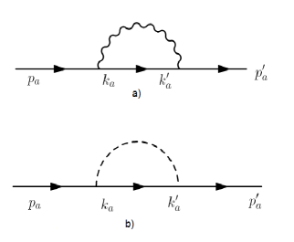
Figure 1: Fermion self energy diagrams

The matrix element will be proportional to the

$$i\Sigma =-\sum_{k_{a}}g^{2}\int\frac{d^{4}k}{(2\pi)^{4}}\frac{1}{4}\frac{1}{(p-k)^{2}-(p_{a}-k_{a})^{2}}$$

$$\quad\quad\times\Gamma_{A}\frac{\mathord{\not\mathrel{{\mathrel{k}}}}-\mathord{\not\mathrel{{\mathrel{k_{a}^{\prime}}}}}}{k^{2}-k_{a}^{2}}[\delta_{k^{\prime}_{a}k_{a}}+\varepsilon_{\psi}\Sigma_{45}\delta_{-k^{\prime}_{a},k_{a}}]\Gamma^{A}[\delta_{(p-k)_{a},(p^{\prime}-k^{\prime})_{a}}+\epsilon^{A}\delta_{(p-k)_{a},-(p^{\prime}-k^{\prime})_{a}}]$$ (62)

The $\varepsilon_{\psi}$ and $\varepsilon^{\prime}_{\psi}$, are the $Z_{2}\times Z_{2}^{\prime}$ parities of the fermion and $\varepsilon^{A}~{},{\varepsilon^{A}}^{\prime}$ are the parities of the gauge boson. The sum is only over the $k_{a}$ which are allowed by the $Z_{2}\times Z_{2}^{\prime}$ parities i.e. for the ones where $1+\varepsilon_{\psi}\varepsilon_{\psi}^{\prime}e^{ik_{a}(\pi R)_{a}}\neq 0$

There are two types of terms that can lead to the corrections of the fermion self energy, the bulk terms appearing due to the nonlocal Lorentz breaking effects and brane like terms which appear because of the specific orbifold conditions, but the bulk terms for fermion self energy graph appear to vanish (see [15]), so we will concentrate our attention only on the brane like terms. In the case of our $T^{2}/(Z_{2}\times Z_{2}^{\prime})$ orbifold they will be localized at the points $(0,0),~{}(\pi R,\pi R),~{}(\pi R/2,\pm\pi R/2)$ (see Appendix). The numerator of the integrand simplifies to

$$\Gamma_{A}(\mathord{\not\mathrel{{\mathrel{k}}}}-\mathord{\not\mathrel{{\mathrel{k_{a}^{\prime}}}}})\Gamma^{A}\varepsilon^{A}\delta_{(p+p^{\prime})_{a},2k_{a}}+\Gamma_{A}(\mathord{\not\mathrel{{\mathrel{k}}}}-\mathord{\not\mathrel{{\mathrel{k_{a}^{\prime}}}}})\Sigma_{45}\Gamma^{A}\varepsilon_{\psi}\delta_{(p-p^{\prime})_{a},2k_{a}}$$

$$=4\mathord{\not\mathrel{{\mathrel{k_{a}^{\prime}}}}}\varepsilon^{\mu}\delta_{p_{a}+p^{\prime}_{a},2k_{a}}+4\mathord{\not\mathrel{{\mathrel{k_{a}^{\prime}}}}}\varepsilon_{\psi}\Sigma_{45}\delta_{2k_{a},p_{a}-p^{\prime}_{a}}$$ (63)

We can then write Eq. (62) as

$$i\Sigma =-\sum_{k_{a}^{\prime}}\frac{g^{2}}{4}\int\frac{d^{4}k}{(2\pi)^{4}}\frac{4\mathord{\not\mathrel{{\mathrel{k_{a}^{\prime}}}}}(\varepsilon^{\mu}\delta_{p_{a}+p^{\prime}_{a},2k_{a}}+\varepsilon_{\psi}\Sigma_{45}\delta_{2k_{a},p_{a}-p^{\prime}_{a}})}{((p-k)^{2}-(p_{a}-k_{a})^{2})(k^{2}-k_{a}^{2})}$$

$$=\frac{-ig^{2}}{2(4\pi)^{2}}\ln\left(\frac{\Lambda^{2}}{\mu^{2}}\right)\left[\frac{\mathord{\not\mathrel{{\mathrel{p_{a}}}}}+\mathord{\not\mathrel{{\mathrel{p^{\prime}_{a}}}}}}{2}(1+\varepsilon_{\psi}\varepsilon_{\psi}^{\prime}e^{(p_{a}+p^{\prime}_{a})(\pi R)_{a}/2})\varepsilon^{\mu}+\varepsilon_{\psi}\frac{\mathord{\not\mathrel{{\mathrel{p^{\prime}_{a}}}}}-\mathord{\not\mathrel{{\mathrel{p_{a}}}}}}{2}(1+\varepsilon_{\psi}\varepsilon_{\psi}^{\prime}e^{(p_{a}-p^{\prime}_{a})(\pi R)_{a}/2})\Sigma_{45}\right],$$ (64)

where $\Lambda$ is a cut-off and $\mu$ is renormalization scale. After transforming to the position space we get

$$\delta\mathcal{L} =\frac{g^{2}}{8(4\pi)^{2}}\ln\left(\frac{\Lambda^{2}}{\mu^{2}}\right)\left[\delta(I)\{\overline{\psi}({i\mathord{\not\mathrel{{\mathrel{\partial_{a}}}}}})(-\varepsilon_{\psi}\Sigma_{45}+\varepsilon^{\mu})\psi+\overline{\psi}{(i{\overleftarrow{\mathord{\not\mathrel{{\mathrel{\partial_{a}}}}}}})}(-\varepsilon_{\psi}\Sigma_{45}-\varepsilon^{\mu})\psi\}\right.$$

$$\quad\quad\quad+\left.\delta(II)\{\overline{\psi}({i\mathord{\not\mathrel{{\mathrel{\partial_{a}}}}}})(-\varepsilon^{\prime}_{\psi}\Sigma_{45}+\varepsilon^{\mu})\psi+\overline{\psi}{(i{\overleftarrow{\mathord{\not\mathrel{{\mathrel{\partial_{a}}}}}}})}(-\varepsilon^{\prime}_{\psi}\Sigma_{45}-\varepsilon^{\mu})\psi\}\right],$$ (65)

where

$$\delta(I)\equiv\delta(x_{a})+\delta(x_{a}-\pi R),~{}~{}\delta(II)\equiv\delta(x_{a}-\pi R/2)+\delta(x_{a}+\pi R/2),$$ (66)

and $\psi$ is normalized as four dimensional fermion field related to the six dimensional field by $\psi=\psi^{6D}(2\pi R)$. In our case the corrections to the self energy of the neutrino will arise from the diagrams with $W^{+}_{R}$, $Z^{\prime}$, but one can see that these fields have nonzero mass coming from the breaking of $SU(2)_{R}$, thus in Eq. (64) $\tilde{p}^{2}\rightarrow\tilde{p}^{2}+(1-\alpha)M^{2}_{W^{\pm}_{R},Z^{\prime}}$. The contribution of the diagram with $W^{\pm}_{R}$ will be

$$\delta\mathcal{L}=\frac{g_{R}^{2}}{8(4\pi)^{2}}\ln\left(\frac{\Lambda^{2}}{\mu_{W_{R}}^{2}}\right)\left[\delta(I)\{\overline{\nu_{2}^{R}}(-\partial_{4}-i\partial_{5})\nu_{2}^{L}+(-\partial_{4}+i\partial_{5})\overline{\nu_{2}^{L}}\nu_{2}^{R}\}\right.$$

$$+\left.\delta(II)\{\overline{\nu_{2}^{L}}(-\partial_{4}+i\partial_{5})\nu_{2}^{R}+(-\partial_{4}-i\partial_{5})\overline{\nu_{2}^{R}}\nu_{2}^{L}\}\right],$$ (67)

where $\mu_{W_{R}}^{2}\sim\mu^{2}+M^{2}_{W_{R}}$. The terms proportional to the $\delta(I)$ and $\delta(II)$ will lead to the corrections to the four dimensional action that will have equal magnitude and opposite sign, so the total correction to the fermion mass will vanish. The contribution of the diagram with $Z^{\prime}$ will lead to the

$$\delta\mathcal{L}=\frac{g_{R}^{2}+g_{B-L}^{2}}{16(4\pi)^{2}}\ln\left(\frac{\Lambda^{2}}{\mu_{Z^{\prime}}^{2}}\right)\left[\delta(I)\{\overline{\nu_{2}^{R}}(-\partial_{4}-i\partial_{5})\nu_{2}^{L}+(-\partial_{4}+i\partial_{5})\overline{\nu_{2}^{L}}\nu_{2}^{R}\}\right.$$

$$+\left.\delta(II)\{\overline{\nu_{2}^{L}}(\partial_{4}-i\partial_{5})\nu_{2}^{R}+(\partial_{4}+i\partial_{5})\overline{\nu_{2}^{R}}\nu_{2}^{L}\}\right],$$ (68)

where $\mu_{Z^{\prime}}^{2}\sim\mu^{2}+M^{2}_{Z^{\prime}}$. Let us look on the first term of the formula (4), it is proportional to the $\delta(I)\overline{\nu_{2}^{R}}\partial_{a}\nu_{2}^{L}$, but one can see from the KK decomposition (2), that profiles of the $\nu_{2}^{R}(+,-)$ and $\partial_{a}\nu_{2}^{L}(-,+)$ are both equal to the $\text{cos}(\frac{n_{4}x_{4}+n_{5}x_{5}}{R})$ i.e. are maximal at the $\delta(I)$. The same is true for the others terms of the (4), thus the correction to the effective 4D lagrangian, and KK masses will be

$$\mathcal{L}_{4D}=\frac{g_{R}^{2}+g_{B-L}^{2}}{4(4\pi)^{2}}\ln\left(\frac{\Lambda^{2}}{\mu_{Z^{\prime}}^{2}}\right)\left[\left(\frac{-n_{4}-in_{5}}{R}\right)\overline{\nu_{2}^{R}}\nu_{2}^{L}+\left(\frac{-n_{4}+in_{5}}{R}\right)\overline{\nu_{2}^{L}}\nu_{2}^{R}\right]$$

$$\delta m_{\nu(n_{4},n_{5})}=\frac{(g_{R}^{2}+g_{B-L}^{2})\sqrt{n_{4}^{2}+n_{5}^{2}}}{4R(4\pi)^{2}}\ln\left(\frac{\Lambda^{2}}{\mu_{Z^{\prime}}^{2}}\right).$$ (69)

So the correction to the mass of the first KK mode for $\nu_{2}$ will be:

$$\delta m_{\nu}=\frac{(g_{R}^{2}+g_{B-L}^{2})}{4R(4\pi)^{2}}\ln\left(\frac{\Lambda^{2}}{\mu_{Z^{\prime}}^{2}}\right).$$ (70)

Now we have to evaluate contribution of the diagram Fig.1 (b)

$$i\Sigma=\sum_{k_{a}}f^{2}\int\frac{d^{4}k}{(2\pi)^{4}}\frac{1}{4}\frac{1}{(p-k)^{2}-(p_{a}-k_{a})^{2}}\frac{\mathord{\not\mathrel{k}}-\mathord{\not\mathrel{k_{a}^{\prime}}}}{k^{2}-k_{a}^{2}}[\varepsilon_{\psi}\Sigma_{45}\delta_{p_{a}-p_{a}^{\prime},2k_{a}}+\varepsilon_{\phi}\delta_{p_{a}+p_{a}^{\prime},2k_{a}}],$$ (71)

where $f$ is the 4D Yukawa coupling , and again we will consider only the terms that are localized at the fixed points of the orbifold.

$$i\Sigma=\sum_{k_{a}}f^{2}\int\frac{d^{4}k}{(2\pi)^{4}}\frac{1}{4}\int_{0}^{1}d\alpha\frac{(\mathord{\not\mathrel{k}}-\mathord{\not\mathrel{k_{a}^{\prime}}})[\varepsilon_{\psi}\Sigma_{45}\delta_{p_{a}-p_{a}^{\prime},2k_{a}}+\varepsilon_{\phi}\delta_{p_{a}+p_{a}^{\prime},2k_{a}}]}{[k^{2}-k_{a}^{2}(1-\alpha)-2(kp)\alpha+p^{2}\alpha-(p_{a}-k_{a})^{2}\alpha]^{2}}$$ (72)

Proceeding in the same wave as we have done for the diagram with the vector field we find

$$i\Sigma=\frac{if^{2}}{16(4\pi)^{2}}\ln\left(\frac{\Lambda^{2}}{\mu^{2}}\right)\left[(\mathord{\not\mathrel{{\mathrel{p}}}}-\mathord{\not\mathrel{{\mathrel{p_{a}^{\prime}}}}}+\mathord{\not\mathrel{{\mathrel{p_{a}}}}})\varepsilon_{\psi}\Sigma_{45}(1+\varepsilon_{\psi}\varepsilon^{\prime}_{\psi}e^{(p_{a}-p^{\prime}_{a})(\pi R)_{a}/2})\right.+$$

$$+\left.(\mathord{\not\mathrel{{\mathrel{p}}}}-\mathord{\not\mathrel{{\mathrel{p_{a}^{\prime}}}}}-\mathord{\not\mathrel{{\mathrel{p_{a}}}}})\varepsilon_{\phi}(1+\varepsilon_{\psi}\varepsilon^{\prime}_{\psi}e^{(p_{a}+p^{\prime}_{a})(\pi R)_{a}/2})\right].$$ (73)

In our model we have the following Yukawa couplings

$$\overline{\psi}_{1}^{-}\Phi\psi_{2}^{+}=\overline{\nu}_{1}\Phi_{d}^{0}\nu_{2}+\overline{e}_{1}\Phi_{d}^{-}\nu_{2}+\overline{\nu}_{1}\Phi_{u}^{+}e_{2}+\overline{e}_{1}\Phi_{u}^{0}e_{2}$$ (74)

So the corrections to the self energy of neutrino will arise from the diagrams with $\Phi_{d}^{0}$ and $\Phi_{d}^{-}$. This leads to the following corrections in the lagrangian

$$\delta{\cal L}=\frac{f^{2}}{8(4\pi)^{2}}\ln\left(\frac{\Lambda^{2}}{\mu^{2}}\right)[\delta(I)\{\overline{\nu_{2}^{R}}i\mathord{\not\mathrel{{\mathrel{\partial}}}}\nu_{2}^{R}+\overline{\nu_{2}^{R}}(\partial_{4}+i\partial_{5})\nu_{2}^{L}+(\partial_{4}-i\partial_{5})\overline{\nu_{2}^{L}}\nu_{2}^{R}\}+$$

$$+\delta(II)\{-\overline{\nu_{2}^{L}}i\mathord{\not\mathrel{{\mathrel{\partial}}}}\nu_{2}^{L}+\overline{\nu_{2}^{L}}(\partial_{4}-i\partial_{5})\nu_{2}^{R}+(\partial_{4}+i\partial_{5})\overline{\nu_{2}^{R}}\nu_{2}^{L}\}]$$ (75)

The terms proportional to $\delta(I)$ and $\delta(II)$ lead to the corrections to the four dimensional action that will cancel each other, so the total mass shift due to the diagrams with $\Phi_{d}^{0,-}$ will be equal to zero, thus the mass of the neutrino will be corrected only due to the diagram with the $Z^{\prime}$ boson (70).

5 Corrections to the mass of the gauge boson

As we have mentioned above the dark matter in the model [10] is believed to consist from mixture of the KK photon and right handed neutrinos, so we are interested in the corrections to the masses of the $B_{Y,a}$ and $B_{Y,\mu}$ bosons. The lowest KK excitations of the $B_{Y,a}$ and $B_{Y,\mu}$ fields correspond to $|p_{4}|=|p_{5}|=\frac{1}{R}~{}$, so everywhere in the calculations we set ($p_{4}=p_{5}\equiv\frac{1}{R})$. At the tree level both $B_{Y,a}$ and $B_{Y,\mu}$ fields have the same mass $\frac{\sqrt{2}}{R}$, but radiative corrections can split their mass levels, and only the lightest one of these two will be stable and could be the candidate for the dark matter. In this case the bulk corrections do not vanish by themselves but as was shown in the [15] lead to the same mass corrections for the $B_{Y,\mu}$ and $B_{Y,a}$ fields.

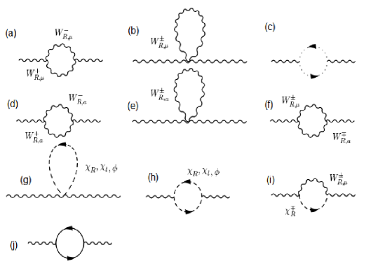
Figure 2: self energy diagrams for the $B_{Y\mu}$ fild:$(a,b)$-loops with $W_{R,mu}^{\pm}$, $(c)$-ghost loop, $(d,e,f)$-loops with $W_{R,-}^{\pm}$, $(g,h,i)$-with goldstone bosons $\chi_{R}^{\pm}$, $(j)$-fermion loop

First we will calculate radiative corrections for the $B_{Y,\mu}$ field (calculations are carried out in the Feynman gauge $\xi=1$ ), see Fig.2 for the list of the relevant diagrams. The contribution of every diagram can be presented in the form:

Table 1: Coefficients A,B,C,D for the self energy diagrams for $B_{Y,\mu}$ from the gauge sector and $\chi_{R}^{\pm}$

Diagram	A	B	C	D
$(a)$	19/3	-22/3	9	18
$(b)$	0	0	-6	-12
$(c)$	1/3	2/3	-1	-2
$(d)$	4/3	-4/3	-4	-8
$(e)$	0	0	4	8
$(f)$	0	0	12	0
$(g)~{}\chi_{R}^{\pm}$	0	0	-2	-4
$(h)~{}\chi_{R}^{\pm}$	-2/3	2/3	2	4
$(i)$	0	0	0	-4
$(j)$	0	0	0	0

$$i\Pi_{\mu\nu}=\frac{i}{4(4\pi)^{2}}\frac{g^{2}_{B-L}g^{2}_{R}}{{g_{R}^{2}+g_{B-L}^{2}}}\ln\left(\frac{\Lambda^{2}}{\mu^{2}_{W_{R}}}\right)$$

$$\times\left[Ap^{2}g_{\mu\nu}+Bp_{\mu}p_{\nu}+C\frac{p_{a}^{2}+p_{a}^{\prime 2}}{2}g_{\mu\nu}+DM_{W_{R}}^{2}g_{\mu\nu}\right]$$ (76)

The coefficients $A,B,C,D$ are listed in the Table 1. The sum of all diagrams is equal to

$$i\Pi_{\mu\nu}=\frac{i}{4(4\pi)^{2}}\frac{g^{2}_{B-L}g^{2}_{R}}{{g_{R}^{2}+g_{B-L}^{2}}}\ln\left(\frac{\Lambda^{2}}{\mu^{2}_{W_{R}}}\right)\left[14g_{\mu\nu}\frac{p_{a}^{2}+p_{a}^{\prime 2}}{2}+\frac{22}{3}(p^{2}g_{\mu\nu}-p_{\mu}p_{\nu})\right].$$ (77)

this leads to the following corrections to the lagrangian

$$\delta\mathcal{L}=\left(-\frac{22}{3}(-\frac{1}{4}F_{\mu\nu}F^{\mu\nu})-7B_{Y\mu}(\partial^{2}_{a}B_{Y}^{\mu})\right)\left[\frac{1}{4(4\pi)^{2}}\frac{g^{2}_{B-L}g^{2}_{R}}{{g_{R}^{2}+g_{B-L}^{2}}}\ln\left(\frac{\Lambda^{2}}{\mu^{2}_{W_{R}}}\right)\right]\left[\frac{\delta(I)-\delta(II)}{4}\right]$$ (78)

These diagrams will not lead to the mass corrections due to the factor $[\delta(I)-\delta(II)]$. The field $B_{Y}$ also interacts with $\chi_{L}$ and $\phi$, because the $U(1)_{Y}$ charge is equal to $Q_{Y}=T^{3}_{R}+\frac{Y_{B-L}}{2}$, where $Y_{B-L}$ is $U(1)_{B-L}$ hypercharge. These diagrams will have the same structure as diagrams (g) and (h), the only difference will be that $\chi_{L}$ and $\phi$ will have no mass from the breaking of $SU(2)_{R}$. The contribution from the fields $\chi_{L}$ and $\phi_{d}^{0,+}$ will have the factor $[\delta(I)-\delta(II)]$, so only the loops with $\phi_{u}^{0,-}$ lead to the nonvanishing result.

$$\delta\mathcal{L}=\frac{1}{12(4\pi)^{2}}\frac{g^{2}_{B-L}g^{2}_{R}}{{g_{R}^{2}+g_{B-L}^{2}}}\ln\left(\frac{\Lambda^{2}}{\mu^{2}}\right)\left[\frac{\delta(I)+\delta(II)}{4}\right]\left(-\frac{1}{4}F_{\mu\nu}F^{\mu\nu}\right)$$

$$\delta m^{2}_{B_{Y,\mu}}=-\frac{1}{12(4\pi)^{2}}\frac{g^{2}_{B-L}g^{2}_{R}}{{g_{R}^{2}+g_{B-L}^{2}}}\frac{2}{R^{2}}\ln\left(\frac{\Lambda^{2}}{\mu^{2}}\right).$$ (79)

Now we will calculate the mass corrections for the $B_{Y,a}$ field. At the tree level the mass matrix of the $B_{Y,a}$ arises from $(-\frac{1}{2}(F_{45})^{2})$, and it has two eigenstates: massless and massive. The massless one is eaten to become the longitudinal component of the KK excitations of the $B_{Y\mu}$ field, and the massive state behaves like 4D scalar, and is our candidate for dark matter. In our case ($p_{4}=p_{5}=\frac{1}{R}$), the $(B_{+}\equiv\frac{B_{4}+B_{5}}{\sqrt{2}})$ is the longitudinal component of the $B_{Y\mu}$, and $B_{-}\equiv\frac{B_{4}-B_{5}}{\sqrt{2}}$ is the massive scalar. Nonvanishing mass corrections will arise only from the loops containing $\phi_{u}^{0,-}$ fields, the other terms will cancel out exactly in the same way as for the $B_{Y\mu}$ field.

$$i\Pi_{ab}=\frac{-i}{4(4\pi)^{2}}\frac{g^{2}_{B-L}g^{2}_{R}}{{g_{R}^{2}+g_{B-L}^{2}}}[p_{c}p^{\prime}_{c}\delta_{ab}-p_{a}p^{\prime}_{b}]\ln\left(\frac{\Lambda^{2}}{\mu^{2}}\right)$$

$$\delta\mathcal{L}=\frac{1}{2}(F_{45})^{2}\left[\frac{1}{4(4\pi)^{2}}\frac{g^{2}_{B-L}g^{2}_{R}}{{g_{R}^{2}+g_{B-L}^{2}}}\ln\left(\frac{\Lambda^{2}}{\mu^{2}}\right)\right]\left[\frac{\delta(I)+\delta(II)}{4}\right]$$

$$\delta m^{2}_{B_{Y-}}=-\frac{1}{4(4\pi)^{2}}\frac{g^{2}_{B-L}g^{2}_{R}}{{g_{R}^{2}+g_{B-L}^{2}}}\frac{2}{R^{2}}\ln\left(\frac{\Lambda^{2}}{\mu^{2}}\right)$$ (80)

Comparing equations (5) and (5), we see that in the one loop approximation $B_{Y-}$ will be the lighter than $B_{Y\mu}$, so our calculations predict that within the model [10], dark matter is admixture of the $B_{Y-}$ and $\nu_{2}$ fields. It is interesting to point out that the same inequality for the radiative corrections to the masses of the gauge bosons was found in the context of model [16].

6 Conclusion

We studied the one-loop structure in the field theory in six dimensions compactified on the $T_{2}/(Z_{2}\times Z_{2}^{\prime})$ orbifold. We showed how to take into account boundary conditions on the $T_{2}/(Z_{2}\times Z_{2}^{\prime})$ orbifold and derived propagators for the fermion, scalar and vector fields. We calculated mass corrections for the fermion and vector fields, and then we applied our results to the lightest stable KK particles in the model [10]. We showed that the lightest stable modes would be, $B_{Y-}$ and $\nu_{2}$ fields. These results are important for the phenomelogical predictions of the model.

Appendix

In the appendix we will show that contribution of the terms, which do not conserve magnitude of the $|p_{a}|$, will lead to the operators localized at the fixed points of the orbifold. We will follow the discussion presented in the work of H.Georgi,A.Grant and G.Hailu [14] and apply it to our case of $T^{2}/(Z_{2}\times Z_{2}^{\prime})$ orbifold. So let us consider general expression.

$$\sum_{p^{\prime}_{a}=p_{a}+\frac{m_{a}}{R}}\frac{1}{2}\left(1+e^{i\pi(m_{4}+m_{5})}\right)\overline{\psi}(p^{\prime})\Gamma\psi(P)$$ (81)

where $\Gamma$ is some generic operator, $\psi$ is six-dimensional fermion field, and factor $1+e^{i\pi(m_{4}+m_{5})}$ appears because initial and final fields have the same ($Z_{2}\times Z_{2}^{\prime}$) parities. The action in the momentum space will be given by

$$S=\sum_{p_{a}}\frac{1}{(2\pi R)^{2}}\sum_{p^{\prime}_{a}=p_{a}+\frac{m_{a}}{R}}\frac{1}{8}\left({1+\varepsilon_{e}\varepsilon^{\prime}_{e}e^{i(\pi R)_{a}p_{a}}}\right)\left({1+e^{i\pi(m_{4}+m_{5})}}\right)\left(1+\varepsilon_{i}\varepsilon^{\prime}_{i}e^{i(\pi R)_{a}k_{a}}\right)\overline{\psi}(p^{\prime})\Gamma\psi(p),$$ (82)

where $\varepsilon_{i,e},~{}\varepsilon^{\prime}_{i,e}$ are the $Z_{2}$ and $Z_{2}^{\prime}$ parities for the particles in the internal and external lines of the diagram respectively, and $k_{a}$ is the momentum of the internal line (we omit integration over the 4D momentum in the expression). Transforming fields $\psi$ to position space we get

$$S=\frac{1}{8(2\pi R)^{2}}\sum_{p_{a}}\sum_{p^{\prime}_{a}=p_{a}+\frac{m_{a}}{R}}\int dx_{a}dx^{\prime}_{a}e^{-ip^{\prime}_{a}x^{\prime}_{a}+ip_{a}x_{a}}\cdot$$

$$\cdot\left[(1+\varepsilon_{e}\varepsilon_{e}^{\prime}e^{i(\pi R)_{a}p_{a}})(1+\varepsilon_{i}\varepsilon^{\prime}_{i}e^{i(\pi R)_{a}(p_{a}\pm p_{a}\pm m_{a}/R)/2})(1+e^{i\pi(m_{4}+m_{5})})\right]\overline{\psi}(x^{\prime})\Gamma\psi(x),$$ (83)

the upper and lower signs in the expression $(1+\varepsilon_{i}\varepsilon_{i}^{\prime}e^{i(\pi R)_{a}(p_{a}\pm p_{a}\pm m_{a}/R)/2})$ correspond to the $k_{a}=\frac{p_{a}\pm p^{\prime}_{a}}{2}$ in the propagator. Now we can use identities:

$$\sum_{p_{a}}\frac{e^{ip_{a}(x_{a}-x^{\prime}_{a})}}{(2\pi R)^{2}}=\delta(x_{a}-x^{\prime}_{a}),$$

$$\sum_{m=-\infty}^{\infty}e^{\frac{imx}{R}}=\sum_{m=-\infty}^{\infty}\delta(m-\frac{x}{2\pi R}).$$ (84)

so

$$S=\frac{1}{4}\int d^{(6)}x~{}\overline{\psi}(x)\Gamma\psi(x)\sum_{m_{a}}\left[\delta(m_{a}-\frac{x_{a}}{2\pi R})+\delta(m_{a}-\frac{1}{2}-\frac{x_{a}}{2\pi R})\right.+$$

$$+\left.\left(\delta(m_{a}-\frac{1}{4}-\frac{x_{a}}{2\pi R})+\delta(m_{a}+\frac{1}{4}-\frac{x_{a}}{2\pi R})\right)\cdot\begin{cases}(\varepsilon_{i}\varepsilon_{i}^{\prime})(\varepsilon_{e}\varepsilon_{e}^{\prime})~{}\text{for }k_{a}=\frac{p_{a}+p^{\prime}_{a}}{2}\\ \varepsilon_{i}\varepsilon_{i}^{\prime}~{}\text{for }k_{a}=\frac{p_{a}-p^{\prime}_{a}}{2}\end{cases}\right]$$ (85)

So the brane terms will be localized at the points $(0,0),(\pi R,\pi R),(\pm\pi R/2,\pm\pi R/2)$.

References

• [1] I. Antoniadis, Phys.Lett. B 246:377-384 (1990).
• [2] I. Antoniadis, N. Arkani-Hamed, S. Dimopoulos and G. R. Dvali, Phys. Lett. B 436: 257 (1998); N. Arkani-Hamed, S. Dimopoulos and G. R. Dvali, Phys. Lett. B 429: 263 (1998)
• [3] D. Cremades, L.E.Ibanez and F.Marchesano, Nucl. Phys. B 643 (2002) 93, C. Kokorelis, Nucl. Phys. B 677 (2004) 115,
• [4] T.Β Appelquist, H.Β C.Β Cheng and B.Β A.Β Dobrescu, β€œBounds on universal extra dimensions,” Phys.Β Rev.Β  D 64, 035002 (2001).
• [5] D.Hooper, S.Profumo, [hep-ph/0701197].
• [6] T. Appelquist, H-U. Yee, Phys.Rev. D 67:055002 (2003)
• [7] T. Appelquist, B.A. Dobrescu, E. Ponton, H-U. Yee, Phys.Rev.Lett. 87:181802 (2001)
• [8] T. Appelquist, B.A. Dobrescu, E. Ponton, H-U. Yee, Phys.Rev. D 65, 105019 (2002).
• [9] J. C. Pati and A. Salam, Phys. Rev. D 10, 275 (1974); R. N. Mohapatra and J. C. Pati, Phys. Rev. D 11, 566, 2558 (1975); G. SenjanoviΔ‡ and R. N. Mohapatra, Phys. Rev. D 12, 1502 (1975).
• [10] R.N.Mohapatra and A.Perez-Lorenzana, Phys.Rev. D 67:075015 (2003)
• [11] G.Β Servant and T.Β M.Β P.Β Tait, Nucl.Β Phys.Β B 650, 391 (2003).
• [12] Ken Hsieh, R.N. Mohapatra, Salah Nasri, Phys. Rev. D 74:066004 (2006); Ken Hsieh, R.N. Mohapatra, Salah Nasri, JHEP 0612:067 (2006)
• [13] H.Β C.Β Cheng, J.Β L.Β Feng and K.Β T.Β Matchev, Phys.Β Rev.Β Lett.Β  89, 211301 (2002); K.Β Kong and K.Β T.Β Matchev, JHEP 0601, 038 (2006); F.Β Burnell and G.Β D.Β Kribs, Phys.Β Rev.Β D 73, 015001 (2006); M. Kakizaki, S. Matsumoto and M. Senami, Phys. Rev.D 74: 023504 (2006) ; S.Matsumoto, M. Senami, Phys.Lett.B633:671-674 (2006) ; M.Kakizaki, S. Matsumoto, Y. Sato, M. Senami, Phys.Rev.D 71:123522 (2005) ; S. Matsumoto, J. Sato, M. Senami, M. Yamanaka, Phys.Lett.B647:466-471 (2007) ; S. Matsumoto, J. Sato, M. Senami, M. Yamanaka, arXiv:0705.0934[hep-ph].
• [14] Howard Georgi, Aaron K. Grant, Girma Hailu, Phys.Lett.B506:207-214,(2001)
• [15] Hsin-Chia Cheng, Konstantin T. Matchev, Martin Schmaltz, Phys.Rev. D 66, 036005, (2002).
• [16] Eduardo Ponton, Lin Wang, JHEP 0611:018(2006);B. A. Dobrescu and E. Pont on, JHEP 0403, 071 (2004); G. Burdman, B. A. Dobrescu and E. Ponton[hep-ph/0506334].
• [17] G. von Gersdorff, N. Irges, M. Quiros Nucl.Phys. B 635:127-157,(2002); G. von Gersdorff, N. Irges, M. Quiros Phys.Lett. B 551:351-359,(2003)
• [18] F. del Aguila, M.Perez-Victoria, J.Santiago, JHEP 0302(2003) 051; F. del Aguila, M.Perez-Victoria, J.Santiago, JHEP 0610(2006 )056;