CKM $\gamma$ phase from $B\to K\pi\pi$

Abstract

We discuss a method to extract the CKM $\gamma$ angle combining Dalitz plot analysis of $B^{\pm}\to K^{\pm}\pi^{+}\pi^{-}$ and untagged $B^{0}$, $\bar{B}^{0}\to K_{s}\pi^{+}\pi^{-}$. The method also allows obtaining the ratio and phase difference between the tree and penguin contributions from $B^{0}$ and $\bar{B}^{0}\to K^{*\pm}\pi^{\mp}$ decays and direct CP asymmetry between $B^{0}$ and $\bar{B^{0}}$. From Monte Carlo studies of 100K events for the neutral mesons, we show the possibility of measuring $\gamma$ with a precision of $\sim 5^{o}$.

I Introduction

In the Standard Model, CP violation is implemented by the existence of CKM complex parameters. Interference between processes with different weak phases contributing to a same final state, can generate asymmetry on charge conjugate $B$ meson decays, allowing one to measure the weak phase difference since the asymmetry effects are in some way proportional to it. The common method betababar ; betabelle to extract the CKM $\beta$ phase, explores the interference between the phases generated in the $B^{0}-\bar{B}^{0}$ oscillation, in the decay to the same $J/\Psi K_{s}$ final state. For CKM $\gamma$, the most well established methods ads ; glw ; ggsz explores the interference in the time-independent decays $B^{-}\to\bar{D^{0}}K^{-}$ and $B^{-}\to D^{0}K^{-}$, when $\bar{D^{0}}$ and $D^{0}$ decays to the same final state. Using these methods, $\gamma$ should be determined at the LHC schneider with precision of $\sim 5^{0}$, for one year of data taking.

Beyond two body interferences, one could explore the asymmetry associated with the Dalitz interference between intermediary states in three body $B$ decays. This was initially proposed for $B^{\pm}\to\pi^{\pm}\pi^{+}\pi^{-}$ bbgg , where $\chi_{c0}$ plays a fundamental role as reference channel. However, the method is statistically limited by the low contribution of the Cabibbo suppressed amplitude $B^{\pm}\to\chi_{c0}\pi^{\pm}$, estimated on the already observed Cabibbo allowed $B^{\pm}\to\chi_{c0}K^{\pm}$ channel BaBark2pi ; bellek2pi . Recently, new effort is being made to explore $\gamma$ in $B\to K\pi\pi$ decays. While some approaches requires time-dependent analysis cps ; gpsz , we first showed bgm how to proceed with an untagged analysis, with the benefit of higher statistics. Computer simulations TDRLHCb showed that tagging introduces inefficiencies in the order of 90% in LHCb data.

II Method

The major intermediate sates for $B^{\pm}\to K^{\pm}\pi^{+}\pi^{-}$and $B^{0},\bar{B^{0}}\to K_{S}\pi^{+}\pi^{-}$BaBark2pi ; bellek2pi ; bellekspipi , are resumed in table 1 with the respective tree and penguin contributions, followed by CKM weak phases contained in the amplitude. Since magnitudes and phases extracted by the fit procedure are the overall contributions, it’s not possible to isolate and measure $\gamma$ in a simple amplitude analysis of $B^{+}$ and $B^{-}$ and $B^{0}$ and $\bar{B^{0}}$.

	resonance	contribution	weak phase
$B^{+}\to$	$K^{*}(890)^{0}\pi^{+}$	$V_{bt}V^{*}_{ts}\;P$
	$K^{*}(1430)^{0}\pi^{+}$
	$K^{+}\rho(770)^{0}$	$V_{bt}V^{*}_{ts}\;P+V_{bu}V^{*}_{us}\;T^{C}_{S}$	$\gamma$
	$K^{+}f_{0}(980)$
	$K^{+}\chi_{c0}$	$V_{bc}V^{*}_{cs}\;T_{S}$
$B^{0}\to$	$K^{*}(890)^{+}\pi^{-}$	$V_{bt}V^{*}_{ts}\;P+V_{bu}V^{*}_{us}\;T^{C}$	$\gamma$
	$K^{*}(1430)^{+}\pi^{-}$
	$K_{S}\,\rho(770)^{0}$	$V_{bt}V^{*}_{ts}\;P+V_{bu}V^{*}_{us}\;T_{S}$	$\gamma$
	$K_{S}\,f_{0}(980)$
	$K_{S}\,\chi_{c0}$	$V_{bc}V^{*}_{cs}\;T_{S}$

Table 1: Resonances and dominant contributions from $B\to K\pi\pi$ decays . We denote allowed, suppressed by color and penguin amplitudes by $T^{C}$, $T_{S}$ and $P$.

Based in SU(3) flavor symmetry, we expect the same penguin amplitudes for the four processes $B^{\pm}\to K^{*}\pi^{\pm}$ and $B^{0},\bar{B^{0}}\to K^{*\pm}\pi^{\mp}$. The method consist to extract the $B^{\pm}\to K^{*}\pi^{\pm}$ penguin parameters , introduce them in the $B^{0}$ and $\bar{B^{0}}$ amplitudes, then use a new technique of joint fit to extract the tree phases, where $\gamma$ can be obtained from.

As the magnitudes and phases are measured relative to a fixed resonance, the compatibility between penguin parameters from $B^{\pm}$ and $B^{0},\bar{B^{0}}$ to $K^{*}\pi$, requires that the amplitude analysis be made relative to an anchor resonance that have the same amplitude for $B$ charged and neutral. We use the non CP violating $B\to K\,\chi_{c0}$ amplitude. The asymmetry measured by Belle bellechi for the channel $B^{\pm}\to K^{\pm}\chi_{c1}$ is $A_{CP}=-0.01\pm 0.03\pm 0.02$, indicating as expected, that the dominant contribution is a tree diagram without weak phase. The equality between $B$ charged and neutral amplitudes, is based in flavor SU(3) symmetry considerations.

Following, there is a schematic representation of the method, where arrows represent quantities extracted by fit and $\theta^{\pm}=(\delta_{T}\pm\gamma)$:

$$B^{\pm}\to K^{*0}\pi^{\pm}\quad:\quad a_{P}\,e^{i\,\delta_{P}}\hskip 48.36958pt$$

$$\Downarrow\hskip 59.75095pt$$

$$B^{0}\to K^{*+}\pi^{-}\quad\,:\quad a_{P}\,e^{i\,\delta_{P}}+a_{T}\,e^{i\,\theta^{+}}$$

$$\bar{B^{0}}\to K^{*-}\pi^{+}\quad:\quad a_{P}\,e^{i\,\delta_{P}}+a_{T}\,e^{i\,\theta^{-}}$$

$$\Downarrow\hskip 14.22636pt$$

$$\gamma=\frac{\theta^{+}-\theta^{-}}{2}.$$ (1)

The method is based in three basic and well accepted hypothesis that can be tested during the analysis. First: the dominant contribution of $B^{\pm}\to K^{*}\pi^{\pm}$ is $V_{bt}V^{*}_{ts}\;P$. This has been partially confirmed by BaBar BaBark2pi . The test, is to check if the $B^{+}\to K^{*}\pi^{+}$ and $B^{-}\to K^{*}\pi^{-}$ amplitudes are the same. Second: the penguin components from $B^{\pm}\to K^{*}\pi^{\pm}$ and $B^{0},\bar{B^{0}}\to K^{*\pm}\pi^{\mp}$ are equal teo-chiang ; teo-beneke . Third: $\chi_{c0}$ have the same amplitude for $B^{\pm}\to K^{\pm}\chi_{c0}$ and $B^{0},\bar{B^{0}}\to K_{S}\,\chi_{c0}$. The experimental test for the second and third hypothesis, consists in the equality of the tree magnitudes extracted from the intermediary process $B^{0}$ and $\bar{B^{0}}$ to $K^{*\pm}\pi^{\mp}$. The confidence in the result of $\gamma$ is based in the fulfillment of all hypothesis, whereas the failure of one implies in interesting unexpected effects.

III Amplitude Analysis

To extract the $B^{\pm}\to K^{\pm}\pi^{+}\pi^{-}$ parameters, we apply a maximum likelihood fit to the isobaric amplitudes

$$\mathcal{A}^{\pm}=a_{\chi}e^{i\,\delta_{\chi}}\,\mathcal{A}_{\chi}+\sum_{i}\,a_{i}^{\pm}e^{i\,\delta_{i}^{\pm}}\,\mathcal{A}_{i},$$ (2)

where $\mathcal{A}_{i}$ are functions of Dalitz variables modeled by Breit-Wigner distributions times angular functions and form factors; $i=K^{*}(890)^{0},\,K^{*}(1430)^{0},\,\rho(770)^{0},\,f_{0}(980)$ and $a_{\chi},\delta_{\chi}$ parameters are fixed.

Regarding the neutral system, the separation between $B^{0}$ and $\bar{B^{0}}$ is not obvious, having in sight the final state $K_{S}\pi^{+}\pi^{-}$. In addition, there is mixing among $B^{0}$ and $\bar{B^{0}}$, introducing time dependence in the probabilities. One possibility is to use tagging for creating two separated sets of events and apply a maximum likelihood fit using

$$\!M(\Delta t)=e^{-(\Gamma/2-iM)\Delta t}\,[\mathcal{A}\,\cos{(\Delta m\,\Delta t/2)}$$

$$\qquad-i\,q/p\,\bar{\mathcal{A}}\,\sin{(\Delta m\,\Delta t/2)}],$$ (3)

$$\bar{M}(\Delta t)=e^{-(\Gamma/2-iM)\Delta t}\,[\bar{\mathcal{A}}\,\cos{(\Delta m\,\Delta t/2)}$$

$$-i\,p/q\,\mathcal{A}\,\sin{(\Delta m\,\Delta t/2)}],$$ (4)

where $\mathcal{A}$ e $\bar{\mathcal{A}}$ are time-independent amplitudes analogue to (2), for $B^{0}\to K_{S}\pi^{+}\pi^{-}$ and $\bar{B^{0}}\to K_{S}\pi^{+}\pi^{-}$ decays.

The probability distribution for the final state $K_{S}\pi^{+}\pi^{-}$, independent of it’s origin, is given by the sum $|M(\Delta t)|^{2}+|\bar{M}(\Delta t)|^{2}$. It was found burdman ; gardner that in the case $|p/q|=1$, that this sum displays the interesting property of canceling mixing and time dependence terms,

$$|M(\Delta t)|^{2}+|\bar{M}(\Delta t)|^{2}=e^{-\Gamma\,t}\,(\,|\mathcal{A}|^{2}+|\bar{\mathcal{A}}|^{2}\,).$$ (5)

For the neutral system, we can use the total normalized amplitude

$$\frac{|a_{\chi}e^{i\,\delta_{\chi}}\,\mathcal{A}_{\chi}+\sum_{i}\,a_{i}e^{i\,\delta_{i}}\,\mathcal{A}_{i}|^{2}+|\,\bar{a_{\chi}}e^{i\,\bar{\delta_{\chi}}}\,\mathcal{A}_{\chi}+\sum_{i}\,\bar{a_{i}}e^{i\,\bar{\delta_{i}}}\,\mathcal{A}_{i}|^{2}}{N_{1}+N_{2}},$$

$$N_{1}=\int|a_{\chi}e^{i\,\delta_{\chi}}\,\mathcal{A}_{\chi}+\sum_{i}\,a_{i}e^{i\,\delta_{i}}\,\mathcal{A}_{i}|^{2}\,ds_{ij}\,ds_{jk},$$

$$N_{2}=\int|\bar{a_{\chi}}e^{i\,\bar{\delta_{\chi}}}\,\mathcal{A}_{\chi}+\sum_{i}\,\bar{a_{i}}e^{i\,\bar{\delta_{i}}}\,\mathcal{A}_{i}|^{2}\,ds_{ij}\,ds_{jk}.$$ (6)

As a fundamental step in $\gamma$ extraction, we developed a novel method of joint fit for extracting the parameters $a_{i},\delta_{i}$ and $\bar{a_{i}},\bar{\delta_{i}}$ from the same set of untagged time-independent events bgm . In this method, we apply a maximum likelihood fit using as PDF the eq.(6), were three parameters $a_{\chi},\delta_{\chi}$ and $\bar{\delta_{\chi}}$ are fixed. Despite the fact that $\chi_{c0}$ resonance parameters are equal, the term $\bar{a_{\chi}}$ is kept free instead of being fixed to the same value of $a_{\chi}$. This should be interpreted as if we multiplied the amplitude $\bar{\mathcal{A}}$ by a scaling parameter $s$. In this case, $\bar{a_{\chi}}=s\,a_{\chi}$ whereas the other parameters $\bar{a_{i}}$ contains $s$ also. That allows one to measure difference in number of events from $B^{0}$ and $\bar{B^{0}}$, investigating direct CP asymmetry. In one single procedure it’s possible to extract in an independent way, the parameters from the amplitudes $\mathcal{A}$ and $\bar{\mathcal{A}}$ and the ratio in number of events, calculated by the ratio of the normalizations $N_{1}/N_{2}$.

In the convention $(K_{S},\pi^{+},\pi^{-})\to(1,2,3)$ for the final state particle numbering, the charge conjugation operation switches the Dalitz variables $s_{12}\leftrightarrow s_{13}$. The resonances $K^{*}$ bands are centered in different axis for $\mathcal{A}$ and $\bar{\mathcal{A}}$, establishing some sort of signature for the event origin $B^{0}$ or $\bar{B^{0}}$, as can be seen in figure 1. However, in the untagged analysis, data supplies a joint Dalitz plot, where a generic point have an unknown origin. Although we cannot distinguish events, the joint fit can identify two different overlapping surfaces of $B^{0}$ and $\bar{B^{0}}$ due to the non-overlapping of at least one interference region from both amplitudes. The non-overlapping assures that the amplitudes can be explored in an independent way by the fitting procedure, guaranteeing the unicity in the fit result.

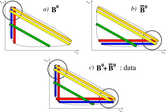
Figure 1: Schematic representation for the stand-alone DP of $a)B^{0}\to K_{S}\pi^{+}\pi^{-}$, $b)\bar{B^{0}}\to K_{S}\pi^{+}\pi^{-}$ and in $c)$ the joint DP obtained from the untagged analysis. Bands are pictorially representing resonances regions, where for simplicity we ignore angular effects in the distribution. Circles are displaying regions of interference. Is the non-overlapping of circles that assures the separation between both amplitudes in the joint fit analysis.

In the Belle $B^{0},\bar{B^{0}}\to K_{S}\pi^{+}\pi^{-}$analysis bellekspipi , the authors fit a untagged sample of $K_{S}\pi\pi$, using as total amplitude the sum $|A(x,y)|^{2}+|A(y,x)|^{2}$. The amplitudes have same parameters of magnitude and phase, assuming no CP violation and differing only by a Dalitz variable exchange. Using the joint fit technique, it’s possible to extract different parameters to both decays and measure experimentally CP violation, giving one step ahead in the technical difficulty existent so far.

IV Feasibility Study

To investigate the feasibility and the error dimension in the joint analysis, we generated and fitted 100 Monte Carlo experiments of 100K $B^{0},\bar{B^{0}}\to K_{S}\pi^{+}\pi^{-}$events (the expected number for one year of data taking in LHCb lhcb ). All resonances are described by Breit-Wigner distributions and the total amplitude is given by (6). The parameters used in the generation were inspired in the observed parameters by BaBark2pi ; bellek2pi . The Dalitz plot distribution for one generated experiment of 100K events is displayed in figure 2, where the small contribution of the resonance $\chi_{c0}$ can be seen.

Figure 2: $B^{0}$, $\bar{B}^{0}\to K_{s}\pi^{+}\pi^{-}$ events distribution from fast MC generated with table 2 parameters.

In table 2, column input, we show the generated magnitudes and phases to each resonance of $B^{0}$ and $\bar{B^{0}}$. The extracted parameters by the joint fit are shown in the last column, where the displayed values are the central values of the gaussian distributions of the 100 experiments and the errors are the width of the same gaussian distribution. One can note that the extracted quantities are in agreement with the generated ones and with small errors, stating the feasibility of the joint fit method.

decay	$B^{0}/\bar{B}^{0}$	input	fit 100K events
$\chi_{c}K_{s}$	$a_{0}/\bar{a}_{0}$	0.30/0.30	fixed/$(0.30\pm 0.03)$
	$\delta_{0}/\bar{\delta}_{0}$	3.78/3.78	fixed/fixed
$K^{*}(890)\pi$	$a_{1}/\bar{a}_{1}$	1.17/1.30	$1.17\pm 0.06$ /$(1.30\pm 0.01)$
	$\delta_{1}/\bar{\delta}_{1}$	0.40/5.98	$(0.41\pm 0.08)$/$(5.99\pm 0.07)$
$K_{0}^{*}(1430)\pi$	$a_{2}/\bar{a}_{2}$	2.45/2.72	$(2.45\pm 0.11)$/$(2.72\pm 0.13)$
	$\delta_{2}/\bar{\delta}_{2}$	0.375/6.00	$(0.39\pm 0.08)$/$(6.00\pm 0.06)$
$\rho^{0}K_{s}$	$a_{3}/\bar{a}_{3}$	0.60/0.60	$(0.60\pm 0.04)$/$(0.60\pm 0.04)$
	$\delta_{3}/\bar{\delta}_{3}$	1.20/1.20	$(1.22\pm 0.09)$/$(1.20\pm 0.07)$
$f_{0}K_{s}$	$a_{4}/\bar{a}_{4}$	1.03/1.03	$(1.02\pm 0.06)$/$(1.04\pm 0.05)$
	$\delta_{4}/\bar{\delta}_{4}$	2.30/2.30	$(2.30\pm 0.07)$/$(2.30\pm 0.08)$

$N^{0}(B^{0}\to K_{s}\pi^{+}\pi^{-})/N^{0}(\bar{B}^{0}\to K_{s}\pi^{+}\pi^{-})$ = 0.84 $\pm$ 0.12

Table 2: Monte Carlo simulation for $B^{0}$, $\bar{B}^{0}\to K_{s}\pi^{+}\pi^{-}$ decay. We generated sample with the the parameters $a_{i}$ and $\delta_{i}$ for $B^{0}$ and $\bar{a}_{i}$ and $\bar{\delta}_{i}$ for $\bar{B}^{0}$. The third column display the fit results with one hundred samples for each 100K events. The last line is the ratio between $B^{0},\bar{B}^{0}\to K_{s}\pi^{+}\pi^{-}$ number of events.

One important issue concerning the $\gamma$ extraction, is the size of the ratio $r=a_{T}/a_{P}$ and the phase difference $\theta=\delta_{T}-\delta_{P}$ from the tree and penguin amplitudes of the $K^{*}$ resonance. The theoretical knowledge of these quantities is model dependent. Some groups using factorization approach neubert , arrive to large $r$ and small $\theta$. On the other hand, non-factorisable approach for pseudoscalar-pseudoscalar $B$ decay buras , presents an opposite scenario, with small $r$ and large $\theta$. The joint fit applied to the real data, will be able to define which theoretical approach is more adequate, since it is possible to measure the parameters under discussion. To our study, we choose $r=0.45$ and generate the experiments with $\gamma=69^{\circ}$.

If in the unconstrained analysis, the three hypothesis prove to be correct, we can assume that the $K^{*}$ resonances parameters from $B^{0}$ and $\bar{B^{0}}$ are given by the following tree and penguin sum:

$$a\,e^{i\,\delta}=a_{P}\,e^{i\,\delta_{P}}+a_{T}\,e^{i\,\theta^{+}},$$

$$\bar{a}\,e^{i\,\bar{\delta}}=a_{P}\,e^{i\,\delta_{P}}+a_{T}\,e^{i\,\theta^{-}}.$$ (7)

In this case, we can use the scheme (1) to extract $\gamma$ using a constrained fit, where the penguin amplitude is fixed and the tree parameters $a_{T}$ and $\theta^{\pm}$ are directly extracted from $K^{*}$. Using the parameters from table 2, we measure $\gamma=69^{\circ}\pm 5^{\circ}$.

V Conclusion

We presented a method to extract the CKM $\gamma$ angle using a combined Dalitz plot analysis from $B^{\pm}\to K^{\pm}\pi^{+}\pi^{-}$ and $B^{0},\bar{B}^{0}\to K_{s}\pi^{+}\pi^{-}$. This approach use three basic hypothesis that can be tested before one proceeds to the constrained fit. For measuring the $B$ neutral parameters, we use a new technique of joint fit that allow us to extract in an independent way the amplitudes from two summed surfaces in a joint sample of $B^{0}+\bar{B}^{0}$ untagged events. We carried a fast MC study to estimate the errors associated to the joint fit technique. Assuming a relatively low statistics for the anchor resonance $\chi_{c0}$ we obtained $\gamma$ with a $5^{\circ}$ error.

During the analysis we can measure CP violation by counting the number of events from $B^{0}$ and $\bar{B^{0}}$, information extracted in the joint fit, or exploring Dalitz symmetries as discussed in burdman . We can also measure the ratio and phase difference from tree and penguin amplitudes of the $K^{*}$ resonance, defining which theoretical approach, factorisable or non-factorisable is more adequate.

The method presented here is competitive with the other approaches to determine the CKM $\gamma$ angle schneider and needs the high statistics expected for the LHCb experiment, due to the small contribution of the reference channel $B\to\chi^{0}K$. However, in the case that the $f_{0}(980)$ resonance is dominated by the $s\bar{s}$ component bnn , or even if the ratio between the tree and penguin is negligible f0 , the $B\to f_{0}(980)K$ amplitude could take place of the charmonium as a reference channel in the analysis.

References

- (1) BaBar Collaboration, B. Aubert et al., Phys. Rev. Lett. 94, 161803 (2005), hep-ex/0408127.
- (2) Belle Collaboration, K. Abe et al, hep-ex/0507037.
- (3) D. Atwood, I. Dunietz, A. Soni, Phys. Rev. Lett. 78, 3257 (1997).
- (4) M. Gronau, D. London, Phys. Lett. B 253, 483 (1991) ; M. Gronau, D. London, Phys. Lett. B 265, 172 (1991).
- (5) A. Giri, Yu. Grossman, A. Soffer, J. Zuppan, Phys. Rev. D 68, 054018 (2003).
- (6) O. Schneider, talk at the ” Flavor in the era of the LHC” workshop, CERN, November 2005, http://cern.ch/flavlhc and, J. Rademacker, talk at the ”Physics at the LHC” workshop, Krakow, July 2006, http://indico.cern.ch/conferenceDisplay.py?confId=a058062.
- (7) I. Bediaga, R. E. Blanco, C. Göbel and R. Méndez-Galain, Phys. Rev. Lett. 81 4067 (1998).
- (8) BaBar Collaboration, B. Aubert et al., hep-ex/0507004.
- (9) Belle Collaboration, A. Garmash et al., Phys. Rev. Lett. 96 251803 (2006), hep-ex/0512066.
- (10) M. Ciuchini, M. Pierini, L.Silvestrini, hep-ph/06010233.
- (11) M. Gronau, D. Pirjol, A. Soni, J. Zupan, hep-ph/0608243.
- (12) I. Bediaga, G. Guerrer, J. Miranda, hep-ph/0608268.
- (13) LHCb Collaboration, Reoptimized detector design and performance report, CERN-LHCC/2003-030.
- (14) Belle collaboration, K. Abe et al., hep-ex/0610081.
- (15) Belle Collaboration, R. Kumar et al., hep-ex/0607008.
- (16) C. W. Chiang et. al., Phys. Rev. D69, 034001 (2004).
- (17) M. Beneke, M. Neubert, Nucl. Phys., B675, 333 (2003).
- (18) G. Burdman and J.F. Donoghue, Phys. Rev. 45 187 (1992)
- (19) S. Gardner, J.Tandean, Phys.Rev. D69, 034011 (2004).
- (20) S. Barsuk for LHCb Collaboration, Nucl. Phys. B, Proc. Suppl. 156, 93 (2006).
- (21) M. Beneke and M.Neubert, Nucl. Phys, B675, 333 (2003).
- (22) A. J. Buras et al., Phys.Rev.Lett.92:101804 (2004).
- (23) I. Bediaga, F.S. Navarra and M, Nielsen Phys. Lett. 579 B, 59 (2004).
- (24) H. Cheng and K. Yang, Phys.Rev.D71:054020, 2005 and A.K. Giri, B. Mawlong and R. Mohanta, hep-ph/0608088.