1 Introduction

Among the possible extensions of the Standard Model (SM), those where the $SU(3)_{C}\times SU(2)_{W}\times U(1)_{Y}$ gauge group is enlarged by a number of extra $U(1)$ symmetries are quite attractive for being modest enough departures from the SM so that they are computationally tractable, but at the same time predictive enough so that they are interesting and even perhaps testable at the LHC. Of particular popularity among these have been models where at least one of the extra $U(1)$’s is ”anomalous”, that is, some of the fermion triangle loops with gauge boson external legs are non-vanishing. The existence of this possibility was noticed in the context of the (compactified to four dimensions) heterotic superstring where the stability of the supersymmetric vacuum [1] can trigger in the four-dimensional low energy effective action a non-vanishing Fayet-Iliopoulos term proportional to the gravitational anomaly, i.e. proportional to the anomalous trace of the corresponding $U(1)$. The mechanism was recognized to be the low energy manifestation of the Green-Schwarz anomaly (GS) cancellation mechanism of string theory. Most of the consequent developments were concentrated around exploiting this idea in conjunction with supersymmetry and the Froggatt-Nielsen mechanism [2] in order to explain the mass hierarchies in the Yukawa sector of the SM [3], supersymmetry breaking [4], inflation [5] and axion physics [6], in all of which the presence of the anomalous $U(1)$ is a crucial ingredient. In the context of theories with extra dimensions the analysis of anomaly localization and of anomaly inflow has also been at the center of interesting developments [7], [8]. The recent explosion of string model building, in particular in the context of orientifold constructions and intersecting branes [10, 11] but also in the context of the heterotic string [12], have enhanced even more the interest in anomalous $U(1)$ models. There are a few universal characteristics that these vacua seem to possess. One is the presence of $U(1)$ gauge symmetries that do not appear in the SM [13, 14]. In realistic four dimensional heterotic string vacua the SM gauge group comes as a subgroup of the ten-dimensional $SO(32)$ or $E_{8}\times E_{8}$ symmetry [15], and in practice there is at least one anomalous $U(1)$ factor that appears at low energies, tied to the SM sector in a particular way, which we will summarize next. For simplicity and reasons of tractability we concentrate on the simplest non-trivial case of a model with gauge group $SU(3)_{C}\times SU(2)_{W}\times U(1)_{Y}\times U(1)_{B}$ where $Y$ is hypercharge and $B$ is the anomalous gauge boson and with the fermion spectrum that of the SM. The mass term for the anomalous $U(1)_{B}$ appears through a Stückelberg coupling [14, 16, 17] and the cancellation of its anomalies is due to four dimensional axionic and Chern-Simons terms (in the open string context see the recent works [14, 18, 19, 20]).

Despite of all this theoretical insight both from the top-down and bottom-up approaches, the question that remains open is how to make concrete contact with experiment. However, as mentioned above, in models with anomalous $U(1)$’s one should quite generally expect the presence of a physical axion-like field $\chi$ and in fact in any decay that involves a non-vanishing fermion triangle like the decay $Z^{*},Z^{{}^{\prime}*}\longrightarrow\gamma\gamma$, $Z,Z^{\prime}\longrightarrow Z\gamma$ etc., one should be able to see traces of the anomalous structure [19, 20, 22, 23]. In this paper we will mostly concentrate on the gauge boson decays which, even though hard to measure, contain clear differences with respect to the SM - as is the case of the $Z^{*}\longrightarrow\gamma\gamma$ decay - and in addition with respect to anomaly free $U(1)$ extensions - like the $Z^{{}^{\prime}*}\longrightarrow\gamma\gamma$ decay - for example.

In [19] a theory which extends the SM with this minimal structure (for essentially an arbitrary number of extra $U(1)$ factors) was called ”Minimal Low Scale Orientifold Model” or MLSOM for short, because in orientifold constructions one typically finds multiple anomalous $U(1)$’s. Here, even though we discuss the case of a single anomalous $U(1)$ which could also originate from heterotic vacua or some field theory extension of the SM, we will keep on using the same terminology keeping in mind that the results can apply to more general cases. We finally mention that other similar constructions with emphasis on other phenomenological signatures of such models have appeared before in [18, 24, 26, 25]. A perturbative study of the renormalization of these types of models is in [27]. Other features of these models, in view of the recent activity connected to the claimed PVLAS result [28], have been discussed in [23].

Our work is organized as follows. In the first sections we will specialize the analysis of [19] to the case of an extension of the SM that contains one additional anomalous abelian $U(1)$, with an abelian structure of the form $U(1)_{Y}\times U(1)_{B}$, that we will analyze in depth. We will determine the structure of the entire lagrangean and fix the counterterms in the 1-loop anomalous effective action which are necessary to restore the gauge invariance of the model at quantum level. The analysis that we provide is the generalization of what is discussed in [23] that was devoted primarily to the analysis of anomalous abelian models and to the perturbative organization of the corresponding effective action. After determining the axion lagrangian and after discussing Higgs-axion mixing in this extension of the SM, we will focus our attention on an analysis of the contributions to a simple process $(Z\to\gamma\gamma)$. Our analysis, in this case, aims to provide an example of how the new contributions included in the effective action - in the form of one loop counterterms that restore unitarity of the effective action - modify the perturbative structure of the process. A detailed phenomenological analysis is beyond the scope of this work, since it requires, to be practically useful for searches at the LHC, a very accurate determination of the QCD and electroweak background around the Z/Z’ resonance. We hope to return to a complete analysis of 3-linear gauge interactions in this class of models in the near future.

2 Effective models at low energy: the $SU(3)_{C}\times SU(2)_{W}\times U(1)_{Y}\times U(1)_{B}$ case

We start by briefly recalling the main features of the MLSOM starting from the expression of the lagrangean which is given by

$${\cal L}\;= - \frac{1}{2}Tr\;[F^{G}_{\mu\nu}F^{G\mu\nu}]-\frac{1}{2}Tr[\;F^{W}_{\mu\nu}F^{W\mu\nu}]-\frac{1}{4}F^{B}_{\mu\nu}F^{B\mu\nu}-\frac{1}{4}F^{Y}_{\mu\nu}F^{Y\mu\nu}$$ (1)

$$+ |(\partial_{\mu}+ig_{2}\frac{\tau^{j}}{2}W_{\mu}^{j}+ig_{Y}q^{Y}_{u}A_{\mu}^{Y}+ig_{B}\frac{q^{B}_{u}}{2}B_{\mu})H_{u}|^{2}$$

$$+ |(\partial_{\mu}+ig_{2}\frac{\tau^{j}}{2}W_{\mu}^{j}+ig_{Y}q^{Y}_{d}A_{\mu}^{Y}+ig_{B}\frac{q^{B}_{d}}{2}B_{\mu})H_{d}|^{2}$$

$$+ \overline{Q}_{Li}\,i\gamma^{\mu}\left(\partial_{\mu}+ig_{3}\frac{\lambda^{a}}{2}G^{a}_{\mu}+ig_{2}\frac{\tau^{j}}{2}W^{j}_{\mu}+ig_{Y}q^{(Q_{L})}_{Y}A^{Y}_{\mu}+ig_{B}q^{(Q_{L})}_{B}B_{\mu}\right)Q_{Li}$$

$$+ \overline{u}_{Ri}\,i\gamma^{\mu}\left(\partial_{\mu}+ig_{Y}q^{(u_{R})}_{Y}A^{Y}_{\mu}+ig_{B}q^{(u_{R})}_{B}B_{\mu}\right){u}_{Ri}+\overline{d}_{Ri}\,i\gamma^{\mu}\left(\partial_{\mu}+ig_{Y}q^{(d_{R})}_{Y}A^{Y}_{\mu}+ig_{B}q^{(d_{R})}_{B}B_{\mu}\right){d}_{Ri}$$

$$+ \overline{L}_{i}\,i\gamma^{\mu}\left(\partial_{\mu}+ig_{2}\frac{\tau^{j}}{2}W^{j}_{\mu}+ig_{Y}q^{(L)}_{Y}A^{Y}_{\mu}+ig_{B}q^{(L)}_{B}B_{\mu}\right)L_{i}$$

$$+ \overline{e}_{Ri}\,i\gamma^{\mu}\left(\partial_{\mu}+ig_{Y}q^{(e_{R})}_{Y}A^{Y}_{\mu}+ig_{B}q^{(e_{R})}_{B}B_{\mu}\right){e}_{Ri}+\overline{\nu}_{Ri}\,i\gamma^{\mu}\left(\partial_{\mu}+ig_{Y}q^{(\nu_{R})}_{Y}A^{Y}_{\mu}+ig_{B}q^{(\nu_{R})}_{B}B_{\mu}\right){\nu}_{Ri}$$

$$- \Gamma^{d}\,\overline{Q}_{L}H_{d}d_{R}-\Gamma^{u}\,\overline{Q}_{L}(i\sigma_{2}H^{*}_{u})u_{R}+c.c.$$

$$- \Gamma^{e}\,\overline{L}H_{d}{e}_{R}-\Gamma^{\nu}\,\overline{L}(i\sigma_{2}H^{*}_{u})\nu_{R}+c.c.$$

$$+ \frac{1}{2}(\partial_{\mu}b+M_{1}B_{\mu})^{2}$$

$$+ \frac{C_{BB}}{M}bF_{B}\wedge F_{B}+\frac{C_{YY}}{M}bF_{Y}\wedge F_{Y}+\frac{C_{YB}}{M}bF_{Y}\wedge F_{B}$$

$$+ \frac{F}{M}bTr[F^{W}\wedge F^{W}]+\frac{D}{M}bTr[F^{G}\wedge F^{G}]$$

$$+ d_{1}BY\wedge F_{Y}+d_{2}YB\wedge F_{B}+c_{1}\epsilon^{\mu\nu\rho\sigma}B_{\mu}C^{SU(2)}_{\nu\rho\sigma}+c_{2}\epsilon^{\mu\nu\rho\sigma}B_{\mu}C^{SU(3)}_{\nu\rho\sigma}$$

$$+ V(H_{u},H_{d},b),$$

where we have summed over the $SU(3)$ index $a=1,2,...,8$, over the $SU(2)$ index $j=1,2,3$ and over the fermion index $i=1,2,3$ denoting a given generation. We have denoted with $F^{G}_{\mu\nu}$ the field-strength for the gluons and with $F^{W}_{\mu\nu}$ the field strength of the weak gauge bosons $W_{\mu}$. $F^{Y}_{\mu\nu}$ and $F^{B}_{\mu\nu}$ are the field-strengths related to the abelian hypercharge and the extra abelian gauge boson, B, which has anomalous interactions with a typical generation of the Standard Model. The fermions in eq. (1) are either left-handed or right-handed Dirac spinors $f_{L}$, $f_{R}$ and they fall in the usual $SU(3)_{C}$ and $SU(2)_{W}$ representations of the Standard Model. The additional anomalous $U(1)_{B}$ is accompanied by a shifting Stückelberg axion $b$. The $c_{i}$, $i=1,2$, are the coefficients of the Chern-Simons trilinear interactions [19, 20] and we have also introduced a mass term $M_{1}$ at tree level for the B gauge boson, which is the Stückelberg term. As usual, the hypercharge is anomaly-free and its embedding in the so called “D-brane basis” has been discussed extensively in the previous literature [13, 24, 16]. Most of the features of the orientifold construction are preserved, but we don’t work with the more general multiple $U(1)$ structure since our goal is to analyze as close as possible this model making contact with direct phenomenological applications, although our results and methods can be promptly generalized to more complex situations.

Before moving to the more specific analysis presented in this work, some comments are in order concerning the possible range of validity of effective actions of this type and the relation between the value of the cutoff parameter $\Lambda$ and the Stückelberg mass $M_{1}$. This point has been addressed before in great detail in [21] and we omit any further elaboration, quoting the result. Lagrangeans containing dimension-5 operators in the form of a Wess-Zumino term may have a range of validity constrained by $M_{1}\geq g_{1}g^{2}/(64\pi^{3})a_{n}\Lambda$, where $g_{1}$ is the coupling at the chiral vertex where the anomaly $a_{n}$ is assigned and g is the coupling constant of the other two vector-like currents in a typical AVV diagram. More quantitatively, this bound can be reasonably assumed to be of the order of $10^{5}$ GeV, by a power-counting analysis. Notice that the arguments of [21], though based on the picture of “partial decoupling” of the fermion spectrum, in which the pseudoscalar field is the phase of a heavier Higgs, remain fully valid in this context (see [21] for more details). The actual value of $M_{1}$ is left undetermined, although in the context of string model building there are suggestions to relate them to specific properties of the compactified extra dimensions (see for instance [13, 16]).

3 The effective action of the MLSOM with a single anomalous $U(1)$

Having derived the essential components of the classical lagrangean of the model, now we try to extend our study to the quantum level, determining the anomalous effective action both for the abelian and the non-abelian sectors, fixing the $D$, $F$ and $C$ coefficients in front of the Green-Schwarz terms in eq. 1. Notice that the only anomalous contributions to ${\cal S}_{an}$ in the Y-basis before symmetry breaking come from the triangle diagrams depicted in Fig. 1.

Figure 1: Anomalous triangle diagrams for the MLSOM.

Since hypercharge is anomaly-free, the only relevant non-abelian anomalies to be canceled are those involving one boson $B$ with two $SU(2)_{W}$ bosons, or two $SU(3)_{C}$ bosons, while the abelian anomalies are those containing three $U(1)$ bosons, with the $Y^{3}$ triangle excluded by the hypercharge assignment. These $(BSU(2)SU(2))$ and $(BSU(3)SU(3))$ anomalies must be canceled respectively by Green-Schwarz terms of the kind

$$F\,b\,Tr[F^{W}\wedge F^{W}],\qquad D\,b\,Tr[F^{G}\wedge F^{G}],$$

with $F$ and $D$ to be fixed by the conditions of gauge invariance. In the abelian sector we have to focus on the BBB, BYY and YBB triangles which generate anomalous contributions that need to be canceled, respectively, by the Green-Schwarz terms $C_{BB}\,b\,F^{B}\wedge F^{B}$, $C_{YY}\,b\,F^{Y}\wedge F^{Y}$ and $C_{YB}\,b\,F^{Y}\wedge F^{B}$. Denoting by ${\cal S}_{YM}$ the anomalous effective action involving the classical non-abelian terms plus the non-abelian anomalous diagrams, and with ${\mathcal{S}}_{ab}$ the analogous abelian one, the complete anomalous effective action is given by

$${\mathcal{S}}_{eff} = {\mathcal{S}}_{0}+{\mathcal{S}}_{YM}+{\mathcal{S}}_{ab}$$ (2)

with ${\mathcal{S}}_{0}$ being the classical lagrangean and

$${\mathcal{S}}_{YM} = \int dx\,dy\,dz\left(\frac{1}{2!}T^{\lambda\mu\nu,ij}_{BWW}(z,x,y)B^{\lambda}(z)W^{\mu}_{i}(x)W^{\nu}_{j}(y)+\frac{1}{2!}T^{\lambda\mu\nu,ab}_{BGG}(z,x,y)B^{\lambda}(z)G^{\mu}_{a}(x)G_{b}^{\nu}(y)\right),$$

$${\mathcal{S}}_{ab} = \int dx\,dy\,dz\left(\frac{1}{3!}T^{\lambda\mu\nu}_{BBB}(z,x,y)B^{\lambda}(z)B^{\mu}(x)B^{\nu}(y)+\frac{1}{2!}T^{\lambda\mu\nu}_{BYY}(z,x,y)B^{\lambda}(z){Y}^{\mu}(x){Y}^{\nu}(y)\right.$$ (4)

$$\left.\qquad\qquad\qquad+\frac{1}{2!}T^{\lambda\mu\nu}_{YBB}(z,x,y){Y}^{\lambda}(z)B^{\mu}(x)B^{\nu}(y)\right).$$

The corresponding 3-point functions, for instance, are given by

$$T^{\lambda\mu\nu,\,ij}_{BWW}B^{\lambda}W^{\mu}_{i}W^{\nu}_{j} = \langle 0|T(J^{\lambda,\,f}_{B}J^{\mu,\,f}_{Wi}J^{\nu,\,f}_{Wj})|0\rangle B^{\lambda}W^{\mu}_{i}W^{\nu}_{j}$$ (5)

$$\equiv \langle 0|T(J^{\lambda,\,f_{L}}_{B}J^{\mu,\,f_{L}}_{Wi}J^{\nu,\,f_{L}}_{Wj})|0\rangle B^{\lambda}W^{\mu}_{i}W^{\nu}_{j},$$

and similarly for the others. Here we have defined the chiral currents

$$J^{\lambda,f}_{B}=J^{\lambda,f_{R}}_{B}+J^{\lambda,f_{L}}_{B}=-g_{B}q^{\,fR}_{B}\,\overline{\psi}_{f}\gamma^{\lambda}P_{R}\psi_{f}-g_{B}q^{\,fL}_{B}\,\overline{\psi}_{f}\gamma^{\lambda}P_{L}\psi_{f}.$$ (6)

The non-abelian W current being chiral

$$J^{\mu,f}_{Wi}\equiv J^{\mu,f_{L}}_{Wi}=-g_{2}\overline{\psi}_{f}\gamma^{\mu}\tau^{i}P_{L}\psi_{f},$$ (7)

it forces the other currents in the triangle diagram to be of the same chirality, as shown in Fig. (7).

4 Three gauge boson amplitudes and gauge fixing

Figure 2: Contributions to a three abelian gauge boson amplitude before the removal of the $B-\partial b$ gauge boson- Stückelberg mixing.

4.1 The non-abelian sector before symmetry breaking

Before we get into the discussion of the gauge invariance of the model, it is convenient to elaborate on the cancelations of the spurious s-channel poles coming from the gauge-fixing conditions. These are imposed to remove the $\partial b-B$ mixing- in the effective action. We will perform our analysis in the basis of the interaction eigenstates since in this basis recovering gauge independence is more straightforward, at least before we enforce symmetry breaking via the Higgs mechanism. The procedure that we follow is to gauge fix the B gauge boson in the symmetric phase by removing the $B-\partial b$ mixing (see Fig. 2 (C)), so to derive simple Ward identities involving only fermionic triangle diagrams and contact trilinear interactions with gauge bosons. For this purpose to the Stückelberg term

$$\frac{1}{2}(\partial_{\mu}b+M_{1}B_{\mu})^{2}\\$$

we add the gauge fixing term

$$\mathcal{L}_{gf}=-\frac{1}{2}\mathcal{G}_{B}^{2}$$ (8)

to remove the bilinear mixing, where

$$\mathcal{G}_{B}=\frac{1}{\sqrt{\xi_{B}}}\left(\partial\cdot B-\xi_{B}M_{1}b\right),$$ (9)

with a propagator for the massive B gauge boson separated in a gauge independent part $P_{0}$ and a gauge dependent one $P_{\xi}$:

$$\frac{-\,i}{k^{2}-M_{1}^{2}}\left(g^{\,\lambda\,\lambda^{\prime}}-\frac{k^{\lambda}\,k^{\lambda^{\prime}}}{M_{1}^{2}}\right)+\frac{-\,i}{k^{2}-\xi_{B}\,M_{1}^{2}}\left(\frac{k^{\lambda}k^{\lambda^{\prime}}}{M_{1}^{2}}\right) = P_{0}^{\lambda\,\lambda^{\prime}}+P_{\xi}^{\lambda\,\lambda^{\prime}}.$$ (10)

We will briefly illustrate here how the cancelation of the gauge dependence due to $b$ and $B$ exchanges in the s-channel goes in this (minimally) gauge-fixed theory. In the exact phase we have no mixing between all the $Y,B,W$ gauge bosons and the gauge dependence of the B propagator is canceled by the Stueckelberg axion. In the broken phase things get more involved, but essentially the pattern continues to hold. In that case the Stückelberg scalar has to be rotated into its physical component $\chi$ and the two Goldstones $G_{Z}$ and $G_{Z^{\prime}}$ which are linear combinations of $G^{0}_{1}$ and $G^{0}_{2}$. The cancelation of the spurious s-channel poles takes place, in this case, via the combined exchange of the $Z$ propagator and of the corresponding Goldstone mode $G_{Z}$. Naturally the GS interaction will be essential for this to happen.

For the moment we simply work in the exact symmetry phase and in the basis of the interaction eigenstates. We gauge fix the action to remove the $B-\partial b$ mixing, but for the rest we set the vev of the scalars to zero. For definiteness let’s consider the process $WW\rightarrow WW$ mediated by a B boson as shown in Fig. 3. We denote by a bold-faced V the $BWW$ vertex, constructed so to have gauge invariance on the W-lines. This vertex, as we are going to discuss next, requires a generalized CS counterterm to have such a property on the W lines. Gauge invariance on the B line, instead, which is clearly necessary to remove the gauge dependence in the gauge fixed action, is obtained at a diagrammatical level by the the axion exchange (Fig. 3).

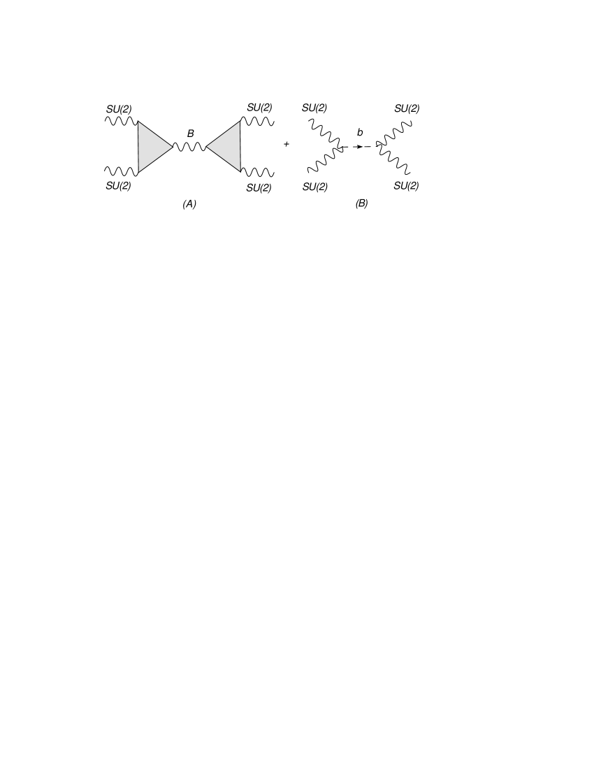
Figure 3: Unitarity check in SU(2) sector for the MLSOM.

The expressions of the two diagrams are

$$A_{\xi}+B_{\xi} = \frac{-i}{k^{2}-\xi_{B}M^{2}_{1}}\frac{1}{M^{2}_{1}}\Big{(}k^{\lambda}{\bf V}^{\lambda\mu\nu}_{BWW}(-k_{1},-k_{2})\Big{)}\left(k^{\lambda^{\prime}}{\bf V}^{\lambda^{\prime}\mu^{\prime}\nu^{\prime}}_{BWW}(k_{1},k_{2})\right)\left(g_{B}g^{\,2}_{2}D^{(L)}_{B}\right)^{2}$$ (11)

$$+\,4\times\left(\frac{4F}{M}\right)^{2}\left(\frac{i}{k^{2}-\xi_{B}M^{2}_{1}}\right)\varepsilon^{\mu\nu\alpha\beta}k^{\alpha}_{1}k^{\beta}_{2}\,\varepsilon^{\mu^{\prime}\nu^{\prime}\alpha^{\prime}\beta^{\prime}}k^{\alpha^{\prime}}_{1}k^{\beta^{\prime}}_{2}.$$

Using the equations for the anomalies and the correct value for the Green-Schwarz coefficient F given in eq. (61) (and that we will determine in the next section), we obtain

$$A_{\xi}+B_{\xi} = \frac{-i}{k^{2}-\xi_{B}M^{2}_{1}}\frac{1}{M^{2}_{1}}\Big{(}-4a_{n}\varepsilon k_{1}k_{2}\Big{)}\Big{(}4a_{n}\varepsilon^{\prime}k^{\prime}_{1}k^{\prime}_{2}\Big{)}\left(g_{B}g^{2}_{2}D^{(L)}_{B}\right)^{2}$$ (12)

$$+\frac{64}{M^{2}}\frac{M^{2}}{M^{2}_{1}}\left(ig_{B}g^{2}_{2}\frac{a_{n}}{2}D^{(L)}_{B}\right)^{2}\left(\frac{i}{k^{2}-\xi_{B}M^{2}_{1}}\right)\varepsilon k_{1}k_{2}\varepsilon^{\prime}k^{\prime}_{1}k^{\prime}_{2}$$

so that the cancelation is easily satisfied. The treatment of the $SU(3)$ sector is similar and we omit it.

4.2 The abelian sector before symmetry breaking

In the abelian sector the procedure is similar. For instance, to test the cancelation of the gauge parameter $\xi_{B}$ in a process $BB\rightarrow BB$ mediated by a B gauge boson we sum the two gauge dependent contributions coming from the diagrams in Fig. 4 (we consider only the gauge dependent part of the s-channel exchange diagrams)

Figure 4: Unitarity check in abelian sector for the MLSOM.

$$A_{\xi}+B_{\xi} = \frac{-i}{k^{2}-\xi_{B}M^{2}_{1}}\frac{1}{M^{2}_{1}}\Big{(}4\,k^{\lambda}{\Delta}^{\lambda\mu\nu}_{\bf AAA}(-k_{1},-k_{2})\Big{)}\left(4\,k^{\lambda^{\prime}}{\Delta}^{\lambda^{\prime}\mu^{\prime}\nu^{\prime}}_{\bf AAA}(k_{1},k_{2})\right)\left(g^{3}_{B}D_{BBB}\right)^{2}$$ (13)

$$+\,4\times\left(\frac{4}{M}C_{BB}\right)^{2}\frac{i}{k^{2}-\xi_{B}M^{2}_{1}}\,\varepsilon k_{1}k_{2}\,\varepsilon^{\prime}k^{\prime}_{1}k^{\prime}_{2},$$

and cancelation of the gauge dependences implies that the following identity must hold

$$\frac{16}{M^{2}_{1}}\left(\frac{a_{n}}{3}\right)^{2}\left(g^{\,3}_{B}D_{BBB}\right)^{2}+4\times\left(\frac{4}{M}C_{BB}\right)^{2}=0,$$ (14)

which can be easily shown to be true after substituting the value of the GS coefficient given in relation (76).

In Fig. (5) we have depicted the anomalous triangle diagram BYY (A) which has to be canceled by the Green-Schwarz term $\frac{C_{YY}}{M}bF^{Y}\wedge F^{Y}$, that generates diagram (B). In this case the two diagrams give

Figure 5: Unitarity check in abelian sector for the MLSOM.

$$A_{\xi}+B_{\xi} = \frac{-i}{k^{2}-\xi_{B}M^{2}_{1}}\frac{1}{M^{2}_{1}}\Big{(}k^{\lambda}{\bf V}^{\lambda\mu\nu}_{BYY}(-k_{1},-k_{2})\Big{)}\left(k^{\lambda^{\prime}}{\bf V}^{\lambda^{\prime}\mu^{\prime}\nu^{\prime}}_{BYY}(k_{1},k_{2})\right)\left(g_{B}g^{2}_{Y}D_{BYY}\right)^{2}$$ (15)

$$+\,4\times\left(\frac{4}{M}C_{YY}\right)^{2}\frac{i}{k^{2}-\xi_{B}M^{2}_{1}}\,\varepsilon k_{1}k_{2}\,\varepsilon^{\prime}k^{\prime}_{1}k^{\prime}_{2}.$$

The condition of unitarity of the amplitude requires the validity of the identity

$$\frac{16}{M^{2}_{1}}\,{a_{n}}^{2}\left(g_{B}g^{\,2}_{Y}D_{BYY}\right)^{2}+4\times\left(\frac{4}{M}C_{YY}\right)^{2}=0,$$ (16)

which can be easily checked substituting the value of the GS coefficient $C_{YY}$ given in relation (77). We will derive the expressions of these coefficients and the factors of all the other counterterms in the next section. The gauge dependences appearing in the diagrams shown in Fig. 6 are analyzed in a similar way and we omit repeating the previous steps, but it should be obvious by now how the perturbative expansion is organized in terms of tree-level vertices and 1-loop counterterms, and how gauge invariance is checked at higher orders when the propagators of the B gauge boson and of the axion b are both present. Notice that in the exact phase the axion $b$ is not coupled to the fermions and the pattern of cancelations to ensure gauge independence, in this specific case, is simplified.

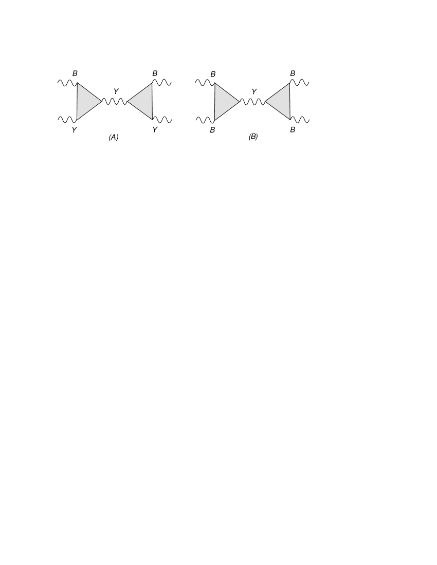
Figure 6: Unitarity check in abelian sector for the MLSOM.

At this point we pause to make some comments. The mixed anomalies analyzed above involve a non-anomalous abelian gauge boson and the remaining gauge interactions (abelian/non-abelian). To be specific, in our model with a single non-anomalous $U(1)$, which is the hypercharge $U(1)_{Y}$ gauge group, these mixed anomalies are those involving triangle diagrams with the $Y$ and $B$ generators or the $B$ accompanied by the non-abelian sector. Consider, for instance, the $BYY$ triangle, which appears in the $YB\rightarrow YB$ amplitude. There are two options that we can follow. Either we require that the corresponding traces of the generators over each generation vanish identically

$$Tr[q^{2}_{Y}q_{B}]=-2\left(-\frac{1}{2}\right)^{2}q^{(L)}_{B}+(-1)^{2}q^{(e_{R})}_{B}+3\left[-2\left(\frac{1}{6}\right)^{2}q^{(Q_{L})}_{B}+\left(\frac{2}{3}\right)^{2}q^{(u_{R})}_{B}+\left(-\frac{1}{3}\right)^{2}q^{(d_{R})}_{B}\right]=0,$$

which can be viewed as a specific condition on the charges of model or, if this is not the case, we require that suitable one-loop counterterms balance the anomalous gauge variation. We are allowed, in other words, to fix the two divergent invariant amplitudes of the triangle diagram so that the corresponding Ward identities for the $BYY$ vertex and similar anomalous vertices are satisfied. This is a condition on the parameterization of the Feynman vertex rather than on the charges and is, in principle, allowed. It is not necessary to have a specific determination of the charges for this to occur, as far as the counterterms are fixed accordingly. For instance, in the abelian sector the diagrams in question are

$$YB\rightarrow YB\,\,\mbox{mediated by Y}\,\, \propto \,\,Tr[q^{2}_{Y}q_{B}]\,\,$$

$$YY\rightarrow YY\mbox{mediated by B}\,\, \propto \,\,Tr[q^{2}_{Y}q_{B}]\,\,$$

$$BB\rightarrow BB\,\,\mbox{mediated by Y}\,\, \propto \,\,Tr[q_{Y}q^{2}_{B}]\,\,$$

$$YB\rightarrow YB\,\,\mbox{mediated by B}\,\, \propto \,\,Tr[q_{Y}q^{2}_{B}].\,\,$$

In the MLSOM these traces are, in general, non vanishing and therefore we need to introduce defining Ward identities to render the effective action anomaly free.

5 Ward Identities, Green-Schwarz and Chern-Simons counterterms in the Stückelberg phase

Having discussed the structure of the theory in the basis of the interaction eigenstates, we come now to identify the coefficients needed to enforce cancelation of the anomalies in the 1-loop effective action. In the basis of the physical gauge bosons we will be dropping, with this choice, a gauge dependent ( $B\partial b$ mixing) term that is vanishing for physical polarizations. At the same time, for exchanges of virtual gauge bosons, the gauge dependence of the corresponding propagators is canceled by the associated Goldstone exchanges.

Starting from the non abelian contributions, the $BWW$ amplitude, we separate the charge/coupling constant dependence of a given diagram from the rest of its parametric structure ${\bf T}$ using, in the $SU(2)$ case, the relations

$$T^{\lambda\mu\nu,ij}_{BWW}B^{\lambda}W^{\mu}_{i}W^{\nu}_{j} = g_{B}g^{\,2}_{2}\sum_{i,j}Tr[\tau_{i}\tau_{j}]\frac{1}{8}Tr[q^{L}_{B}]\,{\bf{T}}^{\,\lambda\mu\nu}B^{\lambda}W^{\mu}_{i}W^{\nu}_{j}$$ (19)

$$= \frac{1}{2}g_{B}g^{\,2}_{2}\sum_{i}\,D^{(L)}_{B}\,{\bf{T}}^{\,\lambda\mu\nu}B^{\lambda}W^{\mu}_{i}W^{\nu}_{i},$$

having defined $D^{(L)}_{B}=\frac{1}{8}Tr[q^{L}_{B}]=-\frac{1}{8}\sum_{f}q^{fL}_{B}$ and ${\bf{T}}^{\lambda\mu\nu}$ is the 3-point function in configuration space, with all the couplings and the charges factored out, symmetrized in $\mu\nu$. Similarly, for the coupling of $B$ to the gluons we obtain

$$T^{\lambda\mu\nu,ab}_{BGG}B^{\lambda}G^{\mu}_{a}G^{\nu}_{b} = g_{B}g^{\,2}_{3}\sum_{a,b}\,Tr[T_{a}T_{b}]\frac{1}{8}Tr[q^{L}_{B}]\,{\bf{T}}^{\,\lambda\mu\nu}B^{\lambda}G^{\mu}_{a}G^{\nu}_{b}$$ (20)

$$= \frac{1}{2}g_{B}g^{\,2}_{3}\sum_{a}D^{(L)}_{B}\,{\bf{T}}^{\,\lambda\mu\nu}B^{\lambda}G^{\mu}_{a}G^{\nu}_{a},$$

while the abelian triangle diagrams are given by

$$T^{\lambda\mu\nu}_{BBB}B^{\lambda}B^{\mu}B^{\nu} = g^{\,3}_{B}\,\frac{1}{8}Tr[q^{\,3}_{B}]\,{\bf T}^{\,\lambda\mu\nu}B^{\lambda}B^{\mu}B^{\nu}=g^{\,3}_{B}\,D_{BBB}\,{\bf{T}}^{\,\lambda\mu\nu}B^{\lambda}B^{\mu}B^{\nu},$$ (21)

$${T}^{\lambda\mu\nu}_{BYY}B^{\lambda}Y^{\mu}Y^{\nu} = g_{B}g^{\,2}_{Y}\,\frac{1}{8}Tr[q_{B}q^{\,2}_{Y}]\,{\bf{T}}^{\,\lambda\mu\nu}B^{\lambda}Y^{\mu}Y^{\nu}$$ (22)

$$= g_{B}g^{\,2}_{Y}\,D_{BYY}\,{\bf{T}}^{\,\lambda\mu\nu}B^{\lambda}Y^{\mu}Y^{\nu},$$

$$T^{\lambda\mu\nu}_{YBB}Y^{\lambda}B^{\mu}B^{\nu} = g_{Y}g^{\,2}_{B}\,\frac{1}{8}Tr[q_{Y}q^{\,2}_{B}]\,{\bf{T}}^{\,\lambda\mu\nu}Y^{\lambda}B^{\mu}B^{\nu}$$ (23)

$$= g_{Y}g^{\,2}_{B}\,D_{YBB}\,{\bf{T}}^{\,\lambda\mu\nu}Y^{\lambda}B^{\mu}B^{\nu},$$

with the following definitions for the traces (see also the discussion in the Appendix)

$$D_{BBB} = \frac{1}{8}Tr[q^{3}_{B}]=\frac{1}{8}\sum_{f}\left[(q^{fR}_{B})^{3}-(q^{fL}_{B})^{3}\right],$$ (24)

$$D_{BYY} = \frac{1}{8}Tr[q_{B}q^{2}_{Y}]=\frac{1}{8}\sum_{f}\left[q^{fR}_{B}(q^{fR}_{Y})^{2}-q^{fL}_{B}(q^{fL}_{Y})^{2}\right],$$ (25)

$$D_{YBB} = \frac{1}{8}Tr[q_{Y}q^{2}_{B}]=\frac{1}{8}\sum_{f}\left[q^{fR}_{Y}(q^{fR}_{B})^{2}-q^{fL}_{Y}(q^{fL}_{B})^{2}\right].$$ (26)

The ${\bf T}$ vertex is given by the usual combination of vector and axial-vector components

$${\bf T}^{\lambda\mu\nu}=T^{\lambda\mu\nu}_{\bf AAA}+T^{\lambda\mu\nu}_{\bf AVV}+T^{\lambda\mu\nu}_{\bf VAV}+T^{\lambda\mu\nu}_{\bf VVA},$$ (27)

and we denote by ${\bf\Delta}(k_{1},k_{2})$ its expression in momentum space

$$(2\pi)^{4}\delta(k-k_{1}-k_{2}){\bf\Delta}^{\lambda\mu\nu}(k_{1},k_{2})=\int dxdydze^{ik_{1}\cdot x+ik_{2}\cdot y-ik\cdot z}\,{\bf{T}}^{\lambda\mu\nu}(z,x,y).$$ (28)

We denote similarly with ${\bf\Delta}_{\bf AVV}^{\lambda\mu\nu},{\bf\Delta}_{\bf VAV}^{\lambda\mu\nu},{\bf\Delta}_{\bf VVA}^{\lambda\mu\nu}$ the momentum space expressions of the corresponding x-space vertices ${\bf T}_{\bf AVV}^{\lambda\mu\nu},{\bf T}_{\bf VVA}^{\lambda\mu\nu},{\bf T}_{\bf VAV}^{\lambda\mu\nu}$ respectively.

Figure 7: All the anomalous electroweak contributions to a triangle diagram in the non-abelian sector in the massless fermion case

As illustrated in Fig. (7) and Fig. (8), the complete structure of ${\bf T}$ is given by

$${\bf\Delta}^{\lambda\mu\nu}(k_{1},k_{2}) = \frac{1}{3}\left[{\Delta}^{\lambda\mu\nu}(-1/2,k_{1},k_{2})+{\Delta}^{\mu\nu\lambda}(-1/2,k_{2},-k)+{\Delta}^{\nu\lambda\mu}(-1/2,-k,k_{1})\right]$$ (29)

$$+{\Delta}^{\lambda\mu\nu}(-1/2,k_{1},k_{2})+{\Delta}^{\mu\nu\lambda}(-1/2,k_{2},-k)+{\Delta}^{\nu\lambda\mu}(-1/2,-k,k_{1})$$

$$= \frac{4}{3}\left[{\Delta}^{\lambda\mu\nu}(-1/2,k_{1},k_{2})+{\Delta}^{\mu\nu\lambda}(-1/2,k_{2},-k)+{\Delta}^{\nu\lambda\mu}(-1/2,-k,k_{1})\right]$$

$$= 4\Delta^{\lambda\mu\nu}_{\bf AAA},$$

where we have used the relation between the ${\bf\Delta}_{\bf AAA}$ (bold-faced) vertex and the usual $\Delta$ vertex, which is of the form ${\bf AVV}$. Notice that

$${\bf\Delta}^{\lambda\mu\nu}_{\bf AVV} = {\Delta}^{\lambda\mu\nu}(-1/2,k_{1},k_{2}),$$

$${\bf\Delta}^{\mu\nu\lambda}_{\bf AVV} = {\Delta}^{\mu\nu\lambda}(-1/2,k_{2},-k),$$

$${\bf\Delta}^{\nu\lambda\mu}_{\bf AVV} = {\Delta}^{\nu\lambda\mu}(-1/2,-k,k_{1}),$$ (30)

are the usual vertices with conserved vector current (CVC) on two lines and the anomaly on a single axial vertex.

The AAA vertex is constructed by symmetrizing the distribution of the anomaly on each of the three chiral currents, which is the content of (29). The same vertex can be obtained from the basic AVV vertex by a suitable shift, with $\beta=1/6$, and then repeating the same procedure on the other indices and external momenta, with a cyclic permutation. We obtain

$$\Delta^{\lambda\mu\nu}_{\bf AAA}(1/6,k_{1},k_{2}) = \Delta^{\lambda\mu\nu}(-1/2,k_{1},k_{2})-\frac{i}{4\pi^{2}}\frac{2}{3}\epsilon^{\lambda\mu\nu\sigma}(k_{1}-k_{2})_{\sigma}$$

and its corresponding anomaly equations are given by

$$k_{\lambda}\Delta^{\lambda\mu\nu}_{\bf AAA}(1/6,k_{1},k_{2}) = \frac{a_{n}}{3}\varepsilon^{\,\mu\nu\alpha\beta}k_{1\alpha}k_{2\beta}$$

$$k_{1\mu}\Delta^{\lambda\mu\nu}_{\bf AAA}(1/6,k_{1},k_{2}) = \frac{a_{n}}{3}\varepsilon^{\,\lambda\nu\alpha\beta}k_{1\alpha}k_{2\beta}$$

$$k_{2\nu}\Delta^{\lambda\mu\nu}_{\bf AAA}(1/6,k_{1},k_{2}) = \frac{a_{n}}{3}\varepsilon^{\,\lambda\mu\alpha\beta}k_{2\alpha}k_{1\beta},$$ (32)

typical of a symmetric distribution of the anomaly.

These identities are obtained from the general shift-relation

$$\Delta^{\lambda\mu\nu}(\beta^{\prime},k_{1},k_{2})=\Delta^{\lambda\mu\nu}(\beta,k_{1},k_{2})+\frac{i}{4\pi^{2}}(\beta-\beta^{\prime})\epsilon^{\lambda\mu\nu\sigma}(k_{1}-k_{2})_{\sigma}.$$ (33)

Vertices with conserved axial currents (CAC) can be related to the symmetric AAA vertex in a similar way

$$\Delta^{\lambda\mu\nu}_{\bf AAA}(+1/6,k_{1},k_{2})=\{\Delta^{\lambda\mu\nu}(+1/2,k_{1},k_{2})\}_{CAC}+\frac{i}{4\pi^{2}}\,\frac{1}{3}\,\epsilon^{\lambda\mu\nu\sigma}(k_{1}-k_{2})_{\sigma}.$$ (34)

At this point we are ready to introduce the complete vertices for this model, which are given by the amplitude (28) with the addition of the corresponding Chern-Simons counterterms, were required. These will be determined later in this section by imposing the conservation of the $SU(2)$, $SU(3)$ and $Y$ gauge currents. Following this definition for all the anomalous vertices, the amplitudes can then be written as

$${\bf{\mathcal{V}}}^{\lambda\mu\nu,\,aa}_{BGG}B^{\lambda}G^{\mu}_{a}G^{\nu}_{a} = \frac{1}{2}g_{B}g^{\,2}_{3}D^{(L)}_{B}{\bf T}^{\lambda\mu\nu}B^{\lambda}G^{\mu}_{a}G^{\nu}_{a}+c_{2}\epsilon^{\mu\nu\rho\sigma}B_{\mu}C^{SU(3)}_{\nu\rho\sigma}$$

$${\bf{\mathcal{V}}}^{\lambda\mu\nu,\,ii}_{BWW}B^{\lambda}W^{\mu}_{i}W^{\nu}_{i} = \frac{1}{2}g_{B}g^{\,2}_{2}D^{(L)}_{B}{\bf T}^{\lambda\mu\nu}B^{\lambda}W^{\mu}_{i}W^{\nu}_{i}+c_{1}\epsilon^{\mu\nu\rho\sigma}B_{\mu}C^{SU(2)}_{\nu\rho\sigma}$$

$${\bf{\mathcal{V}}}^{\lambda\mu\nu}_{BYY}B^{\lambda}Y^{\mu}Y^{\nu} = g_{B}g^{\,2}_{Y}D_{BYY}{\bf T}^{\lambda\mu\nu}B^{\lambda}Y^{\mu}Y^{\nu}+d_{1}BY\wedge F_{Y}$$

$${\bf{\mathcal{V}}}^{\lambda\mu\nu}_{YBB}Y^{\lambda}B^{\mu}B^{\nu} = g_{Y}g^{\,2}_{B}D_{YBB}{\bf T}^{\lambda\mu\nu}Y^{\lambda}B^{\mu}B^{\nu}+d_{2}YB\wedge F_{B},$$

$${\bf{\mathcal{V}}}^{\lambda\mu\nu}_{BBB}B^{\lambda}B^{\mu}B^{\nu} = g^{\,3}_{B}D_{BBB}{\bf T}^{\lambda\mu\nu}B^{\lambda}B^{\mu}B^{\nu}$$

which are the anomalous vertices of the effective action, corrected when necessary by suitable CS interactions in order to conserve all the gauge currents at 1-loop.

Before we proceed with our analysis, which has the goal to determine explicitly the counterterms in each of these vertices, we pause for some practical considerations. It is clear that the scheme that we have followed in order to determine the structure of the vertices of the effective action has been to assign the anomaly only to the chiral vertices and to impose conservation of the vector current. There are regularization schemes in the literature that enforce this principle, the most famous one being dimensional regularization with the t’Hooft Veltman prescription for $\gamma_{5}$ (see also the discussion in part 1). In this scheme the anomaly is equally distributed for vertices of the form AAA and is assigned only to the axial-vector vertex in triangles of the form AVV and similar. Diagrams of the form AAV are zero by Furry’s theorem, being equivalent to VVV.

We could also have proceeded in a different way, for instance by defining each $\mathcal{V}$, for instance ${\mathcal{V}}_{BYY}$, to have an anomaly only on the B vertex and not on the Y vertices, even if Y has both a vector and an axial-vector components at tree level and is, indeed, a chiral current. This implies that at 1-loop the chiral projector has to be moved from the Y to to the B vertex “by hand”, no matter if it appears on the Y current or on the B current, rendering the Y current effectively vector-like at 1 loop. This is also what a CS term does. In both cases we are anyhow bond to define separately the 1-loop vertices as new entities, unrelated to the tree level currents. However, having explicit Chern-Simons counterterms renders the treatment compatible with dimensional regularization in the t’Hooft-Veltman prescription. It is clear, however, that one way or the other, the quantum action is not fixed at classical level since the counterterms are related to quantum effects and the corresponding Ward identities, which force the cancelation of the anomaly to take place in a completely new way respect to the SM case, are indeed defining conditions on the theory.

Having clarified this subtle point, we return to the determination of the gauge invariance conditions for our anomalous vertices.

Under B-gauge transformations we have the following variations (singlet anomalies) of the effective action

$$\frac{1}{2!}\delta_{B}<T_{BWW}BWW>=i\frac{g_{B}g^{\,2}_{2}}{2!}\,\frac{4}{3}a_{n}\,\frac{1}{4}\langle\theta_{B}F^{W}_{i}\wedge F^{W}_{j}\rangle\,Tr[\tau^{i}\tau^{j}]\,D^{(L)}_{B},$$ (36)

$$\frac{1}{2!}\delta_{B}<T_{BGG}BGG>=i\frac{g_{B}g^{\,2}_{3}}{2!}\,\frac{4}{3}a_{n}\,\frac{1}{4}\langle\theta_{B}F^{G}_{a}\wedge F^{G}_{b}\rangle\,Tr[T^{a}T^{b}]\,D^{(L)}_{B},$$ (37)

and with the normalization given by

$$Tr[\tau^{i}\tau^{j}]=\frac{1}{2}\delta^{ij}\qquad Tr[T^{a}T^{b}]=\frac{1}{2}\delta^{ab}$$ (38)

we obtain

$$\frac{1}{2!}\delta_{B}<T_{BSU(2)SU(2)}BWW> = i\frac{g_{B}g^{\,2}_{2}}{2!}\,\frac{a_{n}}{6}\,\langle\theta_{B}F^{W}_{i}\wedge F^{W}_{i}\rangle D^{(L)}_{B},$$ (39)

$$\frac{1}{2!}\delta_{B}<T_{BSU(3)SU(3)}BGG> = i\frac{g_{B}g^{\,2}_{3}}{2!}\,\frac{a_{n}}{6}\,\langle\theta_{B}F^{G}_{a}\wedge F^{G}_{a}\rangle D^{(L)}_{B}.$$ (40)

Note, in particular, that the covariantization of the anomalous contributions requires the entire non-abelian field strengths $F^{W}_{i,\,\mu\nu}$ and $F^{G}_{a,\,\mu\nu}$

$$F^{W}_{i,\,\mu\nu} = \partial_{\mu}W^{i}_{\nu}-\partial_{\nu}W^{i}_{\mu}-g_{2}\varepsilon_{ijk}W^{j}_{\mu}W^{k}_{\nu}=\hat{F}^{W}_{i,\,\mu\nu}-g_{2}\varepsilon_{ijk}W^{j}_{\mu}W^{k}_{\nu}$$ (41)

$$F^{G}_{a,\,\mu\nu} = \partial_{\mu}G^{a}_{\nu}-\partial_{\nu}G^{a}_{\mu}-g_{3}f_{abc}G^{b}_{\mu}G^{c}_{\nu}=\hat{F}^{G}_{a,\,\mu\nu}-g_{3}f_{abc}G^{b}_{\mu}G^{c}_{\nu}.$$ (42)

The covariantization of the right-hand-side (rhs) of the anomaly equations takes place via higher order corrections, involving correlators with more external gauge lines. It is well known, though, that the cancelation of the anomalies in these higher order non-abelian diagrams (in d=4) is only related to the triangle diagram (see [23]).

Under the non-abelian gauge transformations we have the following variations

$$\frac{1}{2!}\delta_{SU(2)}\langle T_{BWW}BWW\rangle = i\frac{g_{B}g^{\,2}_{2}}{2!}\frac{8}{3}a_{n}\frac{1}{4}\langle F^{B}\wedge Tr[\theta\hat{F}^{W}]\rangle D^{(L)}_{B}$$ (43)

$$\frac{1}{2!}\delta_{SU(3)}\langle T_{BGG}BGG\rangle = i\frac{g_{B}g^{\,2}_{3}}{2!}\frac{8}{3}a_{n}\frac{1}{4}\langle F^{B}\wedge Tr[\vartheta\hat{F}^{G}]\rangle D^{(L)}_{B},$$ (44)

where the “hat” field strengths $\hat{F}^{W}$ and $\hat{F}^{G}$ refer to the abelian part of the non-abelian field strengths W and G. Introducing the notation

$$Tr[\theta\hat{F}^{W}] = Tr[\tau^{i}\tau^{j}]\theta_{i}\hat{F}^{W}_{j}=\frac{1}{2}\theta_{i}\hat{F}^{W}_{i}\;\;\,\,\,\,\,\,\,\,i,j=1,2,3$$ (45)

$$Tr[\vartheta\hat{F}^{G}] = Tr[T^{a}T^{b}]\vartheta_{a}\hat{F}^{G}_{b}=\frac{1}{2}\vartheta_{a}\hat{F}^{G}_{a}\,\,\;\;\,\,\,\,\,\,a,b=1,2,..,8$$ (46)

the expressions of the variations become

$$\frac{1}{2!}\delta_{SU(2)}\langle T_{BWW}BWW\rangle = i\frac{g_{B}g^{\,2}_{2}}{2!}\frac{a_{n}}{3}\langle\theta_{i}F^{B}\wedge\hat{F}^{W}_{i}\rangle D^{(L)}_{B}$$ (47)

$$\frac{1}{2!}\delta_{SU(3)}\langle T_{BGG}BGG\rangle = i\frac{g_{B}g^{\,2}_{3}}{2!}\frac{a_{n}}{3}\langle\vartheta_{a}F^{B}\wedge\hat{F}^{G}_{a}\rangle D^{(L)}_{B}.$$ (48)

We have now to introduce the Chern-Simons counterterms for the non-abelian gauge variations

$${\mathcal{S}}^{CS}_{non-ab}={\mathcal{S}}^{CS}_{BWW}+{\mathcal{S}}^{CS}_{BGG}=c_{1}\langle\varepsilon^{\mu\nu\rho\sigma}B_{\mu}C^{SU(2)}_{\nu\rho\sigma}\rangle+c_{2}\langle\varepsilon^{\mu\nu\rho\sigma}B_{\mu}C^{SU(3)}_{\nu\rho\sigma}\rangle,$$ (49)

with the non-abelian CS forms given by

$$C^{SU(2)}_{\mu\nu\rho} = \frac{1}{6}\left[W^{i}_{\mu}\left(F^{W}_{i,\,\nu\rho}+\frac{1}{3}\,g_{2}\,\varepsilon^{ijk}W^{j}_{\nu}W^{k}_{\rho}\right)+cyclic\right],$$ (50)

$$C^{SU(3)}_{\mu\nu\rho} = \frac{1}{6}\left[G^{a}_{\mu}\left(F^{G}_{a,\,\nu\rho}+\frac{1}{3}\,g_{3}\,f^{abc}G^{b}_{\nu}G^{c}_{\rho}\right)+cyclic\right],$$ (51)

whose variations under non-abelian gauge transformations are

$$\delta_{SU(2)}C^{SU(2)}_{\mu\nu\rho} = \frac{1}{6}\left[\partial_{\mu}\theta^{i}\,(\hat{F}^{W}_{i,\,\nu\rho})+cyclic\right],$$ (52)

$$\delta_{SU(3)}C^{SU(3)}_{\mu\nu\rho} = \frac{1}{6}\left[\partial_{\mu}\vartheta^{a}\,(\hat{F}^{G}_{a,\,\nu\rho})+cyclic\right].$$ (53)

The variations of the Chern-Simons counterterms then become

$$\delta_{SU(2)}{\mathcal{S}}^{CS}_{BWW} = \frac{c_{1}}{2}\,\frac{1}{2}\langle\theta^{i}F^{B}\wedge\hat{F}^{W}_{i}\rangle$$ (54)

$$\delta_{SU(3)}{\mathcal{S}}^{CS}_{BGG} = \frac{c_{2}}{2}\,\frac{1}{2}\langle\vartheta^{a}F^{B}\wedge\hat{F}^{G}_{a}\rangle,$$ (55)

and we can choose the coefficients in front of the CS counterterms to obtain anomaly cancelations for the non-abelian contributions

$$c_{1}=-ig_{B}g^{\,2}_{2}\frac{2}{3}a_{n}D^{(L)}_{B}\qquad c_{2}=-ig_{B}g^{\,2}_{3}\frac{2}{3}a_{n}D^{(L)}_{B}.$$ (56)

The variations under B-gauge transformations for the related CS counterterms are then given by

$$\delta_{B}{\mathcal{S}}^{CS}_{BWW} = -\frac{c_{1}}{2}\,\frac{1}{2}\langle\theta_{B}F^{W}_{i}\wedge F^{W}_{i}\rangle$$ (57)

$$\delta_{B}{\mathcal{S}}^{CS}_{BGG} = -\frac{c_{2}}{2}\,\frac{1}{2}\langle\theta_{B}F^{G}_{a}\wedge F^{G}_{a}\rangle,$$ (58)

where the coefficients $c_{i}$ are given in (56). The variations under the B-gauge transformations for the $SU(2)$ and $SU(3)$ Green-Schwarz counterterms are respectively given by

$$\frac{F}{M}\,\delta_{B}\langle\,b\,Tr[F^{W}\wedge F^{W}]\,\rangle = -F\frac{M_{1}}{M}\frac{1}{2}\langle\theta_{B}F^{W}_{i}\wedge F^{W}_{i}\rangle,$$ (59)

$$\frac{D}{M}\,\delta_{B}\langle\,b\,Tr[F^{G}\wedge F^{G}]\,\rangle = -D\frac{M_{1}}{M}\frac{1}{2}\langle\theta_{B}F^{G}_{a}\wedge F^{G}_{a}\rangle,$$ (60)

and the cancelation of the anomalous contributions coming from the B-gauge transformations determines $F$ and $D$ as

$$F=\frac{M}{M_{1}}ig_{B}g^{\,2}_{2}\,\frac{a_{n}}{2}\,D^{(L)}_{B},\qquad D=\frac{M}{M_{1}}ig_{B}g^{\,2}_{3}\,\frac{a_{n}}{2}\,D^{(L)}_{B}.$$ (61)

Figure 8: All the anomalous contributions to a triangle diagram in the abelian sector for generic vector-axial vector trilinear interactions in the massless fermion case

There are some comments to be made concerning the generalized CS terms responsible for the cancelation of the mixed anomalies. These terms, in momentum space, generate standard trilinear CS interactions, whose momentum structure is exactly the same as that due to the abelian ones (see the appendix of part 1 for more details), plus additional quadrilinear (contact) gauge interactions. These will be neglected in our analysis since we will be focusing in the next sections on the characterization of neutral tri-linear interactions. In processes such as $Z\to\gamma\gamma\gamma$ they re-distribute the anomaly appropriately in higher point functions.

For the abelian part ${\mathcal{S}}_{ab}$ of the effective action we first focus on gauge variations on B, obtaining

$$\frac{1}{3!}\delta_{B}\langle T^{\lambda\mu\nu}_{BBB}B^{\lambda}(z)B^{\mu}(x)B^{\nu}(y)\rangle=i\frac{g^{\,3}_{B}}{3!}\frac{4}{3}a_{n}\frac{3}{4}\langle F^{B}\wedge F^{B}\theta_{B}\rangle\,D_{BBB},$$ (62)

$$\frac{1}{2!}\delta_{B}\langle T^{\lambda\mu\nu}_{BYY}B^{\lambda}(z)Y^{\mu}(x)Y^{\nu}(y)\rangle=i\frac{g_{B}g^{2}_{Y}}{2!}\frac{4}{3}a_{n}\frac{1}{4}\langle F^{Y}\wedge F^{Y}\theta_{B}\rangle\,D_{BYY},$$ (63)

$$\frac{1}{2!}\delta_{B}\langle T^{\lambda\mu\nu}_{YBB}Y^{\lambda}(z)B^{\mu}(x)B^{\nu}(y)\rangle=i\frac{g_{Y}g^{2}_{B}}{2!}\frac{4}{3}a_{n}\frac{2}{4}\langle F^{Y}\wedge F^{B}\theta_{B}\rangle\,D_{YBB},$$ (64)

and variations for $Y$ that give

$$\frac{1}{2!}\delta_{Y}\langle T^{\lambda\mu\nu}_{BYY}B^{\lambda}(z)Y^{\mu}(x)Y^{\nu}(y)\rangle=i\frac{g_{B}g^{2}_{Y}}{2!}\frac{4}{3}a_{n}\frac{2}{4}\langle F^{Y}\wedge F^{B}\theta_{Y}\rangle\,D_{BYY},$$ (65)

$$\frac{1}{2!}\delta_{Y}\langle T^{\lambda\mu\nu}_{YBB}Y^{\lambda}(z)B^{\mu}(x)B^{\nu}(y)\rangle=i\frac{g_{Y}g^{2}_{B}}{2!}\frac{4}{3}a_{n}\frac{1}{4}\langle F^{B}\wedge F^{B}\theta_{Y}\rangle\,D_{YBB}.$$ (66)

Also in this case we introduce the corresponding abelian Chern-Simons counterterms

$${\mathcal{S}}^{CS}_{ab}={\mathcal{S}}^{CS}_{BYY}+{\mathcal{S}}^{CS}_{YBB}=d_{1}\langle BY\wedge F_{Y}\rangle+d_{2}\langle YB\wedge F_{B}\rangle$$ (67)

whose variations are given by

$$\delta_{Y}{\mathcal{S}}^{CS}_{BYY} = \frac{d_{1}}{2}\langle\theta_{Y}F^{B}\wedge F^{Y}\rangle,$$ (68)

$$\delta_{Y}{\mathcal{S}}^{CS}_{YBB} = -\frac{d_{2}}{2}\langle\theta_{Y}F^{B}\wedge F^{B}\rangle,$$ (69)

and we can fix their coefficients so to obtain the cancelation of the Y-anomaly

$$d_{1}=-ig_{B}g^{2}_{Y}\frac{2}{3}a_{n}D_{BYY}\qquad d_{2}=ig_{Y}g^{2}_{B}\frac{a_{n}}{3}D_{YBB}.$$ (70)

Similarly, the gauge variation of B in the corresponding Green-Schwarz terms gives

$$\frac{C_{BB}}{M}\,\delta_{B}\langle\,b\,F^{B}\wedge F^{B}\rangle = -C_{BB}\frac{M_{1}}{M}\langle\theta_{B}F^{B}\wedge F^{B}\rangle$$ (71)

$$\frac{C_{YY}}{M}\,\delta_{B}\langle\,b\,F^{Y}\wedge F^{Y}\rangle = -C_{YY}\frac{M_{1}}{M}\langle\theta_{B}F^{Y}\wedge F^{Y}\rangle$$ (72)

$$\frac{C_{YB}}{M}\,\delta_{B}\langle\,b\,F^{Y}\wedge F^{B}\rangle = -C_{YB}\frac{M_{1}}{M}\langle\theta_{B}F^{Y}\wedge F^{B}\rangle$$ (73)

and on the other hand the B-variations of the fixed CS counterterms are

$$\delta_{B}{\mathcal{S}}^{CS}_{BYY} = -\frac{d_{1}}{2}\langle\theta_{B}F^{Y}\wedge F^{Y}\rangle,$$ (74)

$$\delta_{B}{\mathcal{S}}^{CS}_{YBB} = \frac{d_{2}}{2}\langle\theta_{B}F^{Y}\wedge F^{B}\rangle.$$ (75)

Finally the cancelation of the anomalous contributions from the abelian part of the effective action requires following conditions

$$C_{BB} = \frac{M}{M_{1}}\frac{ig^{\,3}_{B}}{3!}a_{n}D_{BBB},$$ (76)

$$C_{YY} = \frac{M}{M_{1}}ig_{B}g^{\,2}_{Y}\frac{a_{n}}{2}D_{BYY},$$ (77)

$$C_{YB} = \frac{M}{M_{1}}ig_{Y}g^{\,2}_{B}\frac{a_{n}}{2}D_{YBB}.$$ (78)

Regarding the Y-variations $\propto Tr[q_{B}q^{2}_{Y}]$ and $\propto Tr[q^{2}_{B}q_{Y}]$, in general these traces are not identically vanishing and we introduce the CS and GS counterterms to cancel them. Having determined the factors in front of all the counterterms, we can summarize the structure of the one-loop anomalous effective action plus the counterterms as follows

$${\mathcal{S}} = {\mathcal{S}}_{0}+{\mathcal{S}}_{an}+{\mathcal{S}}_{GS}+{\mathcal{S}}_{CS}$$

$$= {\mathcal{S}}_{0}+\frac{1}{2!}\langle T_{BWW}BWW\rangle+\frac{1}{2!}\langle T_{BGG}BGG\rangle+\frac{1}{3!}\langle T_{BBB}BBB\rangle$$

$$+\frac{1}{2!}\langle T_{BYY}BYY\rangle+\frac{1}{2!}\langle T_{YBB}YBB\rangle$$

$$+\frac{C_{BB}}{M}\langle bF_{B}\wedge F_{B}\rangle+\frac{C_{YY}}{M}\langle bF_{Y}\wedge F_{Y}\rangle+\frac{C_{YB}}{M}\langle bF_{Y}\wedge F_{B}\rangle$$

$$+\frac{F}{M}\langle bTr[F^{W}\wedge F^{W}]\rangle+\frac{D}{M}\langle bTr[F^{G}\wedge F^{G}]\rangle$$

$$+d_{1}\langle BY\wedge F_{Y}\rangle+d_{2}\langle YB\wedge F_{B}\rangle$$

$$+c_{1}\langle\epsilon^{\mu\nu\rho\sigma}B_{\mu}C^{SU(2)}_{\nu\rho\sigma}\rangle+c_{2}\langle\epsilon^{\mu\nu\rho\sigma}B_{\mu}C^{SU(3)}_{\nu\rho\sigma}\rangle,$$

where ${\mathcal{S}}_{0}$ is the classical action. At this point we are ready to define the expressions in momentum space of the vertices introduced in eq. (LABEL:definingv), denoted by V, obtaining

$${\bf V}^{\lambda\mu\nu}_{BGG} = 4\,\frac{1}{2}D^{(L)}_{B}\,g_{B}g^{\,2}_{3}\,\Delta^{\lambda\mu\nu}_{\bf AAA}(+1/6,k_{1},k_{2})+D^{(L)}_{B}\,g_{B}g^{\,2}_{3}\frac{1}{2}\frac{i}{\pi^{2}}\,\frac{2}{3}\,\epsilon^{\lambda\mu\nu\sigma}(k_{1}-k_{2})_{\sigma}$$ (80)

$${\bf V}^{\lambda\mu\nu}_{BWW} = 4\,\frac{1}{2}D^{(L)}_{B}\,g_{B}g^{\,2}_{2}\,\Delta^{\lambda\mu\nu}_{\bf AAA}(+1/6,k_{1},k_{2})+D^{(L)}_{B}\,g_{B}g^{\,2}_{2}\frac{1}{2}\frac{i}{\pi^{2}}\,\frac{2}{3}\,\epsilon^{\lambda\mu\nu\sigma}(k_{1}-k_{2})_{\sigma}$$ (81)

$${\bf V}^{\lambda\mu\nu}_{BYY} = 4D_{BYY}\,g_{B}g^{\,2}_{Y}\,\Delta^{\lambda\mu\nu}_{\bf AAA}(+1/6,k_{1},k_{2})+D_{BYY}\,g_{B}g^{\,2}_{Y}\frac{i}{\pi^{2}}\,\frac{2}{3}\,\epsilon^{\lambda\mu\nu\sigma}(k_{1}-k_{2})_{\sigma}$$ (82)

$${\bf V}^{\lambda\mu\nu}_{YBB} = 4D_{YBB}\,g_{Y}g^{\,2}_{B}\,\Delta^{\lambda\mu\nu}_{\bf AAA}(+1/6,k_{1},k_{2})-D_{YBB}\,g_{Y}g^{\,2}_{B}\frac{i}{\pi^{2}}\,\frac{1}{3}\,\epsilon^{\lambda\mu\nu\sigma}(k_{1}-k_{2})_{\sigma}.$$ (83)

$${\bf V}^{\lambda\mu\nu}_{BBB} = 4D_{BBB}\,g^{\,3}_{B}\,\Delta^{\lambda\mu\nu}_{\bf AAA}(+1/6,k_{1},k_{2}).$$ (84)

where for the generalized CS terms we consider only the trilinear CS interactions whose momentum structure is the same as the abelian ones as already discussed in section 5. The factor 1/2 overall in the non abelian vertices comes from the trace over the generators. These vertices satisfy standard Ward identities on the external Standard Model lines, with an anomalous Ward identity only on the $B$ line

$$k_{1\mu}{\bf V}^{\lambda\mu\nu}_{BYY}(k_{1},k_{2}) = 0$$ (85)

$$k_{2\nu}{\bf V}^{\lambda\mu\nu}_{BYY}(k_{1},k_{2}) = 0$$ (86)

$$k_{\lambda}{\bf V}^{\lambda\mu\nu}_{BYY}(k_{1},k_{2}) = 4D_{BYY}g_{B}g^{\,2}_{Y}\,a_{n}\,\epsilon^{\mu\nu\alpha\beta}k_{1\alpha}k_{2\beta},$$ (87)

and obviously the B-currents contain the total anomaly $a_{n}=-\frac{i}{2\pi^{2}}$. The same anomaly equations given above for ${\bf V}^{\lambda\mu\nu}_{BYY}$ hold for the ${\bf V}^{\lambda\mu\nu}_{BGG}$ and ${\bf V}^{\lambda\mu\nu}_{BWW}$ vertices but with a 1/2 factor overall. The anomaly equations for the YBB vertex are

$$k_{1\mu}{\bf V}^{\lambda\mu\nu}_{YBB}(k_{1},k_{2}) = 4D_{YBB}g_{Y}g^{\,2}_{B}\,\frac{a_{n}}{2}\,\epsilon^{\lambda\nu\alpha\beta}k_{1\alpha}k_{2\beta}$$ (88)

$$k_{2\nu}{\bf V}^{\lambda\mu\nu}_{YBB}\left(k_{1},k_{2}\right) = 4D_{YBB}g_{Y}g^{\,2}_{B}\,\frac{a_{n}}{2}\,\epsilon^{\lambda\mu\alpha\beta}k_{2\alpha}k_{1\beta}$$ (89)

$$k_{\lambda}{\bf V}^{\lambda\mu\nu}_{YBB}(k_{1},k_{2}) = 0,$$ (90)

where the chiral current Y has to be conserved so to render the 1 loop effective action gauge invariant. Introducing a symmetric distribution of the anomaly, in the BBB case the analogous equations are

$$k_{1\mu}{\bf V}^{\lambda\mu\nu}_{BBB}(k_{1},k_{2}) = 4D_{BBB}g^{\,3}_{B}\,\frac{a_{n}}{3}\,\epsilon^{\lambda\nu\alpha\beta}k_{1\alpha}k_{2\beta}$$ (91)

$$k_{2\nu}{\bf V}^{\lambda\mu\nu}_{BBB}\left(k_{1},k_{2}\right) = 4D_{BBB}g^{\,3}_{B}\,\frac{a_{n}}{3}\,\epsilon^{\lambda\mu\alpha\beta}k_{2\alpha}k_{1\beta}$$ (92)

$$k_{\lambda}{\bf V}^{\lambda\mu\nu}_{BBB}(k_{1},k_{2}) = 4D_{BBB}g^{\,3}_{B}\,\frac{a_{n}}{3}\,\epsilon^{\mu\nu\alpha\beta}k_{1\alpha}k_{2\beta},$$ (93)

A study of the issue of the gauge dependence in these types of models can be found in [23]. Clearly, in our case, this study is more involved, but the cancelations of the gauge dependendent terms in specific classes of diagrams can be performed both in the exact phase and in the broken phase, similarly to the discussion presented in our companion work, having re-expressed the fields in the basis of the mass eigenstates. The approach that we follow is then clear: we worry about the cancelation of the anomalies in the exact phase, having performed a minimal gauge fixing to remove the B mixing with the axion $b$, then we rotate the fields and re-parameterize the lagrangean around the non trivial vacuum of the potential. We will see in the next sections that with this simple procedure we can easily discuss simple basic processes involving neutral and charged currents exploiting the invariance of the effective action under re-parameterizations of the fields.

6 The neutral currents sector in the MLSOM

In this section we move toward the phenomenological analysis of a typical process which exhibits the new trilinear gauge interactions at 1-loop level. As we have mentioned in the introduction, our goal here is to characterize this analysis at a more formal level, leaving to future work a numerical study. It should be clear, however, from the discussion presented in this and in the next sections, how to proceed in a more general case. The theory is well-defined and consistent so that we can foresee accurate studies of its predictions for applications at the LHC in the future.

We proceeed with our illustration starting from the definition of the neutral current in the model, which is given by

$$-{\mathcal{L}}_{NC}=\overline{\psi}_{f}\gamma^{\mu}\left[g_{2}W^{3}_{\mu}T^{\,3}+g_{Y}YA^{Y}_{\mu}+g_{B}Y_{B}B_{\mu}\right]\psi_{f},$$ (94)

that we express in the two basis, the basis of the interaction eigenstates and of the mass eigenstates. Clearly in the interaction basis the bosonic operator in the covariant derivative becomes

$$\mathcal{F} \equiv g_{2}W^{3}_{\mu}T^{3}+g_{Y}YA^{Y}_{\mu}+g_{B}Y_{B}B_{\mu}$$ (95)

$$= g_{Z}Q_{Z}Z_{\mu}+g_{Z^{\prime}}Q_{Z^{\prime}}Z^{\prime}_{\mu}+e\,QA^{\gamma}_{\mu},$$

where $Q=T^{3}+Y$. The rotation in the photon basis gives

$$W^{3}_{\mu} = O^{A}_{W_{3}\gamma}A^{\gamma}_{\mu}+O^{A}_{W_{3}Z}Z_{\mu}+O^{A}_{W_{3}Z^{\prime}}Z^{\prime}_{\mu}$$ (96)

$$A^{Y}_{\mu} = O^{A}_{Y\gamma}A^{\gamma}_{\mu}+O^{A}_{YZ}Z_{\mu}+O^{A}_{YZ^{\prime}}Z^{\prime}_{\mu}$$ (97)

$$B_{\mu} = O^{A}_{BZ}Z_{\mu}+O^{A}_{BZ^{\prime}}Z^{\prime}_{\mu}$$ (98)

and performing the rotation on $\mathcal{F}$ we obtain

$$\mathcal{F} = A^{\gamma}_{\mu}\left[g_{2}O^{A}_{W_{3}\gamma}T^{3}+g_{Y}O^{A}_{Y\gamma}Y\right]+Z_{\mu}\left[g_{2}O^{A}_{W_{3}Z}T^{3}+g_{Y}O^{A}_{YZ}Y+g_{B}O^{A}_{BZ}Y_{B}\right]$$ (100)

$$+Z^{\prime}_{\mu}\left[g_{2}O^{A}_{W_{3}Z^{\prime}}T^{3}+g_{Y}O^{A}_{YZ^{\prime}}Y+g_{B}O^{A}_{BZ^{\prime}}Y_{B}\right],$$

where the electromagnetic current can be written in the usual way

$$A^{\gamma}_{\mu}\left[g_{2}O^{A}_{W_{3}\gamma}T^{3}+g_{Y}O^{A}_{Y\gamma}Y\right]=eA^{\gamma}_{\mu}Q,$$ (101)

with the definition of the electric charge as

$$e=g_{2}O^{A}_{W_{3}\gamma}=g_{Y}O^{A}_{Y\gamma}=\frac{g_{Y}g_{2}}{\sqrt{g^{2}_{Y}+g^{2}_{2}}}.$$ (102)

Similarly for the neutral Z current we obtain

$$Z_{\mu}\left[g_{2}O^{A}_{W_{3}Z}T^{3}+g_{Y}O^{A}_{YZ}Y+g_{B}O^{A}_{BZ}Y_{B}\right]$$ (103)

$$= Z_{\mu}\left[T^{3}(g_{2}O^{A}_{W_{3}Z}-g_{Y}O^{A}_{YZ})+g_{Y}O^{A}_{YZ}Q+g_{B}O^{A}_{BZ}Y_{B}\right]$$

$$= Z_{\mu}g_{Z}\left[T^{3}+\frac{g_{Y}O^{A}_{YZ}}{g_{2}O^{A}_{W_{3}Z}-g_{Y}O^{A}_{YZ}}Q+\frac{g_{B}O^{A}_{BZ}}{g_{2}O^{A}_{W_{3}Z}-g_{Y}O^{A}_{YZ}}Y_{B}\right],$$

where we have defined

$$g_{Z}=g_{2}O^{A}_{W_{3}Z}-g_{Y}O^{A}_{YZ}\simeq\,g=\frac{g_{2}}{\cos\theta_{W}}.$$ (104)

We can easily work out the structure of the covariant derivative interaction applied on a left-handed or on a right-handed fermion. For this reason it is convenient to introduce some notation. We define

$$\mu^{Z}_{Q}=\frac{g_{Y}O^{A}_{YZ}}{g_{Z}}\simeq-\sin^{2}\theta_{W},$$ (105)

$$\mu^{Z}_{B}=\frac{g_{B}O^{A}_{BZ}}{g_{Z}}\simeq\frac{g_{B}}{2}\epsilon_{1}\mbox{\,\,\,\,\,so that\,\,}\lim_{M_{1}\rightarrow\infty}\mu^{Z}_{B}=0,$$ (106)

and similarly for the $Z^{\prime}$ neutral current

$$g_{Z^{\prime}}=g_{2}O^{A}_{W_{3}Z^{\prime}}-g_{Y}O^{A}_{YZ^{\prime}},\qquad\mu^{Z^{\prime}}_{Q}=\frac{g_{Y}O^{A}_{YZ^{\prime}}}{g_{Z^{\prime}}},\qquad\mu^{Z^{\prime}}_{B}=\frac{g_{B}O^{A}_{BZ^{\prime}}}{g_{Z^{\prime}}}.$$ (107)

We can easily identify the generators in the (Z, ${Z^{\prime}}$, $A_{\gamma}$) basis. These are given by

$$\hat{Q}_{Z} = \hat{Q}^{R}_{Z}+\hat{Q}^{L}_{Z}=T^{3L}+\mu^{Z}_{Q}Q^{L}+\mu^{Z}_{B}Y^{L}_{B}+\mu^{Z}_{Q}Q^{R}+\mu^{Z}_{B}Y^{R}_{B}$$

$$\hat{Q}_{Z^{\prime}} = \hat{Q}^{R}_{Z^{\prime}}+\hat{Q}^{L}_{Z^{\prime}}=T^{3L}+\mu^{Z^{\prime}}_{Q}Q^{L}+\mu^{Z^{\prime}}_{B}Y^{L}_{B}+\mu^{Z^{\prime}}_{Q}Q^{R}+\mu^{Z^{\prime}}_{B}Y^{R}_{B}$$

$$\hat{Q} = \hat{Q}_{L}+\hat{Q}_{R}$$ (108)

which will be denoted as $Q_{\,\overline{p}}=(\hat{Q},\hat{Q}_{Z},\hat{Q}_{Z^{\prime}})$. To express a given correlator, say $\langle ZA_{\gamma}A_{\gamma}\rangle$ in the $(W_{3},A_{Y},B)$ basis we proceed as follows. We denote with $Q_{\,\overline{p}}=(\hat{Q},\hat{Q}_{Z},\hat{Q}_{Z^{\prime}})$ the generators in the photon basis $(A_{\gamma},Z,Z^{\prime})$ and with $g_{\,\overline{p}}=(e,g_{Z},g_{Z^{\prime}})$ the corresponding couplings. Similarly, $Q_{p}=(T^{3},Y,Y_{B})$ are the generators in the interaction basis $(W_{3},A_{Y},B)$ and $g_{p}=(g_{2},g_{Y},g_{B})$ the corresponding couplings, so that

$$-{\mathcal{L}}_{NC} = \overline{\psi}\gamma^{\mu}\left[g_{Z}\hat{Q}_{Z}Z_{\mu}+g_{Z^{\prime}}\hat{Q}_{Z^{\prime}}Z^{\prime}_{\mu}+e\,\hat{Q}A^{\gamma}_{\mu}\right]\psi$$ (109)

$$= \overline{\psi}\gamma^{\mu}\left[g_{2}T^{\,3}W^{\,3}_{\mu}+g_{Y}YA^{Y}_{\mu}+g_{B}Y_{B}B_{\mu}\right]\psi.$$

7 The $Z\gamma\gamma$ vertex in the Standard Model

Before coming to the computation of this vertex in the MLSOM we first start reviewing its structure in the SM.

We show in Fig. 9 the $Z\gamma\gamma$ vertex in the SM, where we have separated the QED contributions from the remaining corrections $R_{W}$. This vertex vanishes at all orders when all the three lines are on-shell, due to the Landau-Yang theorem. A direct prook of this property for the fermionic 1-loop corrections has been included in an appendix, where we show the on-shell vanishing of the vertex.

The QED contribution contains the fermionic triangle diagrams (direct plus exchanged) and the contributions in $R_{W}$ include all the remaining ones at 1-loop level. In this case the separation between the pure QED contributions (due to the 2 fermionic diagrams) and the remaining corrections, which are separately gauge invariant on the photon lines, is rather straightforward, though this is not the case, in general, for more complicated electroweak amplitudes. Specifically, as shown in Fig. 10, $R_{W}$, contains ghosts, goldstones and all other exchanges. An exhaustive computation of all these contributions is not needed for the scope of this discussion and will be left for future work. We have omitted diagrams of the type shown in Figs. 11,12. These are removed by working in the $R_{\xi}$ gauge for the Z boson. Notice, however, that even without a gauge fixing these decouple from the anomaly diagrams in the massless fermion limit since the Goldstone does not couple to massless fermions. In Fig. 13 we show how the anomaly is re-distributed in an AAA diagram by a CS interaction, generating an AVV vertex.

To appreciate the role played by the anomaly in this vertex we perform a direct computation of the two anomaly diagrams and include the fermionic mass terms. A direct computation gives

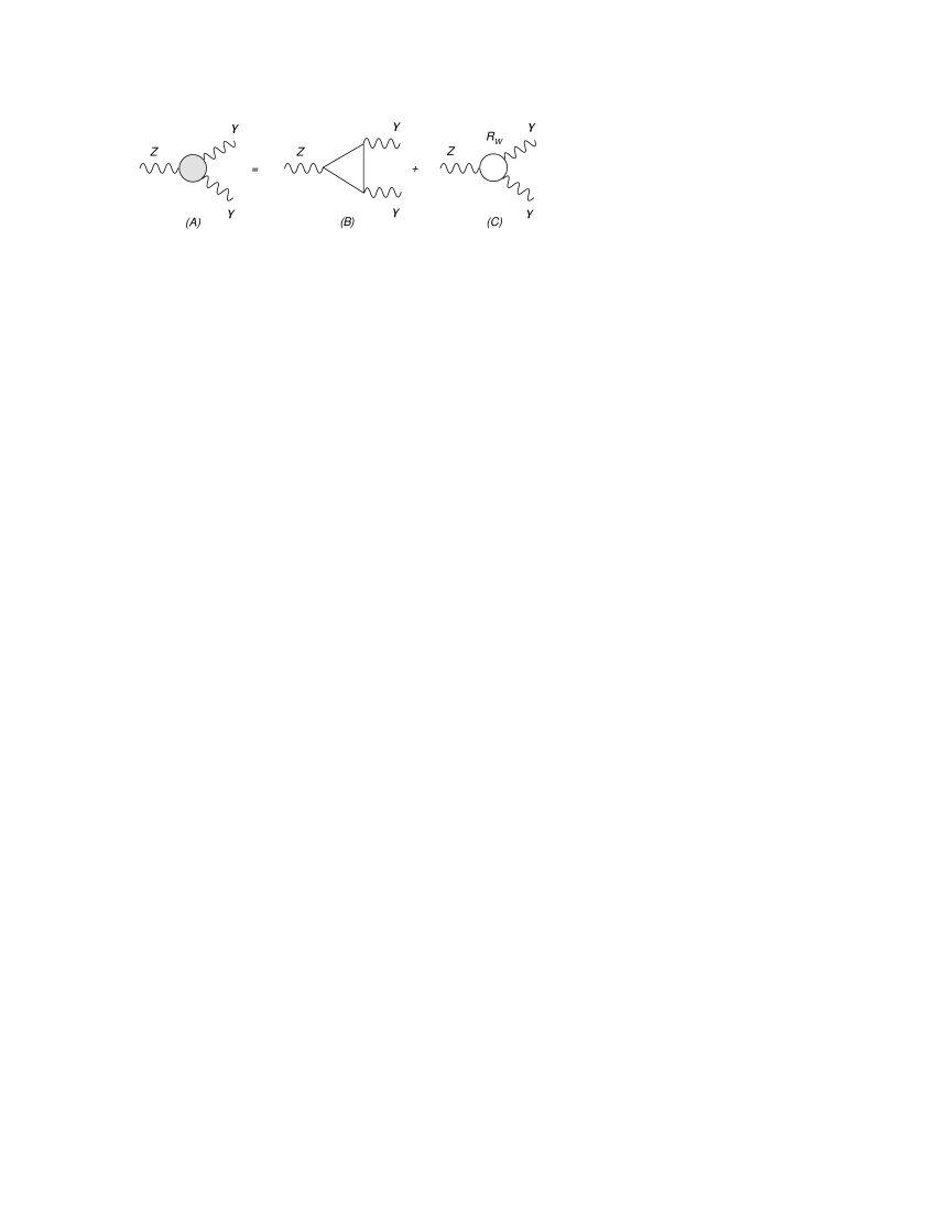
Figure 9: The $Z\gamma\gamma$ vertex to lowest order in the Standard Model, with the anomalous contributions and the remaining weak corrections shown separately.

Figure 10: Some typical electroweak corrections, involving the charged Goldstones (here denoted by $G$, ghosts contributions ($u_{\pm}$) and W exchanges.

Figure 11: $Z-G^{0}_{Z}$ mixing in the broken phase in the SM.

Figure 12: Same as in Fig. 11 but for the MLSOM

Figure 13: Re-distribution of the anomaly via the CS counterterm

$$G^{\rho\nu\mu}(k,k_{1},k_{2}) = -\frac{e^{2}g}{\cos\theta_{W}}\sum_{f}g^{f}_{A}Q^{2}_{f}\int\frac{d^{4}p}{(2\pi)^{4}}\,Tr\left(\frac{1}{{p\kern-4.30554pt\hbox{/}}-m_{f}}\gamma^{\rho}\gamma^{5}\frac{1}{{p\kern-4.30554pt\hbox{/}}-{k\kern-4.30554pt\hbox{/}}-m_{f}}\gamma^{\nu}\frac{1}{{p\kern-4.30554pt\hbox{/}}-{k\kern-4.30554pt\hbox{/}_{1}}-m_{f}}\gamma^{\mu}\right)$$ (110)

$$+\,(k_{1}\rightarrow k_{2},\mu\rightarrow\nu).$$

which can be cast in the form

$$G^{\rho\nu\mu}(k,k_{1},k_{2}) = -\frac{e^{2}g}{2\pi^{2}\cos{\theta_{W}}}\sum_{f}g^{f}_{A}Q^{2}_{f}\int^{1}_{0}dx_{1}\int^{1-x_{1}}_{0}dx_{2}\,$$ (111)

$$\cdot\,\frac{1}{\Delta}\,\Big{[}\epsilon^{\rho\nu\mu\alpha}(1-x_{1}-x_{2})(x_{2}k_{1}-x_{1}k_{2})_{\beta}(k^{\beta}_{2}k_{1\alpha}+k^{\beta}_{1}k_{2\alpha})$$

$$+(1-x_{1}-x_{2})(\epsilon^{\alpha\rho\beta\nu}k_{1\alpha}k_{2\beta}(x_{2}k^{\mu}_{1}-x_{1}k^{\mu}_{2})+(\mu\rightarrow\nu))$$

$$+\epsilon^{\alpha\nu\beta\mu}k_{1\alpha}k_{2\beta}(x_{2}(x_{2}-x_{1}-1)k^{\rho}_{1}-x_{1}(x_{2}-x_{1}+1)k^{\rho}_{2})\Big{]},$$

where

$$\Delta=m^{2}_{f}+x_{2}(x_{2}-1)k^{2}_{1}+x_{1}(x_{1}-1)k^{2}_{2}-2x_{1}x_{2}\,k_{1}\cdot k_{2},$$ (112)

and we have introducing the $g_{Z,A}^{f}$ and $g_{Z,V}^{f}$ couplings of the Z with

$$g_{Z,A}^{f}=\frac{1}{2}T_{3}^{f},\qquad g_{Z,V}^{f}=\frac{1}{2}T_{3}^{f}-Q_{f}\sin^{2}\theta_{W}.$$ (113)

This form of the amplitude is obtained if we use the standard Rosenberg definition of the anomalous diagrams and it agrees with [29]. In this case the Ward identities on the photon lines are defining conditions for the vertex. Naturally, with the standard fermion multiplet assignment the anomaly vanishes since

$$\sum_{f}g^{f}_{A}Q^{2}_{f}=0.$$ (114)

Because of the anomaly cancelation, the fermionic vertex is zero also off-shell, if the masses of all the fermions in each generation are degenerate, in particular if they are massless. Notice that this is not a consequence of the Landau-Yang theorem.

Let us now move to the Ward identity on the Z line. A direct computation gives

$$k_{\rho}\,G^{\rho\nu\mu} = (k_{1}+k_{2})_{\rho}\,G^{\,\rho\nu\mu}$$ (115)

$$= \frac{e^{2}g}{\pi^{2}\cos\theta_{W}}\sum_{f}g^{f}_{A}Q^{2}_{f}\,\epsilon^{\,\nu\mu\alpha\beta}k_{1\alpha}k_{2\beta}\,\left[\frac{1}{2}-m^{2}_{f}\int^{1}_{0}dx_{1}\int^{1-x_{1}}_{0}dx_{2}\,\frac{1}{\Delta}\right].$$

The presence of a mass-dependent term on the right hand side of (115) constitutes a break-down of axial current conservation for massive fermions, as expected.

7.1 The $Z\gamma\gamma$ vertex in anomalous abelian models: the Higgs-Stückelberg phase

The presence of anomalous generators in a given vertex renders some trilinear interactions non-vanishing also for massless fermions. In fact, as we have shown in the previous section, in the SM the anomalous triangle diagrams vanish if we neglect the masses of all the fermions, and this occurs both on-shell and off-shell. The only left over corrections are related to the fermion mass and these will also vanish (off-shell) if all the fermions of a given generation are mass degenerate. The on-shell vanishing of the same vertices is a consequence of the structure of the amplitude, as we show in the appendix. The extraction of the contribution of the anomalous generators in the trilinear vertices can be obtained starting from the 1-particle irreducible effective action, written in the basis of the interaction eigenstates, and performing the rotation of the trilinear interaction that project onto the $Z\gamma\gamma$ vertex.

In order to appreciate the differences between the SM result and the analogous one in the anomalous extensions that we are considering, we start by observing that only in the Stückelberg phase ($M_{1}\neq 0$ and $v_{u}=v_{d}=0$) the anomaly-free traces vanish,

$$\langle YYY\rangle\,g_{Y}^{3}\,Tr[Q_{Y}^{3}] = 0$$

$$\langle YW_{3}W_{3}\rangle\,g_{Y}g_{2}^{2}\,Tr[Q_{Y}T^{3}T^{3}] = 0\,,$$ (116)

because of charge assignment. A similar result is valid also in the HS phase if the Yukawa couplings are neglected. Coming to extract the $Z\gamma\gamma$ vertex we rotate the anomalous diagrams of the effective action into the mass eigenstates, being careful to separate the massless from the massive fermion contributions.

Hence, we split the $\langle YYY\rangle$ vertex into its chiral contributions and performing the rotation of the fields we get the following contributions

$$\frac{1}{3!}\,\langle YYY\rangle\,g_{Y}^{3}\,Tr[Q_{Y}^{3}]=$$

$$\hskip 71.13188pt\sum_{f}\left[g_{Y}^{3}\frac{1}{8}(Q_{Y,f}^{L})^{3}\langle LLL\rangle^{\lambda\mu\nu}+g_{Y}^{3}\frac{1}{8}(Q_{Y,f}^{R})^{3}\langle RRR\rangle^{\lambda\mu\nu}\right.$$

$$\hskip 71.13188pt\left.+g_{Y}^{3}\frac{1}{8}Q_{Y,f}^{L}(Q_{Y,f}^{R})^{2}\langle LRR\rangle^{\lambda\mu\nu}+g_{Y}^{3}\frac{1}{8}Q_{Y,f}^{L}Q_{Y,f}^{R}Q_{Y,f}^{L}\langle LRL\rangle^{\lambda\mu\nu}\right.$$

$$\hskip 71.13188pt\left.+g_{Y}^{3}\frac{1}{8}(Q_{Y,f}^{L})^{2}Q_{Y,f}^{R}\langle LLR\rangle^{\lambda\mu\nu}+g_{Y}^{3}\frac{1}{8}Q_{Y,f}^{R}(Q_{Y,f}^{L})^{2}\langle RLL\rangle^{\lambda\mu\nu}\right.$$

$$\hskip 71.13188pt\left.+g_{Y}^{3}\frac{1}{8}Q_{Y,f}^{R}Q_{Y,f}^{L}Q_{Y,f}^{R}\langle RLR\rangle^{\lambda\mu\nu}+g_{Y}^{3}\frac{1}{8}(Q_{Y,f}^{R})^{2}Q_{Y,f}^{L}\langle RRL\rangle^{\lambda\mu\nu}\right]Z^{\lambda}A_{\gamma}^{\mu}A_{\gamma}^{\nu}\frac{1}{3!}R^{YYY}+\dots$$

where the dots indicate all the other projections of the type $ZZ\gamma,Z^{\prime}\gamma\gamma$ etc. Here $\langle LLL\rangle$, $\langle RLR\rangle$ etc., indicate the (clockwise) insertion of $L/R$ chiral projectors on the $\lambda\mu\nu$ vertices of the anomaly diagrams.

For the $\langle YWW\rangle$ vertex the structure is more simple because the generator associated to $W_{3}$ is left-chiral

$$\frac{1}{2!}\,\langle YWW\rangle\,g_{Y}g_{2}^{2}\,Tr[Q_{Y}(T^{3})^{2}]=\sum_{f}\left[g_{Y}g_{2}^{2}\frac{1}{8}Q_{Y,f}^{L}(T^{3}_{L,f})^{2}\langle LLL\rangle^{\lambda\mu\nu}\right.$$

$$\left.\hskip 71.13188pt+g_{Y}g_{2}^{2}\frac{1}{8}Q_{Y,f}^{R}(T^{3}_{L,f})^{2}\langle RLL\rangle^{\lambda\mu\nu}\right]Z^{\lambda}A_{\gamma}^{\mu}A_{\gamma}^{\nu}\frac{1}{2!}R^{YWW}+\dots$$

The $\langle BYY\rangle$ vertex works in same way of $\langle YYY\rangle$

$$\frac{1}{2!}\,\langle BYY\rangle\,g_{B}g_{Y}^{2}\,Tr[Q_{B}Q_{Y}^{2}]=$$

$$\hskip 42.67912pt\sum_{f}\left[g_{B}g_{Y}^{2}\frac{1}{8}Q_{B,f}^{L}(Q_{Y,f}^{L})^{2}\langle LLL\rangle^{\lambda\mu\nu}+g_{B}g_{Y}^{2}\frac{1}{8}Q_{B,f}^{R}(Q_{Y,f}^{R})^{2}\langle RRR\rangle^{\lambda\mu\nu}\right.$$

$$\hskip 42.67912pt\left.+g_{B}g_{Y}^{2}\frac{1}{8}Q_{B,f}^{L}(Q_{Y,f}^{R})^{2}\langle LRR\rangle^{\lambda\mu\nu}+g_{B}g_{Y}^{2}\frac{1}{8}Q_{B,f}^{L}Q_{Y,f}^{R}Q_{Y,f}^{L}\langle LRL\rangle^{\lambda\mu\nu}\right.$$

$$\hskip 42.67912pt\left.+g_{B}g_{Y}^{2}\frac{1}{8}Q_{B,f}^{L}Q_{Y,f}^{L}Q_{Y,f}^{R}\langle LLR\rangle^{\lambda\mu\nu}+g_{B}g_{Y}^{2}\frac{1}{8}Q_{Y,f}^{R}(Q_{Y,f}^{L})^{2}\langle RLL\rangle^{\lambda\mu\nu}\right.$$

$$\hskip 42.67912pt\left.+g_{B}g_{Y}^{2}\frac{1}{8}Q_{B,f}^{R}Q_{Y,f}^{L}Q_{Y,f}^{R}\langle RLR\rangle^{\lambda\mu\nu}+g_{B}g_{Y}^{2}\frac{1}{8}Q_{B,f}^{R}Q_{Y,f}^{R}Q_{Y,f}^{L}\langle RRL\rangle^{\lambda\mu\nu}\right]Z^{\lambda}A_{\gamma}^{\mu}A_{\gamma}^{\nu}\frac{1}{2!}R^{BYY}+\dots$$

Finally, the $\langle BWW\rangle$ vertex is similar to $\langle YWW\rangle$

$$\frac{1}{2!}\,\langle BWW\rangle\,g_{Y}g_{2}^{2}\,Tr[Q_{B}(T^{3})^{2}]=\sum_{f}\left[g_{B}g_{2}^{2}\frac{1}{8}Q_{B,f}^{L}(T^{3}_{L,f})^{2}\langle LLL\rangle^{\lambda\mu\nu}\right.$$

$$\left.\hskip 142.26378pt+g_{B}g_{2}^{2}\frac{1}{8}Q_{B,f}^{R}(T^{3}_{L,f})^{2}\langle RLL\rangle^{\lambda\mu\nu}\right]Z^{\lambda}A_{\gamma}^{\mu}A_{\gamma}^{\nu}\frac{1}{2!}R^{BWW}+\dots$$

where we have defined

$$R^{YYY}=3\left[(O^{A\,T})_{22}(O^{A\,T})_{21}^{2}\right]$$

$$R^{YWW}=\left[2(O^{A\,T})_{11}(O^{A\,T})_{12}(O^{A\,T})_{21}+(O^{A\,T})_{11}^{2}(O^{A\,T})_{22}\right]$$

$$R^{BYY}=(O^{A\,T})_{21}^{2}(O^{A\,T})_{32}$$

$$R^{BWW}=\left[(O^{A\,T})_{11}^{2}(O^{A\,T})_{32}\right]\,.$$ (121)

which are the product of rotation matrices that project the anomalous effective action from the interaction eigenstate basis over the $Z,\gamma$ gauge bosons.

We have expressed the generators in their chiral basis, and their mixing is due to mass insertions over each fermion line in the loop. The ellypsis refers to additional contributions which do not project on the vertex that we are interested in but which are present in the analysis of the remaining neutral vertices, $ZZ\gamma,Z^{\prime}\gamma\gamma$ etc. The notation $O^{AT}$ indicates the transposed of the rotation matrix from the interaction to the mass eigenstates. To obtain the final expression of the amplitude in the interaction eigenstate basis one can easily observe that in the helicity conserving amplitudes $\langle LLL\rangle$ and $\langle RRR\rangle$ the mass dependence in the fermion loops is all contained in the denominators of the propagators, not in the Dirac traces. The only diagrams that contain a mass dependence at the numerators are those involving chirality flips ($\langle LLR\rangle,\langle RRL\rangle$) which contribute with terms proportional to $m_{f}^{2}$. These terms contribute only to the invariant amplitudes $A_{1}$ and $A_{2}$ of the Rosenberg representation [23] and, although finite, they disappear once we impose a Ward identity on the two photon lines, as requested by CVC for the two photons. A similar result is valid for the SM, as one can easily figure out from Eq. (111). Therefore, the amplitudes can be expressed just in terms of $LLL$ and $RRR$ correlators, and since the mass dependence is at the denominators of the propagators, one can easily show the relation

$$\langle LLL\rangle=-\langle RRR\rangle$$ (122)

valid for any fermion mass $m_{f}$. Defining $\langle LLL\rangle\equiv\Delta^{\lambda\mu\nu}_{LLL}(m_{f}\neq 0)$, we can express the only independent chiral graph as sum of two contributions

$$\Delta^{\lambda\mu\nu}_{LLL}(m_{f}\neq 0)=\Delta^{\lambda\mu\nu}_{LLL}(0)+\Delta^{\lambda\mu\nu}_{LLL}(m_{f})$$ (123)

where we define

$$\Delta^{\lambda\mu\nu}_{LLL}(0)\equiv\Delta^{\lambda\mu\nu}_{LLL}(m_{f}=0)$$

$$\Delta^{\lambda\mu\nu}_{LLL}(m_{f})\equiv\Delta^{\lambda\mu\nu}_{LLL}(m_{f}\neq 0)-\Delta^{\lambda\mu\nu}_{LLL}(m_{f}=0).$$ (124)

Also, one can verify quite easily that

$$\Delta^{\lambda\mu\nu}_{LLL}(0) = \Delta^{\lambda\mu\nu}_{AVV}(0)+\Delta^{\lambda\mu\nu}_{VAV}(0)+\Delta^{\lambda\mu\nu}_{VVA}(0)+\Delta^{\lambda\mu\nu}_{AAA}(0)$$

$$=4\Delta^{\lambda\mu\nu}_{AAA}(0).$$

A second contribution to the effective action comes from the 1-loop counterterms containing generalized CS terms. There are two ways to express these counterterms: either as separate 3-linear interactions or as modifications of the two invariant amplitudes of the Rosenberg parameterization $A_{1},A_{2}$. These amplitude depend linearly on the momenta of the vertex [23]. For instance we use

$$\Delta_{AAA}(0)-\frac{a_{n}}{3}\varepsilon^{\lambda\mu\nu\alpha}(k_{1\alpha}-k_{2\alpha})=\Delta_{AVV}(0),$$ (126)

which allows to absorb completely the CS term, giving conserved $Y/W_{3}$ currents in the interaction eigenstate basis. In this case we move from a symmetric distribution of the anomaly in the $AAA$ diagram, to an $AVV$ diagram. These currents interpolate with the vector-like vertices (V) of the AVV graph.

Notice that once the anomaly is moved from any vertex involving a $Y/W_{3}$ current to a vertex with a $B$ current, it is then canceled by the GS interaction. The extension of this analysis to the complete $m_{f}$-dependent case for $\Delta_{LLL}(m_{f}\neq 0)$ is quite straightforward. In fact, after some re-arrangements of the $Z\gamma\gamma$ amplitude, we are left with the following contributions in the physical basis in the broken phase

$$\langle Z\gamma\gamma\rangle|_{m_{f}\neq 0}=\frac{1}{4}\sum_{f}\Delta_{AVV}^{\lambda\mu\nu}(m_{f}\neq 0)\left[g_{Y}^{3}\theta_{f}^{YYY}R^{YYY}+g_{Y}g_{2}^{2}\theta_{f}^{YWW}R^{YWW}\right.$$

$$\hskip 56.9055pt\left.+g_{B}g_{Y}^{2}\theta_{f}^{BYY}R^{BYY}+g_{B}g_{2}^{2}\theta_{f}^{BWW}R^{BWW}\right]Z^{\lambda}A_{\gamma}^{\mu}A_{\gamma}^{\nu}$$ (127)

where we have defined the anomalous chiral asymmetries as

$$\theta^{BYY}_{f}=\left[Q_{B,f}^{L}(Q_{Y,f}^{L})^{2}-Q_{B,f}^{R}(Q_{Y,f}^{R})^{2}\right]$$

$$\theta^{BWW}_{f}=Q_{B,f}^{L}(T^{3}_{L,f})^{2}.$$ (128)

The conditions of gauge invariance force the coefficients in front of the CS terms to be

$$D_{BYY}=\frac{1}{8}\sum_{f}\theta^{BYY}_{f}$$

$$D_{BWW}=\frac{1}{8}\sum_{f}\theta^{BWW}_{f},\,$$ (129)

which have been absorbed and do not appear explicitly, while the SM chiral asymmetries are defined as

$$\theta^{YYY}_{f}=\left[(Q_{Y,f}^{L})^{3}-(Q_{Y,f}^{R})^{3}\right]$$

$$\theta^{YWW}_{f}=Q_{Y,f}^{L}(T^{3}_{L,f})^{2},$$ (130)

and the triangle $\Delta_{AVV}(m_{f}\neq 0)$ is given as in (111). Notice that Eq. (127) is in complete agreement with the SM result shown in (111), obtained by removing the contributions proportional to the $B$ gauge bosons and setting the chiral asymmetries of $Y$ and $W_{3}$ to zero. In particular, if the gauge bosons are not anomalous and in the chiral limit ($m_{f}=0$ or $m_{f}=m$) this trilinear amplitude vanishes.

As we have already pointed out, the amplitude for the $\langle Z\gamma\gamma\rangle$ process is espressed in terms of 6 invariant amplitudes that can be easily computed and take the form

$$\Delta^{\lambda\mu\nu}_{AVV} = {A}_{1}(k_{1},k_{2})\epsilon[k_{1},\mu,\nu,\lambda]+{A}_{2}(k_{1},k_{2})\epsilon[k_{2},\mu,\nu,\lambda]+{A}_{3}(k_{1},k_{2})\epsilon[k_{1},k_{2},\mu,\lambda]{k_{1}}^{\nu}$$

$$+{A}_{4}(k_{1},k_{2})\epsilon[k_{1},k_{2},\mu,\lambda]{k_{2}}^{\nu}+{A}_{5}(k_{1},k_{2})\epsilon[k_{1},k_{2},\nu,\lambda]k_{1}^{\mu}+{A}_{6}(k_{1},k_{2})\epsilon[k_{1},k_{2},\nu,\lambda]k_{2}^{\mu},$$

with

$$A_{1}(k_{1},k_{2}) = k_{1}\cdot k_{2}A_{3}(k_{1},k_{2})+k_{2}^{2}A_{4}(k_{1},k_{2})$$

$$A_{2}(k_{1},k_{2}) = -A_{1}(k_{2},k_{1})$$

$$A_{5}(k_{1},k_{2}) = -A_{4}(k_{2},k_{1})$$

$$A_{6}(k_{1},k_{2}) = -A_{3}(k_{2},k_{1}).$$

Also $A_{1}(k_{1},k_{2})=A_{1}(k_{2},k_{1})$ as one can easily check by a direct computation. We obtain

$$A_{3}(k_{1},k_{2})=-\frac{1}{2}\int_{0}^{1}dx\int_{0}^{1-x}dy\frac{xy}{y(1-y)k_{1}^{2}+x(1-x)k_{2}^{2}+2xy\,k_{1}\cdot k_{2}-m_{f}^{2}}$$

$$A_{4}(k_{1},k_{2})=\frac{1}{2}\int_{0}^{1}dx\int_{0}^{1-x}dy\frac{x(1-x)}{y(1-y)k_{1}^{2}+x(1-x)k_{2}^{2}+2xy\,k_{1}\cdot k_{2}-m_{f}^{2}}$$

The computation of these integrals can be done analytically and the various regions $0<s<4m_{f}^{2}$, $m_{f}>>\sqrt{s}/2$, and $m_{f}\to 0$ can be studied in detail. In the case of both photons on-shell, for instance, and $s>4m_{f}^{2}$ we obtain

$$A_{3}(k_{1},k_{2})=\frac{1}{2s}-\frac{m_{f}^{2}}{s}\makebox{Li}_{2}\left(\frac{2}{1-\sqrt{1-4m_{f}^{2}/s}}\right)-\frac{m_{f}^{2}}{s}\makebox{Li}_{2}\left(\frac{2}{1+\sqrt{1-4m_{f}^{2}/s}}\right)$$

$$A_{4}(k_{1},k_{2})=-\frac{1}{s}+\frac{\sqrt{1-4m_{f}^{2}/s}}{s}\makebox{ArcTanh}\left(\frac{1}{\sqrt{1-4m_{f}^{2}/s}}\right)$$ (134)

Notice that the case in which the two photons are on-shell and light fermions are running in the loop, then the evaluation of the integral requires particular care because of infrared effects which render the parameteric integrals ill-defined. The situation is similar to the case of the coupling of the axial anomaly to on-shell gluons in spin physics [30], when the correct isolation of the massless quarks contributions is carried out by moving off-shell on the external lines and then performing the $m_{f}\to 0$ limit.

7.2 $q\bar{q}\to\gamma\gamma$ with an intermediate Z

In this section we are going to describe the role played by the new anomaly cancelation mechanism in simple processes which can eventually be studied with accuracy at a hadron collider such as the LHC. A numerical analysis of processes involving neutral currents can be performed along the lines of [9] and we hope to return to this point in the near future. Here we intend to discuss briefly some of the phenomenological implications which might be of interest. Since the anomaly is canceled by a combination of Chern-Simons and Green-Schwarz contributions, the study of a specific process, such as $Z\to\gamma\gamma$, which differs from the SM prediction, requires, in general, a combined analysis both of the gauge sector and of the scalar sector.

We start from the case of a quark-antiquark annihilation mediated by a Z that later undergoes a decay into two photons. At leading order this process is at parton level described by the annihilations of a valence quark $q$ and a sea antiquark $\bar{q}$ from the two incoming hadrons, both of them collinear and massless. In Fig. (14) we have depicted all the diagrams by which the process can take place to lowest order. Radiative corrections from the initial state are accurately known up to next-to-next-to-leading order, and are universal, being the same of the Drell-Yan cross section. In this respect, precise QCD predictions for the rates are available, for instance around the Z resonance [9].

In the SM, gauge invariance of the process requires both a $Z$ gauge boson exchange and the exchange of the corresponding goldstone $G_{Z}$, which involves diagrams (A) and (B). In the MLSOM a direct Green-Schwarz coupling to the photon (which is gauge dependent) is accompanied by a gauge independent axion exchange. If the incoming quark-antiquark pair is massless, then the Goldstone has no coupling to the incoming fermion pair, and therefore (B) is absent, while gauge invariance is trivially satisfied because of the massless condition on the fermion pair of the initial state. In this case only diagram (A) is relevant. Diagram (B) may also be set to vanish, for instance in suitable gauges, such as the unitary gauge. Notice also that the triangle diagrams have a dependence on $m_{f}$, the mass of the fermion in the loop, and show two contributions: a first contribution which is proportional to the anomaly (mass independent) and a correction term which depends on $m_{f}$.

As we have shown above, the first contribution, which involves an off-shell vertex, is absent in the SM, while it is non vanishing in the MLSOM. In both cases, on the other hand, we have $m_{f}$ dependent contributions. It is then clear that in the SM the largest contribution to the process comes from the top quark circulating in the triangle diagram, the amplitude being essentially proportional only to the heavy top mass. On the $Z$ resonance and for on-shell photons, the cross section vanishes in both cases, as we have explained, in agreement with the Landau-Yang theorem. We have checked these properties explicitly, but they hold independently of the perturbative order at which they are analyzed, being based on the Bose symmetry of the two photons. The cross section, therefore, has a dip at $Q=M_{Z}$, where it vanishes, and where $Q^{2}$ is the virtuality of the intermediate s-channel exchange.

An alternative scenario is to search for neutral exchanges initiated by gluon-gluon fusion. In this case we replace the annihilation pair with a triangle loop (the process is similar to Higgs production via gluon fusion), as shown in Fig. 15. As in the decay mechanism discussed above, the production mechanism in the SM and in the MLSOM are again different. In fact, in the MLSOM there is a massless contribution appearing already at the massless fermion level, which is absent in the SM. The production mechanism by gluon fusion has some special features as well. In ggZ production and $Z\gamma\gamma$ decay, the relevant diagrams are (A) and (B) since we need the exchange of a $G_{Z}$ to obtain gauge invariance. As we probe smaller values of the Bjorken variable $x$, the gluon density raises, and the process becomes sizable. On the other hand, in a pp collider, although the quark annihilation channel is suppressed since the antiquark density is smaller than in a $p\bar{p}$ collision, this channel still remains rather significant. We have also shown in this figure one of the scalar channels, due to the exchange of a axi-Higgs.

Other channels such as those shown in Fig. 16 can also be studied, these involve a lepton pair in the final state, and their radiative corrections also show the appearance of a triangle vertex. This is the classical Drell-Yan process, that we will briefly describe below. In this case, both the total cross section and the rapidity distributions of the lepton pair and/or an analysis of the charge asymmetry in s-channel exchanges of W’s would be of major interest in order to disentangle the anomaly inflow. At the moment, errors on the parton distributions and scale dependences induce indeterminations which, just for the QCD background, are around $4\%$ [9], as shown in a high precision study. It is expected, however, that the statistical accuracy on the $Z$ resonance at the LHC is going to be a factor 100 better. In fact this is a case in which the experiment can do better than the theory.

7.3 Isolation of the massless limit: the $Z^{*}\to\gamma^{*}\gamma^{*}$ amplitude

The isolation of the massless from the massive contributions can be analized in the case of resolved photons in the final state. As we have already mentioned in the prompt photon case the amplitude, on the Z resonance, vanishes because of Bose symmetry and angular momentum conservation. We can, however, be on the $Z$ resonance and produce one or two off-shell photons that undergo fragmentation. Needless to say, these contributions are small. However, the separation of the massless from the massive case is well defined. One can increase the rates by asking just for 1 single resolved photon and 1 prompt photon. Rates for this process in pp-collisions have been determined in [31]. We start from the case of off-shell external photons of virtuality $s_{1}$ and $s_{2}$ and an off-shell Z $(Z^{*})$. Following [32], we introduce the total vertex $V^{\lambda\mu\nu}(k_{1},k_{2},m_{f})$, which contains both the massive $m_{f}$ dependence (corresponding to the triangle amplitude $\Delta^{\lambda\mu\nu}$. Its massless counterpart ${\bf V}^{\lambda\mu\nu}(0)\equiv V(k_{1},k_{2},m_{f}=0)$, obtained by sending the fermion mass to zero. The Rosenberg vertex and the V vertex are trivially related by a Schoutens transformation, moving the $\lambda$ index from the Levi-Civita tensor to the momenta of the photons

$$V_{\lambda\mu\nu}(k_{1},k_{2},m_{f})$$

$$=A(k_{1},k_{2},m_{f})\varepsilon[\lambda,\mu,\nu,k_{2}]s_{1}-A(k_{2},k_{1},m_{f})\varepsilon[\lambda,\mu,\nu,k_{1}]s_{2}+A(k_{1},k_{2},m_{f})\varepsilon[\lambda,\nu,k_{1},k_{2}]k_{1}^{\mu}$$

$$+A(k_{2},k_{1},m_{f})\varepsilon[\lambda,\mu,k_{2},k_{1}]k^{\nu}_{2}-B(k_{1},k_{2},m_{f})\varepsilon[\mu,\nu,k_{1},k_{2}]k^{\lambda}$$ (135)

with $k-k_{1}-k_{2}=0$ and $s_{i}=k_{i}^{2}\,\,(i=1,2)$, and

$$A(k_{1},k_{2},m_{f}) = \frac{1}{\lambda}\left[-\frac{1}{2}(s-s_{1}+s_{2})-\left(\frac{1}{2}(s+s_{2})+(6/{\lambda})ss_{1}s_{2}\right)\Delta_{\#1}\right.$$ (136)

$$+s_{2}\left[\frac{1}{2}-(3/{\lambda})s(s-s_{1}-s_{2})\right]\Delta_{\#2}$$

$$\left.+\left[ss_{2}+(m_{f}^{2}+(3/{\lambda})ss_{1}s_{2})(s-s_{1}+s_{2})\right]C_{\#0}\right]$$

$$B(k_{1},k_{2},m_{f}) = \frac{1}{\lambda}\left[\frac{1}{2}(s-s_{1}-s_{2})+s_{1}\left[\frac{1}{2}+(3/{\lambda})s_{2}(s+s_{1}-s_{2})\right]\Delta_{\#1}\right.$$ (137)

$$+s_{2}\left[\frac{1}{2}+(3/{\lambda})s_{1}(s-s_{1}+s_{2})\right]\Delta_{\#2}$$

$$\left.+\left[s_{1}s_{2}-(m_{f}^{2}+(3/{\lambda})ss_{1}s_{2})(s-s_{1}-s_{2})\right]C_{\#0}\right]$$

with

$$\lambda=\lambda(s,s_{1},s_{2}),\\$$

being the usual Mandelstam function and where the analytic expressions for $\Delta_{\#i}$ and $C_{\#0}$ are given by

$$\Delta_{\#i} = a_{i}\,\mbox{ln}\frac{a_{i}+1}{a_{i}-1}-a_{3}\,\mbox{ln}\frac{a_{3}+1}{a_{3}-1},\,\,\,\mbox{(i=1,2)}$$

$$C_{\#0} = \frac{1}{\sqrt{\lambda}}\sum^{3}_{i=1}\left[\mbox{ Li}_{2}\left(\frac{b_{i}-1}{a_{i}+b_{i}}\right)-\mbox{Li}_{2}\left(\frac{-b_{i}-1}{a_{i}-b_{i}}\right)+\mbox{Li}_{2}\left(\frac{-b_{i}+1}{a_{i}-b_{i}}\right)-\mbox{Li}_{2}\left(\frac{b_{i}+1}{a_{i}+b_{i}}\right)\right],$$

and

$$t_{i}=-s_{i}-i\epsilon,\qquad a_{i}=\sqrt{1+(2m_{f})^{2}/t_{i}},\,\,\mbox{(i=1,2,3)},$$

$$\lambda=\lambda(t_{1},t_{2},t_{3}),\qquad b_{1}=(t_{1}-t_{2}-t_{3})/\sqrt{\lambda}\,\,\,\,\mbox{or cyclic}$$ (139)

For $m_{f}=0$ the two expressions above become

$$\Delta_{\#i} = \mbox{ln}(t_{i}/t_{3}),\,\,\,(i=1,2),$$

$$C_{\#0} = (1/\sqrt{\lambda})\Biggr{[}2\Biggr{(}\zeta(2)-\mbox{Li}_{2}(x_{1})-\mbox{Li}_{2}(x_{2})+\mbox{Li}_{2}\left(\frac{1}{x_{3}}\right)\Biggr{)}+\mbox{ln}x_{1}\mbox{ln}x_{2}\Biggr{]}$$ (140)

with

$$x_{i}=\frac{(b_{i}+1)}{(b_{i}-1)},\,\,\,(i=1,2,3).$$ (141)

These can be inserted into (136) and (137) together with $m_{f}=0$ to generate the corresponding ${\bf V}^{\lambda\mu\nu}(0)$ vertex needed for the computation of the massless contributions to the amplitude.

With these notations we clearly have

$$\Delta^{\lambda\mu\nu} = V^{\lambda\mu\nu}(k_{1},k_{2},m_{f})$$

$$\Delta^{\lambda\mu\nu}(0) = {\bf V}^{\lambda\mu\nu}(k_{1},k_{2})$$

$$\Delta^{\lambda\mu\nu}(m_{f}) = V^{\lambda\mu\nu}(k_{1},k_{2},m_{f})-{\bf V}^{\lambda\mu\nu}(k_{1},k_{2}).$$

7.4 Extension to $Z\to\gamma^{*}\gamma$

To isolate the contribution to the decay on the resonance, we keep one of the two photons off-shell (resolved). We choose $s_{1}=0$, and $s_{2}$ virtual. We denote by $\Gamma^{\lambda\mu\nu}$ the corresponding vertex in this special kinematical configuration. The Z boson is on-shell. In this case at 1-loop the result simplifies considerably [33]

$$\Gamma_{\lambda\mu\nu} = F_{2}(s_{2}\epsilon[\lambda,\mu,\nu,k_{1}]+k^{\nu}_{2}\epsilon[\lambda,\mu,k_{1},k_{2}]),$$ (143)

with $F_{2}$ expressed as a Feynman parametric integral

$$F_{2}=\frac{1}{{2\pi^{2}}}\int^{1}_{0}dz_{1}dz_{2}dz_{3}\delta(1-z_{1}-z_{2}-z_{3})\frac{-z_{2}z_{3}}{m_{f}^{2}-z_{2}z_{3}s_{2}-z_{1}z_{3}M_{Z}^{2}}.$$ (144)

Setting $F_{2}\equiv-F(z,r_{f})$ where $f(z,r)$ is a dimensionless function of

$$z=s_{2}/M^{2}_{Z},\qquad r_{f}=m^{2}_{Z}/4m_{f}^{2},$$ (145)

and for vanishing $m_{f}$ ($r_{f}=M^{2}_{Z}/4m^{2}_{f}\rightarrow\infty$), the corresponding massless contribution is expressed as $F(z,\infty)$ with, in general

$$F(z,r_{f})=\frac{1}{4(1-z)^{2}}(I(r_{f}z,r_{f})-I(r_{f},r_{f})+1-z),$$ (146)

where

$$I(x,r_{f}) = 2\sqrt{\frac{x-1}{x^{-}}}\mbox{ln}(\sqrt{-x}+\sqrt{1-x})-\frac{1}{r_{f}}(\mbox{ln}(\sqrt{-x}+\sqrt{1-x}))^{2}\,\,\,\,\,\,\,\,\mbox{for \,x $<$ 0}$$ (147)

$$= 2\sqrt{\frac{1-x}{x}}\sin^{-1}\sqrt{x}+\frac{1}{r_{f}}(\sin^{-1}\sqrt{x})^{2}\,\,\,\,\,\,\,\mbox{for 0$<$\,x $<$ 1}$$

$$= 2\sqrt{\frac{x-1}{x}}\left(\ln(\sqrt{x}+\sqrt{x-1})-\frac{i\pi}{2}\right)-\frac{1}{r_{f}}\left(\ln(\sqrt{x}+\sqrt{x-1})-\frac{i\pi}{2}\right)^{2},$$

$$\,\,\mbox{for \,x $>$ 1}.$$

The $m_{f}=0$ contribution is obtained in the $r_{f}\rightarrow+\infty$ limit,

$$F(z,\infty) = \frac{1}{4(1-z)^{2}}(\ln z+1-z)\,\,\,\,\,\,\,\,\,\,\,\,\,\,\,\,\,\,\mbox{for \, z $>$ 0},$$ (148)

$$= \frac{1}{4(1-z)^{2}}(\ln|z|+i\pi+1-z)\,\,\,\,\,\,\,\mbox{for \, z $<$ 0}.$$

In these notations, the infinite fermion mass limit ($m_{f}\rightarrow\infty$ or $r\rightarrow 0$), gives $F(z,0)=0$ and we find

$$\Delta^{\lambda\mu\nu} = \Gamma^{\lambda\mu\nu}=F(z,r_{f})$$

$$\Delta^{\lambda\mu\nu}(0) = {\Gamma}^{\lambda\mu\nu}(0)=F(z,\infty)$$

$$\Delta^{\lambda\mu\nu}(m_{f}) = \Gamma^{\lambda\mu\nu}-\Gamma^{\lambda\mu\nu}(m_{f})=F(z,r_{f})-F(z,\infty),$$ (149)

which can be used for a numerical evaluation. The decay rate for the process is given by

$$\Gamma(Z\to\gamma^{*}\gamma)=\frac{1}{4M_{Z}}\int d^{4}k_{1}d^{4}k_{2}\delta(k_{1}^{2})\,\delta(k_{2}^{2}-Q_{*}^{2})|{\cal M}_{Z\to\gamma\gamma^{*}}|^{2}\,2(\pi)^{4}\delta(k-k_{1}-k_{2}),$$ (150)

where

$$|{\cal M}_{Z\to\gamma\gamma^{*}}|^{2} = -A^{\lambda\mu\nu}_{Z\to\gamma\gamma^{*}}\Pi_{Z}^{\lambda\lambda^{\prime}}A^{\lambda^{\prime}\mu\nu^{\prime}}_{Z\to\gamma\gamma^{*}}\Pi_{Q^{*}}^{\nu\nu^{\prime}}$$

$$\Pi_{Z}^{\lambda\lambda^{\prime}} = -g^{\lambda\lambda^{\prime}}+\frac{k^{\lambda}k^{\lambda^{\prime}}}{M_{Z}^{2}}$$

$$\Pi_{Q^{*}}^{\nu\nu^{\prime}} = -g^{\lambda\lambda^{\prime}}+\frac{k^{\lambda}k^{\lambda^{\prime}}}{Q_{*}^{2}}.$$ (151)

We have indicated with $Q_{*}$ the virtuality of the photon. A complete evaluation of this expression, to be of practical interest, would need the fragmentation functions of the photon (see [31] for an example). A detailed analysis of these rates will be presented elsewhere. However, we will briefly summarize the main points involved in the analysis of this and similar processes at the LHC, where the decay rate is folded with the (NLO/NNLO) contribution from the initial state using QCD factorization.

Probably one of the best way to search for neutral current interactions in hadronic collisions at the LHC is in lepton pair production via the Drell-Yan mechanism. QCD corrections are known for this process up to O($\alpha_{s}^{2}$) (next-to-next-to-leading order, NNLO), which can be folded with the NNLO evolution of the parton distributions to provide accurate determinations of the hadronic pp cross sections at the 4 $\%$ level of accuracy [9]. The same computation for Drell-Yan can be used to analize the $pp\to Z\to\gamma\gamma^{*}$ process since the $W_{V}$ (hadronic) part of the process is universal, with $W_{V}$ defined below. An appropriate (and very useful) way to analyze this process would be to perform this study defining the invariant mass distribution

$$\frac{d\sigma}{dQ^{2}}=\tau\sigma_{Z\to\gamma^{*}\gamma}(Q^{2},M_{V}^{2})\,W_{V}(\tau,Q^{2})$$ (152)

where $\tau=Q^{2}/S$, which is separated into a pointlike contribution $\sigma_{Z\to\gamma\gamma^{*}}$

$$\sigma_{V}(Q^{2},M_{V}^{2})=\frac{\pi\alpha}{4M_{Z}\sin\theta_{W}^{2}\cos\theta_{W}^{2}N_{c}}\frac{\Gamma(Z\to\gamma\gamma^{*})}{(Q^{2}-M_{Z}^{2})^{2}+M_{Z}^{2}\Gamma_{Z}^{2}}.$$ (153)

and a hadronic structure functions $W_{Z}$. This is defined via the integral over parton distributions and coefficient functions $\Delta_{ij}$

$$W_{Z}(Q^{2},M_{Z}^{2})=\int_{0}^{1}dx_{1}\,\int_{0}^{1}dx_{2}\int_{0}^{1}dx\delta(\tau-xx_{1}x_{2})PD^{V}_{ij}(x_{1},x_{2},\mu_{f}^{2})\Delta_{ij}(x,Q^{2},\mu_{f}^{2})$$ (154)

where $\mu_{f}$ is the factorization scale. The choice $\mu_{f}=Q$, with Q the invariant mass of the $\gamma\gamma^{*}$ pair , removes the $\log(Q/M)$ for the computation of the coefficient functions, which is, anyhow, arbitrary. The non-singlet coefficient functions are given by

$$\Delta^{(0)}_{q\bar{q}} = \delta(1-x)$$

$$\Delta^{(1)}_{q\bar{q}} = \frac{\alpha_{S}(M_{V}^{2})}{4\pi}C_{F}\left[\delta(1-x)(8\zeta(2)-16)+16\left(\frac{\log(1-x)}{1-x}\right)_{+}\right.$$ (155)

$$\left.\qquad\qquad\quad\qquad-8(1+x)\log(1-x)-4\frac{1+x^{2}}{1-x}\log x\right]$$

with $C_{F}=(N_{c}^{2}-1)/(2N_{c})$ and the “+” distribution is defined by

$$\left(\frac{\log(1-x)}{1-x}\right)_{+}=\theta(1-x)\frac{\log(1-x)}{1-x}-\delta(1-x)\int_{0}^{1-\delta}dx\,\frac{\log(1-x)}{1-x},$$ (156)

while at NLO appears also a q-g sector

$$\Delta^{(1)}_{qg}=\frac{\alpha_{S}(M_{V}^{2})}{4\pi}T_{F}\left[2(1+2x^{2}-2x)\log\left(\frac{(1-x)^{2}}{x}\right)+1-7x^{2}+6x\right].$$ (157)

Other sectors do not appear at this order. Explicitly one gets

$$W_{Z}(Q^{2},M_{Z}^{2}) = \sum_{i}\int_{0}^{1}dx_{1}\,\int_{0}^{1}dx_{2}\int_{0}^{1}dx\delta(\tau-xx_{1}x_{2})$$

$$\times\Big{\{}\bigg{(}q_{i}(x_{1},\mu_{f}^{2})\bar{q_{i}}(x_{2},\mu_{f}^{2})+\bar{q_{i}}(x_{1},\mu_{f}^{2}){q_{i}}(x_{2},\mu_{f}^{2})\bigg{)}\Delta_{q\bar{q}}(x,Q^{2},\mu_{f}^{2})$$

$$\qquad+\bigg{(}q_{i}(x_{1},\mu_{f}^{2}){g}(x_{2},\mu_{f}^{2})+{q_{i}}(x_{2},\mu_{f}^{2}){g}(x_{1},\mu_{f}^{2})\bigg{)}\Delta_{q{g}}(x,Q^{2},\mu_{f}^{2})\Big{\}}$$

where the sum is over the quark flavours. The identification of the generalized mechanism of anomaly cancelation requires that this description be extended to NNLO, which is now a realistic possibility. It involves a slight modification of the NNLO hard scatterings known at this time and an explicit computation is in progress.

Figure 14: Two photon processes initiated by a $q\bar{q}$ annihilation with a $Z$ exchange.

Figure 15: Gluon fusion contribution to double-photon production. Shown are also the scalar exchanges (B) and (D) that restore gauge invariance and the axi-Higgs exchange (E).

Figure 16: The $q\bar{q}$ annihilation channel (A,B). Scalar exchanges in the neutral sector involving the two Higsses and the Axi-Higgs (C,D,E).

8 Conclusions

We have presented a study of a model inspired by the structure encountered in a typical string theory derivation of the Standard Model. In particular we have focused our investigation on the characterization of the effective action and worked out its expression in the context of an extension containing one additional anomalous $U(1)$. Our analysis specializes and, at the same time, extends a previous study of models belonging to this class. The results that we have presented are generic for models where the Stückelberg and the Higgs mechanism are combined and where an effective abelian anomalous interaction is present. Our analysis has then turned toward the study of simple processes mediated by neutral current exchanges, and we have focused, specifically, on one of them, the one involving the $Z\gamma\gamma$ vertex. In particular our findings clearly show that new massless contributions are presented at 1-loop level when anomalous generators are involved in the fermionic triangle diagrams and the interplay between massless and massive fermion effects is modified respect to the SM case. The typical processes considered in our analysis deserve a special attention, given the forthcoming experiments at the LHC, since they may provide a way to determine whether anomaly effects are present in some specific reactions. Other similar processes, involving the entire neutral sector should be considered, though the two-photon signal is probably the most interesting one phenomenologically.

Given the high statistical precision ($.05\%$ and below on the Z peak, for 10 $fb^{-1}$ of integrated luminosity) which can be easily obtained at the LHC, there are realistic chances to prove or disprove theories of these types. Concerning the possibility of discovering extra anomalous $Z^{\prime}$, although there are stringent upper bounds on their mixing(s) with the Z gauge boson, it is of outmost importance to bring this type of analysis even closer to the experimental test by studying in more detail the peculiarities of anomalous gauge interactions for both the neutral and the charged sectors along the lines developed in this work. This analysis is in progress and we hope to report on it in the near future.

Acknowledgements

We dedicate this work to the memory of Hidenaga Yamagishi, remembering his remarkable scientific talent, his outstanding human qualities and his unique and inspirational love for physics.

We thank Elias Kiritsis for having brought the topics discussed in this work to our attention and Theodore Tomaras, Marco Roncadelli, Marco Guzzi, Roberta Armillis, Andrea Spirito and Antonio Quintavalle for discussions. The work of C.C. was supported in part by the European Union through the Marie Curie Research and Training Network “Universenet” (MRTN-CT-2006-035863). He thanks the Theory Group at the University of Liverpool and in particular Alon Faraggi for discussions and for the kind hospitality. N.I. was partially supported by the European contract MRTN-CT-2004-512194.

9 Appendix. A Summary on the single anomalous $U(1)$ model.

We summarize in this appendix some results concerning the model with a single anomalous $U(1)$ discussed in the main sections. These results specialize and simplify the general discussion of [19] to which we refer for further details. We will use the hypercharge values

$f$	$Q_{L}$	$u_{R}$	$d_{R}$	$L$	$e_{R}$	$\nu_{R}$
$q_{Y}$	$1/6$	$2/3$	$-1/3$	$-1/2$	$-1$	$0$

and general $U(1)_{B}$ charge assignments

$f$	$Q_{L}$	$u_{R}$	$d_{R}$	$L$	$e_{R}$	$\nu_{R}$
$q_{B}$	$q^{(Q_{L})}_{B}$	$q^{(u_{R})}_{B}$	$q^{(d_{R})}_{B}$	$q^{(L)}_{B}$	$q^{(e_{R})}_{B}$	$q^{(\nu_{R})}_{B}$

The covariant derivatives act on the fermions $f_{L},f_{R}$ as

$${\cal D}_{\mu}f_{L}=\left(\partial_{\mu}+i{\bf A}_{\mu}+iq_{l}^{(f_{L})}g_{l}A_{l,\mu}\right)f_{L}$$

$${\cal D}_{\mu}f_{R}=\left(\partial_{\mu}+i{\bf A}_{\mu}+iq_{l}^{(f_{R})}g_{l}A_{l,\mu}\right)f_{R}$$ (159)

with $l=Y,B$ abelian index, where ${\bf A}_{\mu}$ is a non-abelian Lie algebra element and write the lepton doublet as

$$L_{i}=\pmatrix{\nu_{Li}\cr e_{Li}}.$$ (160)

We will also use standard notations for the $SU(2)_{W}$ and $SU(3)_{C}$ gauge bosons

$$W_{\mu} = \frac{\sigma_{i}}{2}W^{i}_{\mu}=\tau_{i}W^{i}_{\mu},\;\;\;\;\;\mbox{with}\;\;\;\;i=1,2,3$$ (161)

$$G_{\mu} = \frac{\lambda_{a}}{2}G^{\,a}_{\mu}=T_{a}G^{\,a}_{\mu}\;\;\;\;\;\mbox{with}\;\;\;\;a=1,2,...,8$$ (162)

with the normalizations

$$Tr[\tau^{i}\tau^{j}]=\frac{1}{2}\delta_{ij},\qquad Tr[T^{a}T^{b}]=\frac{1}{2}\delta_{ab}.$$ (163)

The interaction lagrangean for the leptons becomes

$${\cal L}_{int}^{lep} = \pmatrix{\overline{{\nu}}_{Li}&\overline{e}_{Li}}\gamma^{\mu}\left[-g_{2}\frac{\tau^{a}}{2}W_{\mu}^{a}-g_{Y}\,q^{(L)}_{Y}A^{Y}_{\mu}-g_{B}q^{(L)}_{B}B_{\mu}\right]\pmatrix{\nu_{Li}\cr e_{Li}}+$$ (164)

$$+\;\overline{e}_{Ri}\;\gamma^{\mu}\left[-g_{Y}q^{(e_{R})}_{Y}A^{Y}_{\mu}-g_{B}q^{(e_{R})}_{B}B_{\mu}\right]e_{Ri}$$

$$+\;\overline{\nu}_{Ri}\;{\gamma}^{\mu}\left[-g_{Y}q^{({\nu}_{R})}_{Y}A^{Y}_{\mu}-g_{B}q^{(\nu_{R})}_{B}B_{\mu}\right]{\nu}_{Ri}.$$

As usual we define the left-handed and right-handed currents

$$J^{L}_{\mu}=\frac{1}{2}(J_{\mu}-J^{5}_{\mu}),\qquad J^{R}_{\mu}=\frac{1}{2}(J_{\mu}+J^{5}_{\mu}),\qquad J_{\mu}=J^{R}_{\mu}+J^{L}_{\mu},\qquad J^{5}_{\mu}=J^{R}_{\mu}-J^{L}_{\mu}.$$ (165)

Writing the quark doublet as

$$Q_{Li}=\pmatrix{u_{Li}\cr d_{Li}},$$ (166)

we obtain the interaction lagrangean

$${\cal L}_{int}^{quarks} = \pmatrix{\overline{u}_{Li}&\overline{d}_{Li}}\gamma^{\mu}\left[-g_{3}\frac{\lambda^{a}}{2}G^{a}_{\mu}-g_{2}\frac{\tau^{i}}{2}W_{\mu}^{i}-g_{Y}\,q^{(Q_{L})}_{Y}A^{Y}_{\mu}-g_{B}q^{(Q_{L})}_{B}B_{\mu}\right]\pmatrix{u_{Li}\cr d_{Li}}+$$ (167)

$$+\;\overline{u}_{Ri}\;\gamma^{\mu}\left[-g_{Y}q^{(u_{R})}_{Y}A^{Y}_{\mu}-g_{B}q^{(u_{R})}_{B}B_{\mu}\right]u_{Ri}$$

$$+\;\overline{d}_{Ri}\;{\gamma}^{\mu}\left[-g_{Y}q^{({d}_{R})}_{Y}A^{Y}_{\mu}-g_{B}q^{(d_{R})}_{B}B_{\mu}\right]d_{Ri}.$$

As we have already mentioned in the introduction, we work with a 2-Higgs doublet model, and therefore we parameterize the Higgs fields in terms of 8 real degrees of freedom as

$$H_{u}=\left(\begin{array}[]{c}H_{u}^{+}\\ H_{u}^{0}\end{array}\right)\qquad H_{d}=\left(\begin{array}[]{c}H_{d}^{+}\\ H_{d}^{0}\end{array}\right)$$ (172)

where $H_{u}^{+}$, $H_{d}^{+}$ and $H_{u}^{0}$, $H_{d}^{0}$ are complex fields. Specifically

$$H_{u}^{+}=\frac{H_{uR}^{+}+iH_{uI}^{+}}{\sqrt{2}},\qquad H_{d}^{-}=\frac{H_{dR}^{-}+iH_{dI}^{-}}{\sqrt{2}},\qquad H_{u}^{-}=H_{u}^{+*},\qquad H_{d}^{+}=H_{d}^{-*}.$$ (173)

Expanding around the vacuum we get for the uncharged components

$$H_{u}^{0}=v_{u}+\frac{H_{uR}^{0}+iH_{uI}^{0}}{\sqrt{2}},\qquad H_{d}^{0}=v_{d}+\frac{H_{dR}^{0}+iH_{dI}^{0}}{\sqrt{2}}.$$ (174)

The Weinberg angle is defined via $\cos\theta_{W}=g_{2}/g,\sin\theta_{W}=g_{Y}/g$, with

$$g^{2}=g_{Y}^{2}+g_{2}^{2}.$$ (175)

We also define $\cos\beta=v_{d}/v$, $\sin\beta=v_{u}/v$ and

$$v^{2}=v_{d}^{2}+v_{u}^{2}.$$ (176)

The mass matrix in the mixing of the neutral gauge bosons is given by

$${\mathcal{L}}_{mass}=\left(W_{3}\,\,\,\,A^{Y}\,\,\,\,B\right){\bf M}^{2}\left(\begin{array}[]{c}W_{3}\\ A^{Y}\\ B\\ \end{array}\right),$$ (180)

where

$${\bf M}^{2}={1\over 4}\pmatrix{{g_{2}}^{2}v^{2}&-{g_{2}}\,{g_{Y}}v^{2}&-{g_{2}}\,x_{B}\cr-{g_{2}}\,{g_{Y}}v^{2}&{g_{Y}}^{2}v^{2}&{g_{Y}}x_{B}\cr-{g_{2}}\,x_{B}&{g_{Y}}x_{B}&2M_{1}^{2}+N_{BB}}$$ (181)

with

$$N_{BB}=\left(q_{u}^{B\,2}\,{v^{\,2}_{u}}+q_{d}^{B\,2}\,{v^{\,2}_{d}}\right)\,g_{B}^{\,2},$$ (182)

$$x_{B}=\left(q_{u}^{B}{v^{\,2}_{u}}+q_{d}^{B}{v^{\,2}_{d}}\right)\,g_{B}.$$ (183)

The orthonormalized mass squared eigenstates corresponding to this matrix are given by

$$\left(\begin{array}[]{c}O_{11}^{A}\\ O_{12}^{A}\\ O_{13}^{A}\end{array}\right)=\left(\begin{array}[]{c}\frac{g_{Y}}{\sqrt{g_{2}^{2}+g_{Y}^{2}}}\\ \frac{g_{2}}{\sqrt{g_{2}^{2}+g_{Y}^{2}}}\\ 0\end{array}\right),$$ (190)

$$\left(\begin{array}[]{c}O_{21}^{A}\\ O_{22}^{A}\\ O_{23}^{A}\end{array}\right)=\left(\begin{array}[]{c}\frac{g_{2}\left(2M_{1}^{2}-g^{2}v^{2}+N_{BB}+\sqrt{\left(2M_{1}^{2}-g^{2}v^{2}+N_{BB}\right)^{2}+4g^{2}x_{B}^{2}}\right)}{g^{2}x_{B}\sqrt{4+\frac{g^{2}}{g^{4}x_{B}^{2}}\left(2M_{1}^{2}-g^{2}v^{2}+N_{BB}+\sqrt{\left(2M_{1}^{2}-g^{2}v^{2}+N_{BB}\right)^{2}+4g^{2}x_{B}^{2}}\right)^{2}}}\\ -\frac{g_{Y}\left(2M_{1}^{2}-g^{2}v^{2}+N_{BB}+\sqrt{\left(2M_{1}^{2}-g^{2}v^{2}+N_{BB}\right)^{2}+4g^{2}x_{B}^{2}}\right)}{g^{2}x_{B}\sqrt{4+\frac{g^{2}}{g^{4}x_{B}^{2}}\left(2M_{1}^{2}-g^{2}v^{2}+N_{BB}+\sqrt{\left(2M_{1}^{2}-g^{2}v^{2}+N_{BB}\right)^{2}+4g^{2}x_{B}^{2}}\right)^{2}}}\\ \frac{2}{\sqrt{4+\frac{g^{2}}{g^{4}x_{B}^{2}}\left(2M_{1}^{2}-g^{2}v^{2}+N_{BB}+\sqrt{\left(2M_{1}^{2}-g^{2}v^{2}+N_{BB}\right)^{2}+4g^{2}x_{B}^{2}}\right)^{2}}}\end{array}\right).$$ (197)

One can see that these results reproduce the analogous relations of the SM in the limit of very large $M_{1}$

$$\lim_{M_{1}\to\infty}O_{21}^{A}=\frac{g_{2}}{g},\qquad\lim_{M_{1}\to\infty}O_{22}^{A}=-\frac{g_{Y}}{g},$$

$$O_{23}^{A}\simeq\frac{g}{2}\frac{x_{B}}{M_{1}^{2}}\equiv\frac{g}{2}\epsilon_{1}\,\,\,\mbox{ so that}\,\,\,\lim_{M_{1}\to\infty}O_{23}^{A}=0.$$

Similarly, for the other matrix elements of the rotation matrix $O^{A}$ we obtain

$$\left(\begin{array}[]{c}O_{31}^{A}\\ O_{32}^{A}\\ O_{33}^{A}\end{array}\right)=\left(\begin{array}[]{c}-\frac{g_{2}\left(-2M_{1}^{2}+g^{2}v^{2}-N_{BB}+\sqrt{\left(2M_{1}^{2}-g^{2}v^{2}+N_{BB}\right)^{2}+4g^{2}x_{B}^{2}}\right)}{g^{2}x_{B}\sqrt{4+\frac{g^{2}}{g^{4}x_{B}^{2}}\left(-2M_{1}^{2}+g^{2}v^{2}-N_{BB}+\sqrt{\left(2M_{1}^{2}-g^{2}v^{2}+N_{BB}\right)^{2}+4g^{2}x_{B}^{2}}\right)^{2}}}\\ \frac{g_{Y}\left(-2M_{1}^{2}+g^{2}v^{2}-N_{BB}+\sqrt{\left(2M_{1}^{2}-g^{2}v^{2}+N_{BB}\right)^{2}+4g^{2}x_{B}^{2}}\right)}{g^{2}x_{B}\sqrt{4+\frac{g^{2}}{g^{4}x_{B}^{2}}\left(-2M_{1}^{2}+g^{2}v^{2}-N_{BB}+\sqrt{\left(2M_{1}^{2}-g^{2}v^{2}+N_{BB}\right)^{2}+4g^{2}x_{B}^{2}}\right)^{2}}}\\ \frac{2}{\sqrt{4+\frac{g^{2}}{g^{4}x_{B}^{2}}\left(-2M_{1}^{2}+g^{2}v^{2}-N_{BB}+\sqrt{\left(2M_{1}^{2}-g^{2}v^{2}+N_{BB}\right)^{2}+4g^{2}x_{B}^{2}}\right)^{2}}}\end{array}\right),$$ (204)

whose asymptotic behavior is described by the limits

$$O_{31}^{A}\simeq-\frac{g_{2}}{2}\frac{x_{B}}{M^{2}_{1}}\equiv-\frac{g_{2}}{2}{\epsilon_{1}},\qquad O_{32}^{A}\simeq\frac{g_{Y}}{2}\frac{x_{B}}{M^{2}_{1}}\equiv\frac{g_{Y}}{2}\epsilon_{1},\qquad O_{33}^{A}\simeq 1,$$ (205)

$$\lim_{M_{1}\to\infty}O_{31}^{A}=0,\qquad\lim_{M_{1}\to\infty}O_{32}^{A}=0,\qquad\lim_{M_{1}\to\infty}O_{33}^{A}=1.$$ (206)

These mass-squared eigenstates correspond to one zero mass eigenvalue for the photon $A_{\gamma}$, and two non-zero mass eigenvalues for the Z and for the ${Z}^{\prime}$ vector bosons, corresponding to the mass values

$$m_{Z}^{2} = \frac{1}{4}\left(2M_{1}^{2}+g^{2}v^{2}+N_{BB}-\sqrt{\left(2M_{1}^{2}-g^{2}v^{2}+N_{BB}\right)^{2}+4g^{2}x_{B}^{2}}\right)$$

$$\simeq \frac{g^{2}v^{2}}{2}-\frac{1}{M_{1}^{2}}\frac{g^{2}x_{B}^{2}}{4}+\frac{1}{M_{1}^{4}}\frac{g^{2}x_{B}^{2}}{8}(N_{BB}-g^{2}v^{2}),$$

$$m_{{Z}^{\prime}}^{2} = \frac{1}{4}\left(2M_{1}^{2}+g^{2}v^{2}+N_{BB}+\sqrt{\left(2M_{1}^{2}-g^{2}v^{2}+N_{BB}\right)^{2}+4g^{2}x_{B}^{2}}\right)$$

$$\simeq M^{2}_{1}+\frac{N_{BB}}{2}.$$

The mass of the $Z$ gauge boson gets corrected by terms of the order $v^{2}/M_{1}$, converging to the SM value as $M_{1}\to\infty$, with $M_{1}$ the Stückelberg mass of the B gauge boson, the mass of the $Z^{\prime}$ gauge boson can grow large with $M_{1}$.

The physical gauge fields can be obtained from the rotation matrix $O^{A}$

$$\pmatrix{A_{\gamma}\cr Z\cr{{Z^{\prime}}}}=O^{A}\,\pmatrix{W_{3}\cr A^{Y}\cr B}$$ (209)

which can be approximated at the first order as

$$O^{A}\simeq\pmatrix{\frac{g_{Y}}{g}&\frac{g_{2}}{g}&0\cr\frac{g_{2}}{g}+O(\epsilon_{1}^{2})&-\frac{g_{Y}}{g}+O(\epsilon_{1}^{2})&\frac{g}{2}\epsilon_{1}\cr-\frac{g_{2}}{2}\epsilon_{1}&\frac{g_{Y}}{2}\epsilon_{1}&1+O(\epsilon_{1}^{2})}.$$ (210)

The mass squared matrix (181) can be diagonalized as

$$\Big{(}A_{\gamma}\,\,\,\,Z\,\,\,\,Z^{\prime}\Big{)}\,O^{A}{\bf M}^{2}(O^{A})^{T}\left(\begin{array}[]{c}A_{\gamma}\\ Z\\ Z^{\prime}\\ \end{array}\right)=\Big{(}A_{\gamma}\,\,\,\,Z\,\,\,\,Z^{\prime}\Big{)}\pmatrix{0&0&0\cr 0&m_{Z}^{2}&0\cr 0&0&m_{{Z}\prime}^{2}}\left(\begin{array}[]{c}A_{\gamma}\\ Z\\ Z^{\prime}\\ \end{array}\right).$$ (217)

It is straightforward to verify that the rotation matrix $O^{A}$ satisfies the proper orthogonality relation

$$O^{A}(O^{A})^{T}=1.$$ (218)

9.1 Rotation matrix $O^{\chi}$ on the axi-Higgs

This matrix is needed in order to rotate into the mass eigenstates of the CP odd sector, relating the axion $\chi$ and the two neutral Goldstones of this sector to the Stückelberg field $b$ and the CP odd phases of the two Higgs doublets

$$\pmatrix{{\rm Im}H_{u}^{0}\cr{\rm Im}H_{d}^{0}\cr b\cr}=\;O^{\chi}\;\pmatrix{\chi\cr G_{1}^{\,0}\cr G_{2}^{\,0}\cr}.$$ (219)

We refer to [19] for a morre detailed discussion of the scalar sector of the model, where, in the presence of explicit phases (PQ breaking terms), the mass of the axion becomes massive from the massless case. The PQ symmetric contribution is given by

$$V_{PQ}=\sum_{a=u,d}\Bigl{(}\mu_{a}^{2}H_{a}^{\dagger}H_{a}+\lambda_{aa}(H_{a}^{\dagger}H_{a})^{2}\Bigr{)}-2\lambda_{ud}(H_{u}^{\dagger}H_{u})(H_{d}^{\dagger}H_{d})+2{\lambda^{\prime}_{ud}}|H_{u}^{T}\tau_{2}H_{d}|^{2},$$ (220)

while the PQ breaking terms are

$$V_{P\hskip-6.0pt/\hskip 6.0ptQ\hskip-6.0pt/\hskip 6.0pt} = b_{1}\,\left(H_{u}^{\dagger}H_{d}\,e^{-i(q_{u}^{B}-q_{d}^{B})\frac{b}{M_{1}}}\right)+\lambda_{1}\left(H_{u}^{\dagger}H_{d}\,e^{-i(q_{u}^{B}-q_{d}^{B})\frac{b}{M_{1}}}\right)^{2}$$

$$+\,\lambda_{2}\left(H_{u}^{\dagger}H_{u}\right)\left(H_{u}^{\dagger}H_{d}\,e^{-i(q_{u}^{B}-q_{d}^{B})\frac{b}{M_{1}}}\right)+\lambda_{3}\left(H_{d}^{\dagger}H_{d}\right)\left(H_{u}^{\dagger}H_{d}\,e^{-i(q_{u}^{B}-q_{d}^{B})\frac{b}{M_{1}}}\right)+c.c.$$

where $b_{1}$ has mass squared dimension, while $\lambda_{1}$, $\lambda_{2}$, $\lambda_{3}$ are dimensionless.

$$c_{\chi}=4\left(4\lambda_{1}+\lambda_{3}\cot\beta+\frac{b_{1}}{v^{2}}\frac{2}{\sin 2\beta}+\lambda_{2}\tan\beta\right),$$ (222)

and using $v_{d}=v\cos\beta,\qquad v_{u}=v\sin\beta$ together with

$$\cot\beta=\frac{\cos\beta}{\sin\beta}=\frac{v_{d}}{v_{u}},\qquad\tan\beta=\frac{\sin\beta}{\cos\beta}=\frac{v_{u}}{v_{d}},$$ (223)

from the scalar potential [19] one can extract the mass eigenvalues of the model for the sscalar sector. The mass matrix has 2 zero eigenvalues and one non-zero eigenvalue that corresponds to a physical axion field, $\chi$, with mass

$$m_{\chi}^{2}=-\frac{1}{2}\,c_{\chi}\,v^{2}\left[1+\left(\frac{q_{u}^{B}-q_{d}^{B}}{M_{1}}\,\frac{v\,\sin{2\beta}}{2}\right)^{2}\right]=-\frac{1}{2}\,c_{\chi}\,v^{2}\left[1+\frac{(q_{u}^{B}-q_{d}^{B})^{2}}{M^{2}_{1}}\,\frac{v^{2}_{u}v^{2}_{d}}{v^{2}}\right].$$ (224)

The mass of this state is positive if $c_{\chi}<0$. Notice that the mass of the axi-Higgs is the result of two effects: the presence of the Higgs vevs and the presence of a PQ-breaking potential whose parameters can be small enough to drive the mass of this particle to be very light. We refer to [23] for a simple illustration of this effect in an abelian model. In the case of a single anomalous $U(1)$ $O^{\chi}$ can be simplified as shown below.

Introducing $N$ given by

$$N=\frac{1}{\sqrt{1+\frac{(q_{u}^{B}-q_{d}^{B})^{2}}{M^{\,2}_{1}}\frac{v_{d}^{2}v_{u}^{2}}{v^{2}}}}=\frac{1}{\sqrt{1+\frac{(q_{u}^{B}-q_{d}^{B})^{2}}{M^{\,2}_{1}}\frac{v^{2}\sin^{2}{2\beta}}{4}}}$$ (225)

and defining

$$Q_{1}=-\frac{(q_{u}^{B}-q_{d}^{B})}{M_{1}}v_{u}=-\frac{(q_{u}^{B}-q_{d}^{B})}{M_{1}}v\sin{\beta},$$ (226)

$$N_{1}=\frac{1}{\sqrt{1+Q_{1}^{2}}},$$ (227)

$O^{\chi}$ he following matrix

$$O^{\chi}=\pmatrix{-N\cos{\beta}&\sin{\beta}&{\overline{N}}_{1}{\overline{Q}}_{1}\cos{\beta}\cr N\sin{\beta}&\cos{\beta}&-{\overline{N}}_{1}{\overline{Q}}_{1}\sin{\beta}\cr NQ_{1}\cos{\beta}&0&{\overline{N}}_{1}},$$

where we defined

$${\overline{Q}}_{1}=Q_{1}\cos{\beta}$$ (229)

and

$${\overline{N}}_{1} = \frac{1}{\sqrt{1+{\overline{Q}}_{1}^{2}}}=\frac{1}{\sqrt{1+Q_{1}^{2}\cos^{2}\beta}}$$ (230)

$$= \frac{1}{\sqrt{1+\frac{(q_{u}^{B}-q_{d}^{B})^{2}}{M_{1}^{\,2}}\,v^{2}\sin^{2}\beta\cos^{2}\beta}}=\frac{1}{\sqrt{1+\frac{(q_{u}^{B}-q_{d}^{B})^{2}}{M_{1}^{\,2}}\frac{v_{u}^{2}v_{d}^{2}}{v^{2}}}}.$$

One can see from (225) that ${\overline{N}}_{1}=N$, and the explicit elements of the 3-by-3 rotation matrix $O^{\chi}$ can be written as

$$\left(O^{\chi}\right)_{11} = -\frac{1}{\frac{-(q_{u}^{B}-q_{d}^{B})}{M_{1}}v_{u}\sqrt{\frac{M_{1}^{\,2}}{(q_{u}^{B}-q_{d}^{B})^{2}}\frac{v^{2}}{v_{u}^{2}v_{d}^{2}}+1}}$$ (231)

$$= -\frac{1}{v_{u}\,\frac{v}{v_{u}v_{d}}}\,N=-N\cos{\beta}$$

$$\left(O^{\chi}\right)_{21} = \frac{1}{\frac{-(q_{u}^{B}-q_{d}^{B})}{M_{1}}v_{d}\sqrt{\frac{M_{1}^{\,2}}{(q_{u}^{B}-q_{d}^{B})^{2}}\frac{v^{2}}{v_{u}^{2}v_{d}^{2}}+1}}$$ (232)

$$= \frac{1}{v_{d}\,\frac{v}{v_{u}v_{d}}}N=N\sin{\beta}$$

$$\left(O^{\chi}\right)_{31} = \frac{1}{\sqrt{\frac{M_{1}^{\,2}}{(q_{u}^{B}-q_{d}^{B})^{2}}\frac{v^{2}}{v_{u}^{2}v_{d}^{2}}+1}}$$ (233)

$$= \frac{1}{\frac{M_{1}}{-(q_{u}^{B}-q_{d}^{B})\,v_{u}}\,\,v_{u}\sqrt{\frac{(q_{u}^{B}-q_{d}^{B})^{2}}{M_{1}^{\,2}}+\frac{v^{2}}{v_{u}^{2}v_{d}^{2}}}}=NQ_{1}\cos{\beta}$$

$$\left(O^{\chi}\right)_{12} = \frac{v_{u}}{\sqrt{v^{\,2}_{u}+v^{\,2}_{d}}}=\sin{\beta}$$ (234)

$$\left(O^{\chi}\right)_{22} = \frac{v_{d}}{\sqrt{v^{\,2}_{u}+v^{\,2}_{d}}}=\cos{\beta}$$ (235)

$$\left(O^{\chi}\right)_{32} = 0$$ (236)

$$\left(O^{\chi}\right)_{13} = \frac{1}{\sqrt{1+\frac{(q_{u}^{B}-q_{d}^{B})^{2}}{M_{1}^{\,2}}\frac{v_{u}^{\,2}v_{d}^{\,2}}{v^{2}}}}\left(-\frac{(q_{u}^{B}-q_{d}^{B})}{M_{1}}\right)\frac{v_{u}v_{d}^{2}}{v^{2}}$$ (237)

$$= N\left[-\frac{(q_{u}^{B}-q_{d}^{B})}{M_{1}}v_{u}\cos\beta\right]\cos\beta=N{\overline{Q}}_{1}\cos{\beta}$$

$$\left(O^{\chi}\right)_{23} = -\frac{1}{\sqrt{1+\frac{(q_{u}^{B}-q_{d}^{B})^{2}}{M_{1}^{\,2}}\frac{v_{u}^{\,2}v_{d}^{\,2}}{v^{2}}}}\left(-\frac{(q_{u}^{B}-q_{d}^{B})}{M_{1}}\right)\frac{v_{u}^{2}v_{d}}{v^{2}}$$ (238)

$$= -N\left[\frac{-(q_{u}^{B}-q_{d}^{B})}{M_{1}}v_{u}\cos\beta\right]\sin\beta=-N{\overline{Q}}_{1}\sin\beta$$

$$\left(O^{\chi}\right)_{33} = \frac{1}{\sqrt{1+\frac{(q_{u}^{B}-q_{d}^{B})^{2}}{M_{1}^{\,2}}\frac{v_{u}^{\,2}v_{d}^{\,2}}{v^{2}}}}=N.$$ (239)

It can be easily checked that this is an orthogonal matrix

$$\left(O^{\chi}\right)^{T}O^{\chi}={1}_{3\times 3}.$$ (240)

9.2 Appendix: Vanishing of the amplitude $\Delta^{\lambda\mu\nu}$ for on-shell external physical states

An important property of the triangle amplitude is its vanishing for on-shell external physical states.

The vanishing of the amplitude $\Delta$ for on-shell physical states can be verified once we have assumed conservation of the vector currents. This is a simple example of a result that, in general, goes under the name of the Landau-Yang theorem. In our case we use only the expression of the triangle in Rosenberg parametrization [34] and its gauge invariance to obtain this result. We stress this point here since if we modify the Ward identity on the correlator, as we are going to discuss next, additional interactions are needed in the analysis of processes mediated by this diagram in order to obtain consistency with the theorem.

We introduce the 3 polarization four-vectors for the $\lambda$, $\mu$, and $\nu$ lines, denoted by ${\bf e}$, ${\bf\epsilon_{1}}$ and ${\bf\epsilon_{2}}$ respectively, and we use the Sudakov parameterization of each of them, using the massless vectors $k_{1}$ and $k_{2}$ as a longitudinal basis on the light-cone, plus transversal $(\perp)$ components which are orthogonal to the longitudinal ones. We have

$${\bf e} = \alpha(k_{1}-k_{2})+{\bf e_{\perp}}\qquad{\bf\varepsilon_{1}}=ak_{1}+{\bf\varepsilon_{1\perp}}\qquad{\bf\varepsilon_{2}}=bk_{2}+{\bf\varepsilon_{2\perp}},$$

where we have used the condition of transversality ${\bf e}\cdot k=0,{\bf\varepsilon_{1}}\cdot k_{1}=0,{\bf\varepsilon_{2}}\cdot k_{2}=0$, the external lines being now physical. Clearly ${\bf e_{\perp}}\cdot k_{1}={\bf e_{\perp}}\cdot k_{2}=0$, and similar relations hold also for ${\bf\varepsilon_{1\perp}}$ and ${\bf\varepsilon_{2\perp}}$, all the transverse polarization vectors being orthogonal to the light-cone spanned by $k_{1}$ and $k_{2}$. From gauge invariance on the ${\mu\nu}$ lines in the invariant amplitude, we are allowed to drop the light-cone components of the polarizators for these two lines

$$\Delta^{\lambda\mu\nu}{\bf e}_{\lambda}{\bf\varepsilon_{1\mu}}{\bf\varepsilon_{2\nu}}=\Delta^{\lambda\mu\nu}{\bf e}_{\lambda}{\bf\varepsilon_{1\mu\perp}}{\bf\varepsilon_{2\nu\perp}},$$ (242)

and a simple computation then gives (introducing ${\bf e}_{\perp}\equiv(0,\vec{{\bf e}})$ and similar)

$$\Delta^{\lambda\mu\nu}{\bf e}_{\lambda}{\bf\varepsilon_{1\mu\perp}}{\bf\varepsilon_{2\nu\perp}} = \underline{a}_{1}\epsilon[k_{1}-k_{2},{\bf\varepsilon_{1\perp}},{\bf\varepsilon_{2\perp}},{\bf e}]=\underline{a}_{1}\epsilon[k_{1}-k_{2},{\bf\varepsilon_{1\perp}},{\bf\varepsilon_{2\perp}},\alpha(k_{1}-k_{2})+{\bf e_{\perp}}]$$ (243)

$$\propto \left(\vec{\bf\varepsilon}_{1\perp}\times\vec{\bf\varepsilon}_{2\perp}\right)\cdot\vec{\bf e}_{\perp}=0,$$

since the three transverse polarizations are linearly dependent. Notice that this proof shows that $Z\to\gamma\gamma$ with all three particles on-shell does not occur. As usual one needs extreme care when massless fermions are running in the loop. The situation is analogous to that encountered in spin physics in the analysis of the EMC result, where the puzzle was resolved [30] by moving to the massless fermion case starting from off-mass shell external lines.

10 Appendix. Massive versus massless contributions

Here we briefly discuss the computation of the mass contributions to the amplitude. We start from the massless fermion limit. The anomaly coefficient in rel. (19) can be obtained starting from the triangle diagram in momentum space. For instance we get

$$\Delta^{\lambda\mu\nu,ij}_{BSU(2)SU(2)}=g_{B}g^{\,2}_{2}\,Tr[\tau^{i}\tau^{j}]\sum_{f}q^{fL}_{B}{\bf\Delta}^{L\lambda\mu\nu}$$

$$= g_{B}g^{\,2}_{2}\,Tr[\tau^{i}\tau^{j}]\sum_{f}q^{fL}_{B}(i)^{3}\int\frac{d^{4}q}{(2\pi)^{4}}\frac{Tr[\gamma^{\lambda}P_{L}(q\kern-4.30554pt\hbox{/}-k\kern-4.30554pt\hbox{/})\gamma^{\nu}P_{L}(q\kern-4.30554pt\hbox{/}-k\kern-4.30554pt\hbox{/}_{1})\gamma^{\mu}P_{L}q\kern-4.30554pt\hbox{/}]}{q^{2}(q-k_{1})^{2}(q-k)^{2}}$$

$$+(k_{1}\rightarrow k_{2},\mu\rightarrow\nu)$$

$$= g_{B}g^{\,2}_{2}\,Tr[\tau^{i}\tau^{j}]\frac{1}{8}\sum_{f}q^{fL}_{B}(i)^{3}\int\frac{d^{4}q}{(2\pi)^{4}}\frac{Tr[\gamma^{\lambda}(1-\gamma^{5})(q\kern-4.30554pt\hbox{/}-k\kern-4.30554pt\hbox{/})\gamma^{\nu}(1-\gamma^{5})(q\kern-4.30554pt\hbox{/}-k\kern-4.30554pt\hbox{/}_{1})\gamma^{\mu}(1-\gamma^{5})q\kern-4.30554pt\hbox{/}]}{q^{2}(q-k_{1})^{2}(q-k)^{2}}$$

$$+(k_{1}\rightarrow k_{2},\mu\rightarrow\nu)$$

and isolating the four anomalous contributions of the form $\bf AAA$, $\bf AVV$, $\bf VAV$ and $\bf VVA$ we obtain

$$D^{L}_{B}=\frac{1}{8}Tr[q^{fL}_{B}]\equiv-\frac{1}{8}\sum_{f}q^{fL}_{B}.$$ (245)

Similarly we obtain

$$\Delta^{\lambda\mu\nu}_{BBB}=g^{\,3}_{B}\,\sum_{f}(q^{fR}_{B})^{3}{\bf\Delta}^{R\lambda\mu\nu}+g^{\,3}_{B}\,\sum_{f}(q^{fL}_{B})^{3}{\bf\Delta}^{L\lambda\mu\nu}$$

$$= g^{\,3}_{B}\,\sum_{f}(q^{fR}_{B})^{3}(i)^{3}\int\frac{d^{4}q}{(2\pi)^{4}}\frac{Tr[\gamma^{\lambda}P_{R}(q\kern-4.30554pt\hbox{/}-k\kern-4.30554pt\hbox{/})\gamma^{\nu}P_{R}(q\kern-4.30554pt\hbox{/}-k\kern-4.30554pt\hbox{/}_{1})\gamma^{\mu}P_{R}q\kern-4.30554pt\hbox{/}]}{q^{2}(q-k_{1})^{2}(q-k)^{2}}$$

$$+\,g^{\,3}_{B}\,\sum_{f}(q^{fL}_{B})^{3}(i)^{3}\int\frac{d^{4}q}{(2\pi)^{4}}\frac{Tr[\gamma^{\lambda}P_{L}(q\kern-4.30554pt\hbox{/}-k\kern-4.30554pt\hbox{/})\gamma^{\nu}P_{L}(q\kern-4.30554pt\hbox{/}-k\kern-4.30554pt\hbox{/}_{1})\gamma^{\mu}P_{L}q\kern-4.30554pt\hbox{/}]}{q^{2}(q-k_{1})^{2}(q-k)^{2}}$$

$$\,+\,\,(k_{1}\rightarrow k_{2},\mu\rightarrow\nu)$$

$$= g^{\,3}_{B}\,\frac{1}{8}\sum_{f}(q^{fR}_{B})^{3}(i)^{3}\int\frac{d^{4}q}{(2\pi)^{4}}\frac{Tr[\gamma^{\lambda}(1+\gamma^{5})(q\kern-4.30554pt\hbox{/}-k\kern-4.30554pt\hbox{/})\gamma^{\nu}(1+\gamma^{5})(q\kern-4.30554pt\hbox{/}-k\kern-4.30554pt\hbox{/}_{1})\gamma^{\mu}(1+\gamma^{5})q\kern-4.30554pt\hbox{/}]}{q^{2}(q-k_{1})^{2}(q-k)^{2}}$$

$$+\,g^{\,3}_{B}\,\frac{1}{8}\sum_{f}(q^{fL}_{B})^{3}(i)^{3}\int\frac{d^{4}q}{(2\pi)^{4}}\frac{Tr[\gamma^{\lambda}(1-\gamma^{5})(q\kern-4.30554pt\hbox{/}-k\kern-4.30554pt\hbox{/})\gamma^{\nu}(1-\gamma^{5})(q\kern-4.30554pt\hbox{/}-k\kern-4.30554pt\hbox{/}_{1})\gamma^{\mu}(1-\gamma^{5})q\kern-4.30554pt\hbox{/}]}{q^{2}(q-k_{1})^{2}(q-k)^{2}}$$

$$+(k_{1}\rightarrow k_{2},\mu\rightarrow\nu)$$

$$D^{L}_{B}=\frac{1}{8}Tr[q^{fL}_{B}]\equiv-\frac{1}{8}\sum_{f}q^{fL}_{B}$$

$$D_{BBB} = \frac{1}{8}Tr[q^{3}_{B}]=\frac{1}{8}\sum_{f}\left[(q^{fR}_{B})^{3}-(q^{fL}_{B})^{3}\right].$$

the other coefficients reported in eq. (26) are obtained similarly.

11 Appendix. CS and GS terms rotated

The rotation of the CS and the GS terms into the physical fields and the goldstone gives

$$V^{BYY}_{CS}=d_{1}\langle BY\wedge F_{Y}\rangle=(-i)d_{1}\varepsilon^{\lambda\mu\nu\alpha}(k_{1\alpha}-k_{2\alpha})\left[(O^{A\,T})_{21}^{2}(O^{A\,T})_{32}\right]Z^{\lambda}A_{\gamma}^{\mu}A_{\gamma}^{\nu}+\dots$$

$$V^{BWW}_{CS}=c_{1}\langle\varepsilon^{\mu\nu\rho\sigma}B_{\mu}C_{\nu\rho\sigma}^{Abelian}\rangle=(-i)c_{1}\varepsilon^{\lambda\mu\nu\alpha}(k_{1\alpha}-k_{2\alpha})\left[(O^{A\,T})_{11}^{2}(O^{A\,T})_{32}\right]Z^{\lambda}A_{\gamma}^{\mu}A_{\gamma}^{\nu}+\dots$$

$$V^{bYY}_{GS}=\frac{C_{YY}}{M}bF_{Y}\wedge F_{Y}=4\frac{C_{YY}}{M}b\varepsilon^{\mu\nu\rho\sigma}k_{\mu}k_{\nu}Y_{\rho}Y_{\sigma}=4\frac{C_{YY}}{M}\varepsilon^{\mu\nu\rho\sigma}k_{\mu}k_{\nu}\left[O^{\chi}_{31}(O^{A\,T})_{21}^{2}\,\chi A_{\gamma}^{\mu}A_{\gamma}^{\nu}\right.$$

$$\hskip 142.26378pt\left.+(O^{\chi}_{32}C_{1}+O^{\chi}_{33}C_{1}^{\prime})(O^{A\,T})_{21}^{2}G_{Z}A_{\gamma}^{\mu}A_{\gamma}^{\nu}\right]+\dots$$

$$V^{bWW}_{GS}=\frac{F}{M}bTr\left[F_{W}\wedge F_{W}\right]=4\frac{C_{YY}}{M}\frac{b}{2}\varepsilon^{\mu\nu\rho\sigma}k_{\mu}k_{\nu}W^{i}_{\rho}W^{i}_{\sigma}=4\frac{F}{M}\varepsilon^{\mu\nu\rho\sigma}k_{\mu}k_{\nu}\left[O^{\chi}_{31}(O^{A\,T})_{11}^{2}\,\chi A_{\gamma}^{\mu}A_{\gamma}^{\nu}\right.$$

$$\hskip 142.26378pt\left.+(O^{\chi}_{32}C_{1}+O^{\chi}_{33}C_{1}^{\prime})(O^{A\,T})_{11}^{2}\right]G_{Z}A_{\gamma}^{\mu}A_{\gamma}^{\nu}+\dots$$

These vertices appear in the cancelation of the gauge dependence in s-channel exchanges of Z gauge bosons in the $R_{\xi}$ gauge. The dots refer to the additional contributions, proportional to interactions of $\chi$, the axi-Higgs, with the neutral gauge bosons of the model.

References

• [1] M. Dine, N. Seiberg and E. Witten, Nucl. Phys. B 648 (2003) p. 215, J. Atick, L. Dixon and A. Sen, Nucl. Phys. B 292 (1987) p. 187
• [2] C.D. Froggatt and H.B. Nielsen, Nucl. Phys. B 147 (1979) p. 147
• [3] P. Binetruy and P. Ramond, Phys. Lett B 350, (1995), p.49.
• [4] P. Binetruy and E. Dudas, Phys. Lett. B 389 (1996) p. 503, G. Dvali and A. Pomarol, Phys. Rev. Lett. 77 (1996) p. 3728
• [5] P. Binetruy and G. Dvali, Phys. Lett. B 388 (1996) p. 241
• [6] H. Georgi, J. E. Kim and H. P. Nilles Phys. Lett. B 437 (1998) p. 325
• [7] M. Quiros and G. von Gersdorff, Phys. Rev. D68 (2003) 105002.
• [8] C.T. Hill, Phys.Rev. D71 (2005) 046002; C. T. Hill and C. K. Zachos, Phys.Rev. D73 (2006) 085001.
• [9] A. Cafarella, C. Corianò and M. Guzzi, hep-ph/072244, JHEP 0708:030 (2007).
• [10] R. Blumenhagen, D. Lust and S. Steiberger, hep-th/0610327 and references therein.
• [11] M. Bertolini, M. Billo, A. Lerda, J. Morales and R. Rousso, Nucl. Phys. B 743 (2006) p. 1, P. Anastasopoulos, T.P.T. Dijkstra, E. Kiritsis and A.N. Schellekens, Nucl. Phys. B 759 (2006) p. 83
• [12] A.F. Faraggi, S. Forste and C. Timirgaziu, JHEP 0608 (2006) p. 057
• [13] L. E. Ibanez, R. Rabadan and A. Uranga, Nucl. Phys. B 542 (1999) p. 112
• [14] I. Antoniadis, E. Kiritsis and J. Rizos, Nucl. Phys. B 637 (2002) p. 92
• [15] M. B. Green, J. H. Schwarz and E. Witten, Superstring Theory I, II, Cambridge Univ. Press.
• [16] D. M. Ghilencea, L. E. Ibanez, N. Irges and F. Quevedo, JHEP 08 (2002) p. 016, D. M. Ghilencea, Nucl. Phys. B 648 (2003) p. 215,
• [17] P. Anastasopoulos, JHEP 08 (2003) p. 005, P. Anastasopoulos, Phys. Lett. B 588 (2004) p. 119
• [18] E. Kiritsis and P. Anastasopoulos, JHEP 05 (2002) p. 054
• [19] C. Corianò, N. Irges and E. Kiritsis, Nucl.Phys. B746 (2006), 77
• [20] P. Anastasopoulos, M. Bianchi, E. Dudas and E. Kiritsis, JHEP 0611 (2006) p. 057, P. Anastasopoulos, hep-th/0701114
• [21] J. Preskill, Annals Phys. 210 (1991) p. 323
• [22] C. Corianò and N. Irges, hep-ph/0612140
• [23] C. Corianò, N. Irges and S. Morelli, hep-ph/0701010, JHEP 0708: 008 (2007).
• [24] I. Antoniadis, E. Kiritsis J. Rizos and T. Tomaras, Nucl. Phys. B 660 (2003) p. 81
• [25] B. Kors and P. Nath, Phys.Lett. B586, (2004), 366.
• [26] B. Kors and P. Nath, Phys. Lett. B 586 (2004) p. 366, B. Kors and P. Nath, JHEP 0412 (2004) p. 005, B. Kors and P. Nath, JHEP 0507 (2005) p. 069, D. Feldman, Z. Liu and P. Nath, Phys. Rev. Lett. 97 (2006) p. 021801, D. Feldman, Z. Liu and P. Nath , JHEP 0611 (2006) p. 007, D. Feldman, Z. Liu and P. Nath, hep-ph/0702123
• [27] T.J. Marshall and D.G.C. McKeon,hep-th/0610034.
• [28] S. Abel, J. Jaeckel, V.V. Khoze and A. Ringwald, hep-ph/0608248; H. Gies, J. Jaeckel and A. Ringwald, Phys. Rev. Lett. 97:140402, (2006); A. Mirizzi, G.R. Raffelt, P. Serpico, arXiv:0704.3044 [astro-ph]; E. Massò and X. Redondo, AIP Conf.Proc.878:387-394,2006; A De Angelis, O. Mansutti and M. Roncadelli, arXiv:0707.4312 [astro-ph]; De Angelis, O. Mansutti and M. Roncadelli, arXiv:0707.2695 [astro-ph]; A. Dupays and M. Roncadelli, Nucl. Phys. Proc. Suppl. 168, 44, (2007);
• [29] A. Barroso, F. Boudjema, J. Cole and N. Dombey, Z. Phys. C28, 149, (1983)
• [30] R. D. Carlitz, J. C. Collins, A. H. Mueller, Phys.Lett.B214:229,1988
• [31] C. Corianò, L. E. Gordon, Nucl.Phys. B469,202,(1996)
• [32] B. A. Kniehl, J. H. Kuhn, Nucl.Phys. B329 547, (1990)
• [33] K. Hagiwara, T. Kuruma and Y. Yamada, Nucl. Phys. B 369 171, (1992)
• [34] L. Rosenberg, Phys. Rev. 129, 2786, 1963.