DESY 07-033

HU-EP-07/05

March 2007

(update June 2007)

Essentials of the Muon g-2

F. Jegerlehner
Humboldt-Universität zu Berlin, Institut für Physik,
Newtonstrasse 15, D-12489 Berlin, Germany

and

Deutsches Elektronen-Synchrotron DESY,
Platanenallee 6, D-15738 Zeuthen, Germany

Essentials of the Muon $g-2$

Abstract: The muon anomalous magnetic moment is one of the most precisely measured quantities in particle physics. Recent high precision measurements (0.54ppm) at Brookhaven reveal a “discrepancy” by 3.2 standard deviations from the electroweak Standard Model which could be a hint for an unknown contribution from physics beyond the Standard Model. This triggered numerous speculations about the possible origin of the “missing piece”. The remarkable 14-fold improvement of the previous CERN experiment, actually animated a multitude of new theoretical efforts which lead to a substantial improvement of the prediction of $a_{\mu}$. The dominating uncertainty of the prediction, caused by strong interaction effects, could be reduced substantially, due to new hadronic cross section measurements in electron-positron annihilation at low energies. After an introduction and a brief description of the principle of the experiment, I present a major update and review the status of the theoretical prediction and discuss the role of the hadronic vacuum polarization effects and the hadronic light–by–light scattering contribution. Prospects for the future will be briefly discussed. As, in electroweak precision physics, the muon $g-2$ shows the largest established deviation between theory and experiment at present, it will remain one of the hot topics for further investigations.

1 Lepton magnetic moments

The subject of our interest is the motion of a lepton in an external electromagnetic field under consideration of the full relativistic quantum behavior. The latter is controlled by the equations of motion of Quantum Electrodynamics (QED), which describes the interaction of charged leptons ($\ell=e,\mu,\tau$) with the photon ($\gamma$) as an Abelian $U(1)_{\mathrm{em}}$ gauge theory. QED is a quantum field theory (QFT) which emerges as a synthesis of quantum mechanics with special relativity. In our case an external electromagnetic field is added, specifically a constant homogeneous magnetic field $\vec{B}$. For slowly varying fields the motion is essentially determined by the generalized Pauli equation, which also serves as a basis for understanding the role of the magnetic moment of a lepton on the classical level. As we will see below, in the absence of electrical fields $\vec{E}$ the quantum correction miraculously may be subsumed in a single number, the anomalous magnetic moment $a_{\ell}$, which is the result of relativistic quantum fluctuations, usually simply called radiative corrections.

Charged leptons in first place interact with photons, and photonic radiative corrections can be calculated in QED, the interaction Lagrangian density of which is given by ($e$ is the magnitude of the electron’s charge)

$${\cal L}^{\mathrm{QED}}_{\mathrm{int}}(x)=ej^{\mu}_{\mathrm{em}}(x)\>A_{\mu}(x)\;\;,\;\;j^{\mu}_{\mathrm{em}}(x)=-\sum_{\ell}\bar{\psi}_{\ell}(x)\gamma^{\mu}\psi_{\ell}(x)\;,$$ (1)

where $j^{\mu}_{\mathrm{em}}(x)$ is the electromagnetic current, $\psi_{\ell}(x)$ the Dirac field describing the lepton $\ell$, $\gamma^{\mu}$ the Dirac matrices and with a photon field $A_{\mu}(x)$ exhibiting an external classical component $A^{\mathrm{ext}}_{\mu}$ and hence $A_{\mu}\to A_{\mu}+A^{\mathrm{ext}}_{\mu}\;.$ We are thus dealing with QED exhibiting an additional external field insertion “vertex”.

Besides charge, spin, mass and lifetime, leptons have other very interesting static (classical) electromagnetic and weak properties like the magnetic and electric dipole moments. Classically the dipole moments can arise from either electrical charges or currents. A well known example is the circulating current, due to an orbiting particle with electric charge $e$ and mass $m$, which exhibits a magnetic dipole moment $\vec{\mu}_{L}=\frac{e}{2c}\>\vec{r}\times\vec{v}$ given by

$$\vec{\mu}_{L}=\frac{e}{2mc}\>\vec{L}$$ (2)

where $\vec{L}=m\>\vec{r}\times\vec{v}$ is the orbital angular momentum ($\vec{r}$ position, $\vec{v}$ velocity). As we know, most elementary particles have intrinsic angular momentum, called spin, and in particular leptons like the electron are Dirac fermions of spin $\frac{1}{2}$. Spin is directly responsible for the intrinsic magnetic moment of any spinning particle. The fundamental relation which defines the “$g$–factor” or the magnetic moment is

$$\vec{\mu}={g_{\ell}}\>\frac{e\hbar}{2m_{\ell}c}\>\vec{S}\;,\;\;\vec{S}~{}~{}\mathrm{the\ spin\ vector.}$$ (3)

For leptons, the Dirac theory predicts $g_{\ell}=2$ 02Diracmm28 , unexpectedly, twice the value $g=1$ known to be associated with orbital angular momentum. It took about 20 years of experimental efforts to establish that the electrons magnetic moment actually exceeds 2 by about 0.12%, the first clear indication of the existence of an “anomalous” contribution to the magnetic moment 02Kusch48 . In general, the anomalous magnetic moment of a lepton is related to the gyromagnetic ratio by

$$a_{\ell}=\mu_{\ell}/\mu_{B}-1=\frac{1}{2}(g_{\ell}-2)\;,\;\;(\ell=e,\mu,\tau)$$ (4)

where $\mu_{B}$ is the Bohr magneton which has the value

$$\mu_{B}=\frac{e\hbar}{2m_{e}c}=5.788381804(39)\times 10^{-11}~{}~{}\mathrm{MeV}\mathrm{T}^{-1}\;.$$ (5)

Formally, the anomalous magnetic moment is given by a form factor, defined by the matrix element

$$\langle{\ell^{-}(p^{\prime})}|j_{\mathrm{em}}^{\mu}(0)|{\ell^{-}(p)\rangle}$$

where $|{\ell^{-}(p)\rangle}$ is a lepton state of momentum $p$. The relativistically covariant decomposition of the matrix element reads

$\hskip 113.81102pt=(-{\rm i}e)\>\bar{u}(p^{\prime})\left[\gamma^{\mu}F_{\mathrm{E}}(q^{2})+{\rm i}\frac{\sigma^{\mu\nu}q_{\nu}}{2m_{\mu}}F_{\mathrm{M}}(q^{2})\right]u(p)$

with $q=p^{\prime}-p$ and where $u(p)$ denotes a Dirac spinor, the relativistic wave function of a free lepton, a classical solution of the Dirac equation $(\gamma^{\mu}p_{\mu}-m)\>u(p)=0$. $F_{\mathrm{E}}(q^{2})$ is the electric charge or Dirac form factor and $F_{\mathrm{M}}(q^{2})$ is the magnetic or Pauli form factor. Note that the matrix $\sigma^{\mu\nu}=\frac{{\rm i}}{2}[\gamma^{\mu},\gamma^{\nu}]$ represents the spin $1/2$ angular momentum tensor. In the static (classical) limit $q^{2}\to 0$ we have

$$F_{\mathrm{E}}(0)=1\;\;;\;\;\;F_{\mathrm{M}}(0)=a_{\mu}$$ (6)

where the first relation is the charge normalization condition, which must be satisfied by the electrical form factor, while the second relation defines the anomalous magnetic moment. $a_{\mu}$ is a finite prediction in any renormalizable QFT: QED, the Standard Model (SM) or any renormalizable extension of it.

By end of the 1940’s the breakthrough in understanding and handling renormalization of QED (Tomonaga, Schwinger, Feynman, and others) had made unambiguous predictions of higher order effects possible, and in particular of the leading (one-loop diagram) contribution to the anomalous magnetic moment

$$a^{\mathrm{QED}(1)}_{\ell}=\frac{\alpha}{2\pi}\;,(\ell=e,\mu,\tau)$$ (7)

by Schwinger in 1948 02Sch48 . This contribution is due to quantum fluctuations via virtual photon-lepton interactions and in QED is universal for all leptons. At higher orders, in the perturbative expansion, other effects come into play: strong interaction, weak interaction, both included in the SM, as well as yet unknown physics which would contribute to the anomalous magnetic moment.

In fact, shortly before Schwinger’s QED prediction, Kusch and Foley in 1948 established the existence of the electron “anomaly” $g_{e}=2\>(1.00119\pm 0.00005)$, a 1.2 per mill deviation from the value 2 predicted by Dirac in 1928.

We now turn to the muon. A muon looks like a copy of an electron, which at first sight is just much heavier $m_{\mu}/m_{e}\sim 200$, however, unlike the electron it is unstable and its lifetime is actually rather short. The decay proceeds by weak charged current interaction into an electron and two neutrinos.

The muon is very interesting for the following reason: quantum fluctuations due to heavier particles or contributions from higher energy scales are proportional to

$$\frac{\delta a_{\ell}}{a_{\ell}}\propto\frac{m_{\ell}^{2}}{M^{2}}~{}~{}~{}~{}~{}~{}~{}~{}(M\gg m_{\ell})\;,$$ (8)

where $M$ may be

• the mass of a heavier SM particle, or

• the mass of a hypothetical heavy state beyond the SM, or

• an energy scale or an ultraviolet cut-off where the SM ceases to be valid.

On the one hand, this means that the heavier the new state or scale the harder it is to see (it decouples as $M\to\infty$). Typically the best sensitivity we have for nearby new physics, which has not yet been discovered by other experiments. On the other hand, the sensitivity to “new physics” grows quadratically with the mass of the lepton, which means that the interesting effects are magnified in $a_{\mu}$ relative to $a_{e}$ by a factor $(m_{\mu}/m_{e})^{2}\sim 4\times 10^{4}$. This is what makes the anomalous magnetic moment of the muon the predestinated “monitor for new physics” or, if no deviation is found it may provide severe constraints to physics beyond the SM.

In contrast, $a_{e}$ is relatively insensitive to unknown physics and can be predicted very precisely, and therefore it presently provides the most precise determination of the fine structure constant $\alpha=e^{2}/4\pi$.

What makes the muon so special for what concerns its anomalous magnetic moment?

• Most interesting is the enhanced high sensitivity of $a_{\mu}$ to all kind of interesting physics effects.

• Both experimentally and theoretically $a_{\mu}$ is a “clean” observable, i.e., it can be measured with high precision as well as predicted unambiguously in the SM.

• That $a_{\mu}$ can be measured so precisely, is kind of a miracle and possible only due to the specific properties of the muon. Due to the parity violating weak (V-A) interaction property, muons can easily be polarized and perfectly transport polarization information to the electrons produced in their decay.

• There exists a magic energy (“magic $\gamma$”) at which equations of motion take a particularly simple form. Miraculously, this energy is so high (3.1 GeV) that the $\mu$ lives 30 times longer than in its rest frame!

In fact only these highly energetic muons can by collected in a muon storage ring. At much lower energies muons could not be stored long enough to measure the precession precisely!

Production and decay of the muons goes by the chain

$$\pi \to \mu+\nu_{\mu}$$

$$\raisebox{0.86108pt}{$\stackrel{{\scriptstyle\!\!\mid}}{{\raisebox{-1.72218pt}[0.0pt][0.0pt]{$\;\;\;\;\;\;\longrightarrow\;\;$}}}$}e+\nu_{e}+\nu_{\mu}$$

and the polarization “gymnastics” is illustrated in Fig. 1.

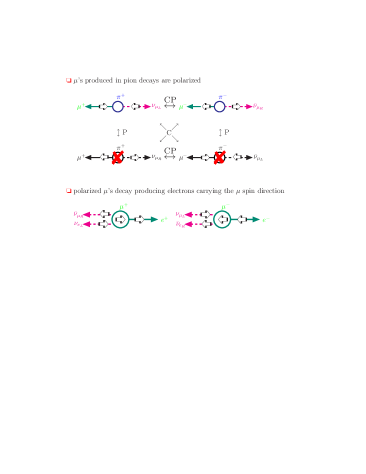
Figure 1: Spin transfer properties in production and decay of the muons (P=parity, C=charge conjugation). $\mu^{-}$ [$\mu^{+}$] is produced with positive [negative] helicity $h=\vec{s}\cdot\vec{p}/|\vec{p}|$, decay $e^{-}$ [$e^{+}$] have negative [positive] helicity, respectively

Note that the “maximal” parity ($P$) violation means that the charged weak transition currents only couple to left-handed neutrinos $\nu_{\mu\raisebox{-0.90417pt}{\tiny$L$}}$ and right-handed antineutrinos $\bar{\nu}_{\mu\raisebox{-0.90417pt}{\tiny$R$}}$, in other words, parity violation is a direct consequence of the fact that the neutrinos $\nu_{\mu\raisebox{-0.90417pt}{\tiny$R$}}$ and $\bar{\nu}_{\mu\raisebox{-0.90417pt}{\tiny$L$}}$ show no electromagnetic, weak and strong interaction in nature! as if they were non-existent.

2 The BNL Muon $g-2$ Experiment

After the proposal of parity violation in weak transitions by Lee and Yang in 1957, it immediately was realized that muons produced in weak decays of the pion ($\pi^{+}\to\mu^{+}+$ neutrino) should be longitudinally polarized. In addition, the decay positron of the muon ($\mu^{+}\to e^{+}+2$ neutrinos) could indicate the muon spin direction. This was confirmed by Garwin, Lederman and Weinrich 02Garwin57 and Friedman and Telegdi 02Friedman57 . The first of the two papers for the first time determined $g_{\mu}=2.00$ within 10% by applying the muon spin precession principle. Now the road was free to seriously think about the experimental investigation of $a_{\mu}$.

The first measurement of $(g_{\mu}-2)/2$ was performed at Columbia in 1960 02Columbia60 with a result $a_{\mu}=0.00122(8)$ at a precsision of about 5%. Soon later in 1961, at the CERN cyclotron (1958-1962) the first precision determination became available 02CERN62 . Surprisingly, nothing special was observed within the 0.4% level of accuracy of the experiment. It was the first real evidence that the muon was just a heavy electron. In particular this meant that the muon is point-like and no extra short distance effects could be seen. This latter point of course is a matter of accuracy and the challenge to go further was evident.

The idea of a muon storage ring was put forward next. A first one was successfully realized at CERN (1962-1968) 02CERN66 . It allowed to measure $a_{\mu}$ for both $\mu^{+}$ and $\mu^{-}$ at the same machine. Results agreed well within errors and provided a precise verification of the CPT theorem for muons. An accuracy of 270 ppm was reached and an insignificant 1.7 $\sigma$ (1 $\sigma$ = 1 standard deviation) deviation from theory was found. Nevertheless the latter triggered a reconsideration of theory. It turned out that in the estimate of the three-loop $O(\alpha^{3})$ QED contribution the leptonic “light-by-light scattering” part in the radiative corrections (dominated by the electron loop) was missing. Aldins et al. 02LBLlep69 then calculated this and after including it, perfect agreement between theory and experiment was obtained.

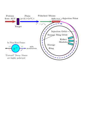
Figure 2: The schematics of muon injection and storage in the $g-2$ ring

The CERN muon $g-2$ experiment was shut down end of 1976, while data analysis continued until 1979 02Bailey79 . Only a few years later, in 1984 the E821collaboration formed, with the aim to perform a new experiment at Brookhaven National Laboratory (BNL). Data taking was between 1998 and 2001. The data analysis was completed in 2004. The E821 $g-2$ measurements achieved the remarkable precision of 0.54ppm 02BNL04 ; 02BNLfinal , which is a 14-fold improvement of the CERN result. The principle of the BNL muon $g-2$ experiments involves the study of the orbital and spin motion of highly polarized muons in a magnetic storage ring. This method has been applied in the last CERN experiment already. The key improvements of the BNL experiment include the very high intensity of the primary proton beam from the Alternating Gradient Synchrotron (AGS), the injection of muons instead of pions into the storage ring, and a superferric storage ring magnet. The protons hit a target and produce pions. The pions are unstable and decay into muons plus a neutrino where the muons carry spin and thus a magnetic moment which is directed along the direction of the flight axis. The longitudinally polarized muons from pion decay are then injected into a uniform magnetic field $\vec{B}$ where they travel in a circle (see Fig. 2).

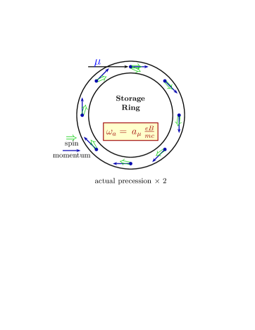
Figure 3: Spin precession in the $g-2$ ring ($\sim 12^{\circ}$/circle)

When polarized muons travel on a circular orbit in a constant magnetic field, as illustrated in Fig. 3, then $a_{\mu}$ is responsible for the Larmor precession of the direction of the spin of the muon, characterized by the angular fequency $\vec{\omega}_{a}$. At the magic energy of about $\sim$ 3.1 GeV, the latter is directly proportional to $a_{\mu}$:

$$\vec{\omega}_{a}=\frac{e}{m}\left[a_{\mu}\vec{B}-\left(a_{\mu}-\frac{1}{\gamma^{2}-1}\right)\>\vec{\beta}\times\vec{E}\right]_{{\mathrm{at}\;"\mathrm{magic}\ \gamma"}}^{E\sim 3.1\mathrm{GeV}}\simeq\frac{e}{m}\left[a_{\mu}\vec{B}\right]\;.$$ (9)

Electric quadrupole fields $\vec{E}$ are needed for focusing the beam and they affect the precession frequency in general. $\gamma=E/m_{\mu}=1/\sqrt{1-\beta^{2}}$ is the relativistic Lorentz factor with $\beta=v/c$ the velocity of the muon in units of the speed of light $c$. The magic energy $E_{\mathrm{mag}}=\gamma_{\mathrm{mag}}m_{\mu}$ is the energy $E$ for which $\frac{1}{\gamma_{\mathrm{mag}}^{2}-1}=a_{\mu}$. The existence of a solution is due to the fact that $a_{\mu}$ is a positive constant in competition with an energy dependent factor of opposite sign (as $\gamma\geq 1$). The second miracle, which is crucial for the feasibility of the experiment, is the fact that $\gamma_{\mathrm{mag}}=\sqrt{(1+a_{\mu})/a_{\mu}}\simeq 29.378$ is large enough to provide the time dilatation factor for the unstable muon boosting the life time $\tau_{\mu}\simeq 2.197\times 10^{-6}~{}\mathrm{sec}$ to $\tau_{\mathrm{in\>flight}}=\gamma\>\tau_{\mu}\simeq 6.454\times 10^{-5}~{}\mathrm{sec}$, which allows the muons, traveling at $v/c=0.99942\cdots$, to be stored in a ring of reasonable size (diameter $\sim$ 14 m).

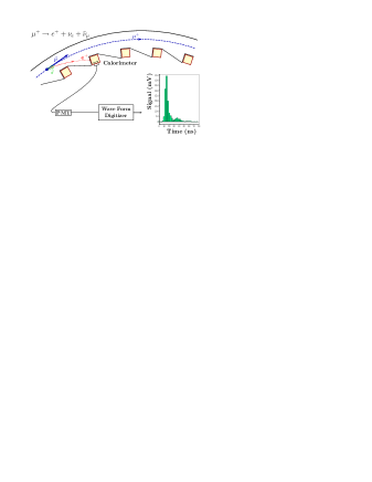
Figure 4: Decay of $\mu^{+}$ and detection of the emitted $e^{+}$ (PMT=Photomultiplier)

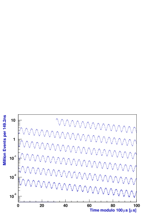
Figure 5: Distribution of counts versus time for the 3.6 billion decays in the 2001 negative muon data-taking period. Courtesy of the E821 collaboration 02BNL04

This provided the basic setup for the $g-2$ experiments at the muon storage rings at CERN and at BNL. The oscillation frequency $\vec{\omega}_{a}$ can be measured very precisely. Also the precise tuning to the magic energy is not the major problem. The most serious challenge is to manufacture a precisely known constant magnetic field $B$, as the latter directly enters the experimental extraction of $a_{\mu}$ (9). Of course one also needs high enough statistics to get sharp values for the oscillation frequency. The basic principle of the measurement of $a_{\mu}$ is a measurement of the “anomalous” frequency difference $\omega_{a}=|\vec{\omega}_{a}|=\omega_{s}-\omega_{c}$, where $\omega_{s}=g_{\mu}\>(e\hbar/2m_{\mu})\>B/\hbar=g_{\mu}/2\>\cdot~{}e/m_{\mu}\>B$ is the muon spin–flip precession frequency in the applied magnetic field and $\omega_{c}=e/m_{\mu}\>B$ is the muon cyclotron frequency. The principle of measuring $\omega_{a}$ is indicated in Fig. 4 and an example of a measured count spectrum is shown in Fig. 5. Instead of eliminating the magnetic field by measuring $\omega_{c}$, $B$ is determined from proton nuclear-magnetic-resonance (NMR) measurements. This procedure requires the value of $\mu_{\mu}/\mu_{p}$ to extract $a_{\mu}$ from the data. Fortunately, a high precision value for this ratio is available from the measurement of the hyperfine structure in muonium. One obtains

$$a_{\mu}=\frac{\bar{R}}{|\mu_{\mu}/\mu_{p}|-\bar{R}}\;,$$ (10)

where $\bar{R}=\omega_{a}/\bar{\omega}_{p}$ and $\bar{\omega}_{p}=(e/m_{\mu}c)\langle B\rangle$ is the free-proton NMR frequency corresponding to the average magnetic field, seen by the muons in their orbits in the storage ring. We mention that for the electron a Penning trap is employed to measure $a_{e}$ rather than a storage ring. The $B$ field in this case can be eliminated via a measurement of the cyclotron frequency. The BNL g-2 muon storage ring is shown in Fig. 6.

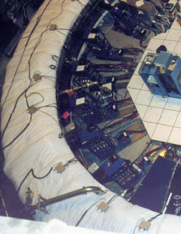
Figure 6: The Brookhaven National Laboratory muon storage ring. The ring has a radius of 7.112 meters, the aperture of the beam pipe is 90 mm, the field is 1.45 Tesla and the momentum of the muon is $p_{\mu}=3.094$ GeV/c. Picture taken from the Muon $g-2$ Collaboration Web Page http://www.g-2.bnl.gov/ (Courtesy of Brookhaven National Laboratory)

Since the spin precession frequency can be measured very well, the precision at which $g-2$ can be measured is essentially determined by the possibility to manufacture a constant homogeneous magnetic field $\vec{B}$. Important but easier to achieve is the tuning to the magic energy. The outcome of the experiment will be discussed later.

3 QED Prediction of $a_{e}$ and the Determination of $\alpha$

The anomalous magnetic moment $a_{\ell}$ is a dimensionless quantity, just a number, and corresponds to an effective tensor interaction term

$$\delta{\cal L}_{\mathrm{eff}}^{\mathrm{AMM}}=-\frac{e_{\ell}a_{\ell}}{4m_{\ell}}\>\bar{\psi}(x)\>\sigma^{\mu\nu}\>F_{\mu\nu}(x)\>\psi(x)\;,$$ (11)

which in an external magnetic field at low energy takes the well known form of a magnetic energy (up to a sign)

$$\delta{\cal L}_{\mathrm{eff}}^{\mathrm{AMM}}\Rightarrow-{\cal H}_{m}\simeq-\frac{e_{\ell}a_{\ell}}{2m_{\ell}}\>\vec{\sigma}\vec{B}\;.$$ (12)

Such a term, if present in the fundamental Lagrangian, would spoil renormalizability of the theory and contribute to $F_{\rm M}(q^{2})$ at the tree level. In addition, it is not $SU(2)_{L}$ gauge invariant, because gauge invariance only allows minimal couplings via a covariant derivative, i.e., vector and/or axial-vector terms. The emergence of an anomalous magnetic moment term in the SM is a consequence of the symmetry breaking by the Higgs mechanism, which provides the mass to the physical particles and allows for helicity flip processes like the anomalous magnetic moment transitions. In any renormalizable theory the anomalous magnetic moment term must vanish at tree level. This means that there is no free adjustable parameter associated with it. It is a finite prediction of the theory.

The reason why it is so interesting to have such a precise measurement of $a_{e}$ or $a_{\mu}$, of course, is that it can be calculated with comparable accuracy in theory by a perturbative expansion in $\alpha$ of the form

$$a_{\ell}\simeq\sum_{n=1}^{N}A^{(2n)}(\alpha/\pi)^{n}\;,$$ (13)

with up to $N=5$ terms under consideration at present. The experimental precision of $a_{e}$ (0.66 ppb) requires the knowledge of the coefficients with accuracies $\delta A^{(4)}\sim 1\times 10^{-7}$, $\delta A^{(6)}\sim 6\times 10^{-5}$, $\delta A^{(8)}\sim 2\times 10^{-2}$ and $\delta A^{(10)}\sim 10$. The expansion (13) is an expansion in the number $N$ of closed loops of the contributing Feynman diagrams.

The recent new determination of $a_{e}$ 02aenew allows for a very precise determination of the fine structure constant 02alnew ; 02Aoyama07

$$\alpha^{-1}(a_{e}) = 137.035999069(96)[0.70\mathrm{ppb}]\;,$$ (14)

which we will use in the evaluation of $a_{\mu}$.

At two and more loops results depend on lepton mass ratios. For the evaluation of these contributions precise values for the lepton masses are needed. We will use the following values for the muon–electron mass ratio, the muon and the tau mass 02PDG04 ; 02CODATA02

$$\begin{array}[]{c}m_{\mu}/m_{e}=206.768\,2838\,(54)~{},~{}~{}m_{\mu}/m_{\tau}=0.059\,4592\,(97)\\ m_{e}=0.510\,9989\,918(44)\mathrm{MeV}~{},~{}~{}m_{\mu}=105.658\,3692\,(94)\mathrm{MeV}\\ m_{\tau}=1776.99\,(29)\mathrm{MeV}\;.\end{array}$$ (18)

The leading contributions to $a_{\ell}$ can be calculated in QED. With increasing precision higher and higher terms become relevant. At present, 4–loops are indispensable and strong interaction effects like hadronic vacuum polarization (vap) or hadronic light-by-light scattering (lbl) as well as weak effects have to be considered. Typically, analytic results for higher order terms may be expressed in terms of the Riemann zeta function

$$\zeta(n)=\sum\limits_{k=1}^{\infty}\frac{1}{k^{n}}$$ (19)

and of the poly-logarithmic integrals

$$\mathrm{Li}_{n}(x)=\frac{(-1)^{n-1}}{(n-2)!}\int\limits_{0}^{1}\frac{\ln^{n-2}(t)\ln(1-tx)}{t}dt=\sum\limits_{k=1}^{\infty}\frac{x^{k}}{k^{n}}\;.$$ (20)

We first discuss the universal contributions $a_{\ell}$ in “one flavor QED”, with one type of lepton lines only. At leading order one has
$\bullet$ one 1-loop diagram

1

giving the result mentioned before.

$\bullet$ At 2-loops 7 diagrams with only $\ell$-type fermion lines

0.75 1

which contribute a term

$$a_{\ell}^{(4)}=\left[\frac{197}{144}+\frac{\pi^{2}}{12}-\frac{\pi^{2}}{2}\ln 2+\frac{3}{4}\zeta(3)\right]\>\left(\frac{\alpha}{\pi}\right)^{2}\;,$$ (21)

obtained independently by Peterman 02Petermann57 and Sommerfield 02Sommerfield57 in 1957.

$\bullet$ At 3-loops, with one type of fermion lines only, the 72 diagrams of Fig. 7 contribute. Most remarkably, after about 25 years of hard work, Laporta and Remiddi in 1996 02LaportaRemiddi96 managed to give a complete analytic result (see also 02Remiddietal69-95 )

$$a_{\ell}^{(6)} = \left[\frac{28259}{5184}+\frac{17101}{810}\pi^{2}-\frac{298}{9}\pi^{2}\ln 2+\frac{139}{18}\zeta(3)+\frac{100}{3}\left\{\mathrm{Li}_{4}(\frac{1}{2})+\frac{1}{24}\ln^{4}2\right.\right.$$ (22)

$$\left.\left.-\frac{1}{24}\pi^{2}\ln^{2}2\right\}-\frac{239}{2160}\pi^{4}+\frac{83}{72}\pi^{2}\zeta(3)-\frac{215}{24}\zeta(5)\right]\>\left(\frac{\alpha}{\pi}\right)^{3}\;.$$

This result was confirming Kinoshita’s earlier numerical evaluation 02Ki95 .

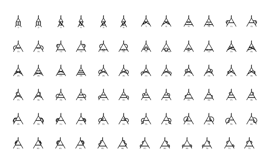
Figure 7: The universal third order contribution to $a_{\mu}$. All fermion loops here are muon–loops (first 22 diagrams). All non-universal contributions follow by replacing at least one muon in a closed loop by some other fermion

The big advantage of the analytic result is that it allows a numerical evaluation at any desired precision. The direct numerical evaluation of the multidimensional Feynman integrals by Monte Carlo methods is always of limited precision and an improvement is always very expensive in computing power.

$\bullet$ At 4-loops 891 diagrams contribute to the universal term. Their evaluation is possible by numerical integration and has been performed in a heroic effort by Kinoshita 02KiLi83-89 (reviewed in 02HuKi99 ), and was updated recently by Kinoshita and his collaborators (2002/2005/2007) 02KiNi05 ; 02Aoyama07 .

The largest uncertainty comes from 518 diagrams without fermion loops contributing to the universal term $A^{(8)}_{1}$. Completely unknown is the universal five–loop term $A^{(10)}_{1}$, which is leading for $a_{e}$. An estimation discussed in 02CODATA05 suggests that the 5-loop coefficient has at most a magnitude of 3.8. We adopt this estimate and take into account $A^{(10)}_{1}=0.0(3.8)$ (as in 02KiNi05 ).

Collecting the universal terms we have

$$a_{\ell}^{\rm uni} = 0.5\>\left(\frac{\alpha}{\pi}\right)-0.32847896557919378\ldots\>\left(\frac{\alpha}{\pi}\right)^{2}$$ (23)

$$+1.181241456587\ldots\>\left(\frac{\alpha}{\pi}\right)^{3}-1.9144(35)\>\left(\frac{\alpha}{\pi}\right)^{4}+0.0(3.8)\>\left(\frac{\alpha}{\pi}\right)^{5}$$

$$= 0.001\,159\,652\,176\,42(81)(10)(26)[86]\cdots$$

for the one–flavor QED contribution. The three errors are: the error of $\alpha$, given in (14), the numerical uncertainty of the $\alpha^{4}$ coefficient and the estimated size of the missing higher order terms, respectively.

At two loops and higher, internal fermion-loops show up, where the flavor of the internal fermion differs form the one of the external lepton, in general. As all fermions have different masses, the fermion-loops give rise to mass dependent effects, which were calculated at two-loops in 02SWP57 ; 02El66 (see also 02LdeR69 ; 02Lautrup77 ; 02LdeR74 ; 02LiMeSa93 ), and at three-loops in 02Ki67 ; 02A26early ; 02SaLi91 ; 02La93 ; 02LR93 ; 02KOPV03 .

The leading mass dependent effects come from photon vacuum polarization, which leads to charge screening. Including a factor $e^{2}$ and considering the renormalized photon propagator (wave function renormalization factor $Z_{\gamma}$) we have

$${\rm i}\>e^{2}\>D^{{}^{\prime}\mu\nu}_{\gamma}(q)=\frac{-{\rm i}g^{\mu\nu}\>e^{2}\>Z_{\gamma}}{q^{2}\>\left(1+\Pi^{\prime}_{\gamma}(q^{2})\right)}+{\rm\ gauge\ terms\ }$$ (24)

which in effect means that the charge has to be replaced by an energy-momentum scale dependent running charge

$$e^{2}\to e^{2}(q^{2})=\frac{e^{2}Z_{\gamma}}{1+\Pi^{\prime}_{\gamma}(q^{2})}\;.$$ (25)

The wave function renormalization factor $Z_{\gamma}$ is fixed by the condition that as $q^{2}\to 0$ one obtains the classical charge (charge renormalization in the Thomson limit). Thus the renormalized charge is

$$e^{2}\to e^{2}(q^{2})=\frac{e^{2}}{1+(\Pi^{\prime}_{\gamma}(q^{2})-\Pi^{\prime}_{\gamma}(0))}$$ (26)

where in perturbation theory the lowest order diagram which contributes to $\Pi^{\prime}_{\gamma}(q^{2})$ is

and describes the virtual creation and re-absorption of fermion pairs $\gamma^{*}\rightarrow e^{+}e^{-},\mu^{+}\mu^{-},\tau^{+}\tau^{-},u\bar{u},d\bar{d},$ $\cdots(\mathrm{had})\rightarrow~{}~{}\gamma^{*}$ .

In terms of the fine structure constant $\alpha=\frac{e^{2}}{4\pi}$ Eq. (26) reads

$$\alpha(q^{2})=\frac{\alpha}{1-\Delta\alpha(q^{2})}\;\;\;;\;\;\;\Delta\alpha(q^{2})=-{\rm Re}\>\left(\Pi^{\prime}_{\gamma}(q^{2})-\Pi^{\prime}_{\gamma}(0)\right)\;.$$ (27)

The various contributions to the shift in the fine structure constant come from the leptons (lep = $e$, $\mu$ and $\tau$), the 5 light quarks ($u$, $b$, $s$, $c$, and $b$) and/or the corresponding hadrons (had). The top quark is too heavy to give a relevant contribution. The hadronic contributions will be considered later. The running of $\alpha$ is governed by the renormalization group (RG). In the context of $g-2$ calculations, the use of RG methods has been advocated in 02LdeR74 . In fact, the enhanced short-distance logarithms may be obtained by the substitution $\alpha\to\alpha(m_{\mu})=\alpha\>(1+\frac{2}{3}\frac{\alpha}{\pi}\>\ln\frac{m_{\mu}}{m_{e}}+\cdots)$ in a lower order result (see the following example).

Typical contributions are the following:
$-$ LIGHT internal masses give rise to log’s of mass ratios which become singular in the light mass to zero limit (logarithmically enhanced corrections)
2

$-$ HEAVY internal masses decouple, i.e., they give no effect in the heavy mass to infinity limit
1

New physics contributions from states which are too heavy to be produced at present accelerator energies typically give this kind of contribution. Even so $a_{\mu}$ is 786 times less precise than $a_{e}$ it is still 54 times more sensitive to new physics (NP).

Corrections due to internal $e$, $\mu$- and $\tau$-loops are different for $a_{e}$, $a_{\mu}$ and $a_{\tau}$. For reasons of comparison and because of its role in the precise determination of $\alpha$ we briefly consider $a_{e}$ first. The result is of the form

$$a_{e}^{\mathrm{QED}}=a_{e}^{\rm uni}+a_{e}(\mu)+a_{e}(\tau)+e_{e}(\mu,\tau)$$ (28)

with 02El66 ; 02La93 ; 02LR93

$$a_{e}(\mu) = 5.197\,386\,70(27)\times 10^{-7}{\left(\frac{\alpha}{\pi}\right)^{2}}-7.373\,941\,64(29)\times 10^{-6}{\left(\frac{\alpha}{\pi}\right)^{3}}$$

$$a_{e}(\tau) = 1.83763(60)\times 10^{-9}{\left(\frac{\alpha}{\pi}\right)^{2}}-6.5819(19)\times 10^{-8}{\left(\frac{\alpha}{\pi}\right)^{3}}$$

$$a_{e}(\mu,\tau) = 0.190945(62)\times 10^{-12}{\left(\frac{\alpha}{\pi}\right)^{3}}\;.$$

The QED part thus may be summarized in the prediction

$$a_{e}^{\rm QED} = \frac{\alpha}{2\pi}-0.328\,478\,444\,002\,90(60)\left(\frac{\alpha}{\pi}\right)^{2}$$ (29)

$$+1.181\,234\,016\,828(19)\left(\frac{\alpha}{\pi}\right)^{3}-1.9144(35)\left(\frac{\alpha}{\pi}\right)^{4}+0.0(3.8)\left(\frac{\alpha}{\pi}\right)^{5}.$$

The hadronic and weak contributions to $a_{e}$ are small : $a_{e}^{\rm had}=1.67(3)\times 10^{-12}$ and $a_{e}^{\rm weak}=0.036\times 10^{-12}$, respectively. The hadronic contribution now just starts to be significant, however, unlike in $a_{\mu}^{\rm had}$ for the muon, $a_{e}^{\rm had}$ is known with sufficient accuracy and is not the limiting factor here. The theory error is dominated by the missing 5-loop QED term. As a result $a_{e}$ essentially only depends on perturbative QED, while hadronic, weak and new physics (NP) contributions are suppressed by $(m_{e}/M)^{2}$, where $M$ is a weak, hadronic or new physics scale. As a consequence $a_{e}$ at this level of accuracy is theoretically well under control (almost a pure QED object) and therefore is an excellent observable for extracting $\alpha_{\rm QED}$ based on the SM prediction

$$a_{e}^{\rm SM} = a_{e}^{\rm QED}\mathrm{[Eq.~{}(\ref{02aeQED})]}+1.706(30)\times 10^{-12}~{}~{}\mbox{(hadronic \& weak)}\;.$$ (30)

We now compare this result with the very recent extraordinary precise measurement of the electron anomalous magnetic moment 02aenew

$$a_{e}^{\rm exp}=0.001\,159\,652\,180\,85(76)$$ (31)

which yields

$$\alpha^{-1}(a_{e}) = 137.035999069(90)(12)(30)(3)\;,$$

which is the value (14) 02alnew ; 02Aoyama07 we use in calculating $a_{\mu}$. The first error is the experimental one of $a_{e}^{\mathrm{exp}}$, the second and third are the numerical uncertainties of the $\alpha^{4}$ and $\alpha^{5}$ terms, respectively. The last one is the hadronic uncertainty, which is completely negligible. Note that the largest theoretical uncertainty comes from the almost completely missing information concerning the 5–loop contribution. This is now the by far most precise determination of $\alpha$ and we will use it throughout in the calculation of $a_{\mu}$, below.
The best determinations of $\alpha$ which do not depend on $a_{e}$ are 02Cs06 ; 02Rb06

$$\alpha^{-1}(\mathrm{Cs06}) = 137.03600000(110)[8.0\,\mathrm{ppb}]\;,$$

$$\alpha^{-1}(\mathrm{Rb06}) = 137.03599884(091)[6.7\,\mathrm{ppb}]\;,$$

less precise by about a factor ten. $\alpha(\mathrm{Cs06})$ is determined from a measurement of $h/M_{\mathrm{Cs}}$ via Cesium recoil measurements 02Cs06 , while $\alpha(\mathrm{Rb06})$ derives from the ratio $h/M_{\mathrm{Rb}}$ measured via Bloch oscillations of Rubidium atoms in an optical lattice 02Rb06 . These values should be used in theoretical predictions of $a_{e}$. Using $\alpha(\mathrm{Cs06})$ we get $a_{e}=0.00115965217298(930)$ and $a_{e}^{\mathrm{exp}}-a_{e}^{\mathrm{the}}=7.87(9.33)\times 10^{-12}$, with $\alpha(\mathrm{Rb06})$ the prediction reads $a_{e}=0.00115965218279(769)$ and $a_{e}^{\mathrm{exp}}-a_{e}^{\mathrm{the}}=-1.94(7.73)\times 10^{-12}$ in best agreement. The error of the prediction is completely dominated by the uncertainty coming from $\alpha(\mathrm{Cs06})$ and $\alpha(\mathrm{Rb06})$ such that an improvement of $\alpha$ by a factor 10 would allow a much more stringent test of QED (see also 02alnew ; 02Aoyama07 ). If one assumes that $\left|\Delta a_{e}^{\rm New\ Physics}\right|\simeq m_{e}^{2}/\Lambda^{2}$ where $\Lambda$ approximates the scale of “New Physics”, then the agreement between $\alpha^{-1}(a_{e})$ and $\alpha^{-1}(\mathrm{Rb06})$ currently probes $\Lambda\mbox{\raisebox{-1.03334pt}{\footnotesize$\>\stackrel{{\scriptstyle<}}{{\sim}}\>$}}O(\mbox{250 GeV})$. To access the much more interesting $\Lambda\sim O(\mbox{1 TeV})$ region also a bigger effort on the theory side would by necessary about the $O(\alpha^{4})$ and the $O(\alpha^{5})$ terms.

4 Standard Model Prediction for $a_{\mu}$

4.1 QED Contribution

The SM prediction of $a_{\mu}$ looks formally very similar to the one for $a_{e}$, however, besides the common universal part, the mass dependent, the hadronic and the weak effects enter with very different weight and significance. The mass-dependent QED corrections follow from the universal set of diagrams (see e.g. Fig. 7 for the 3 loop case) by replacing the closed internal $\mu$–loops by $e$– and/or $\tau$–loops. Typical contributions come from vacuum polarization or light-by-light scattering loops, like

The result is given by

$$a_{\mu}=a_{e}^{\rm uni}+a_{\mu}(m_{\mu}/m_{e})+a_{\mu}(m_{\mu}/m_{\tau})+a_{\mu}(m_{\mu}/m_{e},m_{\mu}/m_{\tau})$$ (32)

with 02El66 ; 02La93 ; 02LR93 ; 02KOPV03

$$a_{\mu}(m_{\mu}/m_{e}) = 1.094~{}258~{}311~{}1~{}(84)\>{\left(\frac{\alpha}{\pi}\right)^{2}}+22.868~{}380~{}02~{}(20)~{}\>{\left(\frac{\alpha}{\pi}\right)^{3}}$$

$$+~{}~{}132.682~{}3~{}(72)~{}~{}\>{\left(\frac{\alpha}{\pi}\right)^{4}}$$

$$a_{\mu}(m_{\mu}/m_{\tau}) = 7.8064~{}(25)\times 10^{-5}~{}\>{\left(\frac{\alpha}{\pi}\right)^{2}}+36.051~{}(21)\times 10^{-5}\>{\left(\frac{\alpha}{\pi}\right)^{3}}$$

$$+~{}~{}~{}~{}~{}0.005~{}(3)~{}~{}~{}\>{\left(\frac{\alpha}{\pi}\right)^{4}}$$

$$a_{\mu}(m_{\mu}/m_{e},m_{\mu}/m_{\tau}) = 52.766~{}(17)\times 10^{-5}\>{\left(\frac{\alpha}{\pi}\right)^{3}}+~{}~{}0.037~{}594~{}(83)\>{\left(\frac{\alpha}{\pi}\right)^{4}}$$

except for the last term, which has been worked out as a series expansion in the mass ratios 02CS99 ; 02FGdR05 , all contributions are known analytically in exact form 02La93 ; 02LR93 up to 3–loops. At 4–loops only a few terms are known analytically 02A8analytic . Again the relevant 4–loop contributions have been evaluated by numerical integration methods by Kinoshita and Nio 02KiNi04 . The 5–loop term has been estimated to be $A^{(10)}_{2}(m_{\mu}/m_{e})=663(2)$ in 02Ka93 ; 02KiNi06 ; 02Kataev05 .

Our knowledge of the QED result for $a_{\mu}$ may be summarized by

$$a_{\mu}^{\rm QED} = \frac{\alpha}{2\pi}+0.765\,857\,410(26)\left(\frac{\alpha}{\pi}\right)^{2}$$ (33)

$$+24.050\,509\,65(46)\left(\frac{\alpha}{\pi}\right)^{3}+130.8105(85)\left(\frac{\alpha}{\pi}\right)^{4}+663(20)\left(\frac{\alpha}{\pi}\right)^{5}.$$

Growing coefficients in the $\alpha/\pi$ expansion reflect the presence of large $\ln\frac{m_{\mu}}{m_{e}}\simeq 5.3$ terms coming from electron loops. In spite of the strongly growing expansion coefficients the convergence of the perturbation series is excellent

# n of loops	$C_{i}$ [$(\alpha/\pi)^{n}$]		$a_{\mu}^{\rm QED}\times 10^{11}~{}~{}~{}~{}~{}$
1	+0.	5	116140973.30 (0.08)
2	+0.	765 857 410(26)	413217.62 (0.01)
3	+24.	050 509 65(46)	30141.90 (0.00)
4	+130.	8105(85)	380.81 (0.03)
5	+663.	0(20.0)	4.48 (0.14)
tot			116584718.11 (0.16)

because $\alpha/\pi$ is a truly small expansion parameter.

The different higher order QED contributions are collected in Tab. 1. We thus arrive at a QED prediction of $a_{\mu}$ given by

Table 1: QED contributions to $a_{\mu}$ in units $10^{-6}$

term	universal		$e$–loops		$\tau$–loops		$e$&$\tau$–loops
$a^{(4)}$	$\,-1$.	$772\,305\,06~{}(0)$	$\,5$.	$904\,060\,07~{}~{}(5)$	$\,0$.	$000\,421\,20(13)$	$-$
$a^{(6)}$	$0$.	$014\,804\,20~{}(0)$	$0$.	$286\,603\,69~{}~{}(0)$	$0$.	$000\,004\,52~{}(1)$	$\,0$.	$000\,006\,61(0)$
$a^{(8)}$	$-0$.	$000\,055\,73(10)$	$0$.	$003\,862\,56~{}(21)$	$0$.	$000\,000\,15~{}(9)$	$0$.	$000\,001\,09(0)$
$a^{(10)}$	$0$.	$000\,000\,00(26)$	$0$.	$000\,044\,83(135)$	?		?

$$a_{\mu}^{\mathrm{QED}}=116\,584\,718.113(.082)(.014)(.025)(.137)[.162]\times 10^{-11}$$ (34)

where the first error is the uncertainty of $\alpha$ in (14), the second one combines in quadrature the uncertainties due to the errors in the mass ratios, the third is due to the numerical uncertainty and the last stands for the missing $O(\alpha^{5})$ terms. With the new value of $\alpha[a_{e}]$ the combined error is dominated by our limited knowledge of the 5–loop term.

4.2 Weak Contributions

The electroweak SM is a non-Abelian gauge theory with gauge group $SU(2)_{L}\otimes U(1)_{Y}\to U(1)_{\mathrm{QED}}$, which is broken down to the electromagnetic Abelian subgroup $U(1)_{\mathrm{QED}}$ by the Higgs mechanism, which requires a scalar Higgs field $H$ which receives a vacuum expectation value $v$. The latter fixes the experimentally well known Fermi constant $G_{\mu}=1/(\sqrt{2}v^{2})$ and induces the masses of the heavy gauge bosons $M_{W}$ and $M_{Z}$ as well as all fermion masses $m_{f}$. Other physical constants which we will need later for evaluating the weak contributions are the Fermi constant

$$G_{\mu}=1.16637(1)\times 10^{-5}~{}~{}~{}\mathrm{GeV}^{-2}\;,$$ (35)

the weak mixing parameter

$$\sin^{2}\Theta_{W}=0.22276(56)$$ (36)

and the masses of the intermediate gauge bosons $Z$ and $W$

$$M_{Z}=91.1876\pm 0.0021\ \mathrm{GeV}\;,M_{W}=80.392\pm 0.029\ \mathrm{GeV}\;.$$ (37)

For the not yet discovered SM Higgs particle the mass is constrained by LEP data to the range

$$114\ \mathrm{GeV}<m_{H}<200\ \mathrm{GeV\ }(\mathrm{at\ }96\%\mathrm{\ CL})\;.$$ (38)

The weak interaction contributions to $a_{\mu}$ are due to the exchange of the heavy gauge bosons, the charged $W^{\pm}$ and the neutral $Z$, which mixes with the photon via a rotation by the weak mixing angle $\Theta_{W}$ and which defines the weak mixing parameter $\sin^{2}\Theta_{W}=1-M_{W}^{2}/M_{Z}^{2}$. What is most interesting is the occurrence of the first diagram of Fig. 8, which exhibits a non-Abelian triple gauge vertex and the corresponding contribution provides a test of the Yang–Mills structure involved. It is of course not surprising that the photon couples to the charged $W$ boson the way it is dictated by electromagnetic gauge invariance.

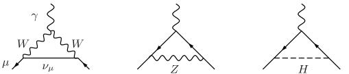
Figure 8: The leading weak contributions to $a_{\ell}$; diagrams in the physical unitary gauge

The gauge boson contributions up to negligible terms of order $O(\frac{m_{\mu}^{2}}{M_{W,Z}^{2}})$ are given by 02EW1Loop

$$a^{(2)\>\mathrm{EW}}_{\mu}(W) = \frac{\sqrt{2}G_{\mu}m_{\mu}^{2}}{16\pi^{2}}\>\frac{10}{3}\simeq+388.70(0)\times 10^{-11}$$

$$a^{(2)\>\mathrm{EW}}_{\mu}(Z) = \frac{\sqrt{2}G_{\mu}m_{\mu}^{2}}{16\pi^{2}}\>\frac{(-1+4\>\sin^{2}\Theta_{W})^{2}-5}{3}\simeq-193.88(2)\times 10^{-11}$$

while the diagram with the Higgs exchange, for $m_{H}\gg m_{\mu}$, yields

$$a^{(2)\>\mathrm{EW}}_{\mu}(H) \simeq \frac{\sqrt{2}G_{\mu}m_{\mu}^{2}}{4\pi^{2}}\>\frac{m_{\mu}^{2}}{m_{H}^{2}}\>\ln\frac{m_{\mu}^{2}}{m_{H}^{2}}+\cdots\leq 5\times 10^{-14}~{}~{}\mathrm{for}~{}~{}m_{H}\geq 114~{}\mathrm{GeV}\;.$$

Employing the SM parameters given in (35) and (36) we obtain

$$a_{\mu}^{(2)\>\mathrm{EW}}=(194.82\pm 0.02)\times 10^{-11}$$ (39)

The error comes from the uncertainty in $\sin^{2}\Theta_{W}$ given above.

The electroweak two–loop corrections have to be taken into account as well. In fact triangle fermion–loops may give rise to unexpectedly large radiative corrections. The diagrams which yield the leading corrections are those including a VVA triangular fermion–loop ($VVA\neq 0$ while $VVV=0$) associated with a $Z$ boson exchange

which exhibits a parity violating axial coupling (A). A fermion of flavor $f$ yields a contribution

$$a^{(4)\>\mathrm{EW}}_{\mu}([f])\simeq\frac{\sqrt{2}G_{\mu}m_{\mu}^{2}}{16\pi^{2}}\frac{\alpha}{\pi}\>2T_{3f}N_{cf}Q_{f}^{2}\>\left[3\ln\frac{M_{Z}^{2}}{m_{f^{\prime}}^{2}}+C_{f}\right]$$ (40)

where $T_{3f}$ is the 3rd component of the weak isospin, $Q_{f}$ the charge and $N_{cf}$ the color factor, 1 for leptons, 3 for quarks. The mass $m_{f^{\prime}}$ is $m_{\mu}$ if $m_{f}<m_{\mu}$ and $m_{f}$ if $m_{f}>m_{\mu}$, and $C_{e}=5/2,~{}C_{\mu}=11/6-8/9\>\pi^{2},~{}C_{\tau}=-6$ 02KKSS92 . However, in the SM the consideration of individual fermions makes no sense and a separation of quarks and leptons is not possible. Mathematical consistency of the SM requires complete VVA anomaly cancellation between leptons and quarks, and actually $\sum_{f}N_{cf}Q_{f}^{2}T_{3f}=0$ holds for each of the 3 known lepton–quark families separately. Treating, in a first step, the quarks like free fermions (quark parton model QPM) the first two families yield (using $m_{u}=m_{d}=300~{}\mathrm{MeV}\;,m_{s}=500~{}\mathrm{MeV}\;,m_{c}=1.5\mathrm{GeV}$)

$$a_{\mu}^{(4)\>\mathrm{EW}}(\left[\begin{tabular}[]{c}$e,u,d$\\ $\mu,c,s$\end{tabular}\right])_{\mathrm{QPM}} \simeq -\frac{\sqrt{2}G_{\mu}\>m_{\mu}^{2}}{16\pi^{2}}\>\frac{\alpha}{\pi}\>\left[\ln\frac{m_{u}^{8}m_{c}^{8}}{m_{\mu}^{12}m_{d}^{2}m_{s}^{2}}+\frac{49}{3}-\frac{8\pi^{2}}{9}\right]$$ (44)

$$\simeq-\frac{\sqrt{2}G_{\mu}\>m_{\mu}^{2}}{16\pi^{2}}\>\frac{\alpha}{\pi}\>\times 32.0(?)\simeq-8.65(?)\times 10^{-11}\;,$$

which demonstrates that the leading large logs $\sim\ln M_{Z}$ have canceled 02CKM95F , as it should be. However, the quark masses which appear here are ill-defined constituent quark masses, which can hardly account reliably for the strong interaction effects, therefore the question marks in place of the errors.

In fact, low energy QCD is characterized in the chiral limit of massless light quarks $u,d,s$, by spontaneous chiral symmetry breaking (S$\chi$SB) of the chiral group $SU(3)_{V}\otimes SU(3)_{A}$, which in particular implies the existence of the pseudoscalar octet of pions and kaons as Goldstone bosons. The light quark condensates are essential features in this situation and lead to non-perturbative effects completely absent in a perturbative approach. Thus low energy QCD effects are intrinsically non–perturbative and controlled by chiral perturbation theory (CHPT), the systematic QCD low energy expansion, which accounts for the S$\chi$SB and the chiral symmetry breaking by quark masses in a systematic manner. The low energy effective theory describing the hadronic contributions related to the light quarks $u,d,s$ requires the calculation of the diagrams of the type shown in Fig. 9.

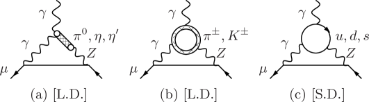
Figure 9: The two leading CHPT diagrams (L.D.) and the QPM diagram (S.D.). The charged pion loop is sub-leading and is discarded. Diagrams with permuted $\gamma\leftrightarrow Z$ on the $\mu$-line have to be included

The leading effect for the 1st plus 2nd family takes the form 02PPdeR95

$$a_{\mu}^{(4)\>\mathrm{EW}}(\left[\begin{tabular}[]{c}$e,u,d$\\ $\mu,c,s$\end{tabular}\right])_{\mathrm{CHPT}} = \frac{\sqrt{2}G_{\mu}\>m_{\mu}^{2}}{16\pi^{2}}\>\frac{\alpha}{\pi}\>\left[-\frac{14}{3}\ln\frac{M_{\Lambda}^{2}}{m_{\mu}^{2}}+4\ln\frac{M_{\Lambda}^{2}}{m_{c}^{2}}-\frac{35}{3}+\frac{8}{9}\pi^{2}\right]$$ (48)

$$\simeq-\frac{\sqrt{2}G_{\mu}\>m_{\mu}^{2}}{16\pi^{2}}\>\frac{\alpha}{\pi}\>\times 26.2(5)\simeq-7.09(13)\times 10^{-11}\;.$$

The error comes from varying the cut–off $M_{\Lambda}$ between 1 GeV and 2 GeV. Below 1 GeV CHPT can be trusted above 2 GeV we can trust pQCD. Fortunately the result is not very sensitive to the choice of the cut–off. For more sophisticated analyses we refer to 02CKM95F ; 02PPdeR95 ; 02KPPdeR02 which was corrected and refined in 02DG98 ; 02CMV03 . Thereby, a new kind of non-renormalization theorems played a key role 02Vainshtein03 ; 02KPPdR04 ; 02JT05 . Including subleading effects yields $-6.7\times 10^{-11}$ for the first two families. The 3rd family of fermions including the heavy top quark can be treated in perturbation theory and has been worked out to be $-8.2\times 10^{-11}$ in 02D'Hoker92 . Subleading fermion loops contribute $-5.3\times 10^{-11}$. There are many more diagrams contributing, in particular the calculation of the bosonic contributions (1678 diagrams) is a formidable task and has been performed 1996 by Czarnecki, Krause and Marciano as an expansion in $(m_{\mu}/M_{V})^{2}$ and $(M_{V}/m_{H})^{2}$ 02CKM96B . Later complete calculations, valid also for lighter Higgs masses, were performed 02HSW04 ; 02GC05 , which confirmed the previous result $-22.3\times 10^{-11}$. The 3rd family of fermions including the heavy top quark can be treated in perturbation theory and has been worked out in 02D'Hoker92 .

The complete weak contribution may be summarized by 02CMV03

$$a_{\mu}^{\mathrm{EW}} = \frac{\sqrt{2}G_{\mu}\>m_{\mu}^{2}}{16\pi^{2}}\>\left\{\frac{5}{3}+\frac{1}{3}\>(1-4\sin^{2}\Theta_{W})^{2}-\frac{\alpha}{\pi}[155.5(4)(2)]\right\}$$ (49)

$$= (154\pm 1[\rm had]\pm 2[m_{H},m_{t},3-loop])\times 10^{-11}$$

with errors from triangle quark loops and from variation of the Higgs mass in the range $m_{H}=150^{+100}_{-40}$ GeV. The 3-loop effect has been estimated to be negligible 02DG98 ; 02CMV03 .

4.3 Hadronic Contributions

So far when we were talking about fermion loops we only considered the lepton loops. Besides the leptons also the strongly interacting quarks have to be taken into account. The problem is that strong interactions at low energy are non-perturbative and straight forward first principle calculations become very difficult and often impossible.

Fortunately the leading hadronic effects are vacuum polarization type corrections (see (26)), which can be safely evaluated by exploiting causality (analyticity) and unitarity (optical theorem) together with experimental low energy data. In fact vacuum polarization effects may be calculated using the master formula

$$\frac{1}{q^{2}}\Rightarrow\int_{0}^{\infty}\frac{ds}{s}\frac{1}{q^{2}-s}\>\frac{1}{\pi}\>\mbox{Im}\>\Pi_{\gamma}(s)$$ (50)

which replaces a free photon propagator by a dressed one, and where the imaginary part of the photon self-energy function $\Pi_{\gamma}(s)$ is determined via the optical theorem by the total cross-section of hadron production in electron-positron annihilation:

$$\sigma(s)_{e^{+}e^{-}\to\gamma^{*}\to\mathrm{hadrons}}=\frac{4\pi^{2}\alpha}{s}\>\frac{1}{\pi}\>\mbox{Im}\>\Pi_{\gamma}(s)\;.$$ (51)

The leading hadronic contribution is represented by the diagram Fig. 10,

Figure 10: The leading order (LO) hadronic vacuum polarization diagram

which corresponds to a contribution $a_{\mu}^{\mathrm{massive\ }\gamma}=K(s)$ of the lowest order diagram with the photon replaced by a “massive photon” of mass $\sqrt{s}$, and convoluted according to (50). It yields the dispersion integral

$$a_{\mu}=\frac{\alpha}{\pi}\>\int_{0}^{\infty}\frac{ds}{s}\>\frac{1}{\pi}\>\mbox{Im}\>\Pi_{\gamma}(s)\>K(s)\;,\;\;K(s)\equiv\int_{0}^{1}dx\frac{x^{2}(1-x)}{x^{2}+\frac{s}{m_{\mu}^{2}}(1-x)}\;.$$ (52)

As a result the leading non-perturbative hadronic contributions $a_{\mu}^{\mathrm{had}}$ can be obtained in terms of $R_{\gamma}(s)\equiv{\sigma^{(0)}(e^{+}e^{-}\rightarrow\gamma^{*}\rightarrow{\rm hadrons})}/{\frac{4\pi\alpha^{2}}{3s}}$ data via the dispersion integral:

$$a_{\mu}^{\mathrm{had}} = \left(\frac{\alpha m_{\mu}}{3\pi}\right)^{2}\bigg{(}\>\int\limits_{4m_{\pi}^{2}}^{E^{2}_{\rm cut}}ds\,\frac{{R^{\mathrm{data}}_{\gamma}(s)}\>\hat{K}(s)}{s^{2}}+\int\limits_{E^{2}_{\rm cut}}^{\infty}ds\,\frac{{R^{\mathrm{pQCD}}_{\gamma}(s)}\>\hat{K}(s)}{s^{2}}\,\bigg{)}_{\,.}$$ (53)

The rescaled kernel function $\hat{K}(s)=3s/m_{\mu}^{2}\>K(s)$ is a smooth bounded function, increasing from 0.63… at $s=4m_{\pi}^{2}$ to 1 as $s\to\infty$. The $1/s^{2}$ enhancement at low energy implies that the $\rho\to\pi^{+}\pi^{-}$ resonance is dominating the dispersion integral ($\sim$ 75 %). Data can be used up to energies where $\gamma-Z$ mixing comes into play at about 40 GeV. However, by the virtue of asymptotic freedom, perturbative Quantum Chromodynamics (pQCD) becomes the more reliable the higher the energy and in fact may be used safely in regions away from the flavor thresholds where the non-perturbative resonances show up: $\rho$, $\omega$, $\phi$, the $J/\psi$ series and the $\Upsilon$ series. We thus use perturbative QCD 02GKL ; 02ChK95 from 5.2 to 9.46 GeV and for the high energy tail above 13 GeV, as recommended in 02GKL ; 02ChK95 ; 02HS02 .

Hadronic cross section measurements $e^{+}e^{-}\to\mathrm{hadrons}$ at electron-positron storage rings started in the early 1960’s and continued up to date. Since our analysis 02EJ95 in 1995 data from MD1 02MD196 , BES-II 02BES and from CMD-2 02CMD2 have lead to a substantial reduction in the hadronic uncertainties on $a_{\mu}^{\mathrm{had}}$. More recently, KLOE 02Aloisio:2004bu , SND 02Achasov:2006vp and CMD-2 02Aulchenko:2006na published new measurements in the region below 1.4 GeV. My up-to-date evaluation of the leading order hadronic VP yields 02FJ06

$$a_{\mu}^{\mathrm{had(1)}}=(692.1\pm 5.6)\>\times 10^{-10}\;.$$ (54)

Some other recent evaluations are collected in Tab. 2. Differences in errors

Table 2: Some recent evaluations of $a_{\mu}^{\rm had(1)}$

$a_{\mu}^{\rm had(1)}\times 10^{10}$	data	Ref.
$696.3[7.2]$	$e^{+}e^{-}$	02DEHZ03
$711.0[5.8]$	$e^{+}e^{-}+\tau$	02DEHZ03
$694.8[8.6]$	$e^{+}e^{-}$	02GJ03
$684.6[6.4]$	$e^{+}e^{-}$ TH	02SN03
$699.6[8.9]$	$e^{+}e^{-}$	02ELZ03
$692.4[6.4]$	$e^{+}e^{-}$	02HMNT04
$693.5[5.9]$	$e^{+}e^{-}$	02TY04
$701.8[5.8]$	$e^{+}e^{-}+\tau$	02TY04
$690.9[4.4]$	$e^{+}e^{-}$∗∗	02DEHZ06
$689.4[4.6]$	$e^{+}e^{-}$∗∗	02HMNT06
$692.1[5.6]$	$e^{+}e^{-}$∗∗	02FJ06

come about mainly by utilizing more “theory-driven” concepts : use of selected data sets only, extended use of perturbative QCD in place of data [assuming local duality], sum rule methods and low energy effective methods LeCo02 . Only the last three (^∗∗) results include the most recent data from SND, CMD-2, and BaBar.

In principle, the $I=1$ iso-vector part of $e^{+}e^{-}\to\mathrm{hadrons}$ can be obtained in an alternative way by using the precise vector spectral functions from hadronic $\tau$–decays $\tau\to\nu_{\tau}+\mathrm{hadrons}$ which are related by an isospin rotation 02ADH98 . After isospin violating corrections, due to photon radiation and the mass splitting $m_{d}-m_{u}\neq 0$, have been applied, there remains an unexpectedly large discrepancy between the $e^{+}e^{-}$- and the $\tau$-based determinations of $a_{\mu}$ 02DEHZ03 , as may be seen in Table 2. Possible explanations are so far unaccounted isospin breaking 02GJ03 or experimental problems with the data. Since the $e^{+}e^{-}$-data are more directly related to what is required in the dispersion integral, one usually advocates to use the $e^{+}e^{-}$ data only.

At order $O(\alpha^{3})$ diagrams of the type shown in Fig. 11 have to be calculated, where the first diagram stands for a class of higher order hadronic contributions obtained if one replaces in any of the first 6 two–loop diagrams on p. 3 one internal photon line by a dressed one.

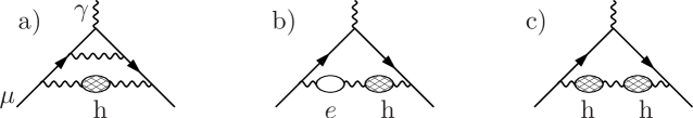
Figure 11: Higher order (HO) vacuum polarization contributions

The relevant kernels for the corresponding dispersion integrals have been calculated analytically in 02BR74 and appropriate series expansions were given in 02Krause96 (for earlier estimates see  02Calmet76 ; 02KNO84 ). Based on my recent compilation of the $e^{+}e^{-}$ data 02FJ06 I obtain

$$a_{\mu}^{\mathrm{had(2)}}=(-100.3\pm 2.2)\>\times 10^{-11}\;,$$ (55)

in accord with previous/other evaluations 02KNO84 ; 02Krause96 ; 02ADH98 ; 02HMNT04 ; 02HMNT06 .

Much more serious problems with non-perturbative hadronic effect we encounter with the hadronic light-by-light (LbL) contribution at $O(\alpha^{3})$ depicted in Fig. 12.

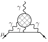
Figure 12: Hadronic light-by-light scattering in $g-2$

Experimentally, we know that $\gamma\gamma\to\mathrm{hadrons}\to\gamma\gamma$ is dominated by the hadrons $\pi^{0},~{}\eta,~{}\eta^{\prime},\cdots$, i.e., single pseudoscalar meson spikes 02LBLfacts , and that $\pi^{0}\to\gamma\gamma$ etc. is governed by the parity odd Wess-Zumino-Witten (WZW) effective Lagrangian

$${\cal L}^{(4)}=-\frac{\alpha N_{c}}{12\ \pi f_{0}}\varepsilon_{\mu\nu\rho\sigma}F^{\mu\nu}A^{\rho}\partial^{\sigma}\pi^{0}+\cdots$$ (56)

which reproduces the Adler-Bell-Jackiw triangle anomaly and which helps in estimating the leading hadronic LbL contribution. $f_{0}$ denotes the pion decay constant $f_{\pi}$ in the chiral limit of massless light quarks. Again, in a low energy effective description, the quasi Goldstone bosons, the pions and kaons play an important role, and the relevant diagrams are displayed in Fig 13.

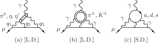
Figure 13: Leading hadronic light–by–light scattering diagrams: the two leading CHPT diagrams (L.D.) and the QPM diagram (S.D.). The charged pion loop is sub-leading only, actually. Diagrams with permuted $\gamma$’s on the $\mu$-line have to be included. $\gamma$-hadron/quark vertices at $q^{2}\neq 0$ are dressed (VMD)

However, as we know from the hadronic VP discussion, the $\rho$ meson is expected to play an important role in the game. It looks natural to apply a vector-meson dominance (VMD) like model. Electromagnetic interactions of pions treated as point-particles would be descried by scalar QED in a first step. However, due to hadronic interactions the photon mixes with hadronic vector-mesons like the $\rho^{0}$. The naive VMD model attempts to take into account this hadronic dressing by replacing the photon propagator as

$$\frac{{\rm i}\>g^{\mu\nu}}{q^{2}}+\cdots\to\frac{{\rm i}\>g^{\mu\nu}}{q^{2}}+\cdots-\frac{{\rm i}\>(g^{\mu\nu}-\frac{q^{\mu}q^{\nu}}{m_{\rho}^{2}})}{q^{2}-m_{\rho}^{2}}=\frac{{\rm i}\>g^{\mu\nu}}{q^{2}}\>\frac{m_{\rho}^{2}}{q^{2}-m_{\rho}^{2}}+\cdots\,,$$

where the ellipses stand for the gauge terms. The main effect is that it provides a damping at high energies with the $\rho$ mass as an effective cut-off (physical version of a Pauli-Villars cut-off). However, the naive VMD model is not compatible with chiral symmetry. The way out is the Resonance Lagrangian Approach (RLA) 02EGPdeR89 , an extended version of CHPT which incorporates vector-mesons in accordance with the basic symmetries. The Hidden Local Symmetry (HLS) 02HLS88 model and the Extended Nambu-Jona-Lasinio (ENJL)  02ENJL96 model are alternative versions of RLA, which are basically equivalent 02Prades99 , for what concerns this application.

Based on such effective field theory (EFT) models, two major efforts in evaluating the full $a_{\mu}^{\mathrm{LbL}}$ contribution were made by Hayakawa, Kinoshita and Sanda (HKS 1995) 02HKS95 , Bijnens, Pallante and Prades (BPP 1995) 02BijnensLBL and Hayakawa and Kinoshita (HK 1998) 02HK98 (see also Kinoshita, Nizic and Okamoto (KNO 1985) 02KNO84 ). Although the details of the calculations are quite different, which results in a different splitting of various contributions, the results are in good agreement and essentially given by the $\pi^{0}$-pole contribution, which was taken with the wrong sign, however. In order to eliminate the cut-off dependence in separating L.D. and S.D. physics, more recently it became favorable to use quark–hadron duality, as it holds in the large $N_{c}$ limit of QCD, for modeling of the hadronic amplitudes 02deRafaelEJLN94 . The infinite series of narrow vector states known to show up in the large $N_{c}$ limit is then approximated by a suitable lowest meson dominance (LMD+V) ansatz 02LMD98 , assumed to be saturated by known low lying physical states of appropriate quantum numbers. This approach was adopted in a reanalysis by Knecht and Nyffeler (KN 2001) 02KnechtNyffeler01 ; 02KNPdeR01 ; 02BCM02 ; 02RMW02 in 2001, in which they discovered a sign mistake in the dominant $\pi^{0},\eta,\eta^{\prime}$ exchange contribution, which changed the central value by $+167\times 10^{-11}$, a 2.8 $\sigma$ shift, and which reduces a larger discrepancy between theory and experiment. More recently Melnikov and Vainshtein (MV 2004) 02MV03 found additional problems in previous calculations, this time in the short distance constraints (QCD/OPE) used in matching the high energy behavior of the effective models used for the $\pi^{0},\eta,\eta^{\prime}$ exchange contribution.

The most important pion-pole term is of the form ($p$ is the muon momentum, $q_{i}$ ($i=1,2,3$) are the virtual photon momenta, two of which are chosen as loop integration variables) 02KnechtNyffeler01

$$a_{\mu}^{\mbox{\tiny{LbL;$\pi^{0}$}}} = -e^{6}\int\frac{\mathrm{d}^{4}q_{1}}{(2\pi)^{4}}\frac{\mathrm{d}^{4}q_{2}}{(2\pi)^{4}}\,\frac{1}{q_{1}^{2}q_{2}^{2}(q_{1}+q_{2})^{2}[(p+q_{1})^{2}-m^{2}][(p-q_{2})^{2}-m^{2}]}$$ (57)

$$\quad\quad\times\left[\frac{{\cal F}_{\pi^{*}\gamma^{*}\gamma^{*}}(q_{2}^{2},q_{1}^{2},q_{3}^{2})\ {\cal F}_{\pi^{*}\gamma^{*}\gamma}(q_{2}^{2},q_{2}^{2},0)}{q_{2}^{2}-m_{\pi}^{2}+{\rm i}\varepsilon}\ T_{1}(q_{1},q_{2};p)\right.$$

$$\quad\quad\quad+\left.\frac{{\cal F}_{\pi^{*}\gamma^{*}\gamma^{*}}(q_{3}^{2},q_{1}^{2},q_{2}^{2})\ {\cal F}_{\pi^{*}\gamma^{*}\gamma}(q_{3}^{2},q_{3}^{2},0)}{q_{3}^{2}-m_{\pi}^{2}+{\rm i}\varepsilon}\ T_{2}(q_{1},q_{2};p)\right]\,,$$

where $T_{1}(q_{1},q_{2};p)$ and $T_{2}(q_{1},q_{2};p)$ are known scalar kinematics factors and ${\cal F}_{\pi^{*}\gamma^{*}\gamma^{*}}(q_{1}^{2},q_{2}^{2},q_{3}^{2})$ is the non-perturbative $\pi^{0}\gamma\gamma$ form factor (FF) whose off-shell form is essentially unknown in the integration range of (57).

A new quality of the problem encountered here is the fact that the integrand depends on 3 invariants $q_{1}^{2}$, $q_{2}^{2}$, $q_{3}^{2}$ $q_{3}=-(q_{1}+q_{2})$. While hadronic VP correlators or the VVA triangle with an external zero momentum vertex only depends on a single invariant $q^{2}$. In the latter case the invariant amplitudes (form factors) may be separated into a low energy part $q^{2}\leq\Lambda^{2}$ (soft) where the low energy effective description applies and a high energy part $q^{2}>\Lambda^{2}$ (hard) where pQCD works. In multi-scale problems, however, there are mixed soft-hard regions where no answer is available in general, unless we have data to constrain the amplitudes in such regions. In our case, only the soft region $q_{1}^{2},q_{2}^{2},q_{3}^{2}\leq\Lambda^{2}$ and the hard region $q_{1}^{2},q_{2}^{2},q_{3}^{2}>\Lambda^{2}$ are under control of either the low energy EFT and of pQCD, respectively. In the mixed soft-hard domains operator product expansions and/or soft versus hard factorization “theorems” à la Brodsky-Farrar 02BrodskyFarrar73 may help. Actually, one more approximation is usually made: the pion-pole approximation ,i.e., the pion-momentum square (first argument of ${\cal F}$) is set equal to $m_{\pi}^{2}$, as the main contribution is expected to come from the pole. Knecht and Nyffeler modeled ${\cal F}_{\pi\gamma^{*}\gamma^{*}}(m_{\pi}^{2},q_{1}^{2},q_{2}^{2})$ in the spirit of the large $N_{c}$ expansion as a “LMD+V” form factor:

$$\scriptsize{\cal F}_{\pi\gamma^{*}\gamma^{*}}(m_{\pi}^{2},q_{1}^{2},q_{2}^{2})=\frac{f_{\pi}}{3}~{}\frac{q_{1}^{2}q_{2}^{2}(q_{1}^{2}+q_{2}^{2})+h_{1}(q_{1}^{2}+q_{2}^{2})^{2}+h_{2}q_{1}^{2}q_{2}^{2}+h_{5}(q_{1}^{2}+q_{2}^{2})+h_{7}}{(q_{1}^{2}-M_{1}^{2})(q_{1}^{2}-M_{2}^{2})(q_{2}^{2}-M_{1}^{2})(q_{2}^{2}-M_{2}^{2})}\,,$$ (58)

with $h_{7}=-(N_{c}M_{1}^{4}M_{2}^{4}/4\pi^{2}f_{\pi}^{2})$, $f_{\pi}\simeq 92.4~{}\mathrm{MeV}$. An important constraint comes from the pion-pole form factor ${\cal F}_{\pi\gamma^{*}\gamma}(m_{\pi}^{2},-Q^{2},0)$, which has been measured by CELLO 02CELLO90 and CLEO 02CLEO98 . Experiments are in fair agreement with the Brodsky–Lepage 02LepageBrodsky80 form

$${\cal F}_{\pi\gamma^{*}\gamma}(m_{\pi}^{2},-Q^{2},0)\simeq-\frac{N_{c}}{12\pi^{2}f_{\pi}}\frac{1}{1+(Q^{2}/8\pi^{2}f_{\pi}^{2})}$$ (59)

which interpolates between a $1/Q^{2}$ asymptotic behavior and the constraint from $\pi^{0}$ decay at $Q^{2}=0$. This behavior requires $h_{1}=0$. Identifying the resonances with $M_{1}=M_{\rho}=769~{}{\rm MeV}$, $M_{2}=M_{\rho^{\prime}}=1465~{}{\rm MeV}$, the phenomenological constraint fixes $h_{5}=6.93~{}{\rm GeV}^{4}$. $h_{2}$ will be fixed by later. As the previous analyses, Knecht and Nyffeler apply the above VMD type form factor on both ends of the pion line. In fact at the vertex attached to the external zero momentum photon, this type of pion-pole form factor cannot apply for kinematical reasons: when $q^{\mu}_{\mathrm{ext}}=0$ not ${\cal F}_{\pi\gamma^{*}\gamma}(m_{\pi}^{2},-Q^{2},0)$ but ${\cal F}_{\pi^{*}\gamma^{*}\gamma}(q_{2}^{2},q_{2}^{2},0)$ is the relevant object to be used, where $q_{2}$ is to be integrated over. However, for large $q_{2}^{2}$ the pion must be far off-shell, in which case the pion exchange effective representation becomes obsolete. Melnikov and Vainshtein reanalyzed the problem by performing an operator product expansion (OPE) for $q_{1}^{2}\simeq q_{2}^{2}\gg(q_{1}+q_{2})^{2}\sim m_{\pi}^{2}$. In the chiral limit this analysis reveals that the external vertex is determined by the exactly known ABJ anomaly ${\cal F}_{\pi\gamma\gamma}(m_{\pi}^{2},0,0)=-1/(4\pi^{2}f_{\pi})$. This means that in the chiral limit there is no VMD like damping at high energies at the external vertex. However, the absence of a damping in the chiral limit does not prove that there is no damping in the real world with non-vanishing quark masses. In fact, the quark triangle-loop in this case provides a representation of the $\pi^{0*}\gamma^{*}\gamma^{*}$ amplitude given by

$$F^{\mathrm{CQM}}_{\pi^{0*}\gamma^{*}\gamma^{*}}(q^{2},p_{1}^{2},p_{2}^{2}) \equiv (-4\pi^{2}f_{\pi})\>{\cal F}_{\pi^{*}\gamma^{*}\gamma^{*}}(q^{2},p_{1}^{2},p_{2}^{2})=2m_{q}^{2}\>C_{0}(m_{q};q^{2},p_{1}^{2},p_{2}^{2})$$ (60)

$$\equiv \int[\mathrm{d}\alpha]\>\frac{2m_{q}^{2}}{m_{q}^{2}-\alpha_{2}\alpha_{3}p_{1}^{2}-\alpha_{3}\alpha_{1}p_{2}^{2}-\alpha_{1}\alpha_{2}q^{2}}\;,$$

where $[\mathrm{d}\alpha]=\mathrm{d}\alpha_{1}\mathrm{d}\alpha_{2}\mathrm{d}\alpha_{3}\>\delta(1-\alpha_{1}-\alpha_{2}-\alpha_{3})$ and $m_{q}$ is a constituent quark mass ($q=u,d,s$). For $p_{1}^{2}=p_{2}^{2}=q^{2}=0$ we obtain $F^{\mathrm{CQM}}_{\pi^{0*}\gamma^{*}\gamma^{*}}(0,0,0)=1$, which is the proper ABJ anomaly. Note the symmetry of $C_{0}$ under permutations of the arguments ($p_{1}^{2},p_{2}^{2},q^{2}$). For large $p_{1}^{2}$ at $p_{2}^{2}\sim 0,~{}q^{2}\sim 0$ or $p_{1}^{2}\sim p_{2}^{2}$ at $q^{2}\sim 0$ the asymptotic behavior is given by

$$F^{\mathrm{CQM}}_{\pi^{0}\gamma^{*}\gamma}(0,p_{1}^{2},0)\sim r\>\ln^{2}r\;,\;\;F^{\mathrm{CQM}}_{\pi^{0}\gamma^{*}\gamma^{*}}(0,p_{1}^{2},p_{1}^{2})\sim 2\>r\>\ln r$$ (61)

where $r=\frac{m_{q}^{2}}{-p_{1}^{2}}$. The same behavior follows for $q^{2}\sim p_{1}^{2}$ at $p_{2}^{2}\sim 0$. Note that in all cases we have the same power behavior $\sim m_{q}^{2}/p_{i}^{2}$ modulo logarithms. Thus at high energies the anomaly gets screened by chiral symmetry breaking effects.

We therefore advocate to use consistently dressed form factors as inferred from the resonance Lagrangian approach. However, other effects which were first considered in 02MV03 must be taken into account:
1) the constraint on the twist four $(1/q^{4})$-term in the OPE requires $h_{2}=-10$ GeV² in the Knecht-Nyffeler from factor (58): $\delta a_{\mu}\simeq+5\pm 0$
2) the contributions from the $f_{1}$ and $f_{1}^{\prime}$ isoscalar axial-vector mesons: $\delta a_{\mu}\simeq+10\pm 4$ (using dressed photons)
3) for the remaining effects: scalars ($f_{0}$) $+$ dressed $\pi^{\pm},K^{\pm}$ loops $+$ dressed quark loops: $\delta a_{\mu}\simeq+2\pm 6$
Note that the remaining terms have been evaluated in 02HKS95 ; 02BijnensLBL only. The splitting into the different terms is model dependent and only the sum should be considered: the results read $-5\pm 13$ (BPP) and $5.2\pm 13.7$ (HKS) and hence the true contribution remains unclear.

An overview of results is presented in Table 3. The last column gives my estimates base on 02HKS95 ; 02BijnensLBL ; 02KnechtNyffeler01 ; 02MV03 . The “no FF” column shows results for undressed photons (no form factor).

Table 3: LbL: Summary of most recent results for $a_{\mu}\times 10^{11}$

	no FF	BPP	HKS	KN	MV	FJ
$\pi^{0},\eta,\eta^{\prime}$	$+\infty~{}~{}$	$85\pm 13~{}$	$82.7\pm 6.4$	$83\pm 12$	$114\pm 10$	$88\pm 12$
axial vector		$2.5\pm 1.0$	$1.7\pm 0.0$		$22\pm~{}5$	$10\pm~{}4$
scalar		$-6.8\pm 2.0$	$-$	$-$	$-$	$0\pm~{}7$
$\pi,K$ loops	$-49.8~{}$	$-19\pm 13~{}$	$-4.5\pm 8.1$		$0\pm 10$	$-19\pm 13$
quark loops	$~{}~{}62(3)~{}$	$21\pm~{}3~{}$	$9.7\pm 11.1$	$-$	$-$	$21\pm~{}3$
total		$83\pm 32~{}$	$89.6\pm 15.4$	$80\pm 40$	$136\pm 25$	$100\pm 39$

The constant WZW form factor yields a divergent result, applying a cut-off $\Lambda$ one obtains 02KNPdeR01 $(\alpha/\pi)^{3}{\cal C}\ln^{2}\Lambda$, with an universal coefficient ${\cal C}=N_{c}^{2}m_{\mu}^{2}/(48\pi^{2}f_{\pi}^{2})$; in the VMD dressed cases $M_{V}$ represents the cut-off $\Lambda\to M_{V}$ if $M_{V}\to\infty$.

5 Theory Confronting the Experiment

The following Tab. 4 collects the typical contributions to $a_{\mu}$ evaluated in terms of $\alpha$ determined via $a_{e}$ (14).

Table 4: The various types of contributions to $a_{\mu}$ in units $10^{-6}$, ordered according to their size (L.O. lowest order, H.O. higher order, LbL. light–by–light)

L.O. universal	$~{}~{}1161$.	$409\,73~{}~{}~{}(0)$
$e$–loops	$6$.	$194\,57~{}~{}~{}(0)$
H.O. universal	$-1$.	$757\,55~{}~{}~{}(0)$
L.O. hadronic	$0$.	$069\,21~{}~{}(56)$
L.O. weak	$0$.	$001\,95~{}~{}~{}(0)$
H.O. hadronic	$-0$.	$001\,00~{}~{}~{}(2)$
LbL. hadronic	$0$.	$001\,00~{}~{}(39)$
$\tau$–loops	$0$.	$000\,43~{}~{}~{}(0)$
H.O. weak	$-0$.	$000\,41~{}~{}~{}(2)$
$e$+$\tau$–loops	$0$.	$000\,01~{}~{}~{}(0)$
theory	$1165$.	$917\,93~{}~{}(68)$
experiment	$1165$.	$920\,80~{}~{}(63)$

The world average experimental muon magnetic anomaly, dominated by the very precise BNL result, now is 02BNL04

$$a_{\mu}^{\mathrm{exp}}=1.16592080(63)\times 10^{-3}$$ (62)

(relative uncertainty $5.4\times 10^{-7}$), which confronts the SM prediction

$$a_{\mu}^{\mathrm{the}}=1.16591793(68)\times 10^{-3}\;.$$ (63)

Fig. 14 illustrates the improvement achieved by the BNL experiment. The theoretical predictions mainly differ by the L.O. hadronic effects, which also dominate the theoretical error. A deviation between theory and experiment of about 3 $\sigma$ was persisting since the first precise BNL result was released in 2000, in spite of progress in theory and experiment since.

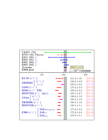
Figure 14: Comparison between theory and experiment. Results differ by different L.O. hadronic vacuum polarizations and variants of the LbL contribution. Some estimates include isospin rotated $\tau$–data ($+\tau$)). The last entry FJ06 also illustrates the effect of using different LbL estimations: 1) Bijnens, Pallante, Prades (BPP) 02BijnensLBL , Hayakawa, Kinoshita (HK) 02HK98 and Knecht, Nyffeler (KN) 02KnechtNyffeler01 ; 2) my estimation based on the other evaluations; 3) the Melnikov, Vainshtein (MV) 02MV03 estimate of the LbL contribution. EJ95 vs. FJ06 illustrates the improvement of the $e^{+}e^{-}$-data between 1995 and now (see also Tab. 2). E969 is a possible follow-up experiment of E821 proposed recently 02LeeRob03

Note that the experimental uncertainty is still statistics dominated. Thus just running the BNL experiment longer could have substantially improved the result. Originally the E821 goal was $\delta a_{\mu}^{\mathrm{exp}}\sim 40\times 10^{-11}$. Fig. 15 illustrates the sensitivity to various contributions and how it developed in time. The dramatic

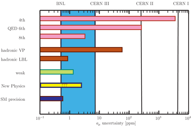
Figure 15: Sensitivity of g-2 experiments to various contributions. The increase in precision with the BNL $g-2$ experiment is shown as a gray vertical band. New Physics is illustrated by the deviation $(a_{\mu}^{\mathrm{exp}}-a_{\mu}^{\mathrm{the}})/a_{\mu}^{\mathrm{exp}}$

$(m_{\mu}/m_{e})^{2}$ enhancement in the sensitivity of $a_{\mu}$, relative to $a_{e}$, to physics at scales $M$ larger than $m_{\mu}$, which is scaling like $(m_{\mu}/M)^{2}$, and the more than one order of magnitude improvement of the experimental accuracy has brought many SM effects into the focus of the interest. Not only are we testing now the 4–loop QED contribution, higher order hadronic VP effects, the infamous hadronic LbL contribution and the weak loops, we are reaching or limiting possible New Physics at a level of sensitivity which causes a lot of excitement. “New Physics” is displayed in the figure as the ppm deviation of

$$\delta a_{\mu}=a_{\mu}^{\mathrm{exp}}-a_{\mu}^{\mathrm{the}}=(287\pm 91)\times 10^{-11}$$ (64)

which is $3.2\>\sigma$. We note that the theory error is somewhat larger than the experimental one. It is fully dominated by the uncertainty of the hadronic low energy cross–section data, which determine the hadronic vacuum polarization and, partially, by the uncertainty of the hadronic light–by–light scattering contribution.

As we notice, the enhanced sensitivity to “heavy” physics is somehow good news and bad news at the same time: the sensitivity to “New Physics” we are always hunting for at the end is enhanced due to

$$a^{\mathrm{NP}}_{\ell}\sim\left(\frac{m_{\ell}}{M_{\rm NP}}\right)^{2}$$

by the mentioned mass ratio square, but at the same time also scale dependent SM effects are dramatically enhanced, and the hadronic ones are not easy to estimate with the desired precision.

6 Prospects

The BNL muon $g-2$ experiment has determined $a_{\mu}$ as given by (62), reaching the impressive precision of 0.54 ppm, a 14–fold improvement over the CERN experiment from 1976. Herewith, a new quality has been achieved in testing the SM and in limiting physics beyond it. The main achievements and problems are

• a substantial improvement in testing CPT for muons,

• a first confirmation of the fairly small weak contribution at the $2-3~{}\sigma$ level,

• the hadronic vacuum polarization contribution, obtained via experimental $e^{+}e^{-}$ annihilation data, limits the theoretical precision at the $1~{}\sigma$ level,

• now and for the future the hadronic light-by-light scattering contribution, which amounts to about $2\sigma$, is not far from being as important as the weak contribution; present calculations are model-dependent, and may become the limiting factor for future progress.

At present a $3.2\sigma$ deviation between theory and experiment is observed and the “missing piece” (64) could hint to new physics, but at the same time rules out big effects predicted by many possible extensions of the SM.

Usually, new physics (NP) contributions are expected to produce contributions proportional to $m_{\mu}^{2}/M_{\mathrm{NP}}^{2}$ and thus are expected to be suppressed by $M_{W}^{2}/M_{\mathrm{NP}}^{2}$ relative to the weak contribution.

The most promising theoretical scenarios are supersymmetric (SUSY) extensions of the SM, in particular the minimal one (MSSM). Each SM state $X$ has an associated supersymmetric “sstate” $\tilde{X}$ where sfermions are bosons and sbosons are fermions. This implements the fermion $\leftrightarrow$ boson supersymmetry. In addition, an anomaly free MSSM requires a second complex Higgs doublet, which means 4 additional scalars and their SUSY partners. Both Higgs fields exhibit a neutral scalar which aquire vacuum expectation values $v_{1}$ and $v_{2}$. Typical supersymmetric contributions to $a_{\mu}$ stem from smuon–neutralino and sneutrino-chargino loops Fig. 16.

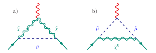
Figure 16: Physics beyond the SM: leading SUSY contributions to $g-2$ in supersymmetric extension of the SM

Some contributions are enhanced by $\tan\beta\equiv\frac{v_{2}}{v_{1}}$ which may be large (in some cases of order $m_{t}/m_{b}\approx 40$). One obtains 02Moroi95 (for the extension to 2-loops see 02HSW03 )

(65)

$\widetilde{m}=m_{\rm SUSY}$ a typical SUSY loop mass and $\mu$ is the Higgsino mass term. In the large $\tan\beta$ regime we have

$$\left|a_{\mu}^{\rm SUSY}\right|\simeq 123\times 10^{-11}\left(\frac{100{\rm\ GeV}}{\widetilde{m}}\right)^{2}\tan\beta\;.$$ (66)

$a_{\mu}^{\rm SUSY}$ generally has the same sign as the $\mu$-parameter. The deviation (64) requires positive $\mathrm{sign}(\mu)$ and if identified as a SUSY contribution

$$\widetilde{m}\simeq(65.5\mbox{ GeV})\sqrt{\tan\beta}\;.$$ (67)

Negative $\mu$ models give the opposite sign contribution to $a_{\mu}$ and are strongly disfavored. For $\tan\beta$ in the range $2\div 40$ one obtains

$$\widetilde{m}\simeq 92-414\mbox{ GeV}\;,$$ (68)

precisely the range where SUSY particles are often expected. For a variety of non-SUSY extensions of the SM typically $\left|a_{\mu}(\mbox{NP})\right|\simeq{\cal C}\>m_{\mu}^{2}/M^{2}$ where ${\cal C}=O(1)$ [or $O(\alpha/\pi)$ if radiatively induced]. The current constraint suggests (very roughly) $M\simeq 1.7-2.4\mbox{ TeV}$ [$M\simeq 87-121\mbox{ GeV}$]. The ${\cal C}=O(1)$ assumption is problematic, however, since no tree level contribution can be tolerated. For a more elaborate discussion and further references I refer to 02CzMa01 . Note that the most natural leading contributions in extensions of the SM are 1-loop contributions similar to the leading weak effects or the leading MSSM contributions. However, mass limits set by LEP and Tevatron make it highly non-trivial to reconcile the observed deviation to many of the new physics scenarios. Only the $\tan\beta$ enhanced contributions in SUSY extensions of the SM for $\mu>0$ and large enough $\tan\beta$ may explain the “missing contribution”. Two Higgs doublet models 02Krawczyk05 have similar possibilities. Physics beyond the SM of course not only contributes to $a_{\mu}$ but also to other observables like to the branching fraction $Br(b\to s\gamma)=(3.40\pm 0.28)\times 10^{-4}$ or to the $W$ mass prediction $M_{W}=80.392(29)~{}\mathrm{GeV}$. In the $R$–parity conserving MSSM the lightest neutralino is stable and therefore is a candidate for cold dark matter in the universe. From the precision mapping of the anisotropies in the cosmic microwave background, the WMAP collaboration has determined the relict density of cold dark matter to $\Omega{\rm h}^{2}=0.1126\pm 0.0081$. This sets severe constraints on the SUSY parameter space (see for example 02HBaeretal04 ).

Of course, for a specific model, one must check that the sign of the induced $a_{\mu}^{\rm NP}$is in accord with experiment (i.e. it should be positive).

Plans for a new $g-2$ experiment exist 02LeeRob03 . In fact, the impressive 0.54 ppm precision measurement by the E821collaboration at Brookhaven was still limited by statistical errors rather than by systematic ones. Therefore an upgrade of the experiment at Brookhaven or J-PARC (Japan) is supposed to be able to reach a precision of 0.2 ppm (Brookhaven) or 0.1 ppm (J-PARC).

For the theory this poses a new challenge. It is clear that on the theory side, a reduction of the leading hadronic uncertainty is required, which actually represents a big experimental challenge: one has to attempt cross-section measurements at the 1% level up to $J/\psi$[$\Upsilon$] energies (5[10] GeV). Such measurements would be crucial for the muon $g-2$ as well as for a more precise determination of the running fine structure constant $\alpha_{\rm QED}(E)$. In particular, $e^{+}e^{-}$ low energy cross section measurements in the region between 1 and 2.5 GeV 02VEPP2000 ; 02KLOE2 are able to substantially improve the accuracy of $a_{\mu}^{\mathrm{had(1)}}$ and $\alpha_{\rm QED}(M_{Z})$ 02FJ06 .

New ideas are required to get less model–dependent estimations of the hadronic LbL contribution. Here, new high statistics experiments attempting to measure the $\pi^{0}\gamma^{*}\gamma^{*}$ form factor ${\cal F}(m_{\pi}^{2},-Q_{1}^{2},-Q_{2}^{2})$ for $Q_{1}^{2}\sim Q_{2}^{2}$ and a scan of the light-by-light off-shell amplitude via $e^{+}e^{-}\to e^{+}e^{-}\gamma^{*}\gamma^{*}\to e^{+}e^{-}\gamma\gamma$ would be of great help. Certainly lattice QCD studies 02BluAub06 will be able to shed light on these non-perturbative problems in future.

In any case the muon $g-2$ story is a beautiful example which illustrates the experience that the closer we look the more there is to see, but also the more difficult it gets to predict and interprete what we see. Even facing problems to pin down precisely the hadronic effects, the achievements in the muon $g-2$ is a big triumph of science. Here all kinds of physics meet in one single number which is the result of a truly ingenious experiment. Only getting all details in all aspects correct makes this number a key quantity for testing our present theoretical framework in full depth. It is the result of tremendous efforts in theory and experiment and on the theory side has contributed a lot to push the development of new methods and tools such as computer algebra as well as high precision numerical methods which are indispensable to handle the complexity of hundreds to thousands of high dimensional integrals over singular integrands suffering from huge cancellations of huge numbers of terms. Astonishing that all this really works!

Note added: After completion of this work a longer review article appeared MdeRLR07 , which especially reviews the experimental aspects in much more depth than the present essay. For a recent reanalysis of the light-by-light contribution we refer the reader to BijnensPrades07 , which presents the new estimate $a_{\mu}^{\rm LbL}=(110\pm 40)\times 10^{-11}$.

Acknowledgments

This extended update and overview was initiated by a talk given at the International Workshop on Precision Physics of Simple Atomic Systems (PSAS 2006). It is a pleasure to thank the organizers and in particular to Savely Karshenboim for the kind invitation to this stimulating meeting. The main new results were first presented at the Kazimirez Final EURIDICE Meeting. Thanks to Maria Krawczyk and Henryk H. Czyż for the kind hospitality in Kazimirez. Particular thanks to Andreas Nyffeler and to Simon Eidelman for many enlightening discussions. Thanks also to Oleg Tarasov and Rainer Sommer for helpful discussions and for carefully reading the manuscript. Many thanks to B. Lee Roberts and the members of the E821 collaboration for many stimulating discussions over the years and for providing me some of the figures. Special thanks go to Wolfgang Kluge, Klaus Mönig, Stefan Müller, Federico Nguyen, Giulia Pancheri and Graziano Venanzoni for numerous stimulating discussions and their continuous interest. I gratefully acknowledge the kind hospitality extended to me by Frascati National Laboratory and the KLOE group. This work was supported in part by EC-Contracts HPRN-CT-2002-00311 (EURIDICE) and RII3-CT-2004-506078 (TARI).

References

- (1) P. A. M. Dirac, Proc. Roy. Soc. A 117 (1928) 610; A 118 (1928) 351
- (2) P. Kusch, H. M. Foley, Phys. Rev. 73 (1948) 421; Phys. Rev. 74 (1948) 250
- (3) J. S. Schwinger, Phys. Rev. 73 (1948) 416
- (4) R. L. Garwin, L. Lederman, M. Weinrich, Phys. Rev. 105 (1957) 1415
- (5) J. I. Friedman, V .L. Telegdi, Phys. Rev. 105 (1957) 1681
- (6) R. L. Garwin et al., Phys. Rev. 118 (1960) 271
- (7) G. Charpak et al., Phys. Lett. 1 (1962) 16
- (8) J. Bailey et al., Nuovo Cimento A 9 (1972) 369
- (9) J. Aldins et al., Phys. Rev. Lett. 23 (1969) 441; Phys. Rev. D 1 (1970) 2378
- (10) J. Bailey et al., Nucl. Phys. B 150 (1979) 1
- (11) R. M. Carey et al., Phys. Rev. Lett. 82 (1999) 1632; H. N. Brown et al., Phys. Rev. D 62 (2000) 091101; Phys. Rev. Lett. 86 (2001) 2227; G. W. Bennett et al., Phys. Rev. Lett. 89 (2002) 101804 [Erratum-ibid. 89 (2002) 129903]; Phys. Rev. Lett. 92 (2004) 161802
- (12) G. W. Bennett et al. [Muon g-2 Collaboration], Phys. Rev. D 73 (2006) 072003
- (13) B. Odom, D. Hanneke, B. D’Urso, G. Gabrielse Phys. Rev. Lett. 97 (2006) 030801
- (14) G. Gabrielse, D. Hanneke, T. Kinoshita, M. Nio, B. Odom, Phys. Rev. Lett. 97 (2006) 030802
- (15) T. Aoyama, M. Hayakawa, T. Kinoshita, M. Nio, arXiv:0706.3496 [hep-ph]
- (16) S. Eidelman et al. [Particle Data Group Collaboration], Phys. Lett. B 592 (2004) 1
- (17) P. J. Mohr, B. N. Taylor, Rev. Mod. Phys. 72 (2000) 351; 77 (2005) 1
- (18) A. Petermann, Helv. Phys. Acta 30 (1957) 407; Nucl. Phys. 5 (1958) 677
- (19) C. M. Sommerfield, Phys. Rev. 107 (1957) 328; Ann. Phys. (N.Y.) 5 (1958) 26
- (20) S. Laporta, E. Remiddi, Phys. Lett. B 379 (1996) 283
- (21) J. A. Mignaco, E. Remiddi, Nuovo Cim. A 60 (1969) 519; R. Barbieri, E. Remiddi, Phys. Lett. B 49 (1974) 468; Nucl. Phys. B 90 (1975) 233; R. Barbieri, M. Caffo, E. Remiddi, Phys. Lett. B 57 (1975) 460; M. J. Levine, E. Remiddi, R. Roskies, Phys. Rev. D 20 (1979) 2068; S. Laporta, E. Remiddi, Phys. Lett. B 265 (1991) 182; S. Laporta, Phys. Rev. D 47 (1993) 4793; Phys. Lett. B 343 (1995) 421; S. Laporta, E. Remiddi, Phys. Lett. B 356 (1995) 390
- (22) T. Kinoshita, Phys. Rev. Lett. 75 (1995) 4728
- (23) T. Kinoshita, W. B. Lindquist, Phys. Rev. D 27 (1983) 867; 27 (1983) 877; 27 (1983) 886; 39 (1989) 2407; 42 (1990) 636
- (24) V. W. Hughes, T. Kinoshita, Rev. Mod. Phys. 71 (1999) S133; T. Kinoshita, Quantum Electrodynamics, 1st edn (World Scientific, Singapore 1990) pp 997
- (25) T. Kinoshita, M. Nio, Phys. Rev. D 73 (2006) 013003
- (26) H. Suura, E. Wichmann, Phys. Rev. 105 (1957) 1930; A. Petermann, Phys. Rev. 105 (1957) 1931
- (27) H. H. Elend, Phys. Lett. 20 (1966) 682; Erratum-ibid. 21 (1966) 720
- (28) B. E. Lautrup, E. De Rafael, Nuovo Cim. A 64 (1969) 322
- (29) B. Lautrup, Phys. Lett. B 69 (1977) 109
- (30) B. E. Lautrup, E. de Rafael, Nucl. Phys. B 70 (1974) 317
- (31) G. Li, R. Mendel, M. A. Samuel, Phys. Rev. D 47 (1993) 1723
- (32) T. Kinoshita, Nuovo Cim. B 51 (1967) 140
- (33) B. E. Lautrup, E. De Rafael, Phys. Rev. 174 (1968) 1835; B. E. Lautrup, M. A. Samuel, Phys. Lett. B 72 (1977) 114
- (34) M. A. Samuel, G. Li, Phys. Rev. D 44 (1991) 3935 [Errata-ibid. D 46 (1992) 4782; D 48 (1993) 1879]
- (35) S. Laporta, Nuovo Cim. A 106 (1993) 675
- (36) S. Laporta, E. Remiddi, Phys. Lett. B 301 (1993) 440
- (37) J. H. Kühn, A. I. Onishchenko, A. A. Pivovarov, O. L. Veretin, Phys. Rev. D 68 (2003) 033018
- (38) R. S. Van Dyck, P. B. Schwinberg, H. G. Dehmelt, Phys. Rev. Lett. 59 (1987) 26
- (39) P. J. Mohr, B. N. Taylor, Rev. Mod. Phys. 77 (2005) 1
- (40) P. Cladé et al., Phys. Rev. Lett. 96 (2006) 033001
- (41) V. Gerginov et al., Phys. Rev. A 73 (2006) 032504
- (42) A. Czarnecki, M. Skrzypek, Phys. Lett. B 449 (1999) 354
- (43) S. Friot, D. Greynat, E. De Rafael, Phys. Lett. B 628 (2005) 73
- (44) M. Passera, J. Phys. G 31 (2005) R75; Phys. Rev. D 75 (2007) 013002; Nucl. Phys. Proc. Suppl. 162 (2006) 242; hep-ph/0702027
- (45) M. Caffo, S. Turrini, E. Remiddi, Phys. Rev. D 30 (1984) 483; E. Remiddi, S. P. Sorella, Lett. Nuovo Cim. 44 (1985) 231; D. J. Broadhurst, A. L. Kataev, O. V. Tarasov, Phys. Lett. B 298 (1993) 445; S. Laporta, Phys. Lett. B 312 (1993) 495; P. A. Baikov, D. J. Broadhurst, hep-ph/9504398
- (46) T. Kinoshita, M. Nio, Phys. Rev. Lett. 90 (2003) 021803; Phys. Rev. D 70 (2004) 113001
- (47) S. G. Karshenboim, Phys. Atom. Nucl. 56 (1993) 857 [Yad. Fiz. 56N6 (1993) 252]
- (48) T. Kinoshita, M. Nio, Phys. Rev. D 73 (2006) 053007
- (49) A. L. Kataev, Nucl. Phys. Proc. Suppl. 155 (2006) 369; hep-ph/0602098; Phys. Rev. D 74 (2006) 073011
- (50) W. A. Bardeen, R. Gastmans, B. Lautrup, Nucl. Phys. B 46 (1972) 319; G. Altarelli, N. Cabibbo, L. Maiani, Phys. Lett. B 40 (1972) 415; R. Jackiw, S. Weinberg, Phys. Rev. D 5 (1972) 2396; I. Bars, M. Yoshimura, Phys. Rev. D 6 (1972) 374; K. Fujikawa, B. W. Lee, A. I. Sanda, Phys. Rev. D 6 (1972) 2923
- (51) E. A. Kuraev, T. V. Kukhto, A. Schiller, Sov. J. Nucl. Phys. 51 (1990) 1031 [Yad. Fiz. 51 (1990) 1631]; T. V. Kukhto, E. A. Kuraev, A. Schiller, Z. K. Silagadze, Nucl. Phys. B 371 (1992) 567
- (52) A. Czarnecki, B. Krause, W. Marciano, Phys. Rev. D 52 (1995) R2619
- (53) S. Peris, M. Perrottet, E. de Rafael, Phys. Lett. B 355 (1995) 523
- (54) M. Knecht, S. Peris, M. Perrottet, E. de Rafael, JHEP 0211 (2002) 003
- (55) G. Degrassi, G. F. Giudice, Phys. Rev. 58D (1998) 053007
- (56) A. Czarnecki, W. J. Marciano, A. Vainshtein, Phys. Rev. D 67 (2003) 073006
- (57) A. Vainshtein, Phys. Lett. B 569 (2003) 187
- (58) M. Knecht, S. Peris, M. Perrottet, E. de Rafael, JHEP 0403 (2004) 035.
- (59) F. Jegerlehner, O. V. Tarasov, Phys. Lett. B 639 (2006) 299
- (60) E. D’Hoker, Phys. Rev. Lett. 69 (1992) 1316
- (61) A. Czarnecki, B. Krause, W. J. Marciano, Phys. Rev. Lett. 76 (1996) 3267
- (62) S. Heinemeyer, D. Stöckinger, G. Weiglein, Nucl. Phys. B 699 (2004) 103
- (63) T. Gribouk, A. Czarnecki, Phys. Rev. D 72 (2005) 053016
- (64) H. Fritzsch, M. Gell-Mann, H. Leutwyler, Phys. Lett. 47B (1973) 365
- (65) H. D. Politzer, Phys. Rev. Lett. 30 (1973) 1346; D. Gross, F. Wilczek, Phys. Rev. Lett. 30 (1973) 1343
- (66) S. G. Gorishnii, A. L. Kataev, S. A. Larin, Phys. Lett. B 259 (1991) 144; L. R. Surguladze, M. A. Samuel, Phys. Rev. Lett. 66 (1991) 560 [Erratum-ibid. 66 (1991) 2416]; K. G. Chetyrkin, Phys. Lett. B 391 (1997) 402.
- (67) K. G. Chetyrkin, J. H. Kühn, Phys. Lett. B 342 (1995) 356; K. G. Chetyrkin, R. V. Harlander, J. H. Kühn, Nucl. Phys. B 586 (2000) 56 [Erratum-ibid. B 634 (2002) 413].
- (68) R. V. Harlander, M. Steinhauser, Comput. Phys. Commun. 153 (2003) 244.
- (69) S. Eidelman, F. Jegerlehner, Z. Phys. C 67 (1995) 585.
- (70) A. E. Blinov et al. [MD-1 Collaboration], Z. Phys. C 70 (1996) 31
- (71) J. Z. Bai et al. [BES Collaboration], Phys. Rev. Lett. 84 (2000) 594; Phys. Rev. Lett. 88 (2002) 101802
- (72) R. R. Akhmetshin et al. [CMD-2 Collaboration], Phys. Lett. B 578 (2004) 285; Phys. Lett. B 527 (2002) 161
- (73) A. Aloisio et al. [KLOE Collaboration], Phys. Lett. B 606 (2005) 12
- (74) M. N. Achasov et al. [SND Collaboration], J. Exp. Theor. Phys. 103 (2006) 380 [Zh. Eksp. Teor. Fiz. 130 (2006) 437]
- (75) V. M. Aulchenko et al. [CMD-2 Collaboration], JETP Lett. 82 (2005) 743 [Pisma Zh. Eksp. Teor. Fiz. 82 (2005) 841]; R. R. Akhmetshin et al., JETP Lett. 84 (2006) 413 [Pisma Zh. Eksp. Teor. Fiz. 84 (2006) 491]; hep-ex/0610021
- (76) F. Jegerlehner, Nucl. Phys. Proc. Suppl. 162 (2006) 22 [hep-ph/0608329]
- (77) M. Davier, S. Eidelman, A. Höcker, Z. Zhang, Eur. Phys. J. C 27 (2003) 497; ibid. 31 (2003) 503
- (78) F. Jegerlehner, J. Phys. G 29 (2003) 101; S. Ghozzi, F. Jegerlehner, Phys. Lett. B 583 (2004) 222.
- (79) S. Narison, Phys. Lett. B 568 (2003) 231
- (80) V. V. Ezhela, S. B. Lugovsky, O. V. Zenin, hep-ph/0312114.
- (81) K. Hagiwara, A. D. Martin, D. Nomura, T. Teubner, Phys. Lett. B 557 (2003) 69; Phys. Rev. D 69 (2004) 093003
- (82) J. F. de Troconiz, F. J. Yndurain, Phys. Rev. D 71 (2005) 073008
- (83) S. Eidelman, Proceedings of the XXXIII International Conference on High Energy Physics, July 27 – August 2, 2006, Moscow (Russia), World Scientific, to appear; M. Davier, hep-ph/0701163
- (84) K. Hagiwara, A. D. Martin, D. Nomura, T. Teubner, hep-ph/0611102
- (85) H. Leutwyler, hep-ph/0212324; G. Colangelo, Nucl. Phys. Proc. Suppl. 131 (2004) 185
- (86) R. Alemany, M. Davier, A. Höcker, Eur. Phys. J. C 2 (1998) 123.
- (87) R. Barbieri, E. Remiddi, Phys. Lett. B 49 (1974) 468; Nucl. Phys. B 90 (1975) 233
- (88) B. Krause, Phys. Lett. B 390 (1997) 392
- (89) J. Calmet, S. Narison, M. Perrottet, E. de Rafael, Phys. Lett. B 61 (1976) 283
- (90) T. Kinoshita, B. Nizic, Y. Okamoto, Phys. Rev. Lett. 52 (1984) 717; Phys. Rev. D 31 (1985) 2108
- (91) H. Kolanoski, P. Zerwas, Two-Photon Physics, In: High Energy Electron-Positron Physics, ed. A. Ali, P. Söding, (World Scientific, Singapore 1988) pp 695–784; D. Williams et al. [Crystal Ball Collaboration], SLAC-PUB-4580, 1988, unpublished
- (92) G. Ecker, J. Gasser, A. Pich, E. de Rafael, Nucl. Phys. B 321 (1989) 311; G. Ecker, J. Gasser, H. Leutwyler, A. Pich, E. de Rafael, Phys. Lett. B 223 (1989) 425
- (93) M. Bando, T. Kugo, S. Uehara, K. Yamawaki, T. Yanagida, Phys. Rev. Lett. 54 (1985) 1215; M. Harada, K. Yamawaki, Phys. Rept. 381 (2003) 1
- (94) A. Dhar, R. Shankar, S. R. Wadia, Phys. Rev. D 31 (1985) 3256; D. Ebert, H. Reinhardt, Phys. Lett. B 173 (1986) 453; J. Bijnens, Phys. Rept. 265 (1996) 369
- (95) J. Prades, Z. Phys. C63, 491 (1994); Erratum: Eur. Phys. J. C11, 571 (1999).
- (96) M. Hayakawa, T. Kinoshita, A. I. Sanda, Phys. Rev. Lett. 75 (1995) 790; Phys. Rev. D 54 (1996) 3137
- (97) J. Bijnens, E. Pallante, J. Prades, Phys. Rev. Lett. 75 (1995) 1447 [Erratum-ibid. 75 (1995) 3781]; Nucl. Phys. B 474 (1996) 379; [Erratum-ibid. 626 (2002) 410]
- (98) M. Hayakawa, T. Kinoshita, Phys. Rev. D 57 (1998) 465 [Erratum-ibid. D 66 (2002) 019902];
- (99) E. de Rafael, Phys. Lett. B 322 (1994) 239
- (100) S. Peris, M. Perrottet, E. de Rafael, JHEP 9805 (1998) 011; M. Knecht, S. Peris, M. Perrottet, E. de Rafael, Phys. Rev. Lett. 83 (1999) 5230; M. Knecht, A. Nyffeler, Eur. Phys. J. C 21 (2001) 659
- (101) M. Knecht, A. Nyffeler, Phys. Rev. D 65, 073034 (2002)
- (102) M. Knecht, A. Nyffeler, M. Perrottet, E. De Rafael, Phys. Rev. Lett. 88 (2002) 071802
- (103) I. Blokland, A. Czarnecki, K. Melnikov, Phys. Rev. Lett. 88 (2002) 071803
- (104) M. Ramsey-Musolf, M. B. Wise, Phys. Rev. Lett. 89 (2002) 041601
- (105) K. Melnikov, A. Vainshtein, Phys. Rev. D 70 (2004) 113006; see also: K. Melnikov, A. Vainshtein, Theory of the muon anomalous magnetic moment, (Springer, Berlin, 2006) 176 p
- (106) S. J. Brodsky, G. R. Farrar, Phys. Rev. Lett. 31 (1973) 1153; Phys. Rev. D 11 (1975) 1309
- (107) H. J. Behrend et al. [CELLO Collaboration], Z. Phys. C 49 (1991) 401
- (108) J. Gronberg et al. [CLEO Collaboration], Phys. Rev. D 57 (1998) 33
- (109) G. P. Lepage, S. J. Brodsky, Phys. Rev. D 22 (1980) 2157; S. J. Brodsky, G. P. Lepage, Phys. Rev. D 24 (1981) 1808
- (110) J. L. Lopez, D. V. Nanopoulos, X. Wang, Phys. Rev. D 49, 366 (1994); U. Chattopadhyay, P. Nath, Phys. Rev. D 53, 1648 (1996); T. Moroi, Phys. Rev. D 53 (1996) 6565 [Erratum-ibid. D 56 (1997) 4424]
- (111) S. Heinemeyer, D. Stöckinger, G. Weiglein, Nucl. Phys. B 690 (2004) 62; D. Stöckinger, J. Phys. G: Nucl. Part. Phys. 34 (2007) 45; G. Degrassi, G. F. Giudice, Phys. Rev. D 58 (1998) 053007; T. F. Feng, X. Q. Li, L. Lin, J. Maalampi, H. S. Song, Phys. Rev. D 73 (2006) 116001
- (112) A. Czarnecki, W. J. Marciano, Phys. Rev. D 64 (2001) 013014
- (113) M. Krawczyk, PoS HEP2005 (2006) 335 [hep-ph/0512371]
- (114) J. R. Ellis, K. A. Olive, Y. Santoso and V. C. Spanos, Phys. Lett. B 565 (2003) 176; H. Baer, A. Belyaev, T. Krupovnickas, A. Mustafayev, JHEP 0406 (2004) 044; J. Ellis, S. Heinemeyer, K. A. Olive, G. Weiglein, hep-ph/0604180 (and references therein)
- (115) B. L. Roberts Nucl. Phys. B (Proc. Suppl.) 131 (2004) 157; R. M. Carey et al., Proposal of the BNL Experiment E969, 2004; J-PARC Letter of Intent L17
- (116) Y. M. Shatunov [VEPP-2000 Team Collaboration], Status of the VEPP-2000 collider project, eConf C0309101 (2003) WEPL004
- (117) F. Ambrosino et al., Prospects for physics at Frascati between the and the , hep-ex/0603056
- (118) M. Göckeler et al., Nucl. Phys. Proc. Suppl. 94 (2001) 571; T. Blum, Phys. Rev. Lett. 91 (2003) 052001; C. Aubin, T. Blum, hep-lat/0608011
- (119) J. P. Miller, E. de Rafael, B. L. Roberts, hep-ph/0703049
- (120) J. Bijnens, J. Prades, hep-ph/0702170