Study of Metastable Staus at Linear Colliders

Abstract

We consider scenarios in which the lightest sparticle (LSP) is the gravitino and the next-to-lightest sparticle (NLSP) is a metastable stau. We examine the production of stau pairs in $e^{+}e^{-}$ annihilation at ILC and CLIC energies. In addition to three minimal supergravity (mSUGRA) benchmark scenarios proposed previously, we consider a new high-mass scenario in which effects catalyzed by stau bound states yield abundances of ^6,7Li that fit the astrophysical data better than standard Big-Bang nucleosynthesis. This scenario could be probed only at CLIC energies. In each scenario, we show how the stau mixing angle may be determined from measurements of the total stau pair-production cross sections with polarized beams, and of the tau polarization in stau decays. Using realistic ILC and CLIC luminosity spectra, we find for each scenario the center-of-mass energy that maximizes the number of staus with $\beta\gamma<0.4$, that may be trapped in a generic detector. The dominant sources of such slow-moving staus are generically the pair production and cascade decays of heavier sparticles with higher thresholds, and the optimal center-of-mass energy is typically considerably beyond $2m_{\tilde{\tau}_{1}}$.



March 2008

I Introduction

Supersymmetry (SUSY) is one of the most interesting possibilities offered by quantum field theory whose relevance to nature has not yet been established Yao06 . In addition to relating fermions to bosons, stabilizing the mass scale of the weak interactions and (if R-parity is conserved) providing a plausible candidate for cosmological dark matter (DM), supersymmetry also provides a framework for the unification of particle physics and gravity. The latter is governed by the Planck scale, $M_{P}\simeq 10^{19}$ GeV, which is close to the energy where the gravitational interactions may become comparable in magnitude to the gauge interactions.

If supersymmetry is to be combined with gravity, it must be a local symmetry, and the resulting theory is called supergravity (SUGRA) vNF ; Deser77 ; Chamseddine82 ; Nilles84 . In models of spontaneously-broken supergravity, the spin-3/2 superpartner of the graviton, namely the gravitino $\widetilde{G}$, acquires a mass $m_{\widetilde{G}}$ by absorbing the goldstino fermion of spontaneously-broken supersymmetry via a super-Higgs mechanism Polonyi77 ; gangofmany . The gravitino is a very plausible candidate for the DM, since the presence of a massive gravitino is an inevitable prediction of SUGRA. Moreover, in models of gauge-mediated SUSY breaking Fayet77 the gravitino is necessarily the LSP. Furthermore, there are also generic regions of the parameter space of minimal supergravity (mSUGRA) models where the gravitino is the LSP.

In mSUGRA the soft supersymmetry-breaking parameters take a particularly simple form at the Planck scale Nilles84 , in which the soft supersymmetry-breaking scalar masses-squared $m_{0}^{2}$, gaugino masses $m_{1/2}$ and trilinear parameters $A_{0}$ are each flavor diagonal and universal Hall83 . Renormalization-group evolution (RGE) is then used to derive the effective values of the supersymmetric parameters at the low-energy (electroweak) scale. Five parameters fixed at the gauge coupling unification scale, $m_{0}$, the gaugino mass $m_{1/2}$, $A_{0}$, $\tan\beta$ and the sign of $(\mu)$ are then related to the mass parameters at the scale of electroweak symmetry breaking by the RGE. Moreover, mSUGRA requires that the gravitino mass $m_{\widetilde{G}}=m_{0}$ at the Planck scale, and imposes a relation between trilinear and bilinear soft supersymmetry-breaking parameters that may be used to fix $\tan\beta$ in terms of the other mSUGRA parameters. The mSUGRA parameter space offers both neutralino dark matter and gravitino dark matter as generic possibilities.

In general, it would be difficult to detect gravitino DM directly, since the gravitino’s couplings are suppressed by inverse powers of the Planck scale. However, evidence for gravitino DM may be obtained indirectly in collider experiments, since in such a case the next-to-lightest sparticle (NLSP) has a long lifetime, as it decays into the gravitino through very weak interactions suppressed by the Planck scale. One of the most plausible candidates for the NLSP is the lighter scalar superpartner of the tau lepton, called the stau, $\widetilde{\tau}_{1}$ . If universal supersymmetry-breaking soft supersymmetry-breaking masses for squarks and sleptons are assumed, as in mSUGRA, renormalization effects and mixing between the spartners of the left- and right-handed sleptons cause the $\widetilde{\tau}_{1}$ to become the NLSP.

If R-parity is conserved, sparticles must be pair-produced at colliders with sufficiently high energies, and heavier sparticles will decay into other sparticles, until the decay cascade terminates with the NLSP, which is metastable in gravitino DM scenarios based on mSUGRA and decays only long after being produced. Collider experiments offer possibilities to detect and measure metastable NLSPs such as the staus in mSUGRA, and to use their decays to study indirectly the properties of gravitinos, which cannot be observed directly in astrophysical experiments.

There are several experimental constraints on the mSUGRA parameter space: the LSP must be electrically and colour-neutral, and one must satisfy the limit from LEP 2 on the stau mass: $m_{\widetilde{\tau}}>85.2$ GeV obtained from the pair production of staus, as well as limits on other sparticles, the mass of the lightest Higgs scalar, the DM density, the branching ratio for radiative B decay and the muon anomalous magnetic moment. An up-to-date compilation of these experimental and phenomenological constraints on the mSUGRA model can be found in Allanach02 ; Baer02 .

Astrophysics and cosmology also constrain the properties of metastable particles such as the staus in gravitino DM scenarios Steffen06 , in particular via the comparison between the calculated and observed abundances of light elements, assuming the cosmological baryon density derived from observations of the cosmic microwave background (CMB). In addition to the hadronic and electromagnetic effects due to secondary particles produced in the showers induced by stau decay, one must also consider the catalysis effects of stau bound states Pospelov . In certain regions of mSUGRA parameter space, these may even bring the calculations of Big-Bang nucleosynthesis (BBN) into better agreement with the observed abundances of ^6,7Li Cyburt06 . A number of benchmark scenarios in which the stau decay showers do not destroy the successful results of BBN were proposed in Bench3 . These did not take bound-state effects into account, but these may be included in related models, as we discuss later.

The phenomenology of stau NLSPs in both proton-proton and $e^{+}e^{-}$ colliders has been considered in a number of previous papers. In particular, it has been shown that the stau mass could be measured quite accurately by the ATLAS and CMS experiments at the LHC, using their tracking systems and time-of-flight (ToF) information from Resistive Plate Chamber (RPCs). Previous studies show that the polarization of $\tau$ lepton could be measured via the energy distribution of the decay products of the polarized $\tau$ lepton at future lepton colliders Nojiri95 . There have also been some phenomenological investigations of long-lived staus at the ILC Allanach02 ; Feng05 ; Khotilovich05 ; Brandenburg05 ; Martyn06 .

In this work, we study the pair production of staus in $e^{+}e^{-}$ annihilation at the future linear colliders ILC ILC and CLIC CLIC , assuming that the LSP is the gravitino and the NLSP is the lighter stau. In addition to the three benchmark scenarios proposed earlier, we also propose a new benchmark scenario chosen to improve the agreement of Big-Bang nucleosynthesis calculations with the observed ^6,7Li abundances after bound-state catalysis effects are included. This point has a relatively heavy stau that could only be observed at CLIC. Following a general discussion of the signatures and detection of staus in the linear-collider environment, we explore the possible measurements of model parameters such as the stau mixing angle that could be made at the ILC or CLIC. We show that beam polarization and/or a measurement of the final-state $\tau$ polarization would be very useful in this respect. We also discuss the choice of the center-of-mass energy that would maximize the cross section for producing slow-moving staus with $\beta\gamma<0.4$, that would be trapped in a typical linear-collider detector. The subsequent stau decays would be optimal for some measurements of gravitino parameters. We show that most such slow-moving staus are produced in the cascade decays of heavier sparticles, so that the optimal center-of-mass energies for trapping staus are typically considerably higher than the stau pair-production threshold.

II The Model Parameters

In the mSUGRA framework used here, $\mu$ is the supersymmetric Higgs(ino) mass parameter, we denote by $m_{0}$ the universal soft SUSY-breaking contribution to the masses of all scalars (including the Higgs fields), $m_{1/2}$ is the universal SUSY-breaking gaugino mass, and $A_{0}$ is the universal SUSY-breaking factor in the soft trilinear scalar interactions. In addition, there is a bilinear soft SUSY-breaking parameter $B_{0}$, which appears in the effective Higgs potential, and is related by mSUGRA to the trilinear parameter: $B_{0}=A_{0}-m_{0}$. All these soft SUSY-breaking parameters are defined at the scale of grand unification. In general studies of the MSSM, $\tan\beta$, the ratio of the vacuum expectation values (vevs) of the two Higgs doublets at the weak scale, is taken as a free parameter. However, in mSUGRA it is determined dynamically once the relation between $A_{0}$ and $B_{0}$ is imposed. This parameter set also determines the gravitino mass, since $m_{\widetilde{G}}=m_{0}$ in mSUGRA, as well as the other sparticle masses. For calculations of sparticle mass spectra and other properties in the models we study here, we use the updated ISASUGRA programme, which is part of the ISAJET package Baer00 . This programme is convenient for event generation with PYTHIA Sjostrand06 for various colliders.

A selection of benchmark mSUGRA points consistent with present data from particle physics and BBN constraints on the decays of metastable NLSPs was proposed in Cyburt06 . We use a subset of these benchmark scenarios to study mSUGRA phenomenology at $e^{+}e^{-}$ colliders, namely the points denoted $(\epsilon,\zeta,\eta)$, in which the NLSP is the lighter stau, $\tilde{\tau}_{1}$. The $\tilde{\tau}_{1}$ lifetime in these models ranges from $\sim 10^{4}$ s to $\sim 3\times 10^{6}$ s, so fast-moving charged NLSPs would be indistinguishable from massive stable particles, in a generic collider detector. However, it might be possible to observe the decays into gravitinos of any slow-moving $\tilde{\tau}_{1}$s that lose sufficient energy to stop in the detector.

The mSUGRA benchmark scenarios were formulated assuming the representative value $A_{0}=(3-\sqrt{3})m_{0}$ found in the simplest Polonyi model of supersymmetry breaking in mSUGRA Polonyi77 . The allowed region of the gravitino DM parameter space may be displayed in the $(m_{1/2},m_{0})$ plane, as shown in the left panel of Fig. 1 for the Polonyi value of $A_{0}$. The theoretical and phenomenological constraints are displayed, together with the astrophysical constraints on NLSP decays. The combined effect of these constraints is to allow a wedge in the $(m_{1/2},m_{0})$ plane at relatively low values of $m_{0}$. The benchmark point $\epsilon$ was chosen near the apex of this wedge, whereas the points $\eta$ and $\zeta$ were chosen at larger values of $m_{1/2}$, and hence more challenging for the LHC and other colliders Bench3 . The mSUGRA parameters specifying these models and some of the corresponding sparticle masses are shown in Table 1, as calculated using ISAJET 7.74 ¹ .

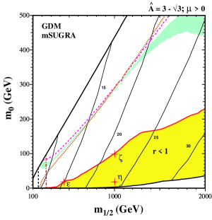
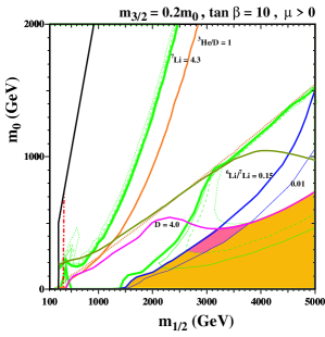
Figure 1: The left (first) panel shows the $(m_{0},m_{1/2})$ plane for mSUGRA with a gravitino LSP and stau NLSP, assuming $A_{0}=3-\sqrt{3}$, with the regions allowed by astrophysical constraints on stau decays Bench3 shaded light (yellow). The values of $\tan\beta$ are fixed by the vacuum conditions with the values indicated along the solid black contours, and the three benchmark points $\epsilon$, $\eta$ and $\zeta$ are shown by red $+$ signs. The right (second) panel shows the $(m_{0},m_{1/2})$ plane in the CMSSM, assuming fixed $\tan\beta=10$, with the regions allowed in the presence of cosmological bound-state effects and stau decays if $m_{\widetilde{G}}=0.2m_{0}$ shaded light (yellow). In the darker (pink) shaded region, bound-state effects yield ^6,7Li abundances in the ranges favoured by astrophysical observations. The new benchmark point $\theta$ is located in this ^6,7Li-friendly region Cyburt06 .

Table 1: The four benchmark points with gravitino DM and a $\tilde{\tau}_{1}$ NLSP that are considered in this paper. The quoted slepton, squark, gluino and the neutralino mass spectra (in GeV) have been calculated with ISAJET 7.74, using $m_{t}=175$ GeV.

Model	$\epsilon$	$\zeta$	$\eta$	$\theta$
$m_{0}$	20	100	20	330
$m_{1/2}$	440	1000	1000	3000
$A_{0}$	-25	-127	-25	0
tan$\beta$	15	21.5	23.7	10
sign($\mu$)	+1	+1	+1	+1
$\tilde{e}_{L},\tilde{\mu}_{L}$	303	676	669	1982
$\tilde{e}_{R},\tilde{\mu}_{R}$	168	382	369	1140
$\tilde{\nu}_{e},\tilde{\nu}_{\mu}$	289	666	659	1968
$\tilde{\tau}_{1}$	154	346	327	1140
$\tilde{\tau}_{2}$	304	666	659	1966
$\tilde{\nu}_{\tau}$	284	651	643	1944
$\tilde{u}_{L},\tilde{c}_{L}$	935	1992	1989	5499
$\tilde{u}_{R},\tilde{c}_{R}$	902	1913	1910	5248
$\tilde{d}_{L},\tilde{s}_{L}$	938	1994	1991	5500
$\tilde{d}_{R},\tilde{s}_{R}$	899	1903	1900	5217
$\tilde{t}_{1}$	703	1534	1541	4285
$\tilde{t}_{2}$	908	1857	1855	5130
$\tilde{b}_{1}$	858	1823	1819	5104
$\tilde{b}_{2}$	894	1874	1867	5203
$\tilde{g}$	1023	2187	2186	6089
$\tilde{\chi}_{1}^{0}$	179	425	424	1336
$\tilde{\chi}_{2}^{0}$	337	802	802	2467
$\tilde{\chi}_{1}^{\pm}$	338	804	804	2472

Recently, bound-state effects on light-element abundances in models with metastable stau NLSPs have been studied in several variants of the MSSM Cyburt06 ; Pradler06 , including mSUGRA and some other models in which its relations between $m_{\tilde{G}}$ and $m_{0}$ and between $A_{0}$ and $B_{0}$ are relaxed, but where universality is maintained for the soft SUSY-breaking parameters, a framework we term the constrained MSSM (CMSSM). The bound-state effects restrict greatly the allowed regions of parameter space, but one example was found within the CMSSM of an $(m_{1/2},m_{0})$ plane with $m_{\tilde{G}}=0.2m_{0}$ and $\tan\beta=10$, that has a wedge compatible with BBN and also a small region where the BBN predictions for the ^6,7Li abundances could be brought into better agreement with astrophysical observations. We propose and study here a new benchmark point in this ^6,7Li-friendly region, denoted by $\theta$, with the parameter choices shown in the last column of Table 1. Also shown in this column are some sparticle masses: like the rest of the ^6,7Li-friendly region, benchmark $\theta$ features relatively heavy sparticles beyond the reach of either the LHC or the ILC, but within the kinematic reach of CLIC.

In this connection we note that for benchmark $\theta$ the direct stau pair production cross section is $2.7\times 10^{-6}$ pb at the LHC with $\sqrt{s}=14$ TeV and $2.8\times 10^{-5}$ pb at the DLHC with $\sqrt{s}=28$ TeV. The plausible integrated luminosity of $10^{5}$ pb^-1 for the LHC would be insufficient to reach this point, and it would be very marginal at the SLHC with $10^{6}$ pb^-1. The only alternative to CLIC would be the DLHC with a very high integrated luminosity.

The bound-state effects depend sensitively on the stau lifetime, being much more important for longer lifetimes. This is why they would be unacceptable for the the stau in benchmark scenarios $\epsilon$, $\eta$ and $\zeta$, if it had the lifetime predicted by mSUGRA. However, as discussed in the following Section, the stau lifetime depends sensitively on the mass assumed for the gravitino. Hence, a CMSSM variant with similar masses for the masses of the spartners of the Standard Model particles but a smaller gravitino mass would not be excluded a priori on the basis of bound-state effects. For this reason, and since the previous benchmarks $\epsilon$, $\eta$ and $\zeta$ represent to a great extent the range of possibilities open to the ILC (limits on metastable particles exclude a stau much lighter than at benchmark $\epsilon$, and sparticles would be inaccessible to the LHC or ILC if they weighed much more than at points $\eta$ and $\zeta$), we continue to include all these points in the subsequent discussion, though our primary interest will be in the new ^6,7Li-friendly point $\theta$.

III The $\widetilde{\tau}_{1}$ NLSP Decay and Lifetime

Since we assume the conservation of R-parity, the gravitino must be produced at the end of any decay chain initiated by the decay of a heavy unstable supersymmetric particle. As already remarked, in models with universal scalar soft supersymmetry-breaking masses, the lightest slepton is generically the lighter stau mass eigenstate, the $\widetilde{\tau}_{1}$, as a result of renormalization-group effects and left-right sfermion mixing. In large regions of mSUGRA parameter space, the $\widetilde{\tau}_{1}$ is the NLSP, and is the penultimate sparticle in (essentially) every decay chain.

The $\widetilde{\tau}_{1}$ is in general a linear combination of $\widetilde{\tau}_{L}$ and $\widetilde{\tau}_{R}$, which are the superpartners of the left- and right-handed $\tau$ leptons $\tau_{L}$ and $\tau_{R}$, respectively. In general the stau mass eigenstates are

$$\widetilde{\tau}_{1} =\widetilde{\tau}_{L}\cos\theta_{\tilde{\tau}}+\widetilde{\tau}_{R}\sin\theta_{\tilde{\tau}},$$ (1)

$$\widetilde{\tau}_{2} =-\widetilde{\tau}_{L}\sin\theta_{\tilde{\tau}}+\widetilde{\tau}_{R}\cos\theta_{\tilde{\tau}},$$ (2)

where $\theta_{\tilde{\tau}}$ is the stau mixing angle, which is given by

$$\cos\theta_{\tilde{\tau}}=\frac{-m_{\tau}(A_{\tau}-\mu\tan\beta)}{\sqrt{(m_{\tilde{\tau}_{L}}^{2}-m_{\tilde{\tau}_{1}}^{2})+m_{\tau}^{2}(A_{\tau}-\mu\tan\beta)^{2}}},$$ (3)

where $|\cos\theta_{\tilde{\tau}}|>1/\sqrt{2}$ if $m_{\widetilde{\tau}_{L}}<m_{\widetilde{\tau}_{R}}$ and $|\cos\theta_{\tilde{\tau}}|<1/\sqrt{2}$ if $m_{\widetilde{\tau}_{R}}<m_{\widetilde{\tau}_{L}}$.

The interactions of the stau states $\widetilde{\tau}_{L,R}$ with the gravitino $\widetilde{G}$ and tau lepton $\tau$ are described by the Lagrangian Buchmuller04

$$L_{\widetilde{\tau}\tau\tilde{G}} = -\frac{1}{\sqrt{2}M_{P}}\left[(D_{\nu}\widetilde{\tau}_{L})^{*}\overline{\widetilde{G}}^{\mu}\gamma^{\nu}\gamma_{\mu}P_{L}\tau+(D_{\nu}\widetilde{\tau}_{L})\overline{\tau}P_{L}\gamma_{\mu}\gamma^{\nu}\widetilde{G}^{\mu}\right.$$ (4)

$$\left.+(D_{\nu}\widetilde{\tau}_{R})^{*}\overline{\widetilde{G}}^{\mu}\gamma^{\nu}\gamma_{\mu}P_{R}\tau+(D_{\nu}\widetilde{\tau}_{R})\overline{\tau}P_{R}\gamma_{\mu}\gamma^{\nu}\widetilde{G}^{\mu}\right],$$

where $D_{\nu}\equiv(\partial_{\nu}+ig_{e}A_{\nu})$, with $A_{\nu}$ denoting the gauge boson and $M_{P}\equiv(8\pi G_{N})^{-1/2}=2.436\times 10^{18}$ GeV is the reduced Planck mass, with the Newton constant $G_{N}=6.707\times 10^{-39}$ GeV^-2.

The stau decay rate is dominated by the two-body decay into tau and gravitino ($\widetilde{\tau}_{1}\rightarrow\tau\widetilde{G}$), and the decay width of the $\widetilde{\tau}_{1}$ is given by

$$\Gamma_{\widetilde{\tau_{1}}}=\frac{(m_{\widetilde{\tau}_{1}}^{2}-m_{\widetilde{G}}^{2}-m_{\tau}^{2})^{4}}{48\pi M_{p}^{2}m_{\widetilde{G}}^{2}m_{\widetilde{\tau}_{1}}^{3}}\left(1-\frac{4m_{\widetilde{G}}^{2}m_{\tau}^{2}}{(m_{\widetilde{\tau}_{1}}^{2}-m_{\widetilde{G}}^{2}-m_{\tau}^{2})^{2}}\right)^{3/2},$$ (5)

where $m_{\widetilde{\tau}_{1}}$, $m_{\widetilde{G}}$ and $m_{\tau}$ are the masses of the stau $\widetilde{\tau}_{1}$, gravitino $\widetilde{G}$ and tau lepton $\tau$, respectively. As illustrative examples, if we take $m_{\widetilde{\tau}_{1}}=150$ GeV (similar to the mass at benchmark point $\epsilon$), we find a lifetime of $\Gamma_{\widetilde{\tau_{1}}}^{-1}=7762$ s (25.9 years) for a gravitino mass of $m_{\widetilde{G}}=1$ GeV (100 GeV), respectively. The lifetime and decay width of the stau as functions of the gravitino mass for various stau mass values are presented in Fig. 2.

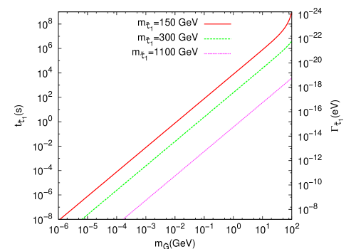
Figure 2: The stau NLSP lifetime and decay width as functions of the gravitino mass, for various choices of stau mass.

Neglecting the tau lepton mass, the mean stau decay length, obtained from the relation $L=\beta\gamma t_{\tilde{\tau}}$, is shown in Fig. 3. For instance, taking $\beta\gamma=1$ and $m_{\widetilde{G}}=1$ MeV would imply a mean decay length of $L=2.33\times 10^{6}$ m ($L=109.6$ m) for $m_{\tilde{\tau_{1}}}=150$ GeV ($m_{\tilde{\tau_{1}}}=1100$ GeV), respectively. Only for $m_{\widetilde{G}}<1$ KeV might a typical stau with $\beta\gamma={\cal O}(1)$ decay within a generic collider detector. In this case the light gravitino would constitute either warm or even hot dark matter, which is disfavoured by the modelling of cosmological structure formation.

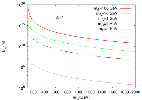
Figure 3: The mean decay length of the stau NLSP as a function of its mass, for various choices of the gravitino mass.

However, some fraction of the staus may be produced with velocities sufficiently low that strong ionization energy loss causes them to stop within the detector. In such a case, interesting information may be extracted from the stau decays. For example, the mass of the gravitino produced in the decay could in principle be inferred kinematically from the relation $m_{\widetilde{G}}^{2}=m_{\tilde{\tau}_{1}}^{2}+m_{\tau}^{2}-2m_{\tau}E_{\tau}$, unless it is very small. Also, we note that the polarization of the tau produced in the stau decay must coincide with the combination of ${\tilde{\tau}_{L,R}}$ contained in the ${\tilde{\tau}_{1}}$, offering in principle the possibility of determining the stau mixing angle $\theta_{\tilde{\tau}}$ by examining the kinematical distributions in the subsequent tau decays, as well as in the polarization dependence of stau pair production. We discuss later the prospects for measuring $\theta_{\tilde{\tau}}$ using the stau pair-production cross section in $e^{+}e^{-}$ collisions.

The point $\epsilon$ is near the tip of the wedge in Fig. 1, and the stau NLSP $\tilde{\tau}_{1}$ has a mass of $m_{\tilde{\tau}}=154$ GeV and a lifetime of $t_{\tilde{\tau}}=2.9\times 10^{6}$ s in mSUGRA ² . The benchmark point $\zeta$ is close to the upper edge of the wedge, with $m_{0}=100$ GeV and $\tan\beta\simeq 21.5$, and the $\tilde{\tau}_{1}$ has a mass of $346$ GeV and a lifetime of $1.7\times 10^{6}$ s in mSUGRA. The benchmark point $\eta$ is close to the lower edge of the wedge in Fig. 1, with $m_{0}=20$ GeV and $\tan\beta=23.7$. Here the $\tilde{\tau}_{1}$ has a mass of $m_{\tilde{\tau}}=327$ GeV and a smaller lifetime of $6.4\times 10^{4}$ s in mSUGRA. The new benchmark point $\theta$ introduced here with a much larger value of $m_{1/2}$, corresponding to $m_{\tilde{\tau}}=1140$ GeV and $t_{\tilde{\tau}}=1.4\times 10^{3}$ s. The stau mixing angle $\theta_{\tilde{\tau}}$ takes the following values at these points: $77.2^{o}$, $82.4^{o}$, $81.8^{o}$ and $89.0^{o}$ for the points $\epsilon$, $\zeta$, $\eta$ and $\theta$, respectively. Thus, each of these scenarios predicts that the ${\tilde{\tau}_{1}}$ should be mainly right-handed. Then, the right-handed polarization of the electron beam enhances the $\tilde{\tau}_{1}^{+}\tilde{\tau}_{1}^{-}$ signal. We expect this feature to be quite general, and more marked for heavier staus. Correspondingly, the tau produced in stau decay should also be mainly right-handed.

IV Production of Stau Pairs in $e^{+}e^{-}$ Annihilation

The reaction $e^{+}e^{-}\rightarrow\tilde{\tau}_{1}^{+}\tilde{\tau}_{1}^{-}$ proceeds via direct-channel $\gamma$ and $Z$ exchange as shown in Fig. 4. The tree-level vertex factors can be parametrized as given in Table 1 for the stau-photon-stau ($\widetilde{\tau}_{1}^{+}\gamma\tilde{\tau}_{1}^{-}$) and stau-Z-stau ($\widetilde{\tau}_{1}^{+}Z\tilde{\tau}_{1}^{-}$) interactions.

Figure 4: The tree-level Feynman diagrams for the reaction $e^{+}e^{-}\rightarrow\tilde{\tau}_{1}^{+}\tilde{\tau}_{1}^{-}$.

Table 2: The vertices for $\widetilde{\tau}_{1}\tau\widetilde{G}$, $\widetilde{\tau}_{1}^{+}\tilde{\tau}_{1}^{-}\gamma$ and $\widetilde{\tau}_{1}^{+}\tilde{\tau}_{1}^{-}Z$ interactions and the corresponding tree-level diagrams. The parameters $C_{L,R}$ depend on the stau mixing angle $\theta_{\tilde{\tau}}$ and the coefficients $C_{1,2}$ depend also on the weak mixing angle. $F$ is the supersymmetry breaking scale.

		$\frac{1}{2F}\left[(\not p_{2}\not p_{3}+\not p_{3}\not p_{2})[C_{L}(1-\gamma_{5})+C_{R}(1+\gamma_{5}]\right]$
		$ig_{e}(p_{3\mu}-p_{2\mu})$
		$-\frac{ig_{e}}{\sin 2\theta_{W}}(C_{1}p_{3\mu}+C_{2}p_{2\mu})$

The cross section for the process $e^{+}e^{-}\to\tilde{\tau}_{1}^{+}\tilde{\tau}_{1}^{-}$ with a left (L)- or right (R)-polarized $e^{\pm}$ beams at a center-of-mass energy $\sqrt{s}$ is given by kraml99 .

$$\sigma = \frac{\pi\alpha^{2}\beta^{3}}{3s}\left[(1-P_{-}P_{+})+\frac{I_{3}\cos^{2}\theta_{\tilde{\tau}}+\sin^{2}\theta_{W}}{2\cos^{2}\theta_{W}\sin^{2}\theta_{W}}[v_{e}(1-P_{-}P_{+})-a_{e}(P_{-}-P_{+})]P_{\gamma Z}\right.$$ (6)

$$+ \left.\frac{(I_{3}\cos^{2}\theta_{\tilde{\tau}}+\sin^{2}\theta_{W})^{2}}{16\cos^{4}\theta_{W}\sin^{4}\theta_{W}}[(v_{e}^{2}+a_{e}^{2})(1-P_{-}P_{+})-2v_{e}a_{e}(P_{-}-P_{+})]P_{ZZ}\right],$$

where $v_{e}=4\sin^{2}\theta_{W}-1$ and $a_{e}=-1$. $P_{-}$ and $P_{+}$ denote the degree of polarization of the $e^{-}$ and $e^{+}$ beams, respectively. The propagator terms are given by

$$P_{ZZ}=\frac{s^{2}}{(s-m_{Z}^{2})^{2}+m_{Z}^{2}\Gamma_{Z}^{2}}\quad,\qquad P_{\gamma Z}=\frac{s(s-m_{Z}^{2})}{(s-m_{Z}^{2})^{2}+m_{Z}^{2}\Gamma_{Z}^{2}}$$ (7)

The cross sections with unpolarized electron and positron beams in the four benchmark scenarios, shown in Fig. 5, exhibit a typical $\beta^{3}$ threshold suppression, where $\beta\equiv\sqrt{1-4m_{\tilde{\tau}}^{2}/s}$. Illustrative values of the cross sections for producing $\tilde{\tau}_{1}$ pairs in the benchmark scenarios $\epsilon,\zeta,\eta$, and $\theta$ are shown in Table 3, for center-of-mass energies between 0.5 and 5 TeV. As an example, with an integrated luminosity $L_{int}=200$ fb^-1 at $\sqrt{s}=1$ TeV, the benchmark points $\epsilon,\zeta$ and $\eta$ would produce 4882, 1846 and 2150 $\tilde{\tau}_{1}$ pairs, respectively. In general, the peak cross sections are found at center-of-mass energies $\sqrt{s}\simeq 3m_{\tilde{\tau}_{1}}$, namely $\sqrt{s}\simeq 500,1000$ and 4000 GeV for benchmarks $\epsilon$, $\eta$ and $\zeta$, and $\theta$, respectively. These would be good energies for high-statistics studies of stau properties. The mass of the $\tilde{\tau}$ can be estimated from the threshold scan and the mixing angle from the polarized cross sections.

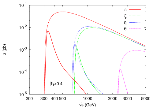
Figure 5: The dependences of the tree-level cross sections for $\tilde{\tau}_{1}$ pair production on the linear-collider center-of-mass energy, as calculated using PYTHIA and ISASUGRA. We also show the cross sections for producing slow staus with $\beta\gamma<0.4$ in the various benchmark scenarios, also as functions of the center-of-mass energy of the linear $e^{+}e^{-}$ collider. The optimal energies for obtaining the largest numbers of these stoppable staus are different from the energies where the maxima of the pair-production cross sections appear.

Table 3: The total cross section in pb calculated using PYTHIA with the full ISASUGRA spectrum, including both initial- and final-state radiation (ISR+FSR).

	Benchmark points	$\epsilon$	$\zeta$	$\eta$	$\theta$
	$m_{\tilde{\tau}_{1}}$(GeV) $=$	154	346	327	1140
	500	$4.799\times 10^{-2}$	$-$	$-$	-
$\sqrt{s}$(GeV)	1000	$2.441\times 10^{-2}$	$9.230\times 10^{-3}$	$1.075\times 10^{-2}$	-
	3000	$3.665\times 10^{-3}$	$3.142\times 10^{-3}$	$3.197\times 10^{-3}$	$7.235\times 10^{-4}$
	5000	$1.432\times 10^{-3}$	$1.299\times 10^{-3}$	$1.311\times 10^{-3}$	$7.889\times 10^{-4}$

The unpolarized cross sections shown in Fig. 6 have non-trivial dependencies on the stau mixing angle $\theta_{\tilde{\tau}}$. We see that the cross sections exhibit minima as functions of $\theta_{\tilde{\tau}}$ when $\cos\theta_{\tilde{\tau}}\sim 0.6$, due to the interference of $\gamma$ and $Z$ exchange. One might hope to use this dependence to extract the stau mixing angle. Unfortunately, the dependencies of the unpolarized cross sections on $\theta_{\tilde{\tau}}$ are minimized when $\cos\theta_{\tilde{\tau}}\sim 0$, which corresponds to a mainly right-handed stau and is the region expected theoretically, as discussed in the previous section. Moreover, there is a twofold ambiguity in the determination of $\theta_{\tilde{\tau}}$, with the alternative value corresponding to the ${\tilde{\tau}_{1}}$ being predominantly left-handed. Considering the case $m_{\tilde{\tau}_{1}}=154.0$ GeV, similar to the mass at the reference point $\epsilon$, and assuming $\cos\theta_{\tilde{\tau}}=0.60$, for which the cross section exhibits a minimum and hence no left/right ambiguity, without radiation effects we find unpolarized cross sections of $48.3\pm 0.5$ pb and $21.3\pm 0.3$ pb for $\sqrt{s}=500$ GeV and $\sqrt{s}=1000$ GeV with $L_{int}=200$fb^-1, respectively, where the errors are statistical. As seen in Fig. 6, these errors on the unpolarized cross-section measurement would not provide an accurate determination of $\cos\theta_{\tilde{\tau}}$ or of the stau handedness.

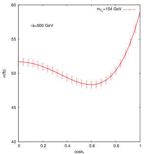
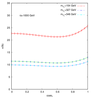
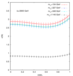
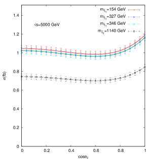
Figure 6: The unpolarized cross sections for $e^{+}e^{-}\rightarrow\tilde{\tau}_{1}^{+}\tilde{\tau}_{1}^{-}$ in fb at $\sqrt{s}=500,1000,3000$ and $5000$ GeV as a function of the stau mixing angle $\theta_{\tilde{\tau}}$ for four of the benchmark scenarios. The expected statistical errors in the cross section measurement are shown for different benchmark points. We take the integrated luminosities $L_{int}=200$ fb^-1 (for $\sqrt{s}=500$ GeV), $200$ fb^-1 (for $\sqrt{s}=1000$ GeV), $400$ fb^-1 (for $\sqrt{s}=3000$ GeV) and $1000$ fb^-1 (for $\sqrt{s}=5000$ GeV) for the ILC and CLIC energy options.

One way of determining the handedness of the ${\tilde{\tau}_{1}}$ is the $\tau$ decay polarization measurement, as mentioned previously. More detailed analysis of the measurement of tau lepton polarization in hadronic decay channels has been studied in Nojiri95 ; Godbole05 ; Choi07 . The angular distribution of the pion from polarized tau lepton can be expressed as $d\Gamma/\Gamma dz=(1+P_{\tau}z)/2$, where $P_{\tau}$ being the polarization of the $\tau$ lepton. The decay $\tilde{\tau}_{1}\to\tau\tilde{G}$ implies $P_{\tau}=\sin^{2}\theta_{\tau}-\cos^{2}\theta_{\tau}$. For the points $\epsilon,\zeta,\eta$ and $\theta$ we have $P_{\tau}=$$0.902$, $0.965$, $0.959$ and $0.999$, respectively. The energy distributions of the pions show a maximum in which the minimum of tau energy can be measured. The fraction of the momenta $p_{\pi^{\pm}}/p_{\tau-jet}$ can be calculated from the measurements of pion momentum from tracker and tau-jet momentum from the calorimetric energy deposition. Another would be to use a polarized $e^{\pm}$ beams. As we can see from Fig. 7, the polarization of the $e^{\pm}$ beam would offer the possibility of measuring the stau mixing angle (and the stau mass) with much greater accuracy. Moreover, it can be used to enhance the signal and reduce the backgrounds. The signal is the same flavor, opposite sign taus with missing transverse momentum $\not{p}_{T}$. The SM backgrounds consists of $\tau^{+}\tau^{-}+\not{p}_{T}$ from the pair production of $W$-bosons and $Z$-bosons as well as the single production $Z+\not{p}_{T}$. The total cross section for $W^{+}W^{-}$ production is large compared to typical supersymmetry cross sections, however it proceeds via t-channel exchange of the neutrino, and hence it is very forward peaked. This background can be much suppressed by using a right-handed polarized electron beam and appropriate cuts Khotilovich05 . Here we note that one can combine the measurements via threshold scan and polarized cross sections as well as the tau polarization to complete the determination of the SUGRA model parameters.

In particular, as seen in Fig. 7, even a simple measurement of the ratio of the cross section with left- and right-polarized $e^{\pm}$ beams would remove the ambiguity between the left- and right-handed stau solutions for the total unpolarized cross section measurement that was noted above. Indeed, measurements of the cross sections with $e^{\pm}_{L/R}$ beams could determine both $\cos\theta_{\tilde{\tau}}$ and $m_{\tilde{\tau}_{1}}$ with interesting accuracy. We display in Fig. 8 the error bands in the $(m_{\tilde{\tau}_{1}},\cos\theta_{\tilde{\tau}})$ obtained from measurements of the polarized cross sections for $e^{+}e^{-}\to\tilde{\tau}_{1}^{+}\tilde{\tau}_{1}^{-}$ at $\sqrt{s}=500,1000,3000$ GeV. The combined experimental accuracies in the mass and mixing angle of the stau obtained from this Monte Carlo simulation are $m_{\tilde{\tau}_{1}}=154.0\pm 0.7$ GeV and $\Delta\cos{\theta}_{\tilde{\tau}}=0.005$, respectively. Similar analysis yield $m_{\tilde{\tau}_{1}}=346.0\pm 2.4$ GeV, $\Delta\cos{\theta}_{\tilde{\tau}}=0.01$ and $m_{\tilde{\tau}_{1}}=327.0\pm 2.4$ GeV, $\Delta\cos{\theta}_{\tilde{\tau}}=0.01$ using measurements at $\sqrt{s}=1000$ GeV and $m_{\tilde{\tau}_{1}}=1140\pm 13$ GeV and $\Delta\cos{\theta}_{\tilde{\tau}}=0.03$ using measurements at $\sqrt{s}=3000$ GeV, for the points $\zeta$, $\eta$ and $\theta$, respectively. Here, we take the integrated luminosities $L_{int}=200$ fb^-1 for $\sqrt{s}=500$(or $1000$) GeV and $L_{int}=400$ fb^-1 for $\sqrt{s}=3000$ GeV. For a high luminosity option ($L_{int}=1000$ fb^-1) for the CLIC with $\sqrt{s}=3000$ GeV, the stau $\tilde{\tau}_{1}$ can be measured with less errors on the mass and mixing, namely $\Delta m_{\tilde{\tau}}=8$ GeV and $\Delta\cos{\theta}_{\tilde{\tau}}=0.02$ at the point $\theta$. In our calculations, we take into account the degree of polarization $P_{-}=90\%$ for the electron (which means 90% of the electrons are left-polarized and the rest is unpolarized) and $P_{+}=60\%$ for the positron. It might be possible to reduce further the error in $m_{\tilde{\tau}_{1}}$ by using tracking and time-of-flight measurements, as has been considered for the LHC, but we see from Fig. 8 that this would be unlikely to improve significantly the determination of $\cos\theta_{\tilde{\tau}}$.

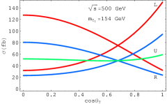
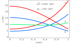
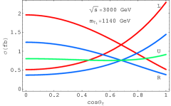
Figure 7: The cross section of $e^{+}e^{-}\rightarrow\tilde{\tau}_{1}^{+}\tilde{\tau}_{1}^{-}$ in fb at $\sqrt{s}=500,1000$ and $3000$ GeV as a function of the stau mixing angle $\theta_{\tilde{\tau}}$, for unpolarized (U) as well as 90% left- (L) and 90% right- (R) polarized $e^{-}$ beams, and assuming $m_{\tilde{\tau}_{1}}=154,346,327$ and $1140$ GeV for the benchmark points. The red lines show the results for both the electron (90%) and positron (60%) polarized, while blue lines show only electrons (90%) are polarized. The statistical experimental errors would be similar to those shown in Fig. 6.

Figure 8: The error bands for $\cos\theta_{\tilde{\tau}}$ as a function of the stau mass, as obtained from measurements of the cross sections for $e^{+}e^{-}\rightarrow\tilde{\tau}_{1}^{+}\tilde{\tau}_{1}^{-}$ at $\sqrt{s}=500,1000,3000$ GeV with left (90%)- (L), right (90%)- (R) and unpolarized (U) $e^{-}$ beams, assuming for inputs $m_{\tilde{\tau}_{1}}=154,346,327$ and $1140$ GeV, as for the point $\epsilon,\zeta,\eta,\theta$, and the value of $\cos\theta_{\tilde{\tau}}=0.60$. Here we take the positron polarization (60%) opposite of electron polarization.

V Detection of Stau Decays

Measuring stau decays using staus that stop and decay inside a linear-collider detector was first discussed in Martyn06 . Measurement of, e.g., the mass of the gravitino and the decay tau polarization require optimizing the number of staus stopped and then decaying inside the collider detector, which we discuss here. As in Martyn06 , we assume a future linear-collider detector with the structure proposed in TESLA01 . A metastable stau may stop in the hadron calorimeter or in the iron yoke. The amount of absorber material $R$(g/cm²) in the detector, summed along the radial direction at different longitudinal angles, is 835 to 1250 g/cm² for the hadronic calorimeter (HCAL) and 1810 to 2750 g/cm² for the magnet return yoke, respectively. As discussed in Martyn06 , the range $R$ of a metastable stau with given $\beta\gamma$ and mass $m_{\tilde{\tau_{1}}}$ is given by

$$log_{10}(\beta\gamma)\;=\;\frac{\left[log_{10}(R/m_{\tilde{\tau_{1}}})-c_{1}\right]}{c_{2}},$$ (8)

where $c_{1}=2.087$ and $c_{2}=3.227$ for steel Rossi52 . The corresponding values of $\beta\gamma$ for staus stopping in different detector parts for the benchmark points are shown in Table 4. (The corresponding values for some other stau masses are given in Table II of Martyn06 .) As a representative example, we consider below the production of slow-moving staus with $\beta\gamma<0.4$, that might plausibly be stopped with a linear-collider detector, so that their decays could be observed.

Table 4: The maximal values of $\beta\gamma$ below which staus would be stopped in different detector parts, for the benchmark scenarios $\epsilon,\eta,\zeta$ and $\theta$.

$m_{\tilde{\tau}}$ (GeV)	$\beta\gamma$ (HCAL)	$\beta\gamma$ (Iron Yoke)
154	0.38-0.43	0.48-0.55
346	0.30-0.34	0.38-0.43
327	0.30-0.34	0.38-0.44
1140	0.21-0.23	0.26-0.30

In the absence of photon radiation, the velocity of the outgoing staus in the direct pair-production reaction $e^{+}e^{-}\rightarrow\tilde{\tau}_{1}^{+}\tilde{\tau}_{1}^{-}$ is simply $\beta=\sqrt{1-4m_{\tilde{\tau}}^{2}/s}$. However, the values of the stau velocities are altered when initial-state radiation and a realistic luminosity spectrum are taken into account. Fig. 9 shows the distributions of $\beta\gamma$ expected for the $\tilde{\tau}_{1}$s pair-produced in the various gravitino DM scenarios at the center-of-mass energies 500 GeV (the design for the ILC), 1 TeV and 3 TeV (the design for CLIC). The two sets of $\beta\gamma$ distributions correspond to alternative luminosity spectra yielded by beam conditions designed to optimize the luminosity close to the nominal center-of-mass energy (left) and the total luminosity (right). We see that the $\beta\gamma$ distributions exhibit substantial low-energy tails, particularly in the case where the total luminosity is optimized, as shown in the right panel of Fig. 9.

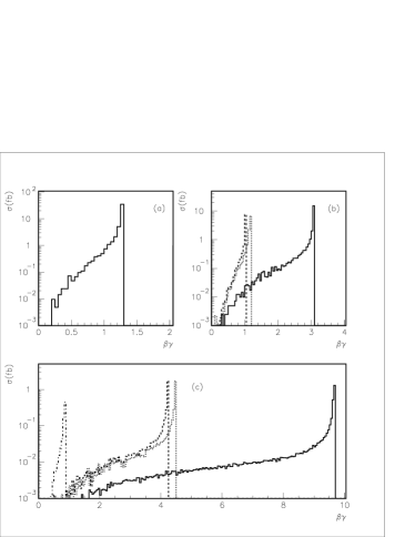
Figure 9: The $\beta\gamma$ distributions for direct stau pair-production $e^{+}e^{-}\rightarrow\tilde{\tau}_{1}^{+}\tilde{\tau}_{1}^{-}$ at different center-of-mass energies: a) $\sqrt{s}=500$ GeV, b) $\sqrt{s}=1000$ GeV and c) $\sqrt{s}=3000$ GeV. The solid, dashed, dotted and dashed-dotted lines correspond to the gravitino DM points $\epsilon$, $\zeta$, $\eta$ and $\theta$, respectively. These distributions were obtained from simulations of running conditions designed (left) to optimize the luminosity close to the nominal center-of-mass energy and (right) to optimize the total luminosity. The low-energy tails of the $\beta\gamma$ distributions are apparent, and much larger in the right-hand panel. Here, we have used the CALYPSO library Daniel01 to include the luminosity spectrum into the event generator PYTHIA.

We plot in Fig. 5 the cross sections the production of staus with $\beta\gamma<0.4$ via direct pair-production $e^{+}e^{-}\rightarrow\tilde{\tau}_{1}^{+}\tilde{\tau}_{1}^{-}$ accompanied by initial- and final-state radiation, which opens up the possibility of producing slow-moving staus. We see that the optimal center-of-mass energies for producing slow-moving staus via direct pair-production are 330, 730, 700 and 2500 GeV for benchmarks $\epsilon,\zeta,\eta$ and $\theta$, respectively. We note that the center-of-mass energy dependencies of these cross sections for slow-moving staus are completely different from the total cross sections shown in Fig. 5, reflecting the increasing difficulty of radiating sufficiently to produce a slow-moving stau as the center-of-mass energy increases.

Table 5 gives estimates of the numbers of staus with $\beta\gamma<0.4$, as produced directly via $e^{+}e^{-}\rightarrow\tilde{\tau}_{1}^{+}\tilde{\tau}_{1}^{-}$ accompanied by initial- and final-state radiation at selected nominal center-of-mass energies. These staus might stop in a typical linear-collider detector, where their decays could then be observed. We note that the numbers of stopped staus obtained at the optimal center-of-mass energies for benchmark points are more than an order of magnitude larger than the numbers that would be stopped in measurements at center-of-mass energies corresponding (approximately) to the peaks of the total pair-production cross sections, namely 500, 1000, 1000 and 3000 GeV, respectively.

Table 5: The numbers of staus with $\beta\gamma<0.4$, that may be stopped in a generic linear-collider detector, for the different benchmark points at different center-of-mass energies and luminosities. In the fourth column, the energies are optimized for the direct pair-production of slow-moving staus, whereas in the last column all sparticle pair-production cross sections are included.

$\sqrt{s}$(GeV)	$500$	$1000$	$3000$	Optimal for	Maximal including
$L_{int}$(fb-1)	200	200	400(1000)	pair prod’n	other prod’n processes
$\epsilon$	34	4	4(10)	1500	1700
$\zeta$	-	12	4(10)	254	700
$\eta$	-	10	4(10)	370	600
$\theta$	-	-	8(20)	56(140)	140(350)

VI Indirect Stau Production

In addition to direct stau pair-production $e^{+}e^{-}\rightarrow\tilde{\tau}_{1}^{+}\tilde{\tau}_{1}^{-}$, staus can be produced via the cascade decays of heavier sparticles, e.g. sleptons, $\tilde{e}_{R}\to\tilde{\tau}_{1}\tau e$, or neutralinos, $\tilde{\chi}_{1}^{0}\to\tilde{\tau}_{1}\tau$. Each heavier sparticle eventually yields one stau among its cascade decay products, which later decays into a gravitino. For example, for the nominal ILC center-of-mass energy of $\sqrt{s}=500$ GeV, the most important contributions to stau-pair production at point $\epsilon$ in fact come from the processes $e^{+}e^{-}\to\tilde{\chi}_{1}^{0}\tilde{\chi}_{1}^{0}$ and $e^{+}e^{-}\to\tilde{e}_{R}^{+}\tilde{e}_{R/L}^{-}$ with cross sections of $1.26\times 10^{-1}$ pb and $7.44\times 10^{-2}/6.76\times 10^{-2}$ pb, respectively. On the other hand, for the point $\theta$ at $\sqrt{s}=3000$ GeV, the main contribution comes from the pair production of right-handed selectrons, smuons and neutralinos with the cross sections $8.49\times 10^{-4}$ pb, $7.31\times 10^{-4}$ pb and $9.66\times 10^{-4}$ pb, respectively. We display in Fig. 10 the dominant cross sections for sparticle pair-production in unpolarized $e^{+}e^{-}$ collisions in benchmarks $\epsilon,\eta,\zeta$ and $\theta$, as functions of the center-of-mass energy.

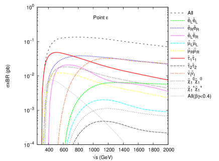
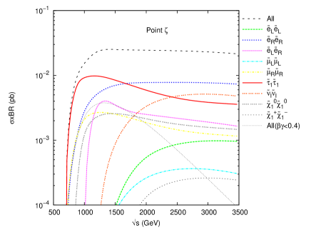
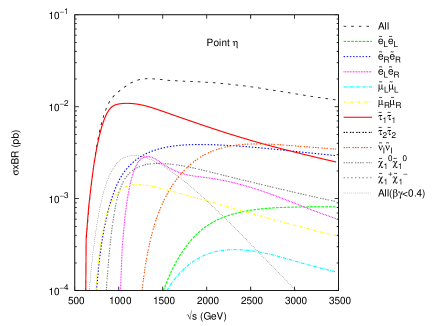
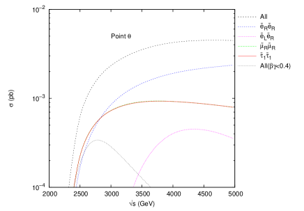
Figure 10: The cross sections for pair-production of supersymmetric particles in the benchmark scenarios $\epsilon,\zeta,\eta$ and $\theta$, as functions of the $e^{+}e^{-}$ center-of-mass energy. Also shown are the yields of slow-moving staus with $\beta\gamma<0.4$.

The pair-production of these heavier sparticles would be interesting in its own right, providing new opportunities to study sparticle spectroscopy with high precision, and to measure many sparticle decay modes. Some prominent decay modes of selectrons, smuons, neutralinos, charginos and heavier staus are shown in Table 6 ³: measuring these would give much information about sparticle masses and couplings, and hence the underlying pattern of supersymmetry breaking.

Table 6: Significant decay modes and branching ratios of selectrons, smuons, neutralinos, charginos and heavy staus for the chosen benchmark points $\epsilon$,$\zeta$,$\eta$ and $\theta$. Here, the charged lepton $l^{-}$ may be either $e^{-}$ or $\mu^{-}$, and the branching ratios add up to $\sim 100$ % when these and charge-conjugate modes are added.

Sparticle	Significant decay modes	BR (%) for $\epsilon$,$\zeta$,$\eta$,$\theta$
$\tilde{l}_{L}^{-}/\tilde{\nu}_{l}$	$\tilde{\chi}_{1}^{0}l^{-}/\tilde{\chi}_{1}^{0}\nu_{l}$	$100,100,100,100$
$\tilde{l}_{R}^{-}$	$\tilde{\tau}_{1}^{-}\tau^{+}l^{-}$	$45,42,40,0$
	$\tilde{\tau}_{1}^{+}\tau^{-}l^{-}$	$55,58,60,0$
	$\tilde{\tau}_{1}^{-}\bar{\nu}_{\tau}\nu_{l}$	$0,0,0,100$
$\tilde{\nu}_{\tau}$	$\tilde{\chi}_{1}^{0}\nu_{\tau}$	$55,21,17,64$
	$\tilde{\tau}_{1}^{-}W^{+}$	$45,79,83,36$
$\tilde{\tau}_{2}^{-}$	$\tilde{\chi}_{1}^{0}\tau^{-}$	$50,20,17,56$
	$\tilde{\tau}_{1}^{-}Z^{0}$	$23,37,39,16$
	$\tilde{\tau}_{1}^{-}H^{0}$	$27,43,44,28$
$\tilde{\chi}_{1}^{0}$	$\tilde{\tau}_{1}^{\pm}\tau^{\mp}$	$35,30,29,17$
	$\tilde{l}_{R}^{\pm}l^{\mp}$	$7,10,11,17$
$\tilde{\chi}_{1}^{-}$	$\tilde{\tau}_{1}^{-}\nu_{\tau}$	$13,4,5,0$
	$\tilde{\nu}_{l}l^{-}$	$18,16,16,17$
	$\tilde{l}^{-}\nu_{l}$	$9,13,14,16$
	$\tilde{\nu}_{\tau}\tau^{-}$	$22,19,19,18$
	$\tilde{\tau}_{2}^{-}\nu_{\tau}$	$8,15,15,17$
$\tilde{\chi}_{2}^{0}$	$\tilde{\tau}_{1}^{\pm}\tau^{\mp}$	$7,2,2,0$
	$\tilde{\nu}_{\tau}\bar{\nu}_{\tau}$/$\tilde{\bar{\nu}}_{\tau}\nu_{\tau}$	$10,10,10,9$
	$\tilde{\nu}_{l}\bar{\nu}_{l}$/$\tilde{\bar{\nu}}_{l}\nu_{l}$	$9,8,8,8$
	$\tilde{l}^{\pm}l^{\mp}$	$5,7,7,8$
	$\tilde{\tau}_{2}^{\pm}\tau^{\mp}$	$4,8,8,8$

Concerning the point $\theta$, the angular distributions of the staus and right-handed selectrons produced directly are given in Fig. 11. The staus peak around the central part of the distribution for their pair production while selectrons place forward direction for the $\tilde{e}^{+}_{R}\tilde{e}^{-}_{R}$ production due to the contribution from the neutralino exchange in the $t-$channel. If one study only the direct production of staus it is useful to apply a cut on the angular distribution $\cos\theta<2/3$ for an easy identification of staus. In this case the direct signal cross section reduces $15\%$ and the contribution from indirect production can be eliminated mostly. The right-handed smuons show the same angular distribution as the staus for their pair production. At this point, in order to be sure that stau is still an NLSP we need to have experimental identification of the corresponding final states. Assuming the stau is an NLSP we expect hadronic decay channels of tau leptons and the missing energy, otherwise smuons give their unique signatures in the muon spectrometer when they stopped inside the detector. However, here we take the stau as an NLSP with a good motivation from the BBN implications. We show in Fig. 10 all the contributions to the stau pairs from the indirect production mechanisms for the corresponding benchmark points. In addition, our interest here is in the contributions of these heavier sparticles to the total yields of slow-moving staus with $\beta\gamma<0.4$, which are also shown in Fig. 10. Comparing these yields with those produced by direct pair-production alone, shown in Fig. 5, we see that they are greatly enhanced. It is also apparent that the optimal center-of-mass energies are substantially higher, reflecting the higher thresholds for pair-producing heavier sparticles. Specifically, we find optimal center-of-mass energies of 430, 1200, 1150 and 2800 GeV for the benchmark points $\epsilon,\zeta,\eta$ and $\theta$, respectively. The last column of Table 5 displays the maximal number of slow-moving and hence stoppable staus that might be obtainable at these optimal center-of-mass energies in the four benchmark scenarios. These numbers provide greatly improved prospects for observing stau decays into gravitinos. This would yield direct insight into the mechanism of supersymmetry breaking, via a measurement of the stau lifetime, and possibly of the gravitino mass, via the kinematics of stau decays.

Figure 11: The angular distributions of the staus (solid line) and right-handed selectrons (dashed line) from their pair productions at the center of mass energy $\sqrt{s}=3000$ GeV.

VII Conclusion

We have discussed in this paper how the study of a metastable stau NLSP could be optimized at a linear collider such as the ILC or CLIC. The stau production rate, particularly using a polarized $e^{-}$ beam, would provide information on the handedness of the stau, as well as its mass. The center-of-mass energy could then be optimized for the combined direct and indirect production of slow-moving staus that would stop in the detector. Their decays could provide valuable information, not only on the stau lifetime and on the mass of the gravitino, but also supplementary information on the handedness of the stau via a measurement of the polarization of the tau decay products. The following are possible scenarios for studying metastable stau scenarios at the LHC and a subsequent linear collider.

If there is a metastable stau weighing up to $\sim 300$ GeV, as in benchmarks $\eta$ and $\zeta$, the LHC has been shown able to produce and detect them, and also to analyze the mSUGRA models in which they appear Ellis06 ; Hamaguchi06 . Specifically, it should be possible to measure the stau mass with an accuracy of $\sim 1$ %. However, most of the LHC staus would be produced with $\beta\gamma\sim 1$, and would decay outside the detector if they have lifetimes $>10^{-7}$ s. We recall that there are no significant cosmological constraints on such staus if their lifetimes $<1$ s, and that there are only weak constraints on staus with lifetimes $<10^{3}$ s. Therefore, collider information on the stau lifetime would be interesting for cosmology as well as the theory of supersymmetry breaking. However, the numbers of slow staus that stop inside the LHC detectors would be relatively modest: perhaps just a handful in benchmarks $\eta$ and $\zeta$, and somewhat more in benchmark $\epsilon$. The LHC would detect no staus in the case of benchmark $\theta$.

If the stau is indeed found by the LHC, in these scenarios one would know the optimal energy for producing the optimal number of stopping staus via the reaction $e^{+}e^{-}\to\tilde{\tau}_{1}^{+}\tilde{\tau}_{1}^{-}$. As we have emphasized in this paper, there would in general be many additional staus coming from the decays of heavier sparticles produced by reactions such as $e^{+}e^{-}\to\tilde{e}_{R}\tilde{e}_{L}$, $e^{+}e^{-}\to\chi\chi$, etc.. The masses of these heavier sparticles could also be measured at the LHC in models resembling benchmarks $\epsilon,\eta$ and $\zeta$, and hence the corresponding $e^{+}e^{-}$ thresholds could be estimated. These production mechanisms would also yield slow staus that should be included in the choice of the $e^{+}e^{-}$ center-of-mass energy in order to maximize the number of stopped staus.

Alternatively, the stau might be too heavy to be produced at the LHC, as in benchmark scenario $\theta$ which, we recall, has the added merit of being ^6,7Li-friendly. In such a case, one would need to measure the stau mass in $e^{+}e^{-}$ annihilation itself before going to the optimal energy for stopping staus. This would be depend on the masses of heavier sparticles, which could be determined either directly or by invoking some model.

The signature for a stopped stau would be its decay $\tilde{\tau}_{1}\rightarrow\tilde{G}\tau$ out of coincidence with a collision in the central detector Martyn06 . The $\tau$ decay modes (and their branching ratios) observable in the collider detector would be the leptonic 3-body decays $\tau\rightarrow\nu_{\tau}\mu\nu_{\mu}$ (17.4%) and $\tau\rightarrow\nu_{\tau}e\nu_{e}$ (17.8%), and hadronic decays $\tau\rightarrow\nu_{\tau}\pi$ (11.1%), $\tau\rightarrow\nu_{\tau}\rho\rightarrow\nu_{\tau}\pi^{\pm}\pi^{0}$ (25.4%) and $\tau\rightarrow\nu_{\tau}3\pi\rightarrow\nu_{\tau}\pi^{\pm}\pi^{+}\pi^{-}+\nu_{\tau}\pi^{\pm}\pi^{0}\pi^{0}$ (19.4%). In the benchmark scenarios considered here, the decaying $\tau$s would be very energetic, since $m_{\tilde{G}}(=20,100,20,66\leavevmode\nobreak\ {\rm GeV})<<m_{\tilde{\tau}_{1}}(=154,346,327,1140\leavevmode\nobreak\ {\rm GeV})$, respectively. These $\tau$ decays are therefore likely to produce isolated, high-energy hadronic or electromagnetic clusters above the threshold of the HCAL ($E_{h,em}>10$ GeV), hadronic showers in the yoke ($E_{h}>10$ GeV), or energetic $\mu$s originating in the HCAL or yoke ($E_{\mu}>10$ GeV) Martyn06 . The main background would come from cosmic rays, and some rejection could be obtained by excluding decay vertices in the outermost detector layers and vetoing signals initiated by external muons. As pointed out in Martyn06 , further excellent background discrimination would be provided by requiring the decay vertex to be consistent with the estimated stopping point of a $\tilde{\tau_{1}}$ detected and measured previously. The $\tau$ recoil energy $E_{\tau}=m_{\tilde{\tau}}\left(1-m_{\tilde{G}}^{2}/m_{\tilde{\tau}}^{2}\right)/2$ would have sensitivity to the gravitino mass Martyn06 . We note in addition that the tau decay spectra measurable in each of the above decay channels would be sensitive to the tau polarization and hence the handedness of the parent stau.

This analysis demonstrates once again the complementarity of the LHC and a linear electron-positron collider of sufficiently high energy. Information from the LHC may not only establish the threshold for new physics, but also provide an estimate of the optimal energy for studying it. At least for certain studies, such as the decays of stopped staus considered here, this optimal energy may be significantly higher than the $e^{+}e^{-}$ production threshold.

References

- (1) W. M. Yao et al., Particle Data Group, J. of Phys. G: Nucl. and Part. Phys. 33 (2006) 1.
- (2) D.Z. Freedman, P. van Nieuwenhuizen and S. Ferrara, Phys. Rev. D 13 (1976) 3214.
- (3) S. Deser and B. Zumino, Phys. Rev. Lett. 38 (1977) 1433.
- (4) A.H. Chamseddine, R. Arnowitt, P. Nath, Phys. Rev. Lett. 49 (1982) 970; P. Nath, R. Arnowitt, and A.H. Chamseddine, Applied N=1 supergravity, World Scientific, Singapore, 1984.
- (5) H.P. Nilles, Phys. Rept. 110 (1984) 1; S.P. Martin, in Perspectives on Supersymmetry, edited by G.L. Kane, World Scientific, Singapore, pp. 1-98, 1998.
- (6) J. Polonyi, Budapest preprint KFKI-1977-93 (1977).
- (7) E. Cremmer, B. Julia, J. Scherk, P. van Nieuwenhuizen, S. Ferrara and L. Girardello, Phys. Lett. B 79 (1978) 231; E. Cremmer, B. Julia, J. Scherk, S. Ferrara, L. Girardello and P. van Nieuwenhuizen, Nucl. Phys. B 147 (1979) 105.
- (8) P. Fayet, Phys. Lett. B 69 (1977) 489; G. Farrar and P. Fayet, Phys. Lett. B 76 (1978) 575.
- (9) L.J. Hall, J. Lykken and S. Weinberg, Phys. Rev. D 27 (1983) 2359; N. Ohta, Prog. Theor. Phys. 70 (1983) 542.
- (10) M. Battaglia et al., Eur. Phys. J. C 22 (2001) 535 [arXiv:hep-ph/0106204]; B.C. Allanach et al., Eur. Phys. J. C 25 (2002) 113; M. Battaglia et al., Eur. Phys. J. C 33 (2004) 273.
- (11) H. Baer, C. Balazs, A. Belyaev, J.K. Mizukoshi, X. Tata and Y. Wang, JHEP 07 (2002) 050; A. Djouadi, M. Drees and J. L. Kneur, arXiv:hep-ph/0602001.
- (12) F. D. Steffen, JCAP 0609 (2006) 001.
- (13) M. Pospelov, arXiv:hep-ph/0605215. For two recent analyses of this effect, see: K. Hamaguchi, T. Hatsuda, M. Kamimura, Y. Kino and T. T. Yanagida, arXiv:hep-ph/0702274; C. Bird, K. Koopmans and M. Pospelov, arXiv:hep-ph/0703096.
- (14) R. H. Cyburt, J. Ellis, B. D. Fields, K.A. Olive and V.C. Spanos, arXiv:astro-ph/0608562.
- (15) F. D. Steffen, arXiv:hep-ph/0611027; J. Pradler and F. D. Steffen, arXiv:hep-ph/0612291.
- (16) A. De Roeck, J.R. Ellis, F. Gianotti, F. Moortgat, K.A. Olive and L. Pape, arXiv:hep-ph/0508198.
- (17) M. M. Nojiri, Phys. Rev. D 51 (1995) 6281; M. M. Nojiri, K. Fujii, T. Tsukamoto, Phys. Rev. D 54 (1996) 6756.
- (18) J.L. Feng and B.T. Smith, Phys. Rev. D 71 (2005) 015004.
- (19) V. Khotilovich et al., Phys. Lett. B 618 (2005) 182.
- (20) A. Brandenburg et al., Phys. Lett. B 617 (2005) 99.
- (21) H. U. Martyn, Eur. Phys. J. C 48 (2006) 15; arXiv:hep-ph/0605257.
- (22) J. A. Aguilar-Saavedra et al. [ECFA/DESY LC Physics Working Group], TESLA Technical Design Report Part III, DESY-TESLA-2001-23, DESY-TESLA-FEL-2001-05, ECFA-2001-209, arXiv:hep-ph/0106315.
- (23) E. Accomando et al. [CLIC Physics Working Group], Physics at the CLIC multi-TeV linear collider, arXiv:hep-ph/0412251.
- (24) H. Baer et al., hep-ph/0001086. The latest ISAJET update is available from http://paige.home.cern.ch/paige/.
- (25) T. Sjostrand, S. Mrenna and P. Skands, JHEP 0605, 026 (2006); arXiv:hep-ph/0603175. The latest PYTHIA update is available from http://www.thep.lu.se/torbjorn/Pythia.html.
- (26) W. Buchmüller, K. Hamaguchi, M. Ratz and T. Yanagida, Phys. Lett. B 588 (2004) 90; K. Hamaguchi, Y. Kuno, T. Nakaya and M. M. Nojiri, Phys. Rev. D 70 (2004) 115007.
- (27) S. Kraml, PhD thesis, TU Vienna 1999, hep-ph/9903257.
- (28) T. Behnke et al., The TESLA Technical Design Report, Part IV, DESY-2001-011, DESY-TESLA-2001-23, (2001).
- (29) R.M. Godbole, M. Guchait and D.P. Roy, Phys. Lett. B 618 (2005) 193.
- (30) S.Y. Choi it et al., Phys. Lett. B 648 (2007) 207.
- (31) B. Rossi, High Energy Particles, Prentice-Hall, Inc (1952).
- (32) D. Schulte, CALYPSO: A library to include the luminosity spectrum in event generators, CERN, 2001. The luminosity spectrum files are available from http://clicphysics.web.cern.ch/CLICPhysics/.
- (33) J.R. Ellis, A.R. Raklev and O.K. Oye, arXiv:hep-ph/0607261.
- (34) K. Hamaguchi, M.M. Nojiri, A. de Roeck, JHEP 03 (2007) 046.