HD-THEP-07-6

KA-TP-05-2007

A model for CMB anisotropies on large angular scales
Michal Szopa$\mbox{}^{*}$ and Ralf Hofmann$\mbox{}^{\dagger}$

$\mbox{}^{*}$ Institut für Theoretische Physik
Universität Heidelberg
Philosophenweg 16
69120 Heidelberg, Germany

$\mbox{}^{\dagger}$ Institut für Theoretische Physik
Universität Karlsruhe (TH)
Kaiserstr. 12
76131 Karlsruhe, Germany

We investigate the possibility that a low-temperature and low-frequency anomaly in the black-body spectrum, as it emerges when enlarging the Standard Model’s gauge-group factor U(1)_Y to SU(2) (Yang-Mills scale $\sim 10^{-4}$ eV), explains the discrepancy between the Local Group’s velocity as directly observed and as inferred by assuming a purely kinematic origin of the CMB dipole. This discrepancy determines the kinetic term for temperature fluctuations in our model. The model can be used to predict the low multipoles with $l\geq 2$ in the CMB temperature-temperature correlation and to reinvestigate the issue of statistical isotropy.

1 Introduction

The physics of photon progation enters an exciting epoch in view of the emergence of a number of experimental and observational results that are unexplained by present theory [1, 2, 3].

The purpose of the present work is to propose a model designed to accomodate a discrepancy between the Local Group’s velocity as directly observed by the motion of galaxies and as inferred by assuming a purely kinematic origin of the CMB dipole. The idea is that in addition to the kinematic contribution to the CMB dipole there exists a dynamic component which (in nonrelativistic approximation) is independent of the velocity of the observer. The ultimate cause for the discrepancy is then attributed to a low-frequency and low-temperature anomaly in black-body spectra as it arises when embedding the U(1)_Y-factor of the Standard Model into a new SU(2) gauge symmetry: SU(2)${}_{\tiny\mbox{CMB}}$ [4, 5, 6, 8, 9]. As a consequence of the nonabelian nature of SU(2)${}_{\tiny\mbox{CMB}}$ the screening mass of the photon is a function of momentum, temperature $T$, and Yang-Mills scale $\Lambda_{\tiny\mbox{CMB}}$. The value of the Yang-Mills scale $\Lambda_{\tiny\mbox{CMB}}\sim 10^{-4}\,$eV of the latter follows from the observational fact that today’s photon propagation is not affected by nonabelian fluctuations (thermodynamically decoupled) and completely ignores the thermodynamic ground state of this theory (no preferred rest frame for photon propagation, see [5]). That is, the thermodynamics of SU(2)${}_{\tiny\mbox{CMB}}$ is at the boundary between the deconfining and preconfining phase (supercooled state [6]) within the present cosmological epoch (no screening of photons).

Let us now provide the physical picture of the afore-mentioned black-body anomaly in terms of the relevant microscopic processes occurring in deconfining SU(2) Yang-Mills thermodynamics which seems to underly it. The thermal ground state in that phase is built up by topologically nontrivial field configurations: calorons and anticalorons of topological charge modulus $|Q|=1$. In the hypothetical case of no interactions between them (anti)calorons essentially exhibit no substructure (trivial holonomy). Upon the exchange of trivial-topology gauge-field fluctuations (gluons) trivial-holonomy (anti)calorons are deformed such that magnetic dipoles emerge which, owing to a radiatively induced attractive potential [7], annihilate shortly thereafter. Upon a spatial coarse-graining down to a consistently prescribed resolution $|\phi|$ this situation appears to be spatially homogeneous and exerts a negative and temperature dependent pressure. The effect, which is responsible for the black-body anomaly, however, is not yet captured on the level of considering short-lived magnetic dipoles only since, after spatial coarse-graining, the diagonal gauge-field excitation – the propagating photon – remains precisely massless. Screening or antiscreening of the photon is accounted for by a radiative correction in the effective theory: The polarization tensor $\Pi$ of the photon. On shell there seems to be a single one-loop diagram only which is associated with $\Pi$ [9, 10, 11]. Microscopically, diagram B in Fig. 1 describes the rarely occurring strong deformation of a trivial-holonomy (anti)caloron to yield a magnetic dipole whose constituents respulse each other [7].

Figure 1: The two one-loop diagrams contributing to the polarization tensor $\Pi$ of the massless mode (single line). On shell, that is, for vanishing external four-momentum squared ($p^{2}=0$) only the diagram B contributes. The local interaction with the massive mode (double line) accounts for microscopic photon-monopole scattering in a collective fashion.

Monopole and antimonopole now are screened by intermediate, short-lived dipoles and thus are isolated, long-lived, and constitute scattering centers for photon radiation. This is the microscopic cause for the black-body anomaly. The effect is maximal for temperatures a few times the critical temperature $T_{c}$. At $T_{c}$ monopoles and antimonopoles start to condense into a new ground state, and no more scattering occurs. This is the present situation.

For the CMB this means that the radiation released at $z=1089$ travels towards us, redshifted by the ever expanding Universe, in an almost unadulterated way until the density and mobility of isolated monopoles becomes maximal at $z\sim 1$ to leave an imprint on it. To describe this situation microscopically is, in principle, an impossible task due to the chaotic motion of these scattering centers and the fact that the external probe, needed to resolve this motion, would perturb the situation into something far away from the physical situation in the CMB. The virtue of spatial coarse-graining, performed to arrive at the effective theory, lies in the fact that scattering effects are correctly accounted for in a collective and selfconsistent way (no external probes!) by a rather simply evaluated one-loop diagram for the polarization tensor.

Because the gradient of the induced temperature offset (as compared to the conventional case of a U(1) theory for photon propagation) is also maximal in the vicinity of $z=1$, see Fig. 2 where this offset is plotted as a function of the CMB temperature, a maximal temperature inhomogeneity (within our horizon) of primordial origin is enforced and with increasing time develops into a profile whose spatial slope is responsible for a dynamic contribution to the presently observed CMB dipole.

Figure 2: Temperature offset $\delta T$ as a function of CMB temperature $T$. The offset $\delta T$ is extracted from a fit of the black-body spectrum, modified by the scattering effects due to the presence of isolated monopoles and antimonpoles, to the spectral intensity representing the conventional black-body. Plot taken from [12].

The only free parameter of the model proposed in the present work is determined by the value of the discrepancy for the Local Group’s velocity. This parameter $k$ is a measure for the deformability of the infinite-volume, purely thermodynamical situation subject to SU(2)${}_{\tiny\mbox{CMB}}$ by external ‘forces’. In the case of the CMB these forces are on one hand an initial inhomogeneity of the temperature distribution induced by primordial causes and on the other hand the time-dependent background cosmology. The quantity $k$ should, as a matter of principle, be determinable by a linear-response analysis of the undelying thermodynamics but we refrain from performing this analysis in the present work and rather appeal to Nature’s answer to this question. Once the parameter $k$ is extracted from the data the model can be used to predict the dipole-subtracted temperature-temperature correlation at small angular resolution. We expect that the model will postdict the observed suppression of and correlation between the low-$l$ multipoles [2] in the temperature-temperature angular power spectrum without the need to invoke early reionization.

The article is organized as follows: In Sec. 2, we review the consequences of the themodynamics of SU(2)${}_{\tiny\mbox{CMB}}$ in view of an anomaly in black-body spectra at low temperature and frequency as obtained in [8, 9]. We then derive the deviation of the energy density as compared to the conventional case. In Sec. 3 we set up our model. Namely, we justify the notion of temperature as a scalar field and investigate the dynamics of temperature fluctuations as driven by the black-body anomaly. In Sec. 4 we discuss the discrepancy between observed and inferred Local-Group velocity and explain how this discrepancy is accommodated as a dynamic effect within the realm of SU(2)${}_{\tiny\mbox{CMB}}$. Subsequently, we perform a numerical analysis of our evolution equation when assuming spherical symmetry. Finally, we present and interprete our results. In Sec. 5 we give a summary and discuss future work.

2 Anomaly in black-body spectra

The screening effects on photon ($\gamma$) propagation induced by the charged and massive vector excitations $V^{\pm}$, as they emerge by virtue of a nontrivial ground state [5], were computed in [8] by evaluating the polarization tensor as a function of temperature $T$ and (on-shell) momentum $p$. Again, we point out that evaluating the polarization tensor in the effective theory corresponds to capturing scattering effects off of isolated monopoles and antimonopoles microscopically. Only for temperatures $T$ not far above the critical temperature $T_{c}$ and only for a modulus of the spatial $\gamma$ momentum much smaller than $T$ is this effect sizable. For a detailed discussion of the foundations of the nonperturbative approach to SU(2) Yang-Mills thermodynamics in the deconfining phase see [4, 11, 15]. Only this phase is the relevant for CMB physics.

Taking screening effects into account, $\gamma$’s dispersion law modifies as

$$\omega^{2}=\mathbf{p}^{2}\ \ \ \ \longrightarrow\ \ \ \ \omega^{2}=\mathbf{p}^{2}+G(\omega,\mathbf{p},T,\Lambda)\,,$$ (1)

where $\omega$ is the energy of the $\gamma$-mode and $\mathbf{p}$ its spatial momentum. While the screening function $G$ is negative (with a small modulus) for large values of $|\mathbf{p}|$ (anti-screening) it is positive and of sizable value for small $|\mathbf{p}|$ (strong screening). For details see [9]. At the critical temperature $T_{c}\equiv T_{\tiny\mbox{CMB}}=\frac{\lambda_{c}}{2\pi}\Lambda_{\tiny\mbox{CMB}}$ ($\lambda_{c}=13.87$ [4]), where the $V^{\pm}$ acquire an infinite mass and thus decouple thermodynamically, the propagation of $\gamma$ is entirely unscreened ($G\equiv 0$) which is in accord with astrophysical observation. For thermalized photon propagation at temperatures typically prevailing on earth the effect is very weak due to a power suppression of $G$ for $T\gg T_{c}\sim 2.73\,$K and due to the fact that, decreasing the frequency $\omega$, the frequency $\omega^{*}$, where a noticable distortion of the conventional Planck spectrum sets in, only increases $\propto T^{1/2}$ whereas the maximum $\omega_{m}$ of the distribution is at $\omega_{m}\sim 2.8\,T$.

According to [9] the effect of the function $G$ on the spectral power of a black body can be expressed as follows:

$$I_{\mathrm{SU}(2)}(\omega)=I_{\mathrm{U}(1)}(\omega)\times\frac{(\omega-\frac{1}{2}\frac{\mathrm{d}}{\mathrm{d}\omega}G)\sqrt{\omega^{2}-G}}{\omega^{2}}\theta(\omega-\omega^{*})\,,$$ (2)

where $\theta$ is the Heaviside step function, $\omega^{*}$ is the root of $\omega^{2}=G$, and $I_{\mathrm{U}(1)}$ denotes the spectral power of the conventional black body. One has

$$I_{\mathrm{U}(1)}(\omega)=\frac{1}{\pi^{2}}\frac{\omega^{3}}{\exp[\frac{\omega}{T}]-1}\,.$$ (3)

Fig. 3 shows the (dimensionless) ratio of the modified spectral power $I_{\mathrm{SU}(2)}$ and $T^{3}$ as a function of (dimensionless) frequency $Y\equiv\frac{\omega}{T}$ at a temperature of $T=10\,\mathrm{K}$.

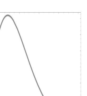
Figure 3: Dimensionless spectral power $\frac{I}{T^{3}}$ of a black body as a function of dimensionless frequency $Y\equiv\frac{\omega}{T}$ at T=10 K. The black (gray) curve depicts the modified (conventional) spectrum.

In Fig. 4 the low-frequency part of the spectrum, where the deviation from the conventional case is best visible, is indicated.

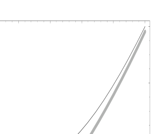
Figure 4: Zoom-in of the low-frequency part at T=10 K. The black (gray) curve depicts the modified (conventional) spectrum.

The deviation $\delta\rho\equiv\rho_{\mathrm{SU}(2)}-\rho_{\mathrm{U}(1)}$ of the energy density then is calculated as

$$\delta\rho=\int_{0}^{\infty}\mathrm{d}\omega\,I_{\mathrm{SU}(2)}-\int_{0}^{\infty}\mathrm{d}\omega\,I_{\mathrm{U}(1)}<0\,.$$ (4)

3 Dynamics of temperature evolution

In this section we derive the dynamic equations governing the cosmic evolution of temperature fluctuations. In a first step, we perform a match to the situation of a perfect fluid which enables us to interprete temperature as a scalar field subject to an adiabatic approximation. This situation is not unlike the one of a thermalized condensed matter system where the evolution of temperature inhomogeneities is described by a heat equation in which temperature plays the role of an scalar field under rotations. Subsequently, we allow for deviations from the adiabatic limit to obtain a dynamic temperature evolution. Finally, we derive the linearized evolution equation for temperature fluctuations sourced by the anomaly in the black-body spectrum [8, 9]. This evolution leads to the situation as sketched in Fig. 5. Namely, an initial inhomogeneity, maximal within a sufficiently large spatial domain within its horizon, provides for a local gradient of temperature which, under the influence of the black-body anomaly (scattering of photons off of monopoles and antimonopoles) is driven to even larger gradients as the Universe cools down. Thus a profile develops with maximal growth rate in the vicinity of redshift $z=1$. As a consequence, an observer situated a certain distance away from the center of the initial homgeneity measures a dipole distribution of CMB temperature within his own horizon. For a terrestial analogue imagine a volcano which after erruption 2D isotropically belches lava across the edge of its crater. A hypothetic observer situated at a lower point on the volcano’s slope preceives a downhill-directed (2D radial) lava flow.

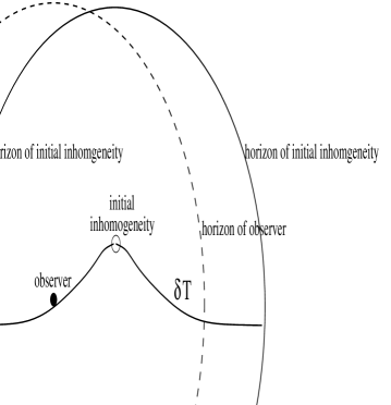
Figure 5: The situation relevant for the dynamic contribution to the CMB dipole after the black-body anomaly has evolved an initial inhomogeneity, for a detailed explanation see text.

3.1 Temperature as a scalar field

Let us now investigate to what extent it is possible to regard temperature as a scalar field. We start be considering the energy-momentum tensor $T_{\mu\nu}$ of a perfect fluid whose energy density $\rho$ and pressure $p$ are functions of temperature $T$:

$$T_{\mu\nu}=(\rho+p)u_{\mu}u_{\nu}-pg_{\mu\nu}\,,$$ (5)

where $u_{\mu}$ is the four-velocity of a fluid segment or the local rest frame of the heat bath, and the signature of the metric tensor $g_{\mu\nu}$ is $(1,-1,-1,-1)$. We now seek an action which produces the right-hand side of Eq. (5) upon using the definition for gravitationally consistent energy-momentum:

$$T_{\mu\nu}=\frac{1}{\sqrt{-g}}\frac{\delta\mathcal{L}}{\delta g^{\mu\nu}}\,.$$ (6)

Here $\mathcal{L}$ is s scalar action density and $\mbox{det}\,g_{\mu\nu}\equiv g$. For a static, perfect fluid the only two nonscalar covariants available to construct this scalar density are $u_{\mu}$, the local four-velocity of the fluid, and $g_{\mu\nu}$. Thus we make the ansatz

$$\mathcal{L}=\sqrt{-g}\left(\alpha\,u_{\mu}u_{\nu}g^{\mu\nu}+\beta\right)$$ (7)

with scalar parameters $\alpha$ and $\beta$ to be determined such that the perfect-fluid form in Eq. (5) emerges when employing Eq. (6). Notice that in varying the action density in Eq. (7) after $g^{\mu\nu}$ the four velocity $u_{\mu}$ is kept fixed. The connection between $u_{\mu}$ and $g^{\mu\nu}$ is made subsequently by virtue of Einstein’s equations.

Comparing the coefficients in front of the two independent tensor structures in Eq. (5) yields:

$$\alpha=\rho+p\,,\ \ \ \ \ \ \ \ \ \ \beta=-\rho-3p\,.$$ (8)

Thus the Lagrangian density in Eq. (7) becomes

$$\mathcal{L}=\sqrt{-g}\left((\rho+p)\underbrace{u_{\mu}u_{\nu}g^{\mu\nu}}_{=1}-\rho-3p\right)=-2\sqrt{-g}\,p\,.$$ (9)

Specializing to a conventional photon gas with equation of state $\rho=3p$, we have

$$\mathcal{L}=-\frac{2}{3}\sqrt{-g}\,\rho\,.$$ (10)

Since $\rho\propto T^{4}$ it follows that temperature itself acquires the status of a scalar field within the static, perfect-fluid situation.

3.2 Temperature fluctuations

The Lagrangian density in Eq. (10) represents a potential for the scalar field $T$. We would like to go beyond this adiabatic approximation by allowing for the contributions of derivatives in $\delta T$:

$$T=\bar{T}(t)+\delta T(t,{\bf x})\,.$$ (11)

Since $\bar{T}(t)$ is a homogeneous, scalar field corresponding to the limit of noninteracting photons the deviation from this limit $\delta T(t,{\bf x})$ is also associated with a scalar field. The deviation $\delta\rho$ of the energy density due to the black-body anomaly, see Sec. 2, induces the fluctuation $\delta T$ about the mean temperature $\bar{T}$. The latter is redshifted by the evolution of the cosmological background. We consider the conventional black-body part $\bar{\rho}({\bar{T}})\equiv\rho_{\mathrm{U}(1)}=\frac{\pi^{2}}{45}\,{\bar{T}}^{4}$ as a fluid which, among other contributions (cold dark matter and dark energy), sources spatially flat Friedmann-Robertson-Walker (background) cosmology:

$$\mathrm{d}s^{2}=g_{\mu\nu}\,\mathrm{d}x^{\mu}\mathrm{d}x^{\nu}\equiv\mathrm{d}t^{2}-a^{2}(t)\mathrm{d}{\bf x}^{2}\,,$$ (12)

where $a(t)$ denotes the scale factor.

To make the action a scalar the usual factor of $\sqrt{-g}$ in the action density is expressed in terms of $\bar{T}$ and $\bar{T_{0}}\equiv T_{c}$ by virtue of the identity

$$\frac{a(t)}{a_{0}}=\frac{\bar{T}_{0}}{\bar{T}}\ \ \ \ \Rightarrow\ \ \ \ \sqrt{-g}=\left(\frac{\bar{T}_{0}}{\bar{T}}\right)^{3}\,,\ \ \ (a_{0}\equiv 1)\,.$$ (13)

In Eq. (13) and in the remainder of the article a subscript ‘0’ refers to today’s value of the corresponding quantity. Recall that our present Universe necessarily is very close to $T_{c}=2.73\,$K to avoid a contradiction with astrophysical observation: There is no screening effect in the propagation of photons above the CMB ground state emitted by astrophysical sources situated astrophysically (not cosmologically!) far away.

Leaving the limit of noninteracting photons, the action for $\delta T(t,{\bf x})$ is a series involving scalar combinations of arbitrarily high powers of derivatives $\partial_{\mu}$. The mass scale $l^{-1}$, which determines the relevance of the $n$th power of $\partial_{\mu}$ in this expansion, is, however, determined by the mass of a screened monopole: $l^{-1}\sim\frac{4\pi}{e}\pi T$ where $e=\sqrt{8}\pi$ away from the deconfining-preconfining phase boundary, recall that there is a (logarithmic) divergence in $e$ at $T_{c}$ [4, 21]. Thus $l^{-1}$ is comparable to temperature itself. Derivatives, however, measure deviations of temperature on cosmological scales and thus, for counting purposes, the $n$th power of a derivative ($n$ even) can be replaced by the $n$th power of the Hubble parameter $H$. For the regime of redshift we are interested in ($z\leq 40$ or so) the parameter $\frac{H}{T}$ is extremely small and thus a truncation of the expansion of the action into powers of derivatives at $n=2$ is justified. There is not yet precise theoretical prescription on how to fix the coefficient in front of this kinetic term for $\delta T$ although linear-response analysis should be applicable. Being pragmatic, we allow here for a dimensionless coefficient $k$ whose numerical value needs to be determined observationally. Using Eq. (13) we have:

$$\sqrt{-g}\,\mathcal{L}_{\tiny\mbox{CMB}}=\left(\frac{\bar{T}_{0}}{\bar{T}}\right)^{3}\left(k\,\partial_{\mu}\delta T\partial^{\mu}\delta T-\delta\rho(T)\right)\,.$$ (14)

Let us now define a function $\hat{\rho}(T,T_{0})$ as

$$\delta\rho=T_{0}^{2}\,\hat{\rho}\,.$$ (15)

Varying the action associated with Eq. (14) w.r.t. $\delta T$ and linearizing the resulting equation of motion then yields:

$$\partial_{\tilde{\mu}}\partial^{\tilde{\mu}}\delta T-\frac{3}{\bar{T}}\,\partial_{\tau}\bar{T}\,\partial_{\tau}\delta T+\frac{\bar{T}_{0}^{2}}{kH_{0}^{2}}\left[\frac{1}{2}\,\left.\frac{\mathrm{d}^{2}\hat{\rho}}{\mathrm{d}T^{2}}\right|_{T=\bar{T}}\,\delta T+\frac{1}{2}\,\left.\frac{\mathrm{d}\hat{\rho}}{\mathrm{d}T}\right|_{T=\bar{T}}\right]=0\,.$$ (16)

In Eq. (16) we have performed the coordinate transformation

$$\tilde{x}_{0}\equiv\tau=H_{0}\,t\,,\ \ \ \ \ \ \ \ \ \tilde{x}_{i}=\frac{\mathrm{d}a}{\mathrm{d}t}\,x_{i}\,,\ \ \ \ \ (i=1,2,3)\,.$$ (17)

Notice the extremely large factor $(\bar{T}_{0}/H_{0})^{2}\sim 10^{60}$ in front of the square brackets in Eq. (16). This factor arises because we chose to measure time $\tau$ in units of the age of the Universe, distances from the origin $\tilde{x}_{i}$ in units of the actual horizon size $H^{-1}=a/\frac{\mathrm{d}a}{\mathrm{d}t}$ (as long as $|\tilde{x}_{i}|$ is sufficiently smaller than unity), and temperature in units of $\bar{T}_{0}=2.35\times 10^{-4}\,$eV.

Assuming spherical symmetry for the fluctuation $\delta T$, which is relevant for an analysis of the cosmic dipole, see Sec. 4.1, Eq. (16) reads:

$$0 = \partial_{\tau}\partial_{\tau}\delta T-\left(\frac{\mathrm{d}a}{\mathrm{d}\tau}\right)^{2}\,\left[\partial_{\sigma}\partial_{\sigma}\delta T+\frac{2}{\sigma}\,\partial_{\sigma}\delta T\right]-\frac{3}{\bar{T}}\,\partial_{\tau}\bar{T}\,\partial_{\tau}\delta T+$$ (18)

$$\frac{\bar{T}_{0}^{2}}{kH_{0}^{2}}\left[\frac{1}{2}\,\left.\frac{\mathrm{d}^{2}\hat{\rho}}{\mathrm{d}T^{2}}\right|_{T=\bar{T}}\,\delta T+\frac{1}{2}\,\left.\frac{\mathrm{d}\hat{\rho}}{\mathrm{d}T}\right|_{T=\bar{T}}\right]\,.$$

In Eq. (18) we have introduced $\sigma\equiv\sqrt{\tilde{x}_{1}^{2}+\tilde{x}_{2}^{2}+\tilde{x}_{3}^{2}}$. This equation is a two-dimensional wave equation with additional terms arising on one hand due to the time-dependence of the cosmological background ($-\frac{3}{\bar{T}}\,\partial_{\tau}\bar{T}\,\partial_{\tau}\delta T$) and on the other hand due to the presence of the black-body anomaly: The term $\frac{1}{2}\frac{\bar{T}_{0}^{2}}{kH_{0}^{2}}\left.\frac{\mathrm{d}^{2}\hat{\rho}}{\mathrm{d}T^{2}}\right|_{T=\bar{T}}\,\delta T$ will be referred to as ‘restoring term’, and the term $\frac{1}{2}\,\frac{\bar{T}_{0}^{2}}{kH_{0}^{2}}\left.\frac{\mathrm{d}\hat{\rho}}{\mathrm{d}T}\right|_{T=\bar{T}}$ will be referred to as ‘source term’ in the following.

3.3 Background evolution

Here we would like to provide some information about the simple $\Lambda$CDM model for the background cosmology which fits the data best [2, 16, 17, 18]. We assume a spatially flat Universe subject to the following Friedmann equation

$$\left(\frac{\dot{a}}{a}\right)^{2}={H_{0}}^{2}\left(\frac{\Omega_{m}}{a^{3}}+\Omega_{\Lambda}\right)$$ (19)

where $\Omega_{m}=0.24$ and $\Omega_{\Lambda}=1-\Omega_{m}=0.76$ (fit obtained from WMAP three-year data [19]) are the cold dark-matter and the dark-energy density, respectively, both in units of the critical density. $H_{0}$ is today’s value of the Hubble parameter, and $\dot{a}\equiv\frac{\mathrm{d}a}{\mathrm{d}t}$. The solution to Eq. (19) is

$$a(t)=\left(\frac{\Omega_{m}}{\Omega_{\Lambda}}\right)^{1/3}\left[\sinh{\frac{3\,\sqrt{\Omega_{\Lambda}}}{2}\,H_{0}t}\right]^{2/3}\,,$$ (20)

where $H_{0}$ is connected to $t_{0}$ (present age of the Universe) as

$$H_{0}t_{0}=\frac{1}{3\sqrt{1-\Omega_{m}}}\ln{\frac{2-\Omega_{m}+2\sqrt{1-\Omega_{m}}}{\Omega_{m}}}\,,$$ (21)

and we use the convention that $a_{0}\equiv a(t_{0})=1$. The mean temperature $\bar{T}$ then follows from Eqs. (13) and (20). As a reminder we give the relation between scale factor $a$ and redshift $z$ since we present our results as functions of $z$:

$$a(z)=\frac{1}{1+z}\,,\ \ \ \ \ \ (a_{0}\equiv a(z=0)=1)\,.$$ (22)

4 Numerical analysis

4.1 Principle remarks and boundary conditions

To identify a dynamic component in the CMB dipole, which dominates the higher multipoles by two orders of magnitude, the associated solution to Eq. (16) must locally exhibit a singled-out direction. This implies spherical symmetry about the center of an initial inhomogeneity which, by the source term in Eq. (18), induces the built-up of the spatially extended, spherically symmetric profile $\delta T$. Notice that a superposition of solutions obtained for several such isolated inhomogeneities is not a solution of Eq. (16) due to the presence of the spatially homogeneous source term. Notice also that such an initial situation would evolve to populate higher multipoles of comparable strength as the dipole. This, however, is rules out by observation. We conclude that in describing a dynamic component to the CMB dipole spherical symmetry of the fluctuation $\delta T$ is imperative within the horizon of the center of the inducing, initial inhomogeneity. Then almost each observer perceives a modulus of the dynamic CMB-dipole component which is nearly independent of his position. That is, the mean radial gradient approximately serves to define a singled-out direction except at the center of the (as we shall see) bump-like $\delta T$. This exception, however, occurs with vanishing likelihood geometrically, see Fig. 5.

The modulus of the dynamic component ${\bf D}_{\tiny\mbox{dyn}}$, as it would be perceived by an observer situated a radial distance $\sigma_{0}$ away from the center of the bump, then is defined as follows

$$|{\bf D}_{\tiny\mbox{dyn}}|\equiv\int^{1}_{\sigma_{0}}d\xi\,\delta T(z=0,\xi)-\int^{\sigma_{0}}_{\sigma_{0}-1}d\xi\,\delta T(z=0,\xi)\,.$$ (23)

The upper limit in the first integral arises from the fact that for $\sigma\geq 1$ the nonexistence of a causal connection to the center of the bump forbids the built-up of a profile. The definition in Eq. (23) states that $|{\bf D}_{\tiny\mbox{dyn}}|$ is roughly given by the mean gradient of $\delta T$.

Now the coefficient $k$ in Eq. (18) is determined such that the mean gradient in $\delta T(z=0,\sigma)$ coincides with the dynamic component in the CMB dipole. The latter is attributed to the following discrepancy: On one hand, the velocity of the Local Group ${\bf v}_{\tiny\mbox{LG,dir}}$ can be determined directly by estimating the gravitational impact on it by all those galaxies contained in successively enlarged concentric, spherical shells and by observing saturation for $zc\geq 6000\,$km s^-1 [22]. Here $c$ is the velocity of light. It is found that $|{\bf v}_{\tiny\mbox{LG,dir}}|\sim 400\,$km s^-1 with errors typically being $\sim 50\,$km s^-1 [22]. On the other hand, the conventional understanding of the CMB dipole as a purely kinematic effect [23], which implies a velocity of the solar system of ${\bf v}_{\tiny\mbox{SS}}=(369\pm 2)\,$km s^-1 [24], plus the known relative velocity ${\bf v}_{\tiny\mbox{LG-SS}}$ between the solar system and the Local Group allows to deduce a velocity of the Local Group of $|{\bf v}_{\tiny\mbox{LG,dedu}}|\sim 619\,$ km s^-1 [26]. In this way the angle $\delta\equiv\angle{\bf v}_{\tiny\mbox{LG,dedu}},{\bf v}_{\tiny\mbox{LG,dir}}$ is extracted as $\delta=(13\pm 7)^{o}$ [22]. As a consequence, a deficit velocity ${\bf v}_{\tiny\mbox{dyn}}={\bf v}_{\tiny\mbox{LG,dedu}}-{\bf v}_{\tiny\mbox{LG,dir}}$ is generated which must have a dynamic origin.

Let us explain this in more detail: On one hand, the velocity ${\bf v}_{\tiny\mbox{LG,dir}}$ generates a kinematic contribution to the CMB dipole, ${\bf D}_{\tiny\mbox{LG,kin}}$, whose amplitude $\Delta T\equiv\frac{1}{2}\,|{\bf D}_{\tiny\mbox{LG,kin}}|$ is calculable according to [23] as

$$\Delta T=\frac{|{\bf v}|}{c}\,\bar{T}_{0}+{\cal O}\left(\frac{{\bf v}^{2}}{c^{2}}\right)\,.$$ (24)

On the other hand, the CMB dipole ${\bf D}_{\tiny\mbox{SS}}$, as it is measured in the solar-system rest frame, is supplemented by a purely kinematic contribution ${\bf D}_{\tiny\mbox{LG-SS,kin}}$ resulting from the relative velocity ${\bf v}_{\tiny\mbox{LG-SS}}$ between the solar system and the Local Group. This yields the CMB dipole ${\bf D}_{\tiny\mbox{LG,true}}$ as it is perceived in the rest frame of the Local Group. Knowing ${\bf v}_{\tiny\mbox{LG,dedu}}$, we can compute ${\bf D}_{\tiny\mbox{LG,true}}$ by means of Eq. (24). Since

$${\bf D}_{\tiny\mbox{LG,true}}={\bf D}_{\tiny\mbox{LG,kin}}+{\bf D}_{\tiny\mbox{dyn}}$$ (25)

the dynamic contribution to the CMB dipole ${\bf D}_{\tiny\mbox{dyn}}$ follows. In Fig. 6 this situation is sketched.

Figure 6: Diagram relating observed and deduced quantities concerned with CMB-dipole physics.

Let us now discuss the boundary conditions which Eq. (18) needs to be supplemeted with. Eq. (18) is an inhomogeneous, linear, partial differential equation which can be solved using the numerical method of lines, see [27]. Four boundary conditions are required, two for the temporal and two for the spatial evolution. We assume the spatial distribution of the initial fluctuation at redshifts $z_{i}=5...30$ to be of Gaussian shape with its height chosen such that $\frac{\delta T(z_{i},\sigma=0)}{\bar{T}(z_{i})}=10^{-5}$ as is expected to be provided by primordial causes:

$$\delta T(z_{i},\sigma)=10^{-5}\,\bar{T}(z_{i})\,\mbox{e}^{-(\frac{\sigma}{w})^{2}}\,.$$ (26)

Here the subscript $i$ refers to ‘initial’. The width $w$ of the Gaussian in Eq. (26) will be varied to check for the robustness of the result against our ignorance concerning this boundary condition.

Initially, we assume the built-up of the fluctuation to be slow since the source term $\frac{1}{2}\left.\frac{\mathrm{d}\,\delta\rho}{\mathrm{d}T}\right|_{T=\bar{T}}$ in Eq. (18) driving this built-up is small for sufficiently large initial redshift $z_{i}$, see Fig. 7. That is, we prescribe

$$\partial_{\tau}\delta T(\tau,\sigma)\bigr{|}_{\tau=\tau_{i}}=0$$ (27)

and later check for the independence of the result on our choice of $z_{i}$. For a comparison of orders of magnitude between the two terms in Eq. (18) dependent on the black-body anomaly, the coefficient $\frac{1}{2}\left.\frac{\mathrm{d^{2}\delta\rho}}{\mathrm{d}T^{2}}\right|_{T=\bar{T}}$ of $\delta T$ in the ‘restoring term’ is depicted as a function of $z$ in Fig. 8, and in Fig. 7 the corresponding plot for the ‘source term’ is shown. Since our simulations yield $\delta T<10^{-2}\,$K we conclude that the ‘source term’ strongly dominates the ‘restoring term’.

Figure 7: The ‘source term’ $\frac{1}{2}\left.\frac{\mathrm{d}\,\delta\rho}{\mathrm{d}T}\right|_{T=\bar{T}}$ in Eq. (18) as a function of redshift $z$.

Figure 8: The coefficient $\frac{1}{2}\left.\frac{\mathrm{d^{2}\delta\rho}}{\mathrm{d}T^{2}}\right|_{T=\bar{T}}$ in the ‘restoring term’ of Eq. (18) as a function of redshift $z$.

As a function of $\sigma$ the fluctuation $\delta T$, being either weakened or enforced during the evolution, remains extremal at $\sigma=0$ where the initial inhomogeneity (a seed for $\delta T$) was located. So it should satisfy

$$\partial_{\sigma}\delta T(\tau,\sigma)\bigr{|}_{\sigma=0}=0\,.$$ (28)

Finally, $\delta T$ is zero for $\sigma\geq 1$ (horizon) and for all times. Otherwise, the built-up of $\delta T$ would be noncausal:

$$\delta T(\tau,\sigma\geq 1)=0\,.$$ (29)

In order to be consistent with the b.c. in Eq. (26), we approximate the b.c. of Eq. (29) by simply prescribing the value of the profile $\delta T$ at $z_{i}=0$ and $\sigma=1$ for all $z$. This is in good agreement with Eq. (29) if $w\ll 1$.

4.2 Values for $k$ and higher multipoles

The coefficient $k$ in Eq. (18) is chosen such that half of the mean gradient of the profile $\delta T$ at $z=0$ equals the observationally inferred amplitude $\Delta T$ for the dynamic contribution $|{\bf D}_{\tiny\mbox{dyn}}|$. We impose one observationally suggested set ($A$) and one set with a fictitiously large angle $\delta$ and an upper-limit value for $|{\bf v}_{\tiny\mbox{LG,dir}}|$ ($B$) (taking $|{\bf v}_{\tiny\mbox{LG,dedu}}|\sim 627\,$ km s^-1) as

$$(A): \ |{\bf v}_{\tiny\mbox{LG,dir}}|=400\,\mbox{km\,s}^{-1}\,,\ \ \ \delta=13^{o}\ \ \ \Rightarrow$$

$$\ |{\bf v}_{\tiny\mbox{dyn}}|=253.74\,\mbox{km\,s}^{-1}\,,\ \ \ |{\bf D}_{\tiny\mbox{dyn}}|=2.311\,\mbox{mK}\ \ \ \Rightarrow\ \ \ k=0.01868\,\bar{T}_{0}^{2}/H_{0}^{2}\,;$$

$$(B): \ |{\bf v}_{\tiny\mbox{LG,dir}}|=450\,\mbox{km\,s}^{-1}\,,\ \ \ \delta=30^{o}\ \ \ \Rightarrow$$

$$\ |{\bf v}_{\tiny\mbox{dyn}}|=327.00\,\mbox{km\,s}^{-1}\,,\ \ \ |{\bf D}_{\tiny\mbox{dyn}}|=2.978\,\mbox{mK}\ \ \ \Rightarrow\ \ \ k=0.01449,\bar{T}_{0}^{2}/H_{0}^{2}\,.$$

In writing the two values for $k$ in Eq. (4.2) we have anticipated some results of Sec. 4.3. Namely, our simulations indicate that the mean gradient of the profile $\delta T$ at $z=0$ does not depend on $z_{i}$ for $5\leq z_{i}\leq 30$, does not depend on the width $w$ in Eq. (26), and does not depend on the height for

$$0\leq\delta T(z=0,\sigma=0)\leq 10^{-5}\,\bar{T}(z=0)\,.$$ (31)

The mean gradient does, however, depend roughly linearily on the strength of the source term in Eq. (18) thus generating a definite value for $k$.

On one hand, a virtue of the model is to accommodate the possiblity for ${\bf D}_{\tiny\mbox{dyn}}$, the latter serving to fix the value of the coefficient $k$. On the other hand, once $k$ is fixed by this observational input a calculation of the dipole-subtracted large-angle correlation function (with a slight abuse of notation)

$$C(\theta)\equiv\left\langle\delta T_{\tiny\mbox{dyn},l\geq 2}(\hat{e}_{1}),\delta T_{\tiny\mbox{dyn},l\geq 2}(\hat{e}_{2})\right\rangle\,,\ \ \ \ \ (\theta\equiv\angle\hat{e}_{1},\hat{e}_{2})\,,$$ (32)

is enabled by virtue of Eq. (16). Namely, by subtracting Eq. (18) (dynamic contribution $\delta T_{\tiny\mbox{dyn},l=1}$ to the dipole) from Eq. (16) (general fluctuation $\delta T_{\tiny\mbox{dyn}}$, not imposing spherical symmetry) we arrive at

$$\partial_{\tilde{\mu}}\partial_{\tilde{\mu}}\delta T_{\tiny\mbox{dyn},l\geq 2}-\frac{3}{\bar{T}}\,\partial_{\tau}\bar{T}\,\partial_{\tau}\delta T_{\tiny\mbox{dyn},l\geq 2}+\frac{1}{2}\,\frac{\bar{T}_{0}^{2}}{kH_{0}^{2}}\,\left.\frac{\mathrm{d}^{2}\hat{\rho}}{\mathrm{d}T^{2}}\right|_{T=\bar{T}}\,\delta T_{\tiny\mbox{dyn},l\geq 2}=0\,,$$ (33)

where $\delta T_{\tiny\mbox{dyn},l\geq 2}\equiv\delta T_{\tiny\mbox{dyn}}-\delta T_{\tiny\mbox{dyn},l=1}$. That is, dipole-subtracted fluctuations obey a wave equation with a cosmological damping term and a ‘restoring term’ (second derivative of the black-body anomaly $\delta\rho$ times $\delta T_{\tiny\mbox{dyn},l\geq 2}$). Actually, Eq. (33) is an approximation assuming that the built-up of the dynamic contribution to the dipole consumes the entire source term and that no influence of this term on the higher multipoles takes place. To check whether this, indeed, is the case the solution to Eq. (16) would have to be projected onto its multipoles, and the dipole component would have to be compared with the solution to Eq. (18). In any case, Cartesian two-point correlations of $\delta T_{\tiny\mbox{dyn},l\geq 2}$ at $z=0$, which are required to postdict $C(\theta)$, can be computed by an average with primordially provided initial conditions of the product

$$\delta T_{\tiny\mbox{dyn},l\geq 2}(z=0,{\bf\tilde{x}_{1}})\,\delta T_{\tiny\mbox{dyn},l\geq 2}(z=0,{\bf\tilde{x}_{2}})\,,$$ (34)

where $\delta T_{\tiny\mbox{dyn},l\geq 2}$ either is a solution to Eq. (33) or the according projection onto the multipole $l\geq 2$ of a solution to Eq. (16) (classical approximation, see [28, 29]). The correlation function $C(\theta)$ then follows as

$$C(\theta)=\int_{0}^{1}d|{\bf\tilde{x}_{1}}|\,\int_{0}^{1}d|{\bf\tilde{x}_{2}}|\,\left\langle\delta T_{\tiny\mbox{dyn},l\geq 2}(z=0,|{\bf\tilde{x}_{1}}|\hat{e}_{1})\,\delta T_{\tiny\mbox{dyn},l\geq 2}(z=0,|{\bf\tilde{x}_{2}}|\hat{e}_{2})\right\rangle\,,$$ (35)

and one can check the usual assumption made about statistical isotropy by varying $\hat{e}_{1},\hat{e}_{2}$ while keeping $\theta$ fixed. This analysis is reserved for future work.

4.3 Results of numerical calculation

Here we present the results of our numerical calculation. Fig. 9 shows the fluctuation $\delta T$ for $\sigma=0.5;0.05$ as a function of redshift $z$ with a width of the initial Gaussian assumed as $w=10^{-2}$.

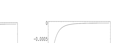
Figure 9: $\frac{\delta T}{\bar{T}}$ at two distances $\sigma=0.5$ (black curve) and $\sigma=0.05$ (gray curve) as a function of $z$ setting $z_{i}=20$. The left (right) panel corresponds to $k=0.01868\,\bar{T}_{0}^{2}/H_{0}^{2}$ ($k=0.01449\,\bar{T}_{0}^{2}/H_{0}^{2}$). A width $w=10^{-2}$ of the initial Gaussian was assumed.

Obviously, the major contribution to $\frac{\delta T}{\bar{T}}$ is generated within $0\leq z\leq 1$ corresponding to a temperature range $T_{0}=2.73\,\mbox{K}\leq T\leq 8.1\,$K. This is expected from the discussion in [8, 9]. We have checked that, switching off the source term in Eq. (18) and keeping all other conditions the same, the initial profile oscillates in a strongly damped way. This is consistent with our finding that the evolution in $z$ as described by Eq. (18) possesses an attractor which is determined by this source term, see below.

In Figs. 10 and 11 we show $\frac{\delta T}{\bar{T}}$ as a function of $\sigma$ at $z=0$ and $z=1$ when varying the shape of the initial profile at $z_{i}=20$. Our results are practically independent of these initial conditions. Again, it is seen that the major contribution to the profile at $z=0$ is being built up for $0\leq z\leq 1$.

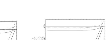
Figure 10: $\frac{\delta T}{\bar{T}}$ for two values of $z$ as a function of $\sigma$: $z=0$ (black curves: solid line contains the cases $w=10^{-1}$ and $w=10^{-4}$, there is practically no difference; dashed curve corresponds to $w=\infty$) and $z=1$ (gray curves: same as for black curves). The initial redshift is $z_{i}=20$, the left (right) panel corresponds to $k=0.01868\,\bar{T}_{0}^{2}/H_{0}^{2}$ ($k=0.01449\,\bar{T}_{0}^{2}/H_{0}^{2}$).

Figure 11: $\frac{\delta T}{\bar{T}}$ for two values of $z$ as a function of $\sigma$: $z=0$ (two lower curves: initial Gaussian distribution with width $w=10^{-2}$ (black) and vanishing initial distribution (gray); $z=1$ (two upper curves: initial Gaussian distribution with width $w=10^{-2}$ (dark gray) and vanishing initial distribution (light gray);). The initial redshift is $z_{i}=20$, the left (right) panel corresponds to $k=0.01868\,\bar{T}_{0}^{2}/H_{0}^{2}$ ($k=0.01449\,\bar{T}_{0}^{2}/H_{0}^{2}$).

Next, we investigate the dependence of the distribution on changes in $z_{i}$. Fig. 12 shows $\frac{\delta T}{\bar{T}}$ as a function of $\sigma$ at $z=0$ and $z=1$ for $z_{i}=5$, $z_{i}=20$, and $z_{i}=40$. Obviously, there is hardly any dependence on $z_{i}$.

Figure 12: $\frac{\delta T}{\bar{T}}$ as a function of $\sigma$ for a width of the initial Gaussian distribution of $w=10^{-2}$ and for $z=0$ (lower curves) and $z=1$ (upper curves). The initial redshifts are chosen as $z_{i}=5$, $z_{i}=20$, and $z_{i}=40$. The left (right) panel corresponds to $k=0.01868\,\bar{T}_{0}^{2}/H_{0}^{2}$ ($k=0.01449\,\bar{T}_{0}^{2}/H_{0}^{2}$).

The plots in Fig. 10 indicate a discontinuity at $\sigma=0$. As demonstrated by Fig. 13, this is an artefact of the finite lattice constant when solving Eq. (18).

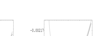
Figure 13: $\frac{\delta T}{\bar{T}}$ for $z=0$ as a function of $\sigma$ for varying lattice constants (black curve: grid with 1000 points; gray curve: grid with 100 points). The width of the initial Gaussian distribution is $w=10^{-2}$, the initial redshift is $z_{i}=20$, and the left (right) panel corresponds to $k=0.01868\,\bar{T}_{0}^{2}/H_{0}^{2}$ ($k=0.01449\,\bar{T}_{0}^{2}/H_{0}^{2}$).

5 Conclusion and Outlook

In the present article we have discussed a model for the temperature-temperature correlation in the cosmic microwave background (CMB) at large angular separation. The key idea is to relate the discrepancy between the observed and the CMB-inferred velocity of the Local Group to a dynamic component in the CMB dipole.

The origin of this dynamic component is tied to an anomaly in black-body spectra as it is predicted by deconfining SU(2) Yang-Mills thermodynamics when postulating that $SU(2)_{\tiny\mbox{CMB}}\stackrel{{\scriptstyle\tiny\mbox{today}}}{{=}}U(1)_{Y}$, see [4, 5, 6, 8, 9]. The black-body anomaly, in turn, is computed in the effective theory for deconfining SU(2) Yang-Mills thermodynamics [4] in terms of a one-loop diagram fixing the (on-shell) polarization tensor of the massless mode [9]. As it seems, the polarization tensor for the massless mode is one-loop exact [10]. What is described by the polarization tensor in the effective theory is, on the microscopic level, the effect on the thermal spectral intensity of photon scattering off of electrically charged monopoles. The rate of change of the modified as compared to the conventional black-body spectrum in dependence of mean temperature $\bar{T}$ is maximal at $\bar{T}\sim 2\times T_{c}\sim 2\times 2,73\,$K or redshift $z\sim 1$. Primordial temperature inhomogeneities are enforced or weakened on the scale of $\frac{\delta T}{\bar{T}}\sim 10^{-2}$ in this regime leading to the emergence of a spherical profile maximal at a center and vanishing for distances larger than horizon scale away from this center. The radial gradient of this profile is interpreted as a dynamic contribution to the dipole in the CMB temperature anisotropy thus accomodating the discrepancy between the directly observed and the inferred (by virtue of the realtivistic Doppler effect) velocity of the the Local Group w.r.t. the CMB rest frame. The rapid built-up of the spherical profile would then be responsible for ‘inflating away’ primordial large-scale anisotropies thus explaining the the missing power observed by WMAP [2]: For a 2D analogue imagine a fluctuating rubber scarf enframed by a spherical boundary. Large-scale fluctuations are smoothened out by the process of pinching the scarf centrally and quickly pulling it out of the plane into a conical profile. In addition, the resulting and suppressed large-scale fluctuations would necessarily be correlated due to the common cause for their suppression [30].

Our numerical simulations of the spherically symmetric case indicate that the results are very robust against changes in the initial conditions. The main contribution to the built-up of the temperature profile arises for $z\sim 1$. Assuming an adiabatically slow cooling of the CMB driven by a $\Lambda$CDM background cosmology, this corresponds to the regime in temperature $\bar{T}$ where $\frac{\delta T}{\bar{T}}$ changes most rapidly, see Fig. 2.

To substantiate the here-developed scenario further a dedicated simulation of Eq. (16) will be needed. Our future work thus will focus on the computation of dipole-subtracted large-angle correlations based on the model proposed here.

References

- [1] E. Zavattini et al., Phys. Rev. Lett. 96, 110406 (2006).
-
[2]
A. Kogut et al., Astrophys. J. Suppl. 148, 161 (2003).
D. N. Spergel et al., Astrophys. J. Suppl. 148, 175 (2003).
D. N. Spergel et al., astro-ph/0603449.
L. Page et al., astro-ph/0603450.
G. Hinshaw et al., astro-ph/0603451.
N. Jarosik et al., astro-ph/0603452. - [3] L. B. G. Knee and C. M. Brunt, Nature 412, 308 (2001).
-
[4]
R. Hofmann, Int. J. Mod. Phys. A20, 4123 (2005), Erratum-ibid A21, 6515 (2006).
R. Hofmann, Mod. Phys. Lett. A21, 999 (2006), Erratum-ibid. A 21, 3049 (2006). - [5] R. Hofmann, PoS JHW2005, 021 (2006) [hep-ph/0508176].
- [6] F. Giacosa and R. Hofmann, Eur. Phys. J. C 50, 635 (2007).
- [7] D. Diakonov, N. Gromov, V. Petrov, S. Slizovskiy, Phys. Rev. D 70, 036003 (2004).
- [8] M. Schwarz, R. Hofmann, and F. Giacosa, JHEP 0702, 091 (2007).
- [9] M. Schwarz, R. Hofmann, and F. Giacosa, Int. J. Mod. Phys. A22, 1213 (2007).
- [10] D. Kaviani and R. Hofmann, Mod. Phys. Lett. A 22, 2343 (2007).
- [11] R. Hofmann, hep-th/0609033.
- [12] M. Szopa, R. Hofmann, F. Giacosa, and M. Schwarz, arXiv:0707.3020 [hep-ph]
-
[13]
C. P. Korthals Altes (Marseille, CPT),
in *Minneapolis 2006, Continuous advances in QCD* 266-272
[hep-ph/0607154].
C. Korthals-Altes and A. Kovner, Phys. Rev. D 62, 096008 (2000) [hep-ph/0004052].
C. Korthals-Altes, hep-ph/0406138. - [14] F. Giacosa and R. Hofmann, Phys. Rev. D 76, 085022 (2007).
- [15] R. Hofmann, arXiv:0710.0962 [hep-th].
- [16] A. G. Riess et al., Astron. J. 116, 1009 (1998).
- [17] S. Perlmutter et al., Astrophys. J. 483, 565 (1998).
- [18] B. P. Schmidt et al., Astrophys. J. 507, 46 (1998).
- [19] D. N. Spergel et al., astro-ph/0603449.
-
[20]
M. F. Atiyah and N. J. Hitchin, Phil. Trans. Roy. Soc. Lond. A315, 459 (1985).
M. F. Atiyah and N. J. Hitchin, Phys. Lett. A107, 21 (1985). - [21] F. Giacosa and R. Hofmann, hep-th/0703127.
-
[22]
P. Erdogdu et al., Mon. Not. Roy. Astron. Soc.373, 45 (2006) [astro-ph/0610005].
P. Erdogdu et al., talk given at 41st Rencontres de Moriond, Workshop on Cosmology: Contents and Structures of the Universe, La Thuile, Italy, 18-25 Mar 2006 [astro-ph/0605343]. - [23] P. J. Peebles and D. T. Wilkinson, Phys. Rev.17, 2168 (1968).
- [24] G. Hinshaw et al., astro-ph/0603451.
- [25] Review of Particle Physics, Particle Data Group, p. 98 (2006).
- [26] A. Kogut et al., Astrophys. J. 419, 1 (1993).
- [27] W. E. Schiesser, Computational mathematics in Engineering and Applied Science: ODEs, DAEs and PDEs, CRC Press. (1994).
-
[28]
S. Yu. Khlebnikov and I. I. Tkachev, Phys. Rev. Lett. 77, 219 (1996).
S. Khlebnikov and I. I. Tkachev, Phys. Rev. Lett. 79, 1607 (1997). - [29] T. Prokopec and T. G. Roos, Phys. Rev. D55, 3768 (1997).
- [30] C. J. Copi, D. Huterer, D. J. Schwarz, and G. D. Starkman, Phys. Rev. D75, 023507 (2007).