The large degeneracy of excited hadrons and quark models

Abstract

The pattern of a large approximate degeneracy of the excited hadron spectra (larger than the chiral restoration degeneracy) is present in the recent experimental report of Bugg. Here we try to model this degeneracy with state of the art quark models. We review how the Coulomb Gauge chiral invariant and confining Bethe-Salpeter equation simplifies in the case of very excited quark-antiquark mesons, including angular or radial excitations, to a Salpeter equation with an ultrarelativistic kinetic energy with the spin-independent part of the potential. The resulting meson spectrum is solved, and the excited chiral restoration is recovered, for all mesons with $J>0$. Applying the ultrarelativistic simplification to a linear equal-time potential, linear Regge trajectories are obtained, for both angular and radial excitations. The spectrum is also compared with the semi-classical Bohr-Sommerfeld quantization relation. However the excited angular and radial spectra do not coincide exactly. We then search, with the classical Bertrand theorem, for central potentials producing always classical closed orbits with the ultrarelativistic kinetic energy. We find that no such potential exists, and this implies that no exact larger degeneracy can be obtained in our equal-time framework, with a single principal quantum number comparable to the non-relativistic Coulomb or harmonic oscillator potentials. Nevertheless we find plausible that the large experimental approximate degeneracy will be modelled in the future by quark models beyond the present state of the art.

I Introduction

In the recent report of Bugg Bugg:2004xu ; Afonin:2006vi ; Glozman:2007ek ; fig1afon a large degeneracy emerges from the spectra of the angularly and radially excited resonances produced in $p\bar{p}$ annihilation by the Crystal Ball collaboration at LEAR in CERN Aker:1992ny . This degeneracy may be the third remarkable pattern of the excited spectra of hadronic resonances.

A long time ago, Chew an Fautschi remarked the existence of linear Regge trajectories Chew for angularly excited mesons, and baryons Fiore:2004xb ; Yao:2006px . A similar linear aligning of excited resonances was also reported for radial excitations Anisovich:2001pn .

Recently, Glozman et al. Glozman:2007ek ; Wagenbrunn:2007ie ; Glozman have been systematically researching the degeneracy of chiral partners in excited resonances, both in models and in lattice QCD. Le Yaouanc et al. Yaouanc and PB et al. Bicudo_thesis ; Bicudo_hvlt developed a model of spontaneous symmetry breaking. Viewed retrospectively, this already included the degeneracy of chiral partners in the limit of high radial or angular excitations Malheiro , both in light-light and in heavy-light hadrons. This earlier work was based on the Bogoliubov transformation and used the Coulomb gauge or the local coordinate gauge QCD truncations. Here the formalism will be extended to include spin-dependent interactions explicitly.

The recent data on highly excited mesons, observed by LEAR at CERN Bugg:2004xu ; fig1afon ; Aker:1992ny and of excited baryons observed by the Crystal Barrel collaboration at ELSA Thoma , stress the interest of possible patterns in the excited hadronic resonance spectra. While we still have to wait for new experiments focused on excited mesonic resonances to confirm the report of Bugg, say in PANDA, GLUEX, or BESIII, it is important to research theoretical models of the excited hadrons.

Here we address the question, is it possible to build an equal-time quark model, with linear trajectories, with excited chiral symmetry, and, also, with a principal quantum number? We adopt the framework of the Coulomb gauge confinement, of the mass gap equation, and of the equal-time Bethe-Salpeter equation. In Section II we review and expand earlier work on chiral symmetry breaking and mesonic boundstates, and show in detail the equations for the simplest potential. We also show how for excited states (and for $J>0$) the Bethe-Salpeter equation simplifies to a Schrödinger-like Salpeter equation, with ultrarelativistic (massless) kinetic energies and a chiral symmetric equal-time potential. In Section III we solve the equation with the method of the double diagonalization of the equal time hamiltonian and show how linear equal-time potentials and massless quarks produce linear Regge trajectories, both for angular and radial excitations. We also compare them with the Bohr-Sommerfeld semi-classical quantization. We then address in Section IV the large degeneracy, where both radial and angular excitations are degenerate. Extending to ultrarelativistic particles the techniques of the classical Bertrand theorem on closed orbits, we verify that no instantaneous 2-body potential may exactly produce the desired large degeneracy. Nevertleless we present plausible solutions to this modelling problem in the conclusion, Section V.

II Quark mass gap and boundstates in equal time

We first review earlier work on chiral symmetry breaking with equal-time confining quark-quark potentials, and show the example of the simplest possible model of this class of potentials, which continues to be explored Bicudo:2005de . Importantly, the hamiltonian of this model can be approximately derived from QCD,

$$H=\int\,d^{3}x\left[\psi^{{\dagger}}(x)\;(m_{0}\beta-i{\vec{\alpha}\cdot\vec{\nabla}})\;\psi(x)\;+{1\over 2}g^{2}\int d^{4}y\,\ \right.$$

$$\overline{\psi}(x)\gamma^{\mu}{\lambda^{a}\over 2}\psi(x)\langle A_{\mu}^{a}(x)A_{\nu}^{b}(y)\rangle\;\overline{\psi}(y)\gamma^{\nu}{\lambda^{b}\over 2}\psi(y)\ +\ \cdots$$ (1)

up to the first cumulant order, of two gluons Bicudo_hvlt ; Dosch ; Kalashnikova ; Nefediev . In the modified coordinate gauge the cumulant is,

$$g^{2}\langle A_{\mu}^{a}(x)A_{\nu}^{b}(y)\rangle\simeq-{3\over 4}\delta_{ab}g_{\mu 0}g_{\nu 0}\left[K_{0}^{3}({\bf x}-{\bf y})^{2}-U\right]$$ (2)

and this is a simple density-density harmonic effective confining interaction. $m_{0}$ is the current mass of the quark. The infrared constant $U$ confines the quarks but the meson spectrum is completely insensitive to it. The important parameter is the potential strength $K_{0}$, the only physical scale in the interaction, and all results can be expressed in units of $K_{0}$. A reasonable fit of the hadron spectra is achieved with $K_{0}\simeq 0.3\pm 0.05$ GeV.

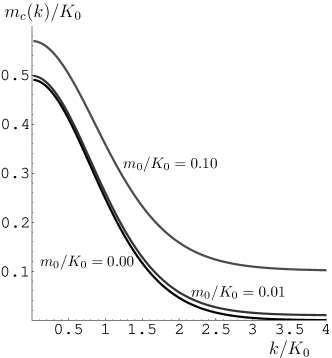
Figure 1: The constituent quark masses $m_{c}(k)$, solutions of the mass gap equation, for different current quark masses $m_{0}$.

The relativistic invariant Dirac-Feynman propagators Yaouanc , can be decomposed in the quark and antiquark Bethe-Goldstone propagators Bicudo_scapuz , used in the formalism of non-relativistic quark models,

$${\cal S}_{Dirac}(k_{0},\vec{k}) = {i\over\not k-m+i\epsilon}$$

$$= {i\over k_{0}-E(k)+i\epsilon}\ \sum_{s}u_{s}u^{\dagger}_{s}\beta$$

$$-{i\over-k_{0}-E(k)+i\epsilon}\ \sum_{s}v_{s}v^{\dagger}_{s}\beta\ ,$$

$$u_{s}({\bf k}) = \left[\sqrt{1+S\over 2}+\sqrt{1-S\over 2}\widehat{k}\cdot\vec{\sigma}\gamma_{5}\right]u_{s}(0)\ ,$$

$$v_{s}({\bf k}) = \left[\sqrt{1+S\over 2}-\sqrt{1-S\over 2}\widehat{k}\cdot\vec{\sigma}\gamma_{5}\right]v_{s}(0)\ ,$$ (3)

$$= -i\sigma_{2}\gamma_{5}u_{s}^{*}({\bf k})\ ,$$

where $S=\sin(\varphi)={m_{c}\over\sqrt{k^{2}+m_{c}^{2}}}\ ,\ C=\cos(\varphi)={k\over\sqrt{k^{2}+m_{c}^{2}}}$ and $\varphi$ is a chiral angle. In the non condensed vacuum, $\varphi$ is equal to $\arctan{m_{0}\over k}$. In the physical vacuum, the constituent quark mass $m_{c}(k)$, or the chiral angle $\varphi(k)=\arctan{m_{c}(k)\over k}$, is a variational function which is determined by the mass gap equation. We anticipate examples of solutions, for different light current quark masses $m_{0}$, depicted in Fig. 1.

There are three equivalent methods to derive the mass gap equation for the true and stable vacuum, where constituent quarks acquire the constituent mass Bicudo:2005de . One method consists in assuming a quark-antiquark ${}^{3}P_{0}$ condensed vacuum, and in minimizing the vacuum energy density. A second method consists in rotating the quark and antiquark fields with a Bogoliubov-Valatin canonical transformation to diagonalize the terms in the hamiltonian with two quark or antiquark second quantized fields. A third method consists in solving the Schwinger-Dyson equations for the propagators. Any of these methods lead to the same mass gap equation and quark dispersion relation. Here we replace the propagator of eq. (3) in the Schwinger-Dyson equation,

$$0=u_{s}^{\dagger}(k)\left\{k\widehat{k}\cdot\vec{\alpha}+m_{0}\beta-\int{dw^{\prime}\over 2\pi}{d^{3}k^{\prime}\over(2\pi)^{3}}iV(k-k^{\prime})\right.$$

$$\left.\sum_{s^{\prime}}\left[{u(k^{\prime})_{s^{\prime}}u^{\dagger}(k^{\prime})_{s^{\prime}}\over w^{\prime}-E(k^{\prime})+i\epsilon}-{v(k^{\prime})_{s^{\prime}}v^{\dagger}(k^{\prime})_{s^{\prime}}\over-w^{\prime}-E(k^{\prime})+i\epsilon}\right]\right\}v_{s^{\prime\prime}}(k)\ \$$

$$E(k)=u_{s}^{\dagger}(k)\left\{k\widehat{k}\cdot\vec{\alpha}+m_{0}\beta-\int{dw^{\prime}\over 2\pi}{d^{3}k^{\prime}\over(2\pi)^{3}}iV(k-k^{\prime})\right.$$

$$\left.\sum_{s^{\prime}}\left[{u(k^{\prime})_{s^{\prime}}u^{\dagger}(k^{\prime})_{s^{\prime}}\over w^{\prime}-E(k^{\prime})+i\epsilon}-{v(k^{\prime})_{s^{\prime}}v^{\dagger}(k^{\prime})_{s^{\prime}}\over-w^{\prime}-E(k^{\prime})+i\epsilon}\right]\right\}u_{s}(k),$$ (4)

where, with the simple density-density harmonic interaction Yaouanc , the integral of the potential is a laplacian and the mass gap equation and the quark energy are finally,

$$\Delta\varphi(k) = 2kS(k)-2m_{0}C(k)-{2S(k)C(k)\over k^{2}}$$ (5)

$$E(k) = kC(k)+m_{0}S(k)-{{\varphi^{\prime}(k)}^{2}\over 2}-{C(k)^{2}\over k^{2}}+{U\over 2}\ .$$

Numerically, this equation is a non-linear ordinary differential equation. It can be solved with the Runge-Kutta and shooting method. Examples of solutions for the current quark mass $m_{c}(k)=k\tan\varphi$, for different current quark masses $m_{0}$, are depicted in Fig. 1.

	$V^{++}=V^{--}$
spin-indep.	$-{d^{2}\over dk^{2}}+{{\bf L}^{2}\over k^{2}}+{1\over 4}\left({\varphi^{\prime}_{q}}^{2}+{\varphi^{\prime}_{\bar{q}}}^{2}\right)+{1\over k^{2}}\left({\cal G}_{q}+{\cal G}_{\bar{q}}\right)-U$
spin-spin	${4\over 3k^{2}}{\cal G}_{q}{\cal G}_{\bar{q}}{\bf S}_{q}\cdot{\bf S}_{\bar{q}}$
spin-orbit	${1\over k^{2}}\left[\left({\cal G}_{q}+{\cal G}_{\bar{q}}\right)\left({\bf S}_{q}+{\bf S}_{\bar{q}}\right)+\left({\cal G}_{q}-{\cal G}_{\bar{q}}\right)\left({\bf S}_{q}-{\bf S}_{\bar{q}}\right)\right]\cdot{\bf L}$
tensor	$-{2\over k^{2}}{\cal G}_{q}{\cal G}_{\bar{q}}\left[({\bf S}_{q}\cdot\hat{k})({\bf S}_{\bar{q}}\cdot\hat{k})-{1\over 3}{\bf S}_{q}\cdot{\bf S}_{\bar{q}}\right]$
	$V^{+-}=V^{-+}$
spin-indep.	$0$
spin-spin	$-{4\over 3}\left[{1\over 2}{\varphi^{\prime}_{q}}{\varphi^{\prime}_{\bar{q}}}+{1\over k^{2}}{\cal C}_{q}{\cal C}_{\bar{q}}\right]{\bf S}_{q}\cdot{\bf S}_{\bar{q}}$
spin-orbit	$0$
tensor	$\left[-2{\varphi^{\prime}_{q}}{\varphi^{\prime}_{\bar{q}}}+{2\over k^{2}}{\cal C}_{q}{\cal C}_{\bar{q}}\right]\left[({\bf S}_{q}\cdot\hat{k})({\bf S}_{\bar{q}}\cdot\hat{k})-{1\over 3}{\bf S}_{q}\cdot{\bf S}_{\bar{q}}\right]$

Table 1: The positive and negative energy spin-independent, spin-spin, spin-orbit and tensor potentials, computed exactly in the framework of the simple density-density harmonic model of eq. (2). $\varphi^{\prime}(k)$, ${\cal C}(k)$ and ${\cal G}(k)=1-S(k)$ are all functions of the constituent quark(antiquark) mass.

The Salpeter-RPA equations for a meson (a colour singlet quark-antiquark bound state) can be derived from the Lippman-Schwinger equations for a quark and an antiquark, or replacing the propagator of eq. (3) in the Bethe-Salpeter equation. In either way, one gets Bicudo_scapuz

$$\phi^{+}(k,P) = {u^{\dagger}(k_{1})\chi(k,P)v(k_{2})\over+M(P)-E(k_{1})-E(k_{2})}$$

$${\phi^{-}}^{t}(k,P) = {v^{\dagger}(k_{1})\chi(k,P)u(k_{2})\over-M(P)-E(k_{1})-E(k_{2})}$$

$$\chi(k,P) = \int{d^{3}k^{\prime}\over(2\pi)^{3}}V(k-k^{\prime})\left[u(k^{\prime}_{1})\phi^{+}(k^{\prime},P)v^{\dagger}(k^{\prime}_{2})\right.$$ (6)

$$\left.+v(k^{\prime}_{1}){\phi^{-}}^{t}(k^{\prime},P)u^{\dagger}(k^{\prime}_{2})\right]$$

where $k_{1}=k+{P\over 2}\ ,\ k_{2}=k-{P\over 2}$ and $P$ is the total momentum of the meson.

The Salpeter-RPA equations of PB et al. Bicudo_thesis and of Llanes-Estrada et al. Llanes-Estrada_thesis are obtained deriving the equation for the positive energy wavefunction $\phi^{+}$ and for the negative energy wavefunction $\phi^{-}$. Solving for $\chi$, one gets the Salpeter equations of Le Yaouanc et al. Yaouanc . This results in four potentials $V^{\alpha\beta}$ respectively coupling $\nu^{\alpha}=r\phi^{\alpha}$ to $\nu^{\beta}$, in the boundstate Salpeter equation,

$$\left\{\begin{array}[]{rrr}\left(2T+V^{++}\right)\,\nu^{+}\ +&V^{+-}\ \ \nu^{-}=&M\nu^{+}\\ V^{-+}\ \ \nu^{+}\ +&\left(2T+V^{--}\right)\,\nu^{-}=&-M\nu^{-}\end{array}\right..$$ (7)

The relativistic equal time equations have the double of coupled equations than the Schrödinger equation. The negative energy component $\nu^{-}$ is smaller than the positive energy component by a factor of the order of $1/M$ in units ok $K_{0}=1$. Thus when $M$ is large, and this is the case for most excited mesons, the negative energy components can be neglected and the Salpeter equation simplifies to a Schrödinger equation.

Importantly, the potentials $V^{++}=V^{--}$ and $V^{+-}=V^{-+}$ include the usual spin-tensor potentials Bicudo_baryon , produced by the Pauli $\vec{\sigma}$ matrices in the spinors of eq. (3). They are detailed explicitly in Table 1. Because we are interested in highly excited states, where both $\langle r\rangle$ and $\langle k\rangle$ are large, we consider the limit where ${m_{c}\over k}\rightarrow 0$. This implies that the potentials, used in Table 1, $\varphi^{\prime}(k)\rightarrow 0$, ${\cal C}(k)\rightarrow 1$ and ${\cal G}(k)=1-S(k)\rightarrow 1$. Then using the textbook matrix elements of the spin-tensor potentials, the boundstate Salpeter equation decouples in two different equations depending only on $\mathbf{J}$ and not explicitly on $\mathbf{L}$ or $\mathbf{S}$. Without the chiral degeneracy there would be four different resonances for each $j$, one with $s=0$ and $j=l$ and three with $s=1$ and $j=l-1,\,l,\,l+1$. With the chiral degeneracy we get only two different equations, one for $j\geq 0$ with,

$$\left\{\begin{array}[]{cl}2T+V^{++}=&-{d^{2}\over dk^{2}}+2k-{1\over k^{2}}+{j(j+1)\over k^{2}}\\ V^{+-}=&{1\over k^{2}}\\ \end{array}\right.\ ,$$ (8)

and another for $j\geq 1$ with,

$$\left\{\begin{array}[]{cl}2T+V^{++}=&-{d^{2}\over dk^{2}}+2k-{2\over k^{2}}+{j(j+1)\over k^{2}}\\ V^{+-}=&{0\over k^{2}}\\ \end{array}\right.\ .$$ (9)

Thus states with different $l$ and equal $j$, i.e. with different parity are degenerate, and chiral symmetry is restored. This chiral degeneracy applies to all angular momenta, except for $j=0$. In Table 2 we show the masses of the different light-light mesonic solutions of eqs. (8) and (9), including tachyons, corresponding to the limit where $m_{c}<<k$.

n	Pse	Sca	j=1	j=1	j=2	j=2	j=3	j=3
0	$2\times 10^{-1}i\over m^{2}$	$3\times 10^{-2}i\over m^{2}$	3.71	4.59	6.15	6.45	7.65	7.84
1	$2\times 10^{-3}i\over m^{2}$	$3\times 10^{-4}i\over m^{2}$	6.49	7.15	8.43	8.69	9.72	9.89
2	$2\times 10^{-5}i\over m^{2}$	$3\times 10^{-6}i\over m^{2}$	8.76	9.32	10.45	10.68	11.61	11.76
3	$2\times 10^{-7}i\over m^{2}$	$3\times 10^{-8}i\over m^{2}$	10.77	11.27	12.30	12.51	13.38	13.52
4	$2\times 10^{-9}i\over m^{2}$	$3\times 10^{-10}i\over m^{2}$	12.61	13.08	14.05	14.25	15.12	15.26

Table 2: Masses of the first angular and radial excitations of the different light-light tachyons and mesons in the chiral limit of $m<<k$. Each column includes both positive and negative parity degenerate states, except for the pseudoscalar and scalar tachyonic states. The meson masses are separated in two different families with the same $J$ because two different Salpeter equations (8) and (9) exist for each $J$.

The $j=0$ case is a subtle one, because neglecting the mass $m_{c}$ is equivalent to consider the chiral limit, and this is equivalent to change from the physical vacuum to the chiral invariant vacuum which is a false, unstable vacuum. A detailed inspection shows that the different potentials $-{d^{2}\over dk^{2}}\,,\ 2k\,,\ {1\over k^{2}}$ are bound from below and positive definite in the sense that all their eigenvalues are positive. However $-{1\over k^{2}}$ is unbound from below. It turns out that for $j=0$ all the solutions of eq. (8), including all radial excitations, are tachyons Bicudo:2006dn , relevant for the structure of the chiral invariant false vacuum of QCD Hiller , corresponding to a different solution of the mass gap equation $m_{c}=0$. Even when a very small regularizing quark mass $m_{c}$ is assumed, constant for simplicity, the tachyons persist. This is confirmed by the numerical solutions of the regularized Salpeter equation, shown in Table 2 . Technically, in the $j=0$ case, it is necessary to rescale the momentum and mass,

$$k/m_{c} \rightarrow {k^{\prime}}\ ,$$

$$M\,{m_{c}}^{2} \rightarrow M^{\prime}\ ,$$ (10)

where any finite solution $M^{\prime}$ in fact corresponds to a large mass $M=M^{\prime}/m_{c}^{2}$, and where a wave-function with a finite $k^{\prime}$ corresponds to a wave-function with small momentum $k=k^{\prime}\,m_{c}$. A long time ago Le Yaouanc et al. Yaouanc showed that in the chiral limit the pseudoscalar and the scalar possess tachyonic solutions. Very recently PB showed that this number of tachyons is infinite Bicudo:2006dn . Only with a finite $m_{c}$ quark mass, do the scalar and pseudoscalar mesons have positive masses. But then the excited scalar and pseudoscalar states are not degenerate, in contradistinction with the chiral degeneracy of the excited mesons with $j>0$.

For excited mesons with $j>0$, the spectrum in table 2 is very well aproximated by the solutions of the pair of Schrödinger-like equations,

$$\left[-{d^{2}\over dk^{2}}+2k-{1\over k^{2}}+{j(j+1)\over k^{2}}\right]\nu(k) = M\nu(k)$$ (11)

$$\left[-{d^{2}\over dk^{2}}+2k-{2\over k^{2}}+{j(j+1)\over k^{2}}\right]\nu(k) = M\nu(k)$$ (12)

obtained when the negative energy component $\nu^{-}$ are neglected in eqs (8) and (9).

III Linear Regge trajectories and semi-classical quantization

The simple quadratic model is now extended to a linear potential Llanes-Estrada_thesis ; Bicudo_KN , to get the linear Regge trajectories. It is well known, both from the quark modelling of the hadronic spectra, and from Lattice QCD, that the long range confining quark potential is linear. Notice that Szczepaniak et. al. Szczepaniak , in the coulomb gauge, were able to derive from QCD the linear potential. Continuing with the limit where ${m\over k}\rightarrow 0$, we assume the radial equation,

$$p = \sqrt{-{d^{2}\over dr^{2}}+{j(j+1)\over r^{2}}}$$

$$\left(p+\sigma\ r\right)\nu(r) = E\nu(r)\ ,$$ (13)

where the negative energy components (vanishing with $1\over M$) were neglected, and where the terms similar to the terms $-1\over k^{2}$ or $-2\over k^{2}$ of eq. (11) or eq. (12)were also neglected. We only expect these approximations to be reasonable for highly excited states, and for $j>0$ because the number of excited false vacua remains infinite Bicudo_rep .

Then we have to solve a Salpeter equation (or Schrödinger equation with ultrarelativistic kinetic energy) except that the spherical angular momentum $l$ is now replaced by the total angular momentum $j$, in the centrifugal barier. Eq.(13) is solved with the method of the double diagonalization of the equal time hamiltonian. Using finite differences, first we diagonalize the bounded from below operator $-{d^{2}\over dr^{2}}+{j(j+1)\over r^{2}}$ . Then we apply the square root. After returning to the original position space basis, we diagonalize the full hamiltonian. This provides us automatically with the full spectrum including the angularly and radially excited states.

$j$	$n$=0	$n$=1	$n$=2	$n$=3	$n$=4	$n$=5	$n$=6	$n$=7	$n$=8
0	3.16	4.71	5.89	6.87	7.73	8.51	9.21	9.87	10.49
1	4.22	5.46	6.48	7.38	8.17	8.90	9.58	10.21	10.81
2	5.08	6.13	7.05	7.87	8.61	9.30	9.95	10.56	11.13
3	5.81	6.74	7.58	8.34	9.04	9.70	10.31	10.90	11.45
4	6.46	7.31	8.08	8.79	9.45	10.08	10.67	11.23	11.77
5	7.05	7.83	8.55	9.22	9.86	10.45	11.02	11.56	12.08
6	7.60	8.32	9.00	9.64	10.24	10.82	11.36	11.89	12.39
7	8.11	8.79	9.43	10.04	10.62	11.17	11.70	12.21	12.70
8	8.59	9.23	9.84	10.43	10.98	11.51	12.03	12.52	12.99
9	9.04	9.65	10.24	10.80	11.33	11.85	12.34	12.82	13.29
10	9.47	10.06	10.62	11.16	11.68	12.18	12.66	13.12	13.58
11	9.88	10.45	10.99	11.51	12.01	12.49	12.96	13.42	13.86
12	10.28	10.82	11.35	11.85	12.34	12.81	13.26	13.71	14.14
13	10.66	11.19	11.69	12.18	12.65	13.11	13.56	13.99	14.41

Table 3: Masses of the light-light mesons, in dimensionless units of $\sigma=1$, computed with the ultrarelativistic equal time chiral degenerate Schrödinger equation (13). The $j=0$ mesons are distant from the experimental spectrum, but chiral degeneracy is theoretically plausible for the very excited mesons.

The results are shown in Table 3. In Fig. 2 and in Fig. 3 we graphically demonstrate that the angular excitations and the radial excitations of this simple spectrum are disposed in linear Regge trajectories,

$$j \simeq \alpha_{0}+\alpha M^{2}\ ,$$

$$j \simeq \beta_{0}+\beta M^{2}\ .$$ (14)

This agrees qualitatively with the experimental spectrum Bugg:2004xu , where the linear Regge trajectories are also present.

Interestingly, with the semi-classical Bohr-Sommerfeld quantization relation

$$\oint p\ dq\simeq n\,h\ ,$$ (15)

and with the energy $2p\,c+\sigma\,r$ of eq. (13) the linear trajectories can be derived. The linear trajectories for the angular excitations can be derived from the circular classical orbits,

$$\left\{\begin{array}[]{rcl}2\left(2\pi\,{r\over 2}\,p\right)&\simeq&l\,h\\ \sigma&=&{\ \scriptstyle c\ \over{\scriptstyle r\over\scriptstyle 2}}p\end{array}\right.$$ (18)

$$\Rightarrow l\simeq{1\over 8\sigma c\,\hbar}E^{2}\ ,$$ (19)

where we also used the centripetal acceleration. The linear trajectories corresponding to radial excitations can be derived Arriola:2006sv from the linear classical orbits with $\mathbf{L}=0$,

$$\int_{-E/\sigma}^{E/\sigma}{E-\sigma|r|\over 2c}dr\simeq n\,h$$ (20)

$$\Rightarrow n\simeq{1\over 4\pi\sigma c\,\hbar}E^{2}\ .$$

Thus, in our units of $\hbar=c=\sigma=1$ we get for the Regge slopes respectively,

$$\alpha = {1\over 8}\ ,$$

$$\beta = {1\over 4\pi}\ ,$$ (21)

in excelent agreement with the slopes of Figs. 2 and 3, and similar to a recent Bethe-Salpeter calculation Wagenbrunn:2007ie .

Although the simplified model of eq. (13) agrees qualitatively with the experiment, both in the chiral degeneracy and in the linear Regge trajectories, there are quantitative discrepancies. In particular, experimentally, the radial and agular slopes defined in eq. (14) should be almost identical Bugg:2004xu ,

$$\alpha_{\mbox{exp}} = 0.877\ \mbox{GeV}^{-2}\ ,$$

$$\beta_{\mbox{exp}} = 0.855\ \mbox{GeV}^{-2}\ ,$$ (22)

while our theoretical slopes, depicted in Figs. 2 and 3 and semi-classically computed in eq. (21), differ by $\pi/2$. Moreover the meson masses in Table 3 do not exactly comply with the large degeneracy emerging in the observations of Bugg.

Figure 2: We show the quasi-linear Regge trajectories, of $j$ as a function of $M^{2}$. Each line corresponds to a fixed radial $n$, increasing from left to right. The $M$ are the masses of the light-light mesons, in dimensionless units of $\sigma=1$, computed with the ultrarelativistic equal time chiral degenerate Schrödinger equation (13).

IV Searching for a principal quantum number with classical closed orbits

To better model the large degeneracy, we enlarge our class of time-like central potentials, searching for the best possible potential of this class. Actually the model of Section III, with a linear potential only, is oversimplified. To fit the correct positive intercepts $\alpha_{0}$ and $\beta_{0}$ of eq. (14), it is standard in quark models to include in the potential a constant negative energy shift and a negative short range Coulomb potential.

To exactly reproduce the large degeneracy, we ask for a spectrum with a principal quantum number, similar to the non-relativistic spectra of the Coulomb potential or of the harmonic oscillator potential, where the principal quantum numbers are respectively $n+l+1$ and $2n+l+{3\over 2}$. The difference here is that our kinetic energy is the ultrarelativistic one $T=2\,p\,c$ whereas in the non-relativistic case $T={p^{2}\over 2\mu}$.

Notice that in the non-relativistic case, classical closed orbits coincide with a quantum principal number. We can also address this problem searching for classical closed orbits with an ultrarelativistic kinetic energy. When all the classical orbits are closed then the Hermann-Jacobi-Laplace-Runge-Lenz vector is conserved, because this vector does not precess. In the Hamilton-Jacobi formalism, this vector commutes with the hamiltonian. The same commutation then also occurs in the quantum Schrödinger formalism, the formalism we are using now. Then a larger symmetry group, including the angular momentum and the Hermann-Jacobi-Laplace-Runge-Lenz vector exists. Finally this implies that a principal quantum number exists.

Thus, rather than solving the ultrarelativistic Schrödinger equation for all the infinite possible central potentials, we prefer to extend the Bertand theorem techniques to the search of classical closed orbits with the ultrarelativistic kinetic energy. For simplicity we consider a kinetic energy $T=p\,c$ and a general potential $V(r)$, used for a single particle in a central potential, comparable to our two-body problem in the centre of mass frame.

Figure 3: We show we show the quasi-linear Regge trajectories, of $n$ as a function of $M^{2}$. Each line corresponds to a fixed angular $j$, increasing from left to right. The $M$ are the masses of the light-light mesons, in dimensionless units of $\sigma=1$, computed with the ultrarelativistic equal time chiral degenerate Schrödinger equation (13).

Let us consider classical planar trajectories for an ultrarelativistic quark with the speed of light, and with momentum,

$$\mathbf{p} = {p\over c}\mathbf{v}$$ (23)

$$= {p\over c}\,\dot{r}\,\widehat{e}_{r}+{p\over c}r\,\dot{\theta}\,\widehat{e}_{\theta}\ ,$$

subject to a central force,

$$\mathbf{F}=-{d\over dr}V\,\widehat{e}_{r}\ ,$$ (24)

where the notation is obvious. In the plane we have two constants, the angular momentum $L$ and the energy $E$,

$$\mathbf{L} = {p\over c}\,r^{2}\,\dot{\theta}\,\widehat{e}_{\perp}\ \ ,$$

$$E = p\,c+V(r)\ \ .$$ (25)

Then Newton’s law produces the equation for the radius as a function of time,

$$\left({E-V\over c^{2}}\dot{r}\right)^{\displaystyle\dot{}}-{L^{2}\over{E-V\over c^{2}}r^{3}}=-{d\over dr}V\ \ .$$ (26)

To study the condition to get closed orbits it is convenient to relace the variable time $t$ by the polar coordinate $\theta$ and the function $r$ by it’s inverse $u=1/r$. Then the equation simplifies to,

$${d^{2}\over d\theta^{2}}u+u = J(u)$$

$$J(u) = -{E-V(1/u)\over c^{2}L^{2}}{d\over du}V(1/u)\ \ .$$ (27)

To get the classical case one only has to replace in the right hand side of eq. (27) the factor ${E-V(1/u)\over c^{2}}\rightarrow m$. Thus the ultrarelativistic case has two independent constants $E$ and $cL$ while the classical case has only one constant $m/L$.

The theorem of Bertrand can be addressed considering a trajectory $u$ close to the circular trajectory $u_{0}$,

$$u=u_{0}+\eta\ \ ,$$ (28)

where we fix the angular momentum $L$ and the trajectory is defined by the inverse radius $u$ and derivative at $\theta=0$ and by the energy $E$. Defining,

$$\beta^{2}=1-{d\over du}J|_{u=u_{0}}\ \ ,$$ (29)

we get, to leading order in $\eta$,

$${d^{2}\eta\over d\theta^{2}}+\beta^{2}\eta = 0$$

$$\eta = h_{1}\,\cos\beta(\theta-\theta_{0})\ \ .$$ (30)

Thus for very small perturbations to the circular orbit, the condition for a closed orbit is that $\beta$ is an integer number (if we want the orbit to close right after one turn) or rational (if we want it to close after a finite number of turns). Importantly this implies that $\beta$ is constant, since it can’t change continuously from one orbit with $u_{0}$ to the next one. This restricts the class of possible potentials,

$${d\over du}J|_{u=u_{0}} = 1-\beta^{2}$$ (31)

$$= {f^{2}({1\over u_{0}})\over c^{2}L^{2}{u_{0}}^{2}}-2+{u_{0}\over f_{0}}{df({1\over u_{0}})\over du_{0}}$$

and the problem here is that, unlike in the non-relativistic limit, the equation still depends on the parameter $cL$, and thus the closed orbits are possible, but there is no potential for which all orbits are closed, since the closing depends on $cL$.

In the non-relativistic case it is well known that this problem has two solutions because the first term in the right-hand-side is absent. Then the solutions of eq. (31), producing closed orbits close to the circular one, are the power law potential with $V(r)\alpha r^{\beta^{2}-2}$. For instance the natural $\beta$ correspond to the powers -1, 2, 7, 14 … For more general orbits, we can go up to the third order in the Fourier series for $\eta$,

$$\eta=h_{0}+h_{1}\,\cos\beta\theta+h_{2}\,\cos 2\beta\theta+h_{3}\,\cos 3\beta\theta$$ (32)

and this already produces Bertrand’s theorem, stating that the closed orbit condition is,

$$\beta^{2}(\beta^{2}-1)(\beta^{2}-4)=0$$ (33)

This includes only the Coulomb and the harmonic oscillator cases, which indeed have all orbits simply closed for a non-relativistic kinetic energy.

Again, for an ultrarelativistic kinetic energy there is no potential with all orbits closed.

V Conclusion

Here we study possible quark models for the large degeneragy in the meson spectra reported by Bugg Bugg:2004xu .

We start with a semi-relativistic chiral invariant quark model, with relativistic kinetic energy, with negative energy components, but with an instantaneous potential. For excited states all the different spin-tensor potentials Bicudo_scalar ; Llanes-Estrada_hyperfine ; Villate merge and we arrive at a schrödinger-like ultrarelativistic linear potential quark model with a simple $\mathbf{J}^{2}$ dependence. Although the chiral degeneracy is expected to only dominate the high excitations, this schrödinger-like quark model is conveniently simple to address the large degeneracy.

The most ambitious approach to the large degeneracy consists in asking for a model with a principal quantum number. Notice that when the corresponding classical orbits are all closed, the Hermann-Jacobi-Laplace-Runge-Lenz vector is conserved. In quantum mechanics this corresponds to a larger symmetry, both angular and dynamical, and to a single principal quantum number that encompasses both the angular and radial excitations. Unfortunately we find that this is not possible in our ultrarelativistic and instantaneous framework.

Another possible approach is the one of an approximate large degeneracy. The linear and radial excitations are so regular in the framework of the ultrarelativistic and equal time quark model that approximate patterns occur in the spectrum. Notice that in eq. (21), in Figs. 2 and 3, and in Table 3, an increment of 3 in $j$ is approximately equivalent to an increment of 2 in $n$. For instance the meson with $j=5,\,n=0$ has a similar mass to the one with $j=2,\,n=3$. Notice that the $j=5$ state may have $l=4,\,5,$ or 6, while the $j=2$ state may have $l=1,\,1,$ or 3. we get an approximate but relatively large degeneracy of states with different $l$ ranging from 1 to 6. To agree with the experiment, we only need to have an increment in $n$ much closer to the increment in $j$.

Thus, both for the principal quantum number, and for an approximate degeneracy, a departure from the ultrarelativistic and equal time quark model is necessary. It is plausible that either retardation, string effects, or coupled channel effects should improve the theoretical model. For instance Morgunov et al. Morgunov:1999fj already showed that including the angular momentum of the rotating linear confining string changes the slopes of the angular Regge trajectories. Moreover, if one could succeed to include retardation properly in the confining quark model, then one might search again for the possible existence of a principal quantum number. And coupled channels might also affect differently the angular and radial excitations of the spectrum.

In any case the large degeneracy apparent in the data analysis of Bugg, supported by the solid pattern of linear angular and radial Regge trajectories, remains quite plausible from a theoretical perspective. More experimental data on the remarkable patterns of excited resonances is welcome.

- (1) D. V. Bugg, Phys. Rept. 397, 257 (2004) [arXiv:hep-ex/0412045].
- (2) S. S. Afonin, Phys. Lett. B 639, 258 (2006) [arXiv:hep-ph/0603166]; S. S. Afonin, Eur. Phys. J. A 29, 327 (2006) [arXiv:hep-ph/0606310]; S. S. Afonin, arXiv:hep-ph/0701089.
- (3) L. Y. Glozman, arXiv:hep-ph/0701081.
- (4) The large degeneracy is clear in Fig.1 of Ref Afonin:2006vi b and in Fig. 2 of Ref Glozman:2007ek .
- (5) E. Aker et al. [Crystal Barrel Collaboration], Nucl. Instrum. Meth. A 321 (1992) 69.
- (6) G. F. Chew and S. C. Frautschi, Phys. Rev. Lett. 7, 394 (1961).
- (7) R. Fiore, L. L. Jenkovszky, F. Paccanoni and A. Prokudin, Phys. Rev. D 70, 054003 (2004) [arXiv:hep-ph/0404021].
- (8) W. M. Yao et al. [Particle Data Group], J. Phys. G 33 (2006) 1.
- (9) A. V. Anisovich et al., Phys. Lett. B 517 (2001) 261. 5Wagenbrunn:2007ie
- (10) R. F. Wagenbrunn and L. Y. Glozman, Phys. Rev. D 75, 036007 (2007) [arXiv:hep-ph/0701039];
- (11) T. Burch, C. Gattringer, L. Y. Glozman, C. Hagen, D. Hierl, C. B. Lang and A. Schafer, Phys. Rev. D 74, 014504 (2006) [arXiv:hep-lat/0604019]; T. Burch, C. Gattringer, L. Y. Glozman, C. Hagen, C. B. Lang and A. Schafer, Phys. Rev. D 73, 094505 (2006) [arXiv:hep-lat/0601026]; T. D. Cohen and L. Y. Glozman, Phys. Rev. D 65, 016006 (2002) [arXiv:hep-ph/0102206].
- (12) A. Le Yaouanc, L. Oliver, S. Ono, O. Pene and J. C. Raynal, Phys. Rev. D 31, 137 (1985); A. Amer, A. Le Yaouanc, L. Oliver, O. Pene and J. C. Raynal, Phys. Rev. Lett. 50, 87 (1983); A. Le Yaouanc, L. Oliver, O. Pene and J. C. Raynal, Phys. Rev. D 29, 1233 (1984); A. Le Yaouanc, L. Oliver, O. Pene and J. C. Raynal, Phys. Lett. B 134, 249 (1984); A. Amer, A. Le Yaouanc, L. Oliver, O. Pene and J. C. Raynal, Phys. Rev. D 28, 1530 (1983).
- (13) P. Bicudo and J. E. Ribeiro, Phys. Rev. D 42, 1611 (1990); Phys. Rev. D 42, 1625; Phys. Rev. D 42, 1635.
- (14) P. Bicudo, N. Brambilla, E. Ribeiro and A. Vairo, Phys. Lett. B 442, 349 (1998) [arXiv:hep-ph/9807460].
- (15) M. Malheiro, private communication (1999).
- (16) U.Thoma, “Recent results from the Crystal Barrel experiment at ELSA,” presented at the International Workshop XXXIV on Gross Properties of Nuclei and Nuclear Excitations, Hirschegg, (2007)
- (17) P. Bicudo, Phys. Rev. D 74, 036008 (2006) [arXiv:hep-ph/0512041].
- (18) H. G. Dosch and Y. A. Simonov, Phys. Lett. B 205, 339 (1988);
- (19) Y. S. Kalashnikova, A. V. Nefediev and J. E. F. Ribeiro, Phys. Rev. D 72, 034020 (2005) [arXiv:hep-ph/0507330].
- (20) A. V. Nefediev, JETP Lett. 78, 349 (2003) [Pisma Zh. Eksp. Teor. Fiz. 78, 801 (2003)] [arXiv:hep-ph/0308274].
- (21) P. Bicudo, Phys. Rev. C 60, 035209 (1999).
- (22) F. J. Llanes-Estrada and S. R. Cotanch, Phys. Rev. Lett. 84, 1102 (2000) [arXiv:hep-ph/9906359].
- (23) P. Bicudo, G. Krein, J. E. F. Ribeiro and J. E. Villate, Phys. Rev. D 45, 1673 (1992).
- (24) P. Bicudo, Phys. Rev. D 74, 065001 (2006) [arXiv:hep-ph/0606189].
- (25) A. A. Osipov, B. Hiller, V. Bernard and A. H. Blin, arXiv:hep-ph/0507226; A. A. Osipov, B. Hiller and J. da Providencia, Phys. Lett. B 634, 48 (2006) [arXiv:hep-ph/0508058]; A. A. Osipov, B. Hiller, J. Moreira and A. H. Blin, Eur. Phys. J. C 46, 225 (2006) [arXiv:hep-ph/0601074]; B. Hiller, A. A. Osipov, V. Bernard and A. H. Blin, SIGMA 2, 026 (2006) [arXiv:hep-ph/0602165].
- (26) P. Bicudo, J. E. Ribeiro and J. Rodrigues, Phys. Rev. C 52, 2144 (1995).
- (27) A. P. Szczepaniak and E. S. Swanson, Phys. Rev. D 65, 025012 (2002) [arXiv:hep-ph/0107078]; A. P. Szczepaniak and E. S. Swanson, Phys. Rev. Lett. 87, 072001 (2001) [arXiv:hep-ph/0006306]; A. P. Szczepaniak and E. S. Swanson, Phys. Rev. D 62, 094027 (2000) [arXiv:hep-ph/0005083];
- (28) P. J. A. Bicudo and A. V. Nefediev, Phys. Rev. D 68, 065021 (2003) [arXiv:hep-ph/0307302].
- (29) E. R. Arriola and W. Broniowski, arXiv:hep-ph/0609266.
- (30) P. Bicudo and G. Marques, Phys. Rev. D 70, 094047 (2004) [arXiv:hep-ph/0305198].
- (31) F. J. Llanes-Estrada and S. R. Cotanch, Nucl. Phys. A 697, 303 (2002) [arXiv:hep-ph/0101078]; F. J. Llanes-Estrada, S. R. Cotanch, A. P. Szczepaniak and E. S. Swanson, Phys. Rev. C 70, 035202 (2004) [arXiv:hep-ph/0402253].
- (32) J. E. Villate, D. S. Liu, J. E. Ribeiro and P. Bicudo, Phys. Rev. D 47, 1145 (1993).
- (33) V. L. Morgunov, A. V. Nefediev and Yu. A. Simonov, Phys. Lett. B 459, 653 (1999) [arXiv:hep-ph/9906318].