On the Existence of Angular Correlations in Decays with Heavy Matter Partners

Abstract:

If heavy partners of the Standard Model matter fields are discovered at the LHC it will be imperative to determine their spin in order to uncover the underlying theory. In decay chains, both the spin and the mass hierarchy of all particles involved can influence the resulting angular correlations. We present the necessary conditions for decays involving the matter partners to exhibit angular correlations. In particular we find that when the masses are not degenerate, a heavy fermionic sector always displays angular correlations in cascade decays. When the masses are closely degenerate the size of spin effects is controlled by a global phase parameter. In a large region of the parameter space, correlations are strongly suppressed. In other regions, such as in UED model where this phase is fixed by 5-d Lorentz invariance, the correlations are pronounced. In addition, we show that in certain cases one may even have enough information to determine the spin of other heavy partners involved in the decay (such as the Lightest Stable Partner or a heavy gluon).

1 Introduction

Stabilizing the hierarchy between the electroweak (EW) scale and the Planck scale generically requires the existence of new particles at the TeV scale. Typically, such new particles organize themselves into partners of the Standard Model (SM) particles, i.e. they have the same gauge quantum numbers. However, the spin of such partners is more model dependent. There exist models where the partners’ spin is opposite to that of the SM particles (the prime example is of course Supersymmetry). There are also several other models where the partners’ spin is the same as that of the SM particles (e.g. UED [1, 2] or Little Higgs models[3, 4, 5, 6, 7, 8, 9])

Recently, numerous papers began to address the issue of direct spin determination at the LHC. The comparison was usually made between Supersymmetry (SUSY) and the Universal Extra-dimensions (UED) scenario [10, 11, 12, 13, 14, 15, 16]. In this paper we would like to point out general features of any such comparison which go beyond the particular model of UED (see also [17, 18, 19]).

We begin by analyzing the case of fermionic partners of SM matter fields (i.e. quarks and leptons) with a general mass spectrum and model independent couplings. As we emphasized in a previous publication [18] the chirality of the couplings is a crucial ingredient in any attempt at spin determination. We give a complete description of the necessary conditions for chiral couplings of the new matter sector. These conditions depend strongly on the spectrum. We identify the relevant parameters to be the relative size of the splitting between the Dirac masses $\Delta M$ and the Yukawa mass $\sim\lambda v$. In the case where there is a large splitting between the partners of the left and right handed SM fields, the interactions are dominantly chiral.

However, when the matter partners’ spectrum is closely degenerate, the situation is more subtle. The chirality of the coupling is controlled by a phase parameter in the fermionic mass matrix. It interpolates between a limit where the chiral coupling is suppressed and one where the chiral coupling is enhanced. For the UED model this phase is fixed by 5-d Lorentz invariance and leads to an enhanced chiral structure. However, in principle the situation could be very different for a general model of fermionic partners of the matter sector (e.g. Little Higgs). We examine the consequences of a general phase structure on the prospects of spin determination.

In light of these observations it becomes clear that rather than treating UED as a universal benchmark, studies of spin correlations should extend to models with more general fermionic couplings. Due to the close connection between chirality and 5-d Lorentz invariance, this also means that experimental observation of degenerate fermion partners with chiral couplings provides a unique test of models based on extra dimensions.

In addition, we investigate the possibility of extracting further information from a decay involving the matter partners. We will consider event topologies as shown in Fig.1 where $F$ is the matter partner. If $F$ is a scalar, Lorentz invariance constrains $X$ and $Y$ to be fermions. Since there is no correlation between the outgoing $f-\bar{f}$ to begin with, one cannot hope to extract any more information. In contrast, when $F$ is a fermion, $X$ and $Y$ can be either a scalar or a vector-boson. We discuss the dependence of the $f-\bar{f}$ angular correlation on the spin of $X$ and $Y$ and show that, with sufficient information regarding the mass spectrum, one can unambiguously determine the spin of $X$ and $Y$.

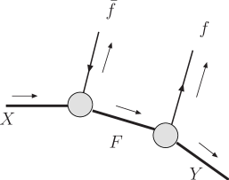
Figure 1: The topology for a generic decay where spin information may be found. A heavy particle $X$ decays into a SM fermion $\bar{f}$ and a heavy partner $F$ which subsequently decays into another SM fermion $f$ and an invisible particle $Y$. The angular correlations between $f$ and $\bar{f}$ may reveal the spin identity of the intermediate particle $F$.

The paper is organized as follows: In section 2 we lay down the necessary conditions for having chiral vertices in the heavy matter sector with fermionic partners of the SM and in section 3 we discuss the resulting angular correlations in cascade decays involving the SM matter partners. In section 4 we focus on additional information that can be extracted out of such cascade decays. Section 5 contains a brief discussion of some experimental difficulties such measurements must confront. In section 6 we present our conclusions.

2 Chirality Conditions

In this section we discuss the conditions needed for a heavy fermionic sector to have chiral couplings with the SM fields. We will assume that this new sector has the same quantum numbers as the known quarks and leptons. In addition, we will assume that some $Z_{2}$ parity symmetry is present (e.g. $KK$-parity in the UED model or $T$-parity in Little Higgs models). We will use the quark sector to demonstrate our results, but it should be clear that identical conclusions apply to the lepton sector as well.

SM	Heavy partners	$SU(2)\times U_{Y}(1)$
$q_{L}$	$Q_{L}^{\prime}=\left(\begin{array}[]{l}u_{L}^{\prime}\\ d_{L}^{\prime}\\ \end{array}\right)\quad Q_{R}^{\prime}=\left(\begin{array}[]{l}u_{R}^{\prime}\\ d_{R}^{\prime}\\ \end{array}\right)$	$\left(2,\frac{1}{6}\right)$
$u_{R}$	$U_{R}^{\prime}\hskip 62.59596ptU_{L}^{\prime}$	$\left(1,\frac{2}{3}\right)$
$d_{R}$	$D_{R}^{\prime}\hskip 62.59596ptD_{L}^{\prime}$	$\left(1,-\frac{1}{3}\right)$

We denote the heavy fermionic modes by $Q_{L,R}^{\prime}$, $U_{L,R}^{\prime}$ and $D_{L,R}^{\prime}$ (for simplicity we are considering only one generation). Here, $Q^{\prime}=(u^{\prime},d^{\prime})$ is an $SU(2)$ doublet while $U^{\prime}$ and $D^{\prime}$ are singlets; note that $Q_{L}^{\prime}$,$U_{R}^{\prime}$ and $D_{R}^{\prime}$ are partners to SM fermions while $Q_{R}^{\prime}$,$U_{L}^{\prime}$ and $D_{L}^{\prime}$ have no low energy counterparts.

Due to the $Z_{2}$ parity, the heavy fermions can only couple to the SM via heavy bosons ($g^{\prime}$, $Z^{\prime}$ and etc.). The chiral nature of the SM restricts the form of the interactions. For example, the couplings to the heavy gluon $g^{\prime}$ is

$$\mathcal{L}_{int}=\overline{Q}^{\prime}_{L}\not{g}^{\prime}q_{L}+\overline{U}^{\prime}_{R}\not{g}^{\prime}u_{R}+\overline{D}^{\prime}_{R}\not{g}^{\prime}d_{R}+h.c.$$ (1)

where $q_{L}$ is the SM electroweak doublet and $u_{R}$ and $d_{R}$ are the singlets.

For the new fermions to be parametrically heavy they must have Dirac masses of the form $M_{Q}\overline{Q}_{L}^{\prime}Q_{R}^{\prime}$. Therefore, after EWSB their mass matrix is given by,

$$\mathcal{L}_{mass,up}=\left(\begin{array}[]{cc}u^{\prime}_{L}&U^{\prime}_{L}\end{array}\right)\left(\begin{array}[]{cc}M_{Q}&\lambda v\\ \lambda v&M_{U}~{}e^{i\varphi}\end{array}\right)\left(\begin{array}[]{c}u^{\prime}_{R}\\ U^{\prime}_{R}\end{array}\right).$$ (2)

where $v=246~{}\mathrm{GeV}$, $\lambda$ is a Yukawa coupling which in general is different than the corresponding coupling in the SM, and $\varphi$ is some phase which cannot be rotated away. A similar mass matrix holds for the down sector.

The diagonalization of this matrix is trivial, but it carries important consequences to the prospects of spin measurements. The mass eigenstates are a mixture of $u^{\prime}$ and $U^{\prime}$ given by,

$$\left(\begin{array}[]{c}U_{1~{}(L,R)}^{\prime}\\ \\ U_{2~{}(L,R)}^{\prime}\end{array}\right)=\left(\begin{array}[]{cc}\cos\theta&e^{i\varphi^{\prime}}\sin\theta\\ \\ -e^{-i\varphi^{\prime}}\sin\theta&\cos\theta\end{array}\right)\left(\begin{array}[]{c}u_{(L,R)}^{\prime}\\ \\ U_{(L,R)}^{\prime}\end{array}\right)$$ (3)

The phase $\varphi^{\prime}$ is given by,

$$\varphi^{\prime}=\tan^{-1}\left(\frac{M_{U}\sin\varphi}{M_{Q}+M_{U}\cos\varphi}\right)$$ (4)

and the mixing angle is determined by the ratio,

$$\tan{\theta}=\frac{2\lambda v\sqrt{M_{Q}^{2}+2M_{Q}M_{U}\cos\varphi+M_{U}^{2}}}{\left(M_{Q}^{2}-M_{U}^{2}\right)+\sqrt{\left(M_{Q}^{2}-M_{U}^{2}\right)^{2}+4\lambda^{2}v^{2}\left(M_{Q}^{2}+2M_{Q}M_{U}\cos\varphi+M_{U}^{2}\right)}}$$ (5)

We will be mostly interested in the two extreme cases where $\varphi=0$ or $\varphi=\pi$ since the general case is a simple interpolation in between. In these limiting cases the expression for $\tan{\theta}$ simplifies and it is easy to see the conditions for large or small mixing.

2.1 Non-degenerate Spectrum

For a non-degenerate spectrum $M_{Q}-M_{U}\gg\lambda v$, the mixing is always small and the phase plays no role,

$$\tan{\theta}\sim\frac{\lambda v}{\Delta M}\quad\ll\quad 1$$ (6)

where $\Delta M=M_{Q}-M_{U}$. When the mixing is small the interactions with the SM in Eq.(1) are still chiral after rotation into the mass eigenstate basis. This simple observation leads to an important conclusion: any model with heavy fermionic partners of the SM matter sector protected by some $Z_{2}$ parity ($KK$-parity, $T$-parity etc.), with a non-degenerate spectrum, exhibits angular correlations in decays.

2.2 Degenerate Spectrum

We now turn to examine a degenerate spectrum, so that $M_{Q}-M_{U}\ll\lambda v$. Such a spectrum can result from any symmetry that relates left and right mass parameters. In this case the phase $\varphi$ is important. When $\varphi=0$ the mixing is large,

$$\tan{\theta}=\frac{\lambda v}{\Delta M+\sqrt{\Delta M^{2}+\lambda^{2}v^{2}}}\rightarrow 1-\frac{\Delta M}{\lambda v}$$ (7)

The coupling of the mass eigenstates to the SM is no longer chiral,

$$\mathcal{L}_{int}=\overline{U}_{1}^{\prime}\not{g}^{\prime}u+\overline{U}_{2}^{\prime}\gamma_{5}\not{g}^{\prime}u\quad+\quad\mathcal{O}\left(\frac{\Delta M}{\lambda v}\right)+h.c.$$ (8)

and similarly for the other gauge couplings. The mass splitting between the two eigenstates is $\sim 2\lambda v$. If $\lambda v$ is larger than the width of $U_{1,2}^{\prime}$ then in the narrow-width approximation (NWA) there is no interference between diagrams involving $U_{1}^{\prime}$ and those involving $U_{2}^{\prime}$. Therefore, since the interactions in Eq.(8) are not chiral we expect to see no angular correlations in decays (up to corrections of order $\mathcal{O}(\Delta M/\lambda v)$).

In the UED model, not only are the masses degenerate by construction, but also the phase is fixed by 5-d Lorentz invariance $\varphi=\pi$ as we show in appendix A. In this sense, UED is only a very special model of fermionic partners. In this case, unless $\lambda$ is unnaturally large, the mixing is always small,

$$\tan{\theta}=\frac{\lambda v}{\overline{M}+\sqrt{\overline{M}^{2}+v^{2}\lambda^{2}}}\rightarrow\frac{\lambda v}{2\overline{M}}\quad\ll\quad 1$$ (9)

where $\overline{M}=(M_{Q}+M_{U})/2$. Therefore, as can be seen from Eq.(1), the interactions of the SM with $U_{1}^{\prime}$ and $U_{2}^{\prime}$ remain chiral. This will lead to definite angular correlations in cascade decays.

The general case for an arbitrary phase is a simple interpolation between these two extreme examples and we comment on it briefly below.

3 Angular Correlations in Heavy Vector-Boson Decay

In this section we illustrate the effect of the mixing between the mass eigenstates on angular correlations in cascade decays. We consider the decay of a heavy gauge partner into SM fermions and an invisible particle. In SUSY, the decay of a gluino into a $f$-$\bar{f}$ pair through an on-shell sfermion for example, contains no correlation between the outgoing $f$-$\bar{f}$ pair because of the scalar nature of the intermediate sfermion. However, in any scenario with partners of the same-spin as the SM particles a correlation between the $f$-$\bar{f}$ pair may exist. The existence of such correlations requires the interactions to be chiral [18]. As we saw in the previous section the chirality of the interactions depends on the mixing between the heavy matter partners.

We begin by considering the amplitude for a gluon partner decay in same-spin scenarios, given by

$$\mathcal{M} = \mathcal{M}_{1}+\mathcal{M}_{2}$$

$$=$$

The intermediate partner can be either of the mass eigenstates, $F_{1}^{\prime}$ or $F_{2}^{\prime}$.

If the intermediate particles are on-shell then the decay width associated with this process can be written in the form

$$\frac{d\Gamma}{dt_{f\bar{f}}}\propto\alpha+\beta~{}t_{f\bar{f}}$$ (10)

where $t_{f\bar{f}}=(p_{f}+p_{\bar{f}})^{2}$ is the invariant mass of the fermion pair. To emphasize the physically relevant effects we will only display the spectrum-dependent part of $\alpha$ and $\beta$. As usual, the invariant mass has a kinematical edge at,

$$t_{f\bar{f}}^{(edge)}=\frac{\left(M_{g^{\prime}}^{2}-M_{int}^{2}\right)\left(M_{int}^{2}-M_{\gamma^{\prime}}^{2}\right)}{M_{Q}^{2}}$$ (11)

where $M_{int}$ is the mass of the intermediate particle. Whether the edge is actually visible or not depends on the slope.

In the case of SUSY partners, the slope always vanishes, $\beta_{SUSY}=0$, and no angular correlations are present. Therefore to determine that the intermediate particle is not a scalar, it is sufficient to determine that $\beta\neq 0$. The size of the slope $\beta$ depends on the chirality of the interactions.

3.1 Non-degenerate Spectrum $\Delta M\gg\lambda v$

When the splitting in the diagonal elements of the mass matrix in Eq.(2) is large, the mixing between the two mass eigenstates is minimal as illustrated in Eq.(6). In this case, the interactions with the SM are almost purely chiral. Using the same parametrization as in Eq. (10) and working to leading order in $\frac{\lambda v}{\Delta M}$ we find

$$\alpha_{F_{1}^{\prime}} = (M_{Q}^{4}+4M_{\gamma^{\prime}}^{2}M_{g^{\prime}}^{2})~{}t_{f\bar{f}}^{(edge)}$$

$$\beta_{F_{1}^{\prime}} = (2M_{g^{\prime}}^{2}-M_{Q}^{2})(M_{Q}^{2}-2M_{\gamma^{\prime}}^{2})$$ (12)

Similar expressions hold for $\alpha_{F_{2}^{\prime}}$ and $\beta_{F_{2}^{\prime}}$ with the replacement $M_{Q}\rightarrow M_{U}$. Here, $F_{1}^{\prime}$ and $F_{2}^{\prime}$ represent the two mass eigenstates forming the fermionic partners of the SM fermion $f$.

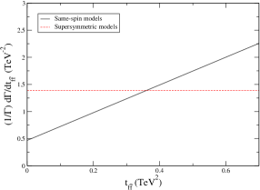
Figure 2: A plot of $\frac{1}{\Gamma}\frac{d\Gamma}{dt_{f\bar{f}}}$ as a function of $t_{f\bar{f}}$ for the reaction shown in Eq.(3). The same-spin scenario (solid-black) is contrasted with a supersymmetric scenario (dashed-red). The mass ratios are $M_{g^{\prime}}/M_{F}=2$ and $M_{F}/M_{\gamma^{\prime}}=5$. The only feature to note is simply the linear dependence of the same-spin scenario given by Eq.(3.1)

There is no parametric suppression of the slope as the coefficient of $t_{f\bar{f}}$ is of the same order as the constant term. However, a kinematical suppression is still present and when $M_{Q}^{2}/M_{\gamma^{\prime}}^{2}=2$ the slope vanishes. The origin of this suppression is simple: when $M_{Q}^{2}/M_{\gamma^{\prime}}^{2}=2$, the vector-boson $\gamma^{\prime}$ is an equal mixture of the transverse and longitudinal components and spin conservation does not choose any preferred alignment for the outgoing $f-\bar{f}$ pair. The sign of the slope can therefore provide additional kinematical information. As we shall see in the next section, it may, in fact, help determine the spin of $g^{\prime}$ and $\gamma^{\prime}$ as well.

To conclude, in the absence of any kinematical suppression such as $M_{Q}^{2}/M_{\gamma^{\prime}}^{2}\sim 2$, angular correlations are very pronounced and a histogram of the events should readily discover the linear dependence of $d\Gamma/dt_{f\bar{f}}$ on $t_{f\bar{f}}$.

3.2 Nearly Degenerate Spectrum, $\Delta M\ll\lambda v$

If the splitting between the diagonal elements of the mass matrix is very small $\Delta M\ll\lambda v$ the phase difference $\varphi$ between the diagonal elements is important. While the expression for the amplitude can be easily computed for a general phase, it is more illuminating to consider the two extreme cases $\varphi=0$ and $\varphi=\pi$.

When $\varphi=0$, mixing is maximal as we saw in the previous section. The interaction of $F_{1}^{\prime}$ with the SM is almost purely vector-like and that of $F_{2}^{\prime}$ is almost purely axial as seen from Eq.(8).

The mass splitting between the two states $F_{1}^{\prime}$ and $F_{2}^{\prime}$ is approximately $2\lambda v$. If the splitting is larger than the decay width of $F_{1}^{\prime}$ and $F_{2}^{\prime}$ then the interference between the two diagrams in Eq.(8) can be neglected and the NWA is justified. Using the NWA we find (to leading order in $\Delta M/\lambda v$),

$$\alpha = \frac{1}{2}\left(2M_{g^{\prime}}^{2}+\overline{M}^{2}\right)\left(\overline{M}^{2}+2M_{\gamma^{\prime}}^{2}\right)~{}t_{f\bar{f}}^{(edge)}$$

$$\beta = \left(2M_{g^{\prime}}^{2}-\overline{M}^{2}\right)\left(\overline{M}^{2}-2M_{\gamma^{\prime}}^{2}\right)~{}\left(\frac{\Delta M}{\lambda v}\right)^{2}.$$ (13)

This expression is very similar to the one we found in the previous case only that the coefficient of $t_{f\bar{f}}$ is subdominant to the constant piece and comes only at second order in the small parameter $\Delta M/\lambda v$. Angular correlations are therefore suppressed and vanish altogether in the degenerate limit. The reason for this is simple: both interaction vertices in Eq.(3) must be at least partially chiral to have any angular correlations [18].

A very rough lower bound on the number of events needed to determine that a non-zero slope is statistically significant is simply,

$$N\gtrsim\frac{1}{(\Delta M/\lambda v)^{4}}$$ (14)

Even when the suppression is only moderate, $\Delta M/\lambda v\sim 1/10$, the number of events required becomes exceedingly large.

On the other hand, when $\varphi=\pi$ as in UED, the mixing is minimal and the amplitude is the same as in the non-degenerate case, Eq.(3.1). Therefore, UED predicts that angular correlations are present between the $f-\bar{f}$ pair.

In an interesting recent paper, the authors of [16] claim that failure to observe angular correlations between the $f-\bar{f}$ pair establishes the existence of the gluino (albeit indirectly). The above discussion shows that this need not be the case. If the spectrum is non-degenerate, the correlations may simply be kinematically suppressed (when $M_{Q}^{2}\sim 2M_{\gamma^{\prime},Z^{\prime}}^{2}$). This possibility may be ruled-out by a proper measurement of the spectrum. If the spectrum is nearly degenerate, the phase $\varphi$ plays an important role. In this case, the mixing between the mass eigenstates, given by Eq.(5), is approximately,

$$\tan\theta=\frac{\lambda v\cos\left(\varphi/2\right)}{\Delta M+\sqrt{\Delta M^{2}+(\lambda v)^{2}\cos^{2}(\varphi/2)}}\quad\rightarrow\quad 1+\frac{\Delta M}{\lambda v\cos(\varphi/2)}$$ (15)

which is large in general. Only when $\varphi\rightarrow\pi$ does this expansion break down and mixing is diminished. Therefore, as we saw above, we expect the angular correlations to be suppressed by $\Delta M/\lambda v\cos(\varphi/2)$. Failing to observe angular correlation is therefore not necessarily an indication that the underlying model is SUSY. However, it is sufficient to rule-out the UED model which predicts $\varphi=\pi$.

3.3 Dilepton Correlations and the $Z^{\prime}$ Vertex

In the discussion above we examined the angular correlations between the SM fermions $f-\bar{f}$. Undoubtedly, the measurement of such correlations in the leptonic sector is considerably less challenging than the quark sector. One possible decay involving leptons is $Z^{\prime}\rightarrow\ell^{+}~{}\ell^{-}~{}\gamma^{\prime}$ through an intermediate heavy lepton. One may then question our initial choice for the coupling of the partners to the SM fields, Eq.(1). For example, a heavy $Z^{\prime}\sim W_{3}^{\prime}$ is likely to mix very little with a heavy $\gamma^{\prime}$ and therefore its interactions with the matter sector are strongly chiral to begin with. In this case, no amount of mixing between the mass eigenstates can change the chiral structure of the interactions.

Nonetheless, the analysis above is still relevant since as we argued before, the chirality of only one vertex is insufficient to guarantee spin effects in cascade decays. One must show that the other vertices are at least partially chiral to ascertain the existence of angular correlations.

One may also argue that the mixing between the lepton partners is always suppressed since the Yukawa couplings are small. In this paper we make no attempt at any general statements of this kind and only remark that in any model in which this is true, angular correlations between the outgoing $\ell^{-}\ell^{+}$ pair are indeed present.

4 Determining the Spin of $g^{\prime}$ and $Z^{\prime}/\gamma^{\prime}$

In cases where angular correlations are present, one can obtain more information than just the spin of the intermediate particle. It may even be possible to determine the spin of all the particles in a cascade decay.

In Table 1 we present the slope, $\beta_{F_{1}^{\prime}}$ in Eq.(10), for different spin choices for the external particles $g^{\prime}$ and $\gamma^{\prime}$ (similar expressions hold for $\beta_{F_{2}^{\prime}}$). When the two external particles are scalars the slope is unambiguously negative. In contrast, when the gluon partner $g^{\prime}$ is a vector-boson and $\gamma^{\prime}$ is a scalar the slope is unambiguously positive. These are simple consequences of spin conservation. However, when $\gamma^{\prime}$ is a vector-boson, the sign of the slope depends on whether $\gamma^{\prime}$ is longitudinally dominated ($M_{Q}^{2}>2M_{\gamma^{\prime}}^{2}$) or transversally dominated ($M_{Q}^{2}<2M_{\gamma^{\prime}}^{2}$).

Knowledge of the slope together with a measurement of the ratio $M_{Q}/M_{\gamma^{\prime}}$ (possibly from kinematical edges) can determine the spin of the external particle up to a two fold ambiguity. For example, if we measure a positive slope and $M_{Q}^{2}/M_{\gamma^{\prime}}^{2}>2$ we can conclude that the gluon partner is a vector-boson, but we do not know whether $\gamma^{\prime}$ is a scalar or a vector-boson. On the other hand, if the slope is positive and $M_{Q}^{2}/M_{\gamma^{\prime}}^{2}>2$ we would have concluded that $\gamma^{\prime}$ is a scalar, but we would have an ambiguity left regarding the spin of the gluon partner.

Scenario	Slope $\beta$	Intercept $\alpha$
	$\left(2M_{g^{\prime}}^{2}-M_{Q}^{2}\right)\left(M_{Q}^{2}-2M_{\gamma^{\prime}}^{2}\right)$	$(M_{Q}^{4}+4M_{\gamma^{\prime}}^{2}M_{g^{\prime}}^{2})~{}t_{f\bar{f}}^{(edge)}$
	$-\left(M_{Q}^{2}-2M_{\gamma^{\prime}}^{2}\right)$	$M_{Q}^{2}~{}t_{f\bar{f}}^{(edge)}$
	$\left(2M_{g^{\prime}}^{2}-M_{Q}^{2}\right)$	$M_{Q}^{2}~{}t_{f\bar{f}}^{(edge)}$
	$-1$	$t_{f\bar{f}}^{(edge)}$

Table 1: If angular correlations exist between the outgoing $f-\bar{f}$ or dilepton pair, then the sign of the slope of the distribution (whether $\beta>0$ or $\beta<0$) may reveal the spin of the external particles as well as the intermediate one. In the first row we consider a scenario where the external particles are both vector-bosons. In the second row the incoming partner is a scalar whereas the outgoing partner is a vector-boson and so forth.

Long cascade decays such as the one presented in Fig. 3 may contain enough information to determine the spin of all the partners unambiguously. For example, suppose we measure the slope of the $f-\bar{f}$ pair to be negative with $M_{F^{\prime}}^{2}/M_{Z^{\prime}}^{2}<2$ and that of the dilepton pair, $\ell^{-}-\ell^{+}$, to be negative with $M_{L^{\prime}}^{2}/M_{\gamma^{\prime}}^{2}<2$ as well. Then, either all three partners, $g^{\prime}$, $Z^{\prime}$ and $\gamma^{\prime}$, are vector-bosons, or all three are scalars. Hence, with a single spin measurement of the $Z^{\prime}$, such as described in [10, 11, 12, 13, 18], we can lift this two-fold ambiguity and determine the spin of all the particles in the event.

There are of course other discrepancies between the different scenarios which can, in principle, help remove the degeneracies. For example, in the limit where $M_{F_{1}^{\prime}}\gg M_{\gamma^{\prime}}$, the diagram with a vector-boson $\gamma^{\prime}$ is longitudinally enhanced over the other possibilities. However, these are numerical differences that do not affect the overall shape and may be hard to measure in practice when cross-sections and branching ratios cannot be determined very accurately. We have tried to emphasize some robust features of the distributions which do not relay on very accurate determination of the shape.

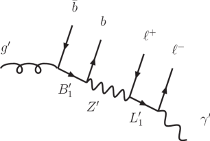
Figure 3: A possible long cascade decay in scenarios with same-spin partners. As explained in the text, a knowledge of the angular correlations between the $b-\bar{b}$ pair and dilepton $\ell^{-}-\ell^{+}$ may contain enough information to determine the spin of all the particles in the event, including $g^{\prime}$, $Z^{\prime}$ and $\gamma^{\prime}$.

5 Experimental Challenges and Strategy

The most daunting experimental difficulty for spin determination (and new physics in general) is SM background. We do not have much to say about it over what has already been discussed in the literature. Events with several final state leptons, hard jets and large missing energy are very rare in the SM and may prove to be strong signals of new physics. In what follows we will assume that some non-zero set of such events has been isolated and that the SM background is under control.

Once such a set is established one may begin to search for events where dilepton or $b-\bar{b}$ final states are present. At this stage it will be important to try and construct the event topology and identify a set of events with topologies such as discussed above. One may then look for angular correlations between dilepton or $b-\bar{b}$ pairs. However, there may be some ambiguity in the pairing (e.g. more then two leptons in an event or two leptons coming from different branches) which will result in a reduction of the signal due to combinatorics. As we showed in [18], this is not necessarily a disaster and may simply require more statistics to overcome the irreducible background.

An additional experimental aspect which may affect the signal is the collection of various cuts imposed on the outgoing particles. In particular $p_{T}$ and $\Delta R$ cuts will affect any invariant mass distribution such as the one described above. To investigate this point further we used the event generator HERWIG [20, 21] which we modified to include theories with same-spin partners [18]. In Fig. 4 we plot a histogram of the decay distribution as a function of $t_{f\bar{f}}$ for several experimental cuts. The comparison is made between SUSY and a general same-spin scenario. We require $p_{T}>100~{}\mathrm{GeV}$ on both outgoing fermions. We also apply different isolation cuts, $\Delta R>0.3$ and $\Delta R>0.7$, between the two fermions. While these cuts do not dramatically affect the distribution they do modify its lower end.

These results are presented here with the intent to illustrate the possible reshaping of such distributions due to experimental cuts. Clearly, many more experimental challenges have to be overcome before such a measurement is dubbed realistic. We emphasize that it is important to base such measurements on robust features of the distributions and not on tiny shape differences sensitive to a variety of experimental factors which may not even be sufficiently well-understood. Two such robust and important features to focus on are the existence of a non-zero slope and its sign.

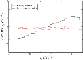
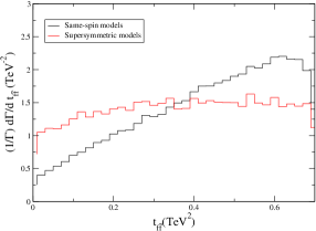
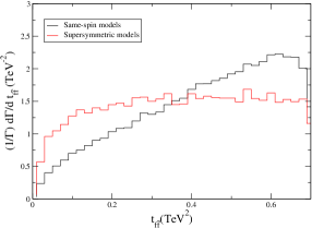
Figure 4: Plots of the decay distribution vs. $t_{f\bar{f}}=(p_{f}+p_{\bar{f}})^{2}$ for several experimental cuts. In the upper pane we present the Monte-Carlo results with no cuts. In the lower left pane a $p_{T}>100~{}\mathrm{GeV}$ cut was applied to both outgoing fermions together with $\Delta R>0.3$ isolation cut. In the lower right pane the isolation cut was increased to $\Delta R>0.7$. The mass parameters are such that $M_{g^{\prime}}/M_{F}=2$ and $M_{F}/M_{\gamma^{\prime}}=5$. The deterioration of the signal due to the cuts is visible at the lower end of the distribution.

6 Conclusions

If new particles are discovered at the LHC, it will be important to determine their spin. In light of the proliferation of new models in the recent decade, it is evident that Supersymmetry is not the only viable model for TeV scale physics. Many of the new models have, in fact, partners to the SM particles with the same spin as their SM counterparts. In this paper we investigated the general structure of such a sector and described the necessary conditions for spin effects to be observable.

When the fermionic partners of the left and right handed matter fields ($q_{L}$ and $u_{R}$ and $d_{R}$) have well-separated masses, angular correlations are always present regardless of the precise model (UED, Little Higgs and etc.). However, as the spectrum is squeezed and becomes more degenerate the mixing between the states is sensitive to an arbitrary phase in the mass matrix. In the UED model this phase is set by 5-d Lorentz invariance and the mixing remains small. In more general models this need not be the case and mixing can be very large. If such is the case, then spin information is washed out and consequently becomes harder to observe.

An observation of a non-zero slope will reveal the matter partners to be fermions. The sign of this slope may then be used to determine the spin of the external particles in the decay (such as the heavy gluon partner or other heavy vector-bosons). In certain cases it may even by possible to unambiguously infer the spin of all the particles involved in a cascade.

Acknowledgments : The Feynman diagrams in this paper were generated using Jaxodraw [22] and the plots were produced with the help of R [23] and Grace. The work of L.W. and I.Y. is supported by the National Science Foundation under Grant No. 0243680 and the Department of Energy under grant # DE-FG02-90ER40542. The work of C.K. is supported by the National Science Foundation under Grant NSF-PHY-0401513 and the Johns Hopkins Theoretical Interdisciplinary Physics and Astrophysics Center. Any opinions, findings, and conclusions or recommendations expressed in this material are those of the author(s) and do not necessarily reflect the views of the National Science Foundation.

Appendix A 3-site Deconstruction of UED

In this appendix we present a simple 3-site toy model for a scenario with same-spin SM partners. We illustrate the origin of the sign difference between the KK mass of the doublet $Q^{\prime}$ and that of the singlet $U^{\prime}$ (or $D^{\prime}$) in the UED model. We show that it is simply a consequence of the assumed 5-d Lorentz invariance of UED models. This serves to show that unless some special symmetry is enforced there is, in general, a phase difference between the masses, which is not necessarily $\varphi=\pi$ as in UED. Therefore, as we argued in the text, UED can be treated as a special limit of a generic 3-site model with same-spin partners.

We begin by writing a simple lagrangian involving 3 pairs of $SU(2)$ doublets, $\{Q_{iL}(x),Q_{iR}(x)\}$ with $i=1,2,3$,

$$\mathcal{L}_{Q}=\text{kinetic terms}+\frac{1}{a}\left(\overline{Q}_{1R},\overline{Q}_{2R},\overline{Q}_{3R}\right)\left(\begin{array}[]{ccc}0&1&-1\\ -1&0&1\\ 1&-1&0\end{array}\right)\left(\begin{array}[]{c}Q_{1L}\\ Q_{2L}\\ Q_{3L}\end{array}\right)+h.c.$$ (A-9)

This is simply a discrete version (with 3-sites) of an extra dimension compacted on a circle with inter-site separation $a$. The kinetic terms include the coupling to an $SU(2)$ gauge group on every site .

As it stands, this lagrangian has a $Z_{3}$ symmetry which reshuffles all three fields. This symmetry corresponds to the global $S_{1}$ symmetry, which is the conservation of 5-d momentum in the continuum limit. This $Z_{3}$ is broken down to $Z_{2}$ by orbifolding the geometry and identifying the first and third sites. This is most easily seen by going to an eigenstate basis of $Z_{2}$ and rewriting the lagrangian as,

$$\mathcal{L}_{Q}=\text{kinetic terms}+\frac{1}{a}\left(\overline{Q}_{R}^{(0)},\overline{Q}_{R}^{(cos)},\overline{Q}_{R}^{(sin)}\right)\left(\begin{array}[]{ccc}0&0&0\\ 0&0&-\sqrt{3}\\ 0&\sqrt{3}&0\end{array}\right)\left(\begin{array}[]{c}Q_{L}^{(0)}\\ Q_{L}^{(cos)}\\ Q_{L}^{(sin)}\end{array}\right)+h.c.$$ (A-16)

where we used the decomposition of the identity to write,

$$\left(\begin{array}[]{c}Q_{1L}\\ Q_{2L}\\ Q_{3L}\end{array}\right)=\frac{1}{\sqrt{3}}\left(\begin{array}[]{c}1\\ 1\\ 1\end{array}\right)Q_{L}^{(0)}+\frac{1}{\sqrt{6}}\left(\begin{array}[]{c}1\\ -2\\ 1\end{array}\right)Q_{L}^{(cos)}+\frac{1}{\sqrt{2}}\left(\begin{array}[]{c}1\\ 0\\ -1\end{array}\right)Q_{L}^{(sin)}$$ (A-17)

and similarly for the right-handed fermions. $Q^{(0)}$ is the zero mode and $Q^{(cos)}$ and $Q^{(sin)}$ correspond to the first KK level. These modes are even ($Q^{(0)}$, $Q^{(cos)}$) and odd ( $Q^{(sin)}$) under the $Z_{2}$ symmetry. Orbifolding the geometry we can project out the even (odd) states by choosing Dirichlet (Neumann) boundary conditions,

$$Q_{1}=Q_{3}\quad \rightarrow\quad Q^{(sin)}=0\quad\quad\text{Neumann b.c.}$$ (A-18)

$$Q_{2}=0\quad Q_{3}=-Q_{1}\quad \rightarrow\quad Q^{(0)}=Q^{(cos)}=0\quad\text{Dirichlet b.c.}$$ (A-19)

The SM contains a left handed doublet, but no right handed one so we should project out the odd modes for $Q_{L}$ and the even modes for $Q_{R}$. The resulting lagrangian is,

$$\mathcal{L}_{Q}=\text{kinetic terms}+m\overline{Q}_{R}^{(sin)}Q_{L}^{(cos)}+h.c.$$ (A-20)

where $m=\sqrt{3}/a$. Doing the same exercise with the singlet fields $U$ or $D$, we would have to choose the opposite boundary conditions. We see from Eq.(A-16) that we would pick the opposite sign for the singlets,

$$\mathcal{L}_{U}=\text{kinetic terms}-m\overline{U}_{R}^{(sin)}U_{L}^{(cos)}+h.c.$$ (A-21)

and similarly for the $D$. However, this sign depends on an arbitrary choice we made for the relative sign between the kinetic terms and the mass terms. 5-d Lorentz invariance fixes this sign to be the same for the doublets and singlets. This choice is the reason for the relative sign between the mass terms in Eq.(A-20) and Eq.(A-21). If no such symmetry is present, the phase is arbitrary and we have,

$$\mathcal{L}_{U}=\text{kinetic terms}+e^{i\phi}~{}m\overline{U}_{R}^{(sin)}U_{L}^{(cos)}+h.c.$$ (A-22)

Adding the contribution from the mixing with the Higgs mode we arrive at the mass matrix quoted in the text,

$$\mathcal{L}_{kk-mass}=\left(\begin{array}[]{cc}\overline{Q}_{R}^{(sin)},\overline{U}_{R}^{(cos)}\end{array}\right)\left(\begin{array}[]{cc}m&\lambda v\\ \lambda v&e^{i\phi}m\end{array}\right)\left(\begin{array}[]{c}Q_{L}^{(cos)}\\ U_{L}^{(sin)}\end{array}\right)$$ (A-23)

References

- [1] Thomas Appelquist, Hsin-Chia Cheng, and Bogdan A. Dobrescu. Bounds on universal extra dimensions. Phys. Rev., D64:035002, 2001.
- [2] Hsin-Chia Cheng, Konstantin T. Matchev, and Martin Schmaltz. Bosonic supersymmetry? getting fooled at the lhc. Phys. Rev., D66:056006, 2002.
- [3] N. Arkani-Hamed, A. G. Cohen, E. Katz, and A. E. Nelson. The littlest higgs. JHEP, 07:034, 2002.
- [4] N. Arkani-Hamed et al. The minimal moose for a little higgs. JHEP, 08:021, 2002.
- [5] Hsin-Chia Cheng and Ian Low. Tev symmetry and the little hierarchy problem. JHEP, 09:051, 2003.
- [6] Hsin-Chia Cheng and Ian Low. Little hierarchy, little higgses, and a little symmetry. JHEP, 08:061, 2004.
- [7] Ian Low. T parity and the littlest higgs. JHEP, 10:067, 2004.
- [8] Hsin-Chia Cheng, Ian Low, and Lian-Tao Wang. Top partners in little higgs theories with t-parity. 2005.
- [9] Hsin-Chia Cheng, Jesse Thaler, and Lian-Tao Wang. Little m-theory. JHEP, 09:003, 2006.
- [10] A. J. Barr. Using lepton charge asymmetry to investigate the spin of supersymmetric particles at the lhc. Phys. Lett., B596:205–212, 2004.
- [11] Marco Battaglia, AseshKrishna Datta, Albert De Roeck, Kyoungchul Kong, and Konstantin T. Matchev. Contrasting supersymmetry and universal extra dimensions at the clic multi-tev e+ e- collider. JHEP, 07:033, 2005.
- [12] Jennifer M. Smillie and Bryan R. Webber. Distinguishing spins in supersymmetric and universal extra dimension models at the large hadron collider. JHEP, 10:069, 2005.
- [13] AseshKrishna Datta, Kyoungchul Kong, and Konstantin T. Matchev. Discrimination of supersymmetry and universal extra dimensions at hadron colliders. Phys. Rev., D72:096006, 2005.
- [14] AseshKrishna Datta, Gordon L. Kane, and Manuel Toharia. Is it susy? 2005.
- [15] A. J. Barr. Measuring slepton spin at the lhc. JHEP, 02:042, 2006.
- [16] Alexandre Alves, Oscar Eboli, and Tilman Plehn. It’s a gluino. Phys. Rev., D74:095010, 2006.
- [17] Christiana Athanasiou, Christopher G. Lester, Jennifer M. Smillie, and Bryan R. Webber. Distinguishing spins in decay chains at the large hadron collider. JHEP, 08:055, 2006.
- [18] Lian-Tao Wang and Itay Yavin. Spin measurements in cascade decays at the lhc. 2006.
- [19] Jennifer M. Smillie. Spin correlations in decay chains involving w bosons. 2006.
- [20] G. Corcella et al. Herwig 6.5 release note. 2002.
- [21] Stefano Moretti, Kosuke Odagiri, Peter Richardson, Michael H. Seymour, and Bryan R. Webber. Implementation of supersymmetric processes in the herwig event generator. JHEP, 04:028, 2002.
- [22] D. Binosi and L. Theussl. Jaxodraw: A graphical user interface for drawing feynman diagrams. Comput. Phys. Commun., 161:76–86, 2004.
- [23] R Development Core Team. R: A Language and Environment for Statistical Computing. R Foundation for Statistical Computing, Vienna, Austria, 2006. ISBN 3-900051-07-0.