Soft gluon corrections to double transverse-spin asymmetries for small-$Q_{T}$ dilepton production
at RHIC and J-PARC

Abstract

We calculate the double transverse-spin asymmetries, ${\mathscr{A}_{TT}(Q_{T})}$, in transversely polarized Drell-Yan process at the transverse-momentum $Q_{T}$ of the produced lepton pair. We perform all-order resummation of the logarithmically enhanced contributions in the relevant Drell-Yan cross sections at small $Q_{T}$, which are due to multiple soft gluon emission in QCD, up to the next-to-leading logarithmic accuracy. The asymmetries ${\mathscr{A}_{TT}(Q_{T})}$ to be observed in polarized experiments at RHIC and J-PARC are studied numerically as a function of $Q_{T}$. We show that the effects of the soft gluon resummation to the polarized and unpolarized cross sections largely cancel in ${\mathscr{A}_{TT}(Q_{T})}$, but the significant corrections still remain and are crucial for making a reliable QCD prediction of ${\mathscr{A}_{TT}(Q_{T})}$. In particular, the soft gluon corrections enhance ${\mathscr{A}_{TT}(Q_{T})}$ considerably in the small $Q_{T}$ region compared with the asymmetry in the fixed-order $\alpha_{s}$ perturbation theory. We also derive a novel asymptotic formula which embodies those remarkable features of ${\mathscr{A}_{TT}(Q_{T})}$ at small $Q_{T}$ in a compact analytic form and is useful to extract the transversity $\delta q(x)$ from the experimental data.

1 Introduction

In recent years, a variety of experiments has been devoted to explore the spin-dependent phenomena in hard processes. Especially, experiments with transvesely polarized hadrons have opened a new window to study rich structure of perturbative/nonperturbative dynamics of QCD associated with the transverse spin [1]. One of the fundamental quantities which newly enter into play is the chiral-odd, twist-2 parton distribution, called the transversity $\delta q(x)$; it represents the distribution of transversly polarized quark inside transversly polarized nucleon, i.e, the partonic structure of the nucleon which is complementary to that associated with the other twist-2 distributions, such as the familiar density and helicity distributions $q(x)$ and $\Delta q(x)$. However, $\delta q(x)$ has not been well-known so far. This is because $\delta q(x)$ cannot be measured in inclusive DIS in contrast to $q(x)$ and $\Delta q(x)$; the chiral-odd nature requires a chirality flip, so that $\delta q(x)$ must be always accompanied with another chiral-odd function in physical observables. It is very recent that the first global fit of $\delta q(x)$ is given [2] using the semi-inclusive DIS data, in combination with the $e^{+}e^{-}$ data for the associated chiral-odd (Collins) fragmentation function.

Transversely polarized Drell-Yan (tDY) process, $p^{\uparrow}p^{\uparrow}\longrightarrow l^{+}l^{-}X$, is another promising process to access the transversity $\delta q(x)$. Based on QCD factorization, the spin-dependent cross section $\Delta_{T}d\sigma\equiv(d\sigma^{\uparrow\uparrow}-d\sigma^{\uparrow\downarrow})/2$ is given as a convolution, $\Delta_{T}d\sigma=\int dx_{1}dx_{2}\delta H(x_{1},x_{2};\mu_{F}^{2})$ $\Delta_{T}$$d\hat{\sigma}(x_{1}^{0}/x_{1},x_{2}^{0}/x_{2};Q^{2},\mu_{F}^{2}/Q^{2})$, where $Q$ is the dilepton mass, $\mu_{F}$ is the factorization scale,

$$\delta H(x_{1},x_{2};\mu_{F}^{2})=\sum_{q}e_{q}^{2}\left[\delta q(x_{1},\mu_{F}^{2})\delta\bar{q}(x_{2},\mu_{F}^{2})+\delta\bar{q}(x_{1},\mu_{F}^{2})\delta q(x_{2},\mu_{F}^{2})\right],$$ (1)

is the product of transversity distributions of the two nucleons, summed over the massless quark flavors $q$ with their charge squared $e_{q}^{2}$, and $\Delta_{T}d\hat{\sigma}=(d\hat{\sigma}^{\uparrow\uparrow}-d\hat{\sigma}^{\uparrow\downarrow})/2$ is the corresponding partonic cross section. $x_{1}^{0}=\sqrt{\tau}\ e^{y},x_{2}^{0}=\sqrt{\tau}\ e^{-y}$ are the relevant scaling variables, where $\tau=Q^{2}/S$, and $\sqrt{S}$ and $y$ are the total energy and dilepton’s rapidity in the nucleon-nucleon CM system. At the leading twist level, the gluon does not contribute to the transversely polarized, chiral-odd process, corresponding to helicity-flip by one unit. The unpolarized cross section, $d\sigma\equiv(d\sigma^{\uparrow\uparrow}+d\sigma^{\uparrow\downarrow})/2$, obeys factorization similar as $\Delta_{T}d\sigma$, in terms of $H(x_{1},x_{2};\mu_{F}^{2})$ that is given by (1) with $\delta q\rightarrow q$ and $\delta\bar{q}\rightarrow\bar{q}$, and additional functions involving the gluon distribution that comes in as higer-order $\alpha_{s}$ corrections. Therefore, the double-spin asymmetry in tDY, $A_{TT}\equiv\Delta_{T}d\sigma/d\sigma$, in principle provides clean information on the transversity $\delta q(x)$. At the leading order (LO) in QCD perturbation theory, $x_{1,2}^{0}$ coincide with the momentum fractions carried by the incident partons, e.g., $\Delta_{T}d\hat{\sigma}\propto\delta(x_{1}-x_{1}^{0})\delta(x_{2}-x_{2}^{0})$, so that [3, 1]

$$A_{TT}=\frac{\Delta_{T}d\sigma}{d\sigma}=\frac{1}{2}\cos(2\phi)\frac{\delta H(x_{1}^{0},x_{2}^{0};Q^{2})+\cdots}{H(x_{1}^{0},x_{2}^{0};Q^{2})+\cdots}\ ,$$ (2)

where $\phi$ denotes the azimuthal angle of one of the leptons with respect to the incoming nucleon’s spin axis, and the ellipses stand for the QCD corrections of NLO or higher. The $\cos(2\phi)$ dependence is characteristic of the spin-dependent cross section $\Delta_{T}d\sigma$ of tDY [3].

$A_{TT}$ to be observed in tDY at RHIC-Spin experiment was calculated by Martin et al. [4] including the NLO QCD corrections. The results are somewhat discouraging in that the corresponding $A_{TT}$ are at most a few percent [4].  The reason is twofold (see (2)): (i) tDY in $pp$ collisions probes the product of the quark transversity-distribution and the antiquark one as (1), and the latter is likely to be small; (ii) the rapid growth of the unpolarized sea-quark distributions in $H(x_{1}^{0},x_{2}^{0};Q^{2})$ is caused by the DGLAP evolution in the low-$x$ region that is typically probed at RHIC, $\sqrt{S}=200$ GeV, $Q\lesssim 10$ GeV, and $\sqrt{\tau}\lesssim 0.05$. Thus, small $A_{TT}$ at RHIC appears to be rather general conclusion (see also [5]).

We note that those previous NLO studies of $A_{TT}$ of (2) correspond to tDY with the transverse-momentum $Q_{T}$ of the produced lepton pair unobserved, and use the cross sections $\Delta_{T}d\sigma,d\sigma$ integrated over $Q_{T}$ in (2). However, in view of the fact that most of the lepton pairs are actually produced at small $Q_{T}$ in experiment, it is important to examine the double transverse-spin asymmetries at a measured $Q_{T}$, in particular its behavior for small $Q_{T}$. This is defined similarly as (2) using the “$Q_{T}$-differential” cross sections, and we denote it as ${\mathscr{A}_{TT}(Q_{T})}$ distinguishing from the conventional $Q_{T}$-independent $A_{TT}$. In fact, participation of the new scale $Q_{T}(\ll Q)$ causes profound modifications of the relevant theoretical framework. For example, now the numerator and the denominator of ${\mathscr{A}_{TT}(Q_{T})}$ may involve the parton distributions associated with the scales $\sim Q_{T}$, such as $\delta H(x_{1}^{0},x_{2}^{0};Q_{T}^{2})$ and $H(x_{1}^{0},x_{2}^{0};Q_{T}^{2})$, respectively. For $H(x_{1}^{0},x_{2}^{0};Q_{T}^{2})$, the low-$x$ rise of the unpolarized sea-quark distributions, mentioned in (ii) above, is milder compared with $H(x_{1}^{0},x_{2}^{0};Q^{2})$. Thus, if the former components play dominant roles compared with the latter in the denominator of ${\mathscr{A}_{TT}(Q_{T})}$ by certain partonic mechanism, ${\mathscr{A}_{TT}(Q_{T})}$ for small $Q_{T}$ region at RHIC can be larger than $A_{TT}$; the necessary partonic mechanism is indeed provided as the large logarithmic contributions of the type $\ln(Q^{2}/Q_{T}^{2})$, which is another remarkable consequence of the new scale $Q_{T}$: the small transverse-momentum $Q_{T}$ of the final lepton pair is provided by the recoil from the emission of soft gluons which produces the large terms behaving as $\alpha_{s}^{n}\ln^{m}(Q^{2}/Q_{T}^{2})/Q_{T}^{2}~{}(m=0,1,\ldots,2n-1)$ at each order of perturbation theory for the tDY cross sections. Actually, such enhanced “recoil logarithms” spoil the fixed-order perturbation theory, and have to be resummed to all orders in $\alpha_{s}$ to make a reliable prediction of the cross sections at small $Q_{T}$. Recently, we have worked out the corresponding “$Q_{T}$-resummation” for the tDY cross sections up to next-to-leading logarithmic (NLL) accuracy, which corresponds to summing up exactly the first three towers of logarithms, $\alpha_{s}^{n}\ln^{m}(Q^{2}/Q_{T}^{2})/Q_{T}^{2}$ with $m=2n-1,2n-2$ and $2n-3$, for all $n$ [6]. Utilizing this result, in the present paper, we develop QCD prediction for ${\mathscr{A}_{TT}(Q_{T})}$ as a function of $Q_{T}$.

We will demonstrate that the soft gluon corrections are significant so that ${\mathscr{A}_{TT}(Q_{T})}$ in the small $Q_{T}$ region is considerably large compared with the known value for $A_{TT}$.  In addition to ${\mathscr{A}_{TT}(Q_{T})}$ in tDY at RHIC, we calculate ${\mathscr{A}_{TT}(Q_{T})}$ to be observed at J-PARC when the polarized beam is realized [7]. The latter case is also interesting because the fixed target experiments at J-PARC probe the parton distributions in the medium $x$ region ($\sqrt{S}=10$ GeV, $Q\raisebox{-1.9919pt}{$\,\stackrel{{\scriptstyle>}}{{{\scriptstyle\sim}}}\,$}2$ GeV, and $\sqrt{\tau}\raisebox{-1.9919pt}{$\,\stackrel{{\scriptstyle>}}{{{\scriptstyle\sim}}}\,$}0.2$), and thus large asymmetries are expected even for the $Q_{T}$-independent $A_{TT}$ [9] (see (ii) above). We also find that ${\mathscr{A}_{TT}(Q_{T})}$ for $Q_{T}\approx 0$ deserves special attention from theoretical as well as experimental point of view, and derive a compact analytic formula for $\mathscr{A}_{TT}(Q_{T}\approx 0)$.

The paper is organized as follows. In Sec. 2, the $Q_{T}$-resummation formula for the tDY cross sections is introduced, and all ingredients necessary for calculating the $Q_{T}$-dependent asymmetries ${\mathscr{A}_{TT}(Q_{T})}$ including the NLL resummation contributions are explained. In Sec. 3, numerical results of ${\mathscr{A}_{TT}(Q_{T})}$ at RHIC and J-PARC are presented. Sec. 4 is devoted to the discussion of analytic formula of ${\mathscr{A}_{TT}(Q_{T})}$ at $Q_{T}\approx 0$ using the saddle-point method. Conclusions are given in Sec. 5.

2 Resummed cross section and asymmetry for tDY

Throughout the paper we employ the $\overline{\rm MS}$ factorization and renormalization scheme with the corresponding scales, $\mu_{F}$ and $\mu_{R}$. We first recall basic points of the fixed-order calculation of the spin-dependent, $Q_{T}$-differential cross sections of tDY [6]. In the lowest-order approximation via the Drell-Yan mechanism, the lepton pair is produced with vanishing $Q_{T}$, so that the corresponding partonic cross section is proportional to $\delta(Q_{T}^{2})$. The one-loop corrections to the partonic cross section involve the virtual gluon corrections, and the real gluon emission contributions, $q+\bar{q}\to l+\bar{l}+g$; in the latter case, the finite $Q_{T}$ of the lepton pair is provided by the recoil from the gluon radiation. Those have been calculated in the dimensional regularization [6], and the differential cross section of tDY is obtained as

$$\frac{\Delta_{T}d\sigma^{\rm FO}}{dQ^{2}dQ_{T}^{2}dyd\phi}=\cos{(2\phi)}\frac{\alpha^{2}}{3\,N_{c}\,S\,Q^{2}}\left[\Delta_{T}X\,(Q_{T}^{2}\,,\,Q^{2}\,,\,y)+\Delta_{T}Y\,(Q_{T}^{2}\,,\,Q^{2}\,,\,y)\right],$$ (3)

where $\Delta_{T}X$ and $\Delta_{T}Y$ are, respectively, expressed as the convolution of (1) with the corresponding partonic cross sections, see [6] for their explicit form in the $\overline{\rm MS}$ scheme: $\Delta_{T}X=\Delta_{T}X^{(0)}+\Delta_{T}X^{(1)}$ as the sum of ${\cal O}(\alpha_{s}^{0})$ and ${\cal O}(\alpha_{s}^{1})$ contributions, where $\alpha_{s}=\alpha_{s}(\mu_{R}^{2})$ with $\mu_{R}$ the renormalization scale, and $\Delta_{T}X^{(0)}=\delta H(x_{1}^{0}\,,\,x_{2}^{0}\,;\,\mu_{F}^{2})\ \delta(Q_{T}^{2})$. The partonic cross section associated with $\Delta_{T}X^{(1)}$ contains all terms that are singular as $Q_{T}\rightarrow 0$, behaving $Q_{T}^{-2}\times(\ln(Q^{2}/Q_{T}^{2})$ or $1)$ or $\delta(Q_{T}^{2})$, while the ${\cal O}(\alpha_{s})$ terms that are less singular than those in $\Delta_{T}X^{(1)}$ are included in the “finite” part $\Delta_{T}Y$. In (3), $\Delta_{T}X$ becomes very large as $\sim\alpha_{s}\ln(Q^{2}/Q_{T}^{2})/Q_{T}^{2}$ and $\sim\alpha_{s}/Q_{T}^{2}$ when $Q_{T}\ll Q$, representing the recoil effects from the emission of the soft and/or collinear gluon, and those terms have to be combined with the large contributions of similar nature that appear in each order of perturbation theory as $\alpha_{s}^{n}\ln^{2n-1}(Q^{2}/Q_{T}^{2})/Q_{T}^{2}$, $\alpha_{s}^{n}\ln^{2n-2}(Q^{2}/Q_{T}^{2})/Q_{T}^{2}$, and so on, from the multiple gluon emission.

The resummation of those logarithmically enhanced contributions to all orders has been worked out [6], in order to obtain a well-defined, finite prediction for the cross section. This is carried out by exponentiating the soft gluon effects in the impact parameter $b$ space, up to the NLL accuracy. As the result, $\Delta_{T}X$ of (3) is replaced by the corresponding NLL resummed component as $\Delta_{T}X\rightarrow\Delta_{T}X^{\rm NLL}$, with [6]

$$\Delta_{T}X^{\rm NLL}(Q_{T}^{2},Q^{2},y)=\sum_{i,j,k}e_{i}^{2}\int_{0}^{\infty}db\frac{b}{2}J_{0}(bQ_{T})e^{S(b,Q)}(C_{ij}\otimes f_{j})\left(x_{1}^{0},\frac{b_{0}^{2}}{b^{2}}\right)(C_{\bar{i}k}\otimes f_{k})\left(x_{2}^{0},\frac{b_{0}^{2}}{b^{2}}\right).$$ (4)

Here $J_{0}(bQ_{T})$ is a Bessel function for the two-dimensional Fourier transformation from the $b$ space to the $Q_{T}$ space, and $b_{0}=2e^{-\gamma_{E}}$ with $\gamma_{E}$ the Euler constant. The symbol $\otimes$ denotes convolution as $(C_{ij}\otimes f_{j})\ (x,\mu^{2})=\int_{x}^{1}\,(dz/z)\,C_{ij}(z,\alpha_{s}(\mu^{2}))\,f_{j}(x/z,\mu^{2})$. Note that the suffix $i,j,k$ can be either $q,\bar{q}$ including the flavor degrees of freedom, and we set $f_{q}(x,\mu^{2})\equiv\delta q(x,\mu^{2})$, $f_{\bar{q}}(x,\mu^{2})\equiv\delta\bar{q}(x,\mu^{2})$. The soft gluon effects are resummed into the Sudakov factor $e^{S(b,Q)}$ with

$$S(b,Q)=-\int_{b_{0}^{2}/b^{2}}^{Q^{2}}\frac{d\kappa^{2}}{\kappa^{2}}\left\{A_{q}(\alpha_{s}(\kappa^{2}))\ln\frac{Q^{2}}{\kappa^{2}}+B_{q}(\alpha_{s}(\kappa^{2}))\right\}.$$ (5)

The functions $A_{q}$, $B_{q}$ as well as the coefficient functions $C_{ij}$ are perturbatively calculable: $A_{q}(\alpha_{s})=\sum_{n=1}^{\infty}\left(\frac{\alpha_{s}}{2\pi}\right)^{n}A_{q}^{(n)}$, $B_{q}(\alpha_{s})=\sum_{n=1}^{\infty}\left(\frac{\alpha_{s}}{2\pi}\right)^{n}B_{q}^{(n)}$, and $C_{ij}(z,\alpha_{s})=\delta_{ij}\delta(1-z)+\sum_{n=1}^{\infty}\left(\frac{\alpha_{s}}{2\pi}\right)^{n}C_{ij}^{(n)}(z)$. At the NLL accuracy,

$$A_{q}^{(1)}=2C_{F},~{}~{}~{}A_{q}^{(2)}=2C_{F}\left\{\left(\frac{67}{18}-\frac{\pi^{2}}{6}\right)C_{G}-\frac{5}{9}N_{f}\right\},~{}~{}~{}B_{q}^{(1)}=-3C_{F},$$ (6)

where $C_{F}=(N_{c}^{2}-1)/(2N_{c})$, $C_{G}=N_{c}$, and $N_{f}$ is the number of QCD massless flavors, and

$$C_{ij}^{(1)}(z)=\delta_{ij}C_{F}\left(\frac{\pi^{2}}{2}-4\right)\delta(1-z)$$ (7)

are derived in [6]. The result (6) coincides with that obtained for other processes [10, 11], demonstrating that $\{A_{q}^{(1)},A_{q}^{(2)},B_{q}^{(1)}\}$ are universal (process-independent).  Substituting (6) and the running coupling constant $\alpha_{s}(\kappa^{2})$ at two-loop level, the $\kappa^{2}$ integral in (5) can be performed explicitly to the NLL accuracy, and the result can be systematically organized as (see also [13, 14])

$$S(b,Q) = \frac{1}{\alpha_{s}(\mu_{R}^{2})}h^{(0)}(\lambda)+h^{(1)}(\lambda)\ ,$$ (8)

where the first and second terms collect the LL and NLL contributions, respectively, as

$$h^{(0)}(\lambda) = \frac{A_{q}^{(1)}}{2\pi\beta_{0}^{2}}[\lambda+\ln(1-\lambda)],$$ (9)

$$h^{(1)}(\lambda) = \frac{A_{q}^{(1)}\beta_{1}}{2\pi\beta_{0}^{3}}\left[\frac{1}{2}\ln^{2}(1-\lambda)+\frac{\lambda+\ln(1-\lambda)}{1-\lambda}\right]+\frac{B_{q}^{(1)}}{2\pi\beta_{0}}\ln(1-\lambda)$$ (10)

$$-\frac{1}{4\pi^{2}\beta_{0}^{2}}\left[A_{q}^{(2)}-2\,\pi\beta_{0}A_{q}^{(1)}\ln\frac{Q^{2}}{\mu_{R}^{2}}\right]\left[\frac{\lambda}{1-\lambda}+\ln(1-\lambda)\right].$$

In these equations, $\beta_{0}\,,\,\beta_{1}$ are the first two coefficients of the QCD $\beta$ function given by $\beta_{0}=(11C_{G}-2N_{f})/(12\pi)$, $\beta_{1}=(17C_{G}^{2}-5C_{G}N_{f}-3C_{F}N_{f})/(24\pi^{2})$, and

$$\lambda=\beta_{0}\alpha_{s}(\mu_{R}^{2})\ln\frac{Q^{2}b^{2}}{b_{0}^{2}}\equiv\beta_{0}\alpha_{s}(\mu_{R}^{2})L\ .$$ (11)

In the $b$ space, $L=\ln(Q^{2}b^{2}/b_{0}^{2})$ plays the role of the large logarithmic expansion parameter with $b\sim 1/Q_{T}$, and $\lambda$ of (11) is formally considered as being of order unity in the resummed logarithmic expansion to the NLL in (8), where the neglected NNLL corrections are down by $\alpha_{s}(\mu_{R}^{2})$. Note that, expanding the above NLL formula (4) with (6)-(11) in powers of $\alpha_{s}(\mu_{R}^{2})$, the first three towers of logarithms, $\alpha_{s}^{n}\ln^{m}(Q^{2}/Q_{T}^{2})/Q_{T}^{2}$ with $m=2n-1,2n-2$ and $2n-3$, in the tDY differential cross section are fully reproduced for all $n$. Combining this expansion with the finite part $\Delta_{T}Y$ of (3), the result gives the tDY differential cross section which is exact up to ${\cal O}(\alpha_{s})$; thus we use the NLO parton distributions in the $\overline{\rm MS}$ scheme for $f_{j}(x,\mu^{2})$ in (4), as well as for those involved in $\Delta_{T}Y$.

We explain some further manipulations for our NLL formula; those were actually performed in [6], but were not described in detail. The integrand of (4) depends on the parton distributions at the scale $b_{0}/b$, according to the general formulation [15]. Taking the Mellin moments of $\Delta_{T}X^{\rm NLL}(Q_{T}^{2},Q^{2},y)$ with respect to the DY scaling variables $x_{1,2}^{0}$ at fixed $Q$,

$$\Delta_{T}X^{\rm NLL}_{N_{1},N_{2}}(Q_{T}^{2},Q^{2})\equiv\int_{0}^{1}dx_{1}^{0}\left(x_{1}^{0}\right)^{N_{1}-1}\int_{0}^{1}dx_{2}^{0}\left(x_{2}^{0}\right)^{N_{2}-1}\Delta_{T}X^{\rm NLL}(Q_{T}^{2},Q^{2},y),$$ (12)

the $b$-dependence of those parton distributions can be disentangled because the moments, $f_{i,N}(\mu^{2})\equiv\int_{0}^{1}dxx^{N-1}f_{i}(x,\mu^{2})$, obey the renormalization group (RG) evolution as $f_{i,N}(b_{0}^{2}/b^{2})$ $=\sum_{j}U_{ij,N}(b_{0}^{2}/b^{2},Q^{2})f_{j,N}(Q^{2})$, where $U_{ij,N}(\mu^{2},{\mu^{\prime}}^{2})$ are the NLO evolution operators for the transversity distributions which are expressed in terms of the corresponding LO and NLO anomalous dimensions [16, 17] and the two-loop running coupling constant. For (12) with (4) and the above RG evolution substituted, several “reorganization” of the relevant large-logarithmic expansion is necessary for its consistent evaluation over the entire range of $Q_{T}$, following the systematic procedure in [14] elaborated for unpolarized hadron collisions: exploiting the RG invariance, we have $C_{ij,N}(\alpha_{s}(b_{0}^{2}/b^{2}))=C_{ij,N}(\alpha_{s}(Q^{2}))e^{[\alpha_{s}(\mu_{R}^{2})C_{ij,N}^{(1)}/2\pi]\lambda/(1-\lambda)}$ to the corrections down by $\alpha_{s}(\mu_{R}^{2})$, for the $N$-th moment of the coefficient function of (7), so that we make the replacement $C_{ij,N}(\alpha_{s}(b_{0}^{2}/b^{2}))\rightarrow C_{ij,N}(\alpha_{s}(Q^{2}))=\delta_{ij}[1+(\alpha_{s}(Q^{2})C_{F}/4\pi)(\pi^{2}-8)]$, up to the corrections of NNLL level for (12). Similarly, performing the large-logarithmic expansion for explicit formula of the NLO evolution operator $U_{ij,N}(b_{0}^{2}/b^{2},Q^{2})$, we find

$$U_{ij,N}(b_{0}^{2}/b^{2},Q^{2})=\delta_{ij}e^{R_{N}(\lambda)},\;\;\;\;\;\;\;\;R_{N}(\lambda)\equiv\frac{\Delta_{T}P_{qq,N}}{2\pi\beta_{0}}\ln(1-\lambda),$$ (13)

up to the corrections down by $\alpha_{s}(\mu_{R}^{2})$ which correspond to the NNLL terms when substituted into (12), (4). Here $\Delta_{T}P_{qq,N}=-2C_{F}[\psi(N+1)+\gamma_{E}-3/4]$ is the $N$-th Mellin moment of the LO DGLAP splitting function for the transversity. As a result, (12) is expressed as

$$\Delta_{T}X^{\rm NLL}_{N_{1},N_{2}}(Q_{T}^{2},Q^{2}) =\left[1+\frac{\alpha_{s}(Q^{2})}{2\pi}C_{F}(\pi^{2}-8)\right]\delta H_{N_{1},N_{2}}(Q^{2})I_{N_{1},N_{2}}(Q_{T}^{2},Q^{2})\ ,$$ (14)

$$I_{N_{1},N_{2}}(Q_{T}^{2},Q^{2}) \equiv\int_{0}^{\infty}db\frac{b}{2}J_{0}(bQ_{T})e^{S(b,Q)+R_{N_{1}}(\lambda)+R_{N_{2}}(\lambda)}\ ,$$ (15)

where $\delta H_{N_{1},N_{2}}(Q^{2})$ is the double Mellin-moments of $\delta H(x_{1}^{0},x_{2}^{0};Q^{2})$ of (1), defined similarly as (12). The complete dependence on $b$ is included in the exponential factor $e^{S(b,Q)+R_{N_{1}}(\lambda)+R_{N_{2}}(\lambda)}$ through $L=\ln(Q^{2}b^{2}/b_{0}^{2})$, so that all-order resummation of the large logarithms $L$ and the associated $b$-integral in (15) are now accomplished at the partonic level.

We also mention some other “reorganization”, which is explained in [6] and is necessary in order to treat properly too short and long distance involved in the $b$ integration of (15): firstly, to treat too short distance $Qb\ll 1$, we make the replacement

$$L\rightarrow\tilde{L}=\ln(Q^{2}b^{2}/b_{0}^{2}+1)\ ,$$ (16)

in the definition (11) of $\lambda$, following [14]; note that the integrand of (15) depends on the large-logarithmic expansion parameter only through $\lambda$ (see (8)-(10), (13)). This replacement allows us to reduce the unjustified large logarithmic contributions for $Qb\ll 1$, due to $L\gg 1$, as $\tilde{L}\rightarrow 0$ and $e^{S(b,Q)+R_{N_{1}}(\lambda)+R_{N_{2}}(\lambda)}\rightarrow 1$, while $L$ and $\tilde{L}$ are equivalent to organize the soft gluon resummation at small $Q_{T}$ as $\tilde{L}=L+{\cal O}(1/(Qb)^{2})$ for $Qb\gg 1$. Secondly, the functions (9) and (10) in the Sudakov exponent (8) are singular when $\lambda=\beta_{0}\alpha_{s}(\mu_{R}^{2})\tilde{L}\rightarrow 1$, and this singular behavior is related to the presence of the Landau pole in the perturbative running coupling $\alpha_{s}(\kappa^{2})$ in QCD. To properly define the $b$ integration of (15) for the corresponding long-distance region, it is necessary to specify a prescription to deal with this singularity [13]: decomposing the Bessel function in (15) into the two Hankel functions as $J_{0}(bQ_{T})=(H_{0}^{(1)}(bQ_{T})+H_{0}^{(2)}(bQ_{T}))/2$, we deform the $b$-integration contour for these two terms into upper and lower half plane in the complex $b$ space, respectively, and obtain the two convergent integrals as $|b|\rightarrow\infty$. The new contour ${\cal C}$ is taken as: from $b=0$ to $b=b_{c}$ on the real axis, followed by the two branches, $b=b_{c}+e^{\pm i\theta}t$ with $t\in\{0,\infty\}$ and $0<\theta<\pi/4$; a constant $b_{c}$ is chosen as $0\leq b_{c}<b_{L}$, where $b=b_{L}$ gives the solution for $\lambda=1$. Note, this choice of contours is completely equivalent to the original contour, order-by-order in $\alpha_{s}(\mu_{R}^{2})$, when the corresponding formulae are expanded in powers of $\alpha_{s}$. Therefore, this contour deformation prescription provides us with a (formally) consistent definition of finite $b$-integral of (15) within a perturbative framework.

We now denote (14), with the replacement (16) and the new contour ${\cal C}$ in (15), as $\Delta_{T}\tilde{X}^{\rm NLL}_{N_{1},N_{2}}(Q_{T}^{2},Q^{2})$, and also denote the double inverse Mellin transform of $\Delta_{T}\tilde{X}^{\rm NLL}_{N_{1},N_{2}}(Q_{T}^{2},Q^{2})$, from $(N_{1},N_{2})$ space to $(x_{1}^{0},x_{2}^{0})$ space, as $\Delta_{T}\tilde{X}^{\rm NLL}(Q_{T}^{2},Q^{2},y)$. Defining (see (3))

$$\Delta_{T}\tilde{Y}(Q_{T}^{2},Q^{2},y)\equiv\Delta_{T}X(Q_{T}^{2},Q^{2},y)+\Delta_{T}Y(Q_{T}^{2},Q^{2},y)-\left.\Delta_{T}\tilde{X}^{\rm NLL}(Q_{T}^{2},Q^{2},y)\right|_{\rm FO}\ ,$$ (17)

where $\Delta_{T}\tilde{X}^{\rm NLL}(Q_{T}^{2},Q^{2},y)|_{\rm FO}$ denotes the terms resulting from the expansion of the resummed expression up to the fixed-order $\alpha_{s}(\mu_{R}^{2})$, we obtain the final form of our differential cross section for tDY with the soft gluon resummation as [6]

$$\frac{\Delta_{T}d\sigma}{dQ^{2}dQ_{T}^{2}dyd\phi}=\cos(2\phi)\frac{\alpha^{2}}{3\,N_{c}\,S\,Q^{2}}\biggl{[}\Delta_{T}\tilde{X}^{\rm NLL}(Q_{T}^{2},Q^{2},y)+\Delta_{T}\tilde{Y}(Q_{T}^{2},Q^{2},y)\biggr{]}.$$ (18)

From the derivation explained above, the expansion of this cross section in powers of $\alpha_{s}(\mu_{R}^{2})$ fully reproduces the first three towers of logarithms, $\alpha_{s}^{n}\ln^{m}(Q^{2}/Q_{T}^{2})/Q_{T}^{2}$ with $m=2n-1,2n-2$ and $2n-3$, associated with the soft-gluon emission for small $Q_{T}$ ($\ll Q$), and also coincides exactly with the fixed-order result (3) to ${\cal O}(\alpha_{s})$. Therefore, this formula (18) avoids any double counting over the entire range of $Q_{T}$. Note that $\Delta_{T}\tilde{Y}(Q_{T}^{2},Q^{2},y)$ of (17) corresponds to the “modified finite component” in our resummation framework: because the first and the third terms in the RHS of (17) cancel with each other for $Q_{T}\ll Q$, $\Delta_{T}\tilde{Y}(Q_{T}^{2},Q^{2},y)$ is less singular as $Q_{T}\rightarrow 0$ than $Q_{T}^{-2}\times(\ln(Q^{2}/Q_{T}^{2})$ or $1)$ or $\delta(Q_{T}^{2})$, see the discussion below (3). Combined with $\Delta_{T}X^{(0)}\propto\delta(Q_{T}^{2})$, this also implies that $\Delta_{T}\tilde{Y}(Q_{T}^{2},Q^{2},y)$ is of order $\alpha_{s}(\mu_{R}^{2})$. In fact, (17) coincides exactly with $\Delta_{T}Y(Q_{T}^{2},Q^{2},y)$ if (16) is not performed.

Because of this “regular” behavior of $\Delta_{T}\tilde{Y}(Q_{T}^{2},Q^{2},y)$ as $Q_{T}\rightarrow 0$, we may consider (17) as the definition for the region where $Q_{T}>0$; in this case, the first two terms correspond to (3) for $Q_{T}>0$, i.e.,

$$\frac{\Delta_{T}d\sigma^{\rm LO}}{dQ^{2}dQ_{T}^{2}dyd\phi}=\cos{(2\phi)}\frac{\alpha^{2}}{3\,N_{c}\,S\,Q^{2}}\left[\Delta_{T}\left.X^{(1)}\,(Q_{T}^{2},Q^{2},y)\right|_{Q_{T}^{2}>0}+\Delta_{T}Y\,(Q_{T}^{2},Q^{2},y)\right],$$ (19)

which gives the formula for the LO QCD prediction of tDY at the large-$Q_{T}$ region. Therefore, our formula (18) is actually the NLL resummed part, with the contributions to ${\cal O}(\alpha_{s})$ (the third term of (17)) subtracted, plus the LO cross section; we refer to (18) as the “NLL+LO” prediction, which gives the well-defined tDY differential cross section in the $\overline{\rm MS}$ scheme over the entire range of $Q_{T}$. It is straightforward to see that the integral of (18) over $Q_{T}$ reproduces that of (3) exactly, because $\tilde{L}=0$ at $b=0$ (see also [14]).

We can extend the above results to unpolarized DY by mostly trivial substitutions to switch from spin-dependent quantities to spin-averaged ones, e.g., by removing “$\Delta_{T}$” and making the replacement, $\delta H(x_{1},x_{2};\mu^{2})\rightarrow H(x_{1},x_{2};\mu^{2})$, $\cos(2\phi)\alpha^{2}/(3N_{c}SQ^{2})$ $\rightarrow 2\alpha^{2}/(3N_{c}SQ^{2})$, etc., in the above relevant formulae. The explicit form of the spin-averaged quantities, such as $X(Q_{T}^{2},Q^{2},y)$, $Y(Q_{T}^{2},Q^{2},y)$, as well as those corresponding to the coefficient functions $C_{ij}(z,\alpha_{s})$ in (4), can be obtained from the results in [15, 18]. A different point from the polarized case is that now the gluon distribution $f_{g}(x,\mu^{2})\equiv g(x,\mu^{2})$ participates, so that the suffix $i,j$ of the “spin-averaged $C_{ij}(z,\alpha_{s})$” can be “$g$” as well as “$q,\bar{q}$”. This also implies that $\Delta_{T}P_{qq,N}$ appearing in (13) has to be replaced by the Mellin moment of the LO DGLAP splitting functions for the unpolarized case, which involve the mixing of gluon, and the “new $U_{ij,N}(b_{0}^{2}/b^{2},Q^{2})$” represent the corresponding “evolution matrix” that was discussed in [14, 13]. On the other hand, the formulae (8)-(10) of the Sudakov exponent hold also for the unpolarized case, reflecting that the coefficients (6) relevant at the NLL level are universal [11, 12, 13, 14]. We list explicit form of the relevant formulae for the unpolarized cross sections in Appendix.

Taking the ratio of (18) to the corresponding NLL+LO prediction for unpolarized differential cross section, we obtain the double transverse-spin asymmetry in tDY, for transverse-momentum $Q_{T}$, invariant-mass $Q$, and rapidity $y$ of the produced lepton pair, and azimuthal angle $\phi$ of one of the leptons, as

$${\mathscr{A}_{TT}(Q_{T})}=\frac{1}{2}\cos(2\phi)\frac{\Delta_{T}\tilde{X}^{\rm NLL}(Q_{T}^{2},Q^{2},y)+\Delta_{T}\tilde{Y}(Q_{T}^{2},Q^{2},y)}{\tilde{X}^{\rm NLL}(Q_{T}^{2},Q^{2},y)+\tilde{Y}(Q_{T}^{2},Q^{2},y)}.$$ (20)

To the fixed-order $\alpha_{s}$ without the soft gluon resummation, (20) reduces to the LO prediction of the asymmetry for $Q_{T}>0$,

$$\mathscr{A}_{TT}^{\rm LO}(Q_{T})=\frac{1}{2}\cos(2\phi)\frac{\left.\Delta_{T}X^{(1)}(Q_{T}^{2},Q^{2},y)\right|_{Q_{T}^{2}>0}+\Delta_{T}Y(Q_{T}^{2},Q^{2},y)}{\left.X^{(1)}(Q_{T}^{2},Q^{2},y)\right|_{Q_{T}^{2}>0}+Y(Q_{T}^{2},Q^{2},y)},$$ (21)

as the ratio of (19) to the corresponding unpolarized cross section.

3 The asymmetries ${\mathscr{A}_{TT}(Q_{T})}$ at RHIC and J-PARC

We evaluate the asymmetries, derived in the last section, as a function of $Q_{T}$. We use the similar parton distributions as in the previous NLO studies [4] of $Q_{T}$-independent $A_{TT}$ of (2): for the transversity $\delta q(x,Q^{2})$ participating in the numerator of the asymmetries, we use a model of the NLO transversity distributions, which obey the corresponding NLO DGLAP evolution equation and are assumed to saturate the Soffer bound [19] as $\delta q(x,\mu^{2}_{0})=[q(x,\mu^{2}_{0})+\Delta q(x,\mu^{2}_{0})]/2$ at a low input scale $\mu_{0}\simeq 0.6$ GeV using the NLO GRV98 [20] and GRSV2000 (“standard scenario”) [21] distributions $q(x,\mu_{0}^{2})$ and $\Delta q(x,\mu^{2}_{0})$, respectively. The NLO GRV98 distributions $q(x,Q^{2}),g(x,Q^{2})$ are also used for calculating the unpolarized cross sections in the denominator of the asymmetries.

It is known that the $Q_{T}$-spectrum of DY lepton pair is affected by another nonperturbative effects, which become important for small $Q_{T}$ region [15]: we have obtained the well-defined tDY cross sections and asymmetries that are free from any singularities, with a consistent definition of the integration in (15) over the whole $b$ region. However, the integrand of (15) involving purely perturbative quantities is not accurate for extremely large $|b|$ region in QCD, and the corresponding long-distance behavior has to be complemented by the relevant nonperturbative effects. Formally those nonperturbative effects play role to compensate the ambiguity that the prescription for the $b$ integration in (15) to avoid the singularity in the Sudakov exponent $S(b,Q)$ of (8)-(10) is actually not unique (see [15]). Therefore, following [15, 13, 14], we make the replacement in (15) as

$$e^{S(b,Q)}\rightarrow e^{S(b,Q)-g_{NP}b^{2}},$$ (22)

with a nonperturbative parameter $g_{NP}$. Because exactly the same Sudakov factor $e^{S(b,Q)}$ participates in the corresponding formula for the unpolarized case as noted above (20), we perform the replacement (22) with the same nonperturbative parameter $g_{NP}$ in the NLL+LO unpolarized differential cross section contributing to the denominator of (20). This may be interpreted as assuming the same “intrinsic transverse momentum” of partons inside nucleon for both polarized and unpolarized cases, corresponding to the Gaussian smearing factor of (22). We use $g_{NP}\simeq 0.5$ GeV², suggested by the study of the $Q_{T}$-spectrum in unpolarized case [22].

For all the following numerical evaluations, we choose $\phi=0$ for the azimuthal angle of one lepton, $\mu_{F}=\mu_{R}=Q$ for the factorization and renormalization scales and $b_{c}=0$, $\theta=\frac{7}{32}\pi$ for the integration contour ${\cal C}$ explained below (16).

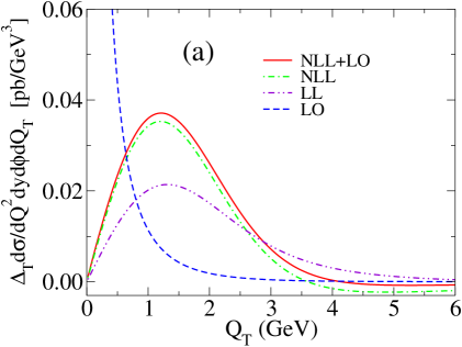
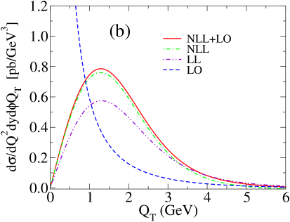
Figure 1: The spin-dependent and spin-averaged differential cross sections for tDY: (a) $\Delta_{T}d\sigma/dQ^{2}dQ_{T}dyd\phi$ and (b) $d\sigma/dQ^{2}dQ_{T}dyd\phi$, as a function of $Q_{T}$ at RHIC kinematics, $\sqrt{S}=200$ GeV, $Q=5$ GeV, $y=2$ and $\phi=0$, with $g_{NP}=0.5$ GeV².

First of all, we present the transvserse-momentum $Q_{T}$-spectrum of the DY lepton pair for $\sqrt{S}=200$ GeV, $Q=5$ GeV, and $y=2$, which correspond to the detection of dileptons with the PHENIX detector at RHIC. The solid curve in Fig. 1(a) shows the NLL+LO differential cross section (18) for tDY, multiplied by $2Q_{T}$, with $g_{NP}=0.5$ GeV² for (22). We also show the contribution from the NLL resummed component $\Delta_{T}\tilde{X}^{\rm NLL}$ in (18) by the dot-dashed curve, and the LO result using (19) by the dashed curve. Fig. 1(b) is same as Fig. 1(a) but for the unpolarized differential cross sections. The LO results become large and diverge as $Q_{T}\rightarrow 0$, while the NLL+LO results are finite and well-behaved over all regions of $Q_{T}$. The soft gluon resummation gives dominant contribution around the peak of the solid curve, i.e., at intermediate $Q_{T}$ as well as small $Q_{T}$. To demonstrate the resummation effects in detail, the two-dot-dashed curves in Figs. 1(a), (b) show the LL result which is obtained from the corresponding NLL result (dot-dashed curve) by omitting the contributions corresponding to the NLL level, i.e., $h^{(1)}(\lambda)$, $R_{N_{1}}(\lambda)$, $R_{N_{2}}(\lambda)$ in (15) and $\alpha_{s}(Q^{2})C_{F}(\pi^{2}-8)/2\pi$ in (14) for the polarized case (see (8) and the discussion below (11)), and similarly for the unpolarized case. The LL contributions are sufficient for obtaining the finite cross section, causing considerable suppression in the small $Q_{T}$ region. On the other hand, it is remarkable that the contributions at the NLL level provide significant enhancement from the LL result, around the peak region for both polarized and unpolarized cases, and the effect is more pronounced for the former. Among the relevant NLL contributions, the “universal” term $h^{(1)}(\lambda)$ produces similar (enhancement) effect for both (a) and (b) of Fig. 1, while the other NLL contributions, associated with the evolution operators and the ${\cal O}(\alpha_{s}(Q^{2}))$ coefficient functions (see e.g. (13), (14)), give different effects to the polarized and unpolarized cases.

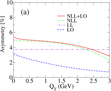
Figure 2: The asymmetries ${\mathscr{A}_{TT}(Q_{T})}$ at RHIC kinematics, $\sqrt{S}=200$ GeV, $Q=5$ GeV, $y=2$ and $\phi=0$: (a) ${\mathscr{A}_{TT}(Q_{T})}$ obtained from each curve in Fig. 1. (b) The NLL+LO ${\mathscr{A}_{TT}(Q_{T})}$ of (20) with (22) using various values for $g_{NP}$.

Fig. 2(a) shows the double transverse-spin asymmetries in the small $Q_{T}$ region for tDY at RHIC, obtained as the ratio of the results in Fig. 1(a) to the corresponding results in Fig. 1(b) for respective lines, so that the solid curve gives the NLL+LO result (20), the dot-dashed curve shows the NLL result,

$$\mathscr{A}_{TT}^{\rm NLL}(Q_{T})=\frac{1}{2}\cos(2\phi)\frac{\Delta_{T}\tilde{X}^{\rm NLL}(Q_{T}^{2},Q^{2},y)}{\tilde{X}^{\rm NLL}(Q_{T}^{2},Q^{2},y)}\ ,$$ (23)

and the dashed curve shows the LO result (21). The NLL+LO result is almost flat for $Q_{T}\rightarrow 0$ as well as around the peak region of the NLL+LO cross section in Fig. 1. This flat behavior is dominated by the NLL resummed components, and reflects the fact that the soft gluon emission effects resummed into the Sudakov factor $e^{S(b,Q)}$ with (8) are universal to the NLL accuracy between the numarator and denominator of (20). Slight increase of the solid line for $Q_{T}\rightarrow 0$ is due to the terms $\propto\ln(Q^{2}/Q_{T}^{2})$ contained in the “regular components” $\Delta_{T}\tilde{Y}$ and $\tilde{Y}$ in (20) (see (17)), but such weak singularities which show up only at very small $Q_{T}$ will be irrelevant for most practical purposes. The LO result, obtained as the ratio of the two LO curves divergent as $Q_{T}\rightarrow 0$ in Figs. 1(a) and (b), gives the finite asymmetry for $Q_{T}>0$, but it does not have the flat behavior, i.e., decreases for increasing $Q_{T}$, and is much smaller than the NLL+LO result. On the other hand, we note that the LL result, retaining only the resummmed components corresponding to the LL level, is given by (see (14), (15))

$$\mathscr{A}_{TT}^{\rm LL}(Q_{T})=\frac{1}{2}\cos(2\phi)\frac{\delta H(x_{1}^{0},x_{2}^{0};Q^{2})}{H(x_{1}^{0},x_{2}^{0};Q^{2})}\approx A_{TT}\ ,$$ (24)

which is independent of $Q_{T}$, because the $Q_{T}$-dependent factor (15) with $S(b,Q)+R_{N_{1}}(\lambda)+R_{N_{2}}(\lambda)\rightarrow h^{(0)}(\lambda)/\alpha_{s}(Q^{2})$ is common for both polarized and unpolarized cases. Namely the LL resummation effects cancel exactly between the numerator and the denominator in the asymmetry (24). As indicated in (24), the resulting value shown by the two-dot-dashed curve in Fig. 2(a) coincides with the $Q_{T}$-independent asymmetry (2) up to the NLO QCD corrections; note that $A_{TT}=4.0$% including the NLO corrections similarly as [4] (see Table 1 below). However, we recognize that the soft-gluon resummation contributions at the NLL level enhances the asymmetry at the small $Q_{T}$-region significantly, compared with the LL or fixed-order result. This is caused by the enhancement of the cross sections in Fig. 1 discussed above, due to the universal $h^{(1)}(\lambda)$ term and the other spin-dependent contributions. In particular, the evolution operators like (13) in the latter contributions allow the participation of the parton distributions at the scale $b_{0}/b\sim Q_{T}$, and the components associated with those parton distributions indeed play dominant roles due to the mechanism embodied by the Sudakov factor $e^{S(b,Q)}$ of (15). Combined with the different $x$-dependence between the transversity and density distributions as noted in (ii) above, the resulting enhancement arises differently between (a) and (b) in Fig. 1, and enhances the asymmetry as in Fig. 2(a).

In Fig. 2(b) we show the NLL+LO asymmetries ${\mathscr{A}_{TT}(Q_{T})}$ of (20), with (22) using various values of $g_{NP}$. Here the solid curve is the same as the solid curve in Fig. 2(a), using $g_{NP}=0.5$ GeV². The result demonstrates that our NLL+LO asymmetry in the relevant small-$Q_{T}$ region is almost independent of the value of $g_{NP}$ in the range $g_{NP}=0.3$-0.8 GeV². Although, at RHIC kinematics, the $Q_{T}$-spectrum from the spin-dependent cross section (18) with (22) receives a sizable smearing effect in the relevant small-$Q_{T}$ region [6], the corresponding $g_{NP}$-dependence is canceled by the similar dependence of the unpolarized cross section in the asymmetry (20). In our framework, such cancellation of the $g_{NP}$-dependence between the numerator and the denominator of (20) is observed for all relevant kinematics of our interest at RHIC, and also at J-PARC discussed below. However, we mention that too small value of $g_{NP}$ is useless in practice: the Gaussian smearing factor of (22) for $g_{NP}=0.1$ GeV² is insufficient to suppress sensitivity to the extremely large $|b|$ region in (15), so that the $b$ integration receives the “inaccurate” long-distance perturbative contributions considerably at small $Q_{T}$, which lead to unstable numerical behavior for $Q_{T}\raisebox{-1.9919pt}{$\,\stackrel{{\scriptstyle<}}{{{\scriptstyle\sim}}}\,$}1$ GeV. For all the following calculations, we use $g_{NP}=0.5$ GeV².

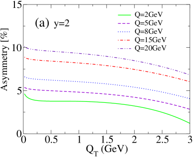
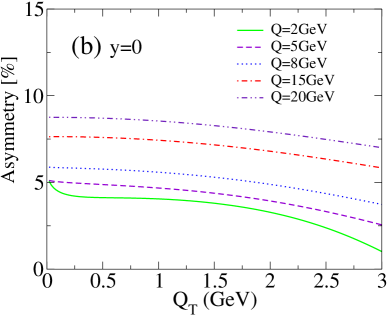
Figure 3: The NLL+LO ${\mathscr{A}_{TT}(Q_{T})}$ of (20) with (22) using $g_{NP}=0.5$ GeV² at RHIC kinematics, $\sqrt{S}=200$ GeV, $\phi=0$ with $y=2$ and $y=0$ for (a) and (b), respectively.

Fig. 3 shows the NLL+LO asymmetries ${\mathscr{A}_{TT}(Q_{T})}$ of (20) at RHIC kinematics, $\sqrt{S}=200$ GeV and various values of the dilepton invariant mass $Q$, using $y=2$ and $y=0$ for (a) and (b), respectively; the dashed curve in (a) is the same as the solid curve in Figs. 2(a), (b). For all cases in Fig. 3, we observe the typical flat behavior of ${\mathscr{A}_{TT}(Q_{T})}$ in the small $Q_{T}$ region, similarly as Fig. 2. On the other hand, ${\mathscr{A}_{TT}(Q_{T})}$ increases for increasing $Q$, and the value in the flat region reaches about 10% for $Q=20$ GeV in Fig. 3(a). Such dependence on $Q$ is associated with the small-$x$ behavior of the relevant parton distributions: smaller $Q$ corresponds to smaller $x_{1,2}^{0}=e^{\pm y}Q/\sqrt{S}$, so that the small-$x$ rise of the unpolarized sea-distributions enhances the denominator of (20). We obtain larger ${\mathscr{A}_{TT}(Q_{T})}$ for $y=2$ compared with the $y=0$ case, but the $y$-dependence of ${\mathscr{A}_{TT}(Q_{T})}$ is not so strong for all $Q$. For comparison, we also evaluate the $Q_{T}$-independent asymmetry $A_{TT}$ of (2) including the NLO QCD corrections and with the same nonperturbative inputs as those used in Fig. 3. The results are shown in Table 1, and these exhibit similar behavior with respect to the $Q$ and $y$ dependence as that in Fig. 3. Note that we reproduce the NLO value of $A_{TT}$ in Table 1 when we integrate respectively the numerator and the denominator of the NLL+LO asymmetry (20) over $Q_{T}$ for each curve of Fig. 3 (see discussion below (19)).

		$Q=2$GeV	$Q=5$GeV	$Q=8$GeV	$Q=15$GeV	$Q=20$GeV
$\sqrt{S}=200$GeV	$y=2$	3.3%	4.0%	4.9%	6.5%	7.4%
	$y=0$	3.5%	3.7%	4.4%	5.9%	6.9%
$\sqrt{S}=500$GeV	$y=2$	1.8%	2.0%	2.4%	3.4%	4.0%
	$y=0$	2.2%	2.1%	2.4%	3.2%	3.8%

Table 1: The $Q_{T}$-independent asymmetry $A_{TT}$ of (2) including the NLO QCD corrections at RHIC kinematics.

But the NLO $A_{TT}$ are smaller by about 20% than the corresponding values of the NLL+LO ${\mathscr{A}_{TT}(Q_{T})}$ in the “flat” region at small $Q_{T}$. This enhancement of ${\mathscr{A}_{TT}(Q_{T})}$ compared with $A_{TT}$ arises from the soft gluon resummation at the NLL level, as discussed in Fig. 2(a) above.

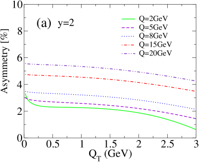
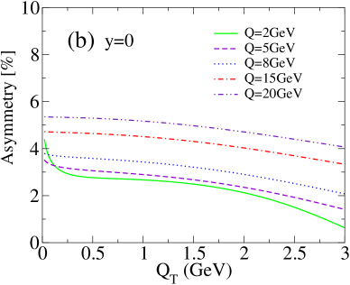
Figure 4: Same as Fig. 3, but for $\sqrt{S}=500$ GeV.

Fig. 4 is same as Fig. 3, but for another RHIC kinematics with $\sqrt{S}=500$ GeV. General behavior for the $Q_{T}$, $Q$ and $y$ dependence is similar as that in Fig. 3. Comparing the curves with the same values of $Q$, $y$ between Figs. 3 and 4, ${\mathscr{A}_{TT}(Q_{T})}$ are smaller for higher energy $\sqrt{S}=500$ GeV than those for $\sqrt{S}=200$ GeV. This reflects the smaller $x_{1,2}^{0}=e^{\pm y}Q/\sqrt{S}$ for larger $\sqrt{S}$, and the corresponding enhancement of the denominator in (20). Similarly as Fig. 3, the NLL+LO ${\mathscr{A}_{TT}(Q_{T})}$ in the flat region of Fig. 4 are larger by 20-30% than the corresponding NLO $A_{TT}$ shown in Table 1. It is generally true, regardless of the specific kinematics or the detailed behavior of nonperturbative inputs, that the NLL+LO ${\mathscr{A}_{TT}(Q_{T})}$ of (20) in the flat region is considerably larger than the corresponding NLO $A_{TT}$, because this phenomenon is mainly governed by the partonic mechanism associated with the soft gluon resummation at the NLL level, as demonstrated in Figs. 1, 2. On the other hand, apparently the absolute magnitude of both ${\mathscr{A}_{TT}(Q_{T})}$ and $A_{TT}$ is influenced by the detailed behavior of the input parton distributions, in particular, by their small-$x$ behavior at RHIC. For example, if we change the input parton distributions, explained above (22), from the NLO GRV98 and GRSV2000 distributions into the NLO GRV94 [23] and GRSV96 [24] distributions, the NLO values of $A_{TT}$ become smaller by 30-40% than the corresponding values in Table 1. We note that the latter distributions are the ones used in the calculation of [4], and the small-$x$ behavior of the transversity distributions, resulting from $\delta q(x,\mu^{2}_{0})=[q(x,\mu^{2}_{0})+\Delta q(x,\mu^{2}_{0})]/2$ at the input scale $\mu_{0}$, is rather different between those two choices of the distributions, reflecting that the helicity distributions at small $x$ are still poorly determined from experiments. 

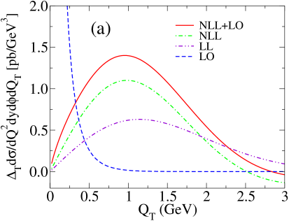
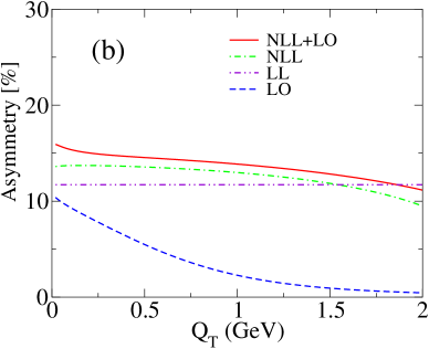
Figure 5: The tDY at J-PARC kinematics, $\sqrt{S}=10$ GeV, $Q=2$ GeV, $y=0$ and $\phi=0$. (a) The spin-dependent differential cross section $\Delta_{T}d\sigma/dQ^{2}dQ_{T}dyd\phi$ using $g_{NP}=0.5$ GeV². (b) The asymmetries ${\mathscr{A}_{TT}(Q_{T})}$ obtained by using each curve in (a).

Next we discuss tDY foreseen at J-PARC. Fig. 5(a) shows the $Q_{T}$ spectrum of the produced lepton pair for J-PARC kinematics, $\sqrt{S}=10$ GeV, $Q=2$ GeV and $y=0$. The curves show the spin-dependent differential cross sections, and have the same meaning as the corresponding curves in Fig. 1(a). The double transverse-spin asymmetries are obtained as the ratio of the results in Fig. 5(a) to the corresponding results for the unpolarized differential cross sections, as shown in Fig. 5(b). We see that the results at J-PARC obey the similar pattern as those at RHIC shown in Figs. 1, 2: the flat behavior is observed for the NLL+LO ${\mathscr{A}_{TT}(Q_{T})}$ at $Q_{T}\rightarrow 0$ as well as around the peak region of the NLL+LO cross section, and this is dominated by the NLL resummed components. Also the soft-gluon resummation contributions at the NLL level enhances the asymmetry at the small $Q_{T}$-region significantly, compared with the LL of (24) or the fixed-order LO result. As a result, we get ${\mathscr{A}_{TT}(Q_{T})}\simeq 15$% as the NLL+LO prediction around the flat region, which should be compared with the corresponding prediction $A_{TT}=12.8$% for (2) including the NLO corrections (see Table 2). The reason why we obtain much larger values of ${\mathscr{A}_{TT}(Q_{T})}$, and also of $A_{TT}$, than the RHIC case is the larger $x_{1,2}^{0}=0.2$ probed at J-PARC, where the transversities are larger and the unpolarized sea distributions are smaller. Another difference compared with the RHIC case is that the contribution of the “regular component” $\Delta_{T}\tilde{Y}$ of (17) in Fig. 5(a), and the associated increase of the solid curve as $Q_{T}\rightarrow 0$ in Fig. 5(b), due to the terms $\propto\ln(Q^{2}/Q_{T}^{2})$ in $\Delta_{T}\tilde{Y}$ and $\tilde{Y}$ of (20), are more pronounced, but the latter effect shows up only for $Q_{T}\lesssim 0.5$ GeV.

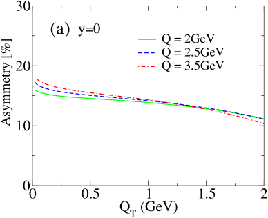
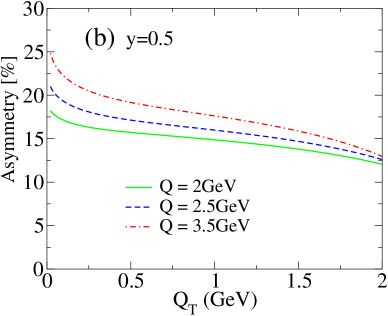
Figure 6: The NLL+LO ${\mathscr{A}_{TT}(Q_{T})}$ of (20) with (22) using $g_{NP}=0.5$ GeV² at J-PARC kinematics, $\sqrt{S}=10$ GeV, $\phi=0$ with $y=0$ and $y=0.5$ for (a) and (b), respectively.

		$Q=2$GeV	$Q=2.5$GeV	$Q=3.5$GeV
$\sqrt{S}=10$GeV	$y=0$	12.8%	12.9%	12.5%
	$y=0.5$	13.9%	14.8%	15.9%

Table 2: Same as Table 1 but for J-PARC kinematics.

In Fig. 6 we show the NLL+LO asymmetries ${\mathscr{A}_{TT}(Q_{T})}$ of (20) at J-PARC kinematics, $\sqrt{S}=10$ GeV and various values of $Q$, with $y=0$ and $y=0.5$ for (a) and (b), respectively; the solid curve in (a) is the same as the solid curve in Fig. 5(b). We observe the flat behavior of ${\mathscr{A}_{TT}(Q_{T})}$ in the small $Q_{T}$ region, where ${\mathscr{A}_{TT}(Q_{T})}\simeq 15$-20% and these values are significantly larger than the corresponding results for the $Q_{T}$-independent, NLO asymmetry $A_{TT}$ of (2), shown in Table 2. We note that the dependence of ${\mathscr{A}_{TT}(Q_{T})}$, as well as $A_{TT}$, on $Q$ is weak in contrast to the RHIC case; recall that the rather strong $Q$-dependence in Figs. 3, 4 was induced mainly by the growth of the unpolarized sea-distributions for the small $x_{1,2}^{0}$, probed at RHIC.

4 The saddle point formula

In Sec. 3, we have observed the universal flat behavior of NLL+LO ${\mathscr{A}_{TT}(Q_{T})}$ of (20) at small $Q_{T}$, including the region around the peak of each DY cross section in the numerator and denominator of (20) for both RHIC and J-PARC cases. We have also demonstrated in Figs. 2 and 5 that those flat behavior is driven by the dominant effects from soft gluon resummation embodied by the NLL resummed components $\Delta_{T}\tilde{X}^{\rm NLL}$ and $\tilde{X}^{\rm NLL}$ in (20). As a result, the values of ${\mathscr{A}_{TT}(Q_{T})}$ obtained in the “flat region” of the corresponding experimental data may be compared, to a good accuracy, with (23). Still, extraction of transversity distributions through such analysis should be a complicated task compared with the usual fixed-order analysis: in the flat region of ${\mathscr{A}_{TT}(Q_{T})}$, the $b$ integration in the resummed part (4) (see also (14), (15)) mixes up the parton distributions numerically with very large perturbative effects due to the Sudakov factor shown in Figs. 1 and 5, as well as with another nonperturbative effects associated with $g_{NP}$ of (22). Thus in each of the numerator and the denominator of (20), the information on the parton distributions is associated with a portion of the large numerical quantity whose major part would cancel in the ratio of (20), and this fact would obscure the straightforward extraction of the transversity using the above formulae like (14), (15), in particular with respect to its accuracy.

We are able to derive a simple analytic formula which allows more direct extraction of the transversity distributions from the experimental data in the flat region of ${\mathscr{A}_{TT}(Q_{T})}$ and also clarifies the accuracy of the resulting distributions. For this purpose, we first note that the extrapolation of ${\mathscr{A}_{TT}(Q_{T})}$ in the flat region to $Q_{T}=0$ corresponds to the case without the (experimentally uninteresting) weak enhancement at very small $Q_{T}$ due to the terms $\propto\log(Q^{2}/Q_{T}^{2})$ in the regular components $\Delta_{T}\tilde{Y}$ and $\tilde{Y}$ of (20), so that the resulting value is very close to the $Q_{T}\rightarrow 0$ limit of (23) in both RHIC and J-PARC cases (see Figs. 2-6). Namely, $\mathscr{A}_{TT}^{\rm NLL}(Q_{T}=0)$ may be considered to give a practical estimate of the data of ${\mathscr{A}_{TT}(Q_{T})}$ in the flat region with a good accuracy. Then, at $Q_{T}=0$, the region $|b|\sim 1/\Lambda_{\rm QCD}$ becomes important for the $b$ integration of the relevant resummation formula (15). Note that we can treat “safely” such long-distance region, corresponding to the boundary of perturbative and nonperturbative physics, owing to that the nonperturbative smearing (22) suppresses the too long-distance region $|b|\gg 1/\Lambda_{\rm QCD}$, and that the dependence on a specific choice of $g_{NP}$ cancels in the asymmetries $\mathscr{A}_{TT}^{\rm NLL}(Q_{T}=0)$ as demonstrated in Fig. 2(b) (see also (30) below).

For simplicity in the presentation, we fix as $\mu_{R}=Q$ in the following. In the relevant region $|b|\sim 1/\Lambda_{\rm QCD}$, we have $|\tilde{L}|\sim\ln(Q^{2}/\Lambda_{\rm QCD}^{2})\sim 1/\alpha_{s}(Q^{2})$, i.e., $|\lambda|\sim 1$ (see (16), (11)). Because all logarithms, $\tilde{L}$ and $\ln(Q^{2}/\Lambda^{2}_{\rm QCD})$, are counted equally large for $Q\gg\Lambda_{\rm QCD}$, the resulting contributions to (15) are organized in terms of a single small parameter, $\alpha_{s}(Q^{2})$, but with a different classification of the contributions in the order of $\alpha_{s}(Q^{2})$ from the usual perturbation theory that can be used in an other region, $0\leq|b|\lesssim 1/Q$: as discussed below (11), when $\lambda={\cal O}(1)$, the NLL contributions in the Sudakov exponent (8) produce the ${\cal O}(1)$ effects in the resummation formula (15), while the NNLL contributions could yield the corrections of ${\cal O}(\alpha_{s}(Q^{2}))$. Therefore, when the region $|b|\sim 1/\Lambda_{\rm QCD}$ is relevant as $Q_{T}\rightarrow 0$ and we neglect the NNLL contributions in (15), the other contributions that correspond to the same order of $\alpha_{s}(Q^{2})$ in (14) should be neglected for a consistent treatment, as $[1+\alpha_{s}(Q^{2})C_{F}(\pi^{2}-8)/2\pi]\rightarrow 1$, so that 

$$\Delta_{T}X^{\rm NLL}_{N_{1},N_{2}}(Q_{T}^{2}=0,Q^{2})=\delta H_{N_{1},N_{2}}(Q^{2})I_{N_{1},N_{2}}(Q_{T}^{2}=0,Q^{2})\ .$$ (25)

We note that the contributions to the NLL resummation formula for the unpolarized case can be classified similarly in the $Q_{T}\rightarrow 0$ limit; in particular, the present classification implies that the gluon distributions decouple for $Q_{T}\rightarrow 0$ by negelecting the ${\cal O}(\alpha_{s}(Q^{2}))$ contributions of the corresponding coefficient functions $C_{ij}$ (see (31) in Appendix).

It is also worth noting that this classification coincides with the “degree 0 approximation” discussed in [15]: in general, if one wants to evaluate the cross section for $Q_{T}\approx 0$ in an approximation where any corrections are suppressed by a factor of $[\ln(Q^{2}/\Lambda^{2}_{\rm QCD})]^{-(N+1)}$, one needs a “degree $N$” approximation; i.e., for the perturbatively calculable functions in the general form of resummation formula (4) with (5), one needs $A_{q}$ to order $\alpha_{s}^{N+2}$, $B_{q}$ to order $\alpha_{s}^{N+1}$, $C_{ij}$ to order $\alpha_{s}^{N}$, and the $\beta$ function to order $\alpha_{s}^{N+2}$. This indicates that the NLL accuracy for a resummation formula corresponds to the degree 0 approximation when the region $Q_{T}\approx 0$ is considered. In particular, this implies that the ${\cal O}(\alpha_{s})$ contribution in the coefficient function $C_{ij}$ should be neglected for $Q_{T}\approx 0$; on the other hand, that contribution is necessary to ensure the NLL accuracy for $Q_{T}\gtrsim\Lambda_{\rm QCD}$ in the classification based on resummed perturbation theory of towers of logarithms, $\alpha_{s}^{n}\ln^{2n-1}(Q^{2}/Q_{T}^{2})/Q_{T}^{2}$, $\alpha_{s}^{n}\ln^{2n-2}(Q^{2}/Q_{T}^{2})/Q_{T}^{2}$, and $\alpha_{s}^{n}\ln^{2n-3}(Q^{2}/Q_{T}^{2})/Q_{T}^{2}$ [15, 14, 6].

Now we evaluate the $b$ integral of (15) at $Q_{T}=0$ according to the above classification. We have to use the exponentiated form in the integrand of (15) without Taylor expansion, because the region $|\lambda|\sim 1$ is relevant (see (8)-(13)) [26]. This type of integrals can be evaluated with the saddle point method: we extend the saddle point evaluation applied to the LL resummation formula with $g_{NP}=0$ [25, 15] into the case of our NLL resummation formula (15) with nonzero $g_{NP}$. The corresponding extension is possible based on the present formalism that accomplishes resummation at the partonic level. We note that previous saddle-point calculations consider the case with $g_{NP}=0$ to avoid model dependence for the prediction of the cross sections, but the resultant saddle-point formula is applicable only to the production of extremely high-mass DY pair and is practically useless (see e.g. [25, 15, 27]). We find that, with nonzero $g_{NP}$, we can obtain a new saddle-point formula applicable to the RHIC and J-PARC cases; also, although the behavior of the cross sections are influenced by specific value of $g_{NP}$, the asymmetries are not, as already noted above.

When $Q$ is large enough, $\alpha_{s}(Q^{2})\ll 1$, so that the $b$ integral in (15) with (22) and $Q_{T}=0$ is dominated by a saddle point determined by mainly the LL term in the exponent (8) of the Sudakov form factor [25, 15]. In this case, the contributions to the $b$ integration from too short ($|b|\ll 1/Q$) and long distance ($|b|\gg 1/\Lambda_{\rm QCD}$) along the integration contour ${\cal C}$ explained below (16) are exponentially suppressed: this allows us to give up the replacement (16); also we may neglect the integration along the two branches, $b=b_{c}+e^{\pm i\theta}t$ with $t\in\{0,\infty\}$, in ${\cal C}$, when $b_{c}$ is sufficiently large but is less than the position of the singularity in the Sudakov exponent, $b_{L}$. In fact, we can check numerically that the relevant integrand has a nice saddle point well below $b_{L}$ (above $0$) for the kinematics of our interest. Then, changing the integration variable to $\lambda$, given by (11), we get (see (9), (10), (13))

$$I_{N_{1},N_{2}}(Q_{T}^{2}=0,Q^{2})=\frac{b_{0}^{2}}{4Q^{2}\beta_{0}\alpha_{s}(Q^{2})}\int_{-\infty}^{\lambda_{c}}d\lambda e^{-\zeta(\lambda)+h^{(1)}(\lambda)+R_{N_{1}}(\lambda)+R_{N_{2}}(\lambda)}\ ,$$ (26)

where $\lambda_{c}=\beta_{0}\alpha_{s}(Q^{2})\ln(Q^{2}b_{c}^{2}/b_{0}^{2})$ ($<1$), and

$$\zeta(\lambda)=-\frac{\lambda}{\beta_{0}\alpha_{s}(Q^{2})}-\frac{h^{(0)}(\lambda)}{\alpha_{s}(Q^{2})}+\frac{g_{NP}b_{0}^{2}}{Q^{2}}e^{\frac{\lambda}{\beta_{0}\alpha_{s}(Q^{2})}}\ .$$ (27)

An important point is that the ratio, $[h^{(1)}(\lambda)+R_{N_{1}}(\lambda)+R_{N_{2}}(\lambda)]/\zeta(\lambda)$, actually behaves as a quantity of the order of $\alpha_{s}(Q^{2})$ in the relevant region $0<\lambda<\lambda_{c}$ of the integration in (26), even for nonzero $g_{NP}\simeq 0.5$ GeV². The precise position of the saddle point in the integral of (26) is determined by the condition, $-{\zeta}^{\prime}(\lambda)+{h^{(1)}}^{\prime}(\lambda)+{R_{N_{1}}}^{\prime}(\lambda)+{R_{N_{2}}}^{\prime}(\lambda)=0$, and we express its solution as $\lambda=\lambda_{SP}+\Delta\lambda_{SP}$ where $\lambda_{SP}$ is the solution of $\zeta^{\prime}(\lambda)=0$, i.e.,

$$1-\frac{A_{q}^{(1)}}{2\pi\beta_{0}}\frac{\lambda_{SP}}{1-\lambda_{SP}}=\frac{g_{NP}b_{0}^{2}}{Q^{2}}e^{\frac{\lambda_{SP}}{\beta_{0}\alpha_{s}(Q^{2})}}$$ (28)

is satisfied, and $\Delta\lambda_{SP}=[{h^{(1)}}^{\prime}(\lambda_{SP})+{R_{N_{1}}}^{\prime}(\lambda_{SP})+{R_{N_{2}}}^{\prime}(\lambda_{SP})]/{\zeta}^{\prime\prime}(\lambda_{SP})$ denotes the shift of the saddle point at the NLL accuracy. Evaluating (26) around $\lambda=\lambda_{SP}+\Delta\lambda_{SP}$, we get

$$I_{N_{1},N_{2}}(0,Q^{2})=\left(\frac{b_{0}^{2}}{4Q^{2}\beta_{0}\alpha_{s}(Q^{2})}\sqrt{\frac{2\pi}{\zeta^{\prime\prime}(\lambda_{SP})}}e^{-\zeta(\lambda_{SP})+h^{(1)}(\lambda_{SP})}\right)e^{R_{N_{1}}(\lambda_{SP})+R_{N_{2}}(\lambda_{SP})},$$ (29)

to the NLL accuracy. Here the contributions from the third or higher order terms in the Taylor expansion of the exponent in (26) about the saddle point $\lambda=\lambda_{SP}+\Delta\lambda_{SP}$, as well as the other terms generated by the shift $\Delta\lambda_{SP}$, are found to give the effects behaving as ${\cal O}(\alpha_{s}(Q^{2}))$, i.e, are of the same order as the NNLL corrections, and thus are neglected, similarly as in (14), (25), according to the classification of the contributions at $Q_{T}=0$. Substituting (29) into (25) and performing the double inverse Mellin transformation to the ($x_{1}^{0}$, $x_{2}^{0}$) space, the result is expressed as the factor in the parentheses of (29), multiplied by (1) with the scale, $\mu_{F}\rightarrow b_{0}/b_{SP}$ where $b_{SP}=(b_{0}/Q)e^{\lambda_{SP}/(2\beta_{0}\alpha_{s}(Q^{2}))}$, because $e^{R_{N_{1}}(\lambda_{SP})}$, $e^{R_{N_{2}}(\lambda_{SP})}$ in (29) can be identified with the NLO evolution operators from the scale $Q$ to $b_{0}/b_{SP}$, to the present accuracy (see (13)). The saddle-point evaluation of the corresponding resummation formula for the unpolarized case can be performed similarly, and the result is given by the above result for the polarized case, with the replacement $\delta H(x_{1}^{0},x_{2}^{0};\ b_{0}^{2}/b_{SP}^{2})\rightarrow H(x_{1}^{0},x_{2}^{0};\ b_{0}^{2}/b_{SP}^{2})$. The common factor for both the polarized and unpolarized results, given by the contribution in the parentheses of (29), involves “very large perturbative effects” due to the Sudakov factor, and shows the well-known asymptotic behavior [25], $\sim(\Lambda_{\rm QCD}^{2}/Q^{2})^{a\ln(1+1/a)}$ with $a\equiv A_{q}^{(1)}/(2\pi\beta_{0})$, for $Q\gg\Lambda_{\rm QCD}$; but this factor cancels out for the asymmetry. As a result, we obtain the $Q_{T}\rightarrow 0$ limit of (23) as

$$\mathscr{A}_{TT}^{\rm NLL}(Q_{T}=0)=\frac{1}{2}\cos(2\phi)\frac{\delta H\left(x_{1}^{0},x_{2}^{0};\ b_{0}^{2}/b_{SP}^{2}\right)}{H\left(x_{1}^{0},x_{2}^{0};\ b_{0}^{2}/b_{SP}^{2}\right)}\ ,$$ (30)

which is exact, up to the NNLL corrections corresponding to the ${\cal O}(\alpha_{s}(Q^{2}))$ effects. This remarkably compact formula is reminiscent of $\mathscr{A}_{TT}^{\rm LL}(Q_{T})$ of (24) that retains only the LL level resummation, or the $Q_{T}$ independent asymmetry of (2), but is different in the scale of the parton distributions from those leading-order results. Namely, our result (30) demonstrates: in the $Q_{T}=0$ limit, the all-order soft-gluon-resummation effects on the asymmetry mostly cancel between the numerator and the denominator of (30), but certain contributions at the NLL level survive the cancellation and are entirely absorbed into the unconventional scale $b_{0}/b_{SP}$ for the relevant distribution functions.

The new scale $b_{0}/b_{SP}$ is determined by solving (28) numerically, substituting $A_{q}^{(1)}=2C_{F}$ from (6) and input values for $Q$ and $g_{NP}$, but it is useful to consider its general behavior: the LHS of (28) equals 1 at $\lambda_{SP}=0$, decreases as a concave function for increasing $\lambda_{SP}$, and vanishes at $\lambda_{SP}=1/[1+A_{q}^{(1)}/(2\pi\beta_{0})]\cong 0.6$; while the RHS is in general much smaller than 1 at $\lambda_{SP}=0$, increases as a convex function for increasing $\lambda_{SP}$, and is larger than 1 at $\lambda_{SP}\simeq 1$. Thus the solution of (28) corresponds to the case with ${\rm LHS}={\rm RHS}\simeq 1/2$, more or less independently of the specific value of $Q$ and $g_{NP}$, so that we get $b_{0}/b_{SP}\simeq b_{0}\sqrt{2g_{NP}}$. This result depends only mildly on the nonperturbative parameter $g_{NP}$, and suggests that one may always use $b_{0}/b_{SP}\simeq 1$ GeV, for the cases of our interest where $Q$ is of several GeV and $g_{NP}\simeq 0.5$ GeV² as in Figs. 1-6. The actual numerical solution of (28) justifies this simple consideration at the level of 20% accuracy. This fact will be particularly helpful in the first attempt to compare (30) with the experimental data so as to extract the transversity distributions.

Our saddle-point formula (30) embodies the characteristic features of the NLL soft gluon resummation effects on the asymmetries ${\mathscr{A}_{TT}(Q_{T})}$, emphasized in Sec. 3. In particular, our derivation of (30) demonstrates clearly the mechanism, which makes the parton distributions at the low scale $\sim Q_{T}$ play dominant roles, and leads to the “enhancement” of the dot-dashed curve in Figs. 2 and 5. As noted in the beginning of this section, (30) may be directly compared with the experimental value of the asymmetries ${\mathscr{A}_{TT}(Q_{T})}$, observed around the peak of the $Q_{T}$ spectrum of the corresponding DY cross sections. But there is one caution for such application. As seen from the above derivation, the parton distributions appearing in (30) are the NLO distributions up to the corrections at the NNLL level; e.g., the transversity distributions appearing in the numerator of (30) is obtained by evolving the customary NLO transversity $\delta q(x,Q^{2})$ at the scale $Q$, to the scale $b_{0}/b_{SP}$ using (13) that is the NLO evolution operators up to the NNLL corrections. Therefore, the formula (30) can be used in the region where NNLL corrections are small; we know that the NNLL corrections at $Q_{T}\approx 0$ correspond to ${\cal O}(\alpha_{s}(Q^{2}))$ effects, and should be negligible in general. However, such straightforward estimate might fail at the edge region of the phase space, e.g., at the small $x$ region: because the relevant evolution operators (13) actually coincide with the leading contributions in the large-logarithmic expansion of the usual LO DGLAP evolution, (30) would not accurate when the NLO corrections in the usual DGLAP evolution are large compared with the contributions of (13). Such situation would typically occur in the region with small $x_{1,2}^{0}$, corresponding to the case with large $\sqrt{S}$. In Table 3, we compare $\mathscr{A}_{TT}^{\rm NLL}(Q_{T}=0)$ using the numerical $b$-integration (“NB”), obtained as the $Q_{T}\rightarrow 0$ limit of the dot-dashed curve in Figs 3(a) and 6(a), with those using the saddle-point formula (30). For the latter we use $b_{0}/b_{SP}$ obtained as the solution of (28) with $g_{NP}=0.5$ GeV², and consider the two cases for the parton distributions participating in (30): “SP-I” uses the parton distributions which are obtained by evolving the customary NLO distributions at the scale $Q$, to $b_{0}/b_{SP}$ using the NLO evolution operators up to the NNLL corrections like (13); “SP-II” uses the customary NLO distributions at the scale $b_{0}/b_{SP}$. Here the “customary NLO distributions” are constructed as described above (22). First of all, the results for SP-I demonstrate the remarkable accuracy of our simple analytic formula (30) for both RHIC and J-PARC, reproducing the results of NB to the 10% accuracy.  On the other hand, the results for SP-II indicate that the NNLL corrections are moderate for large $\sqrt{S}$ at RHIC, while those are expected to be small for small $\sqrt{S}$ at J-PARC.

We propose that our simple formula (30) is applicable to the analysis of low-energy experiment at J-PARC in order to extract the NLO transversity distributions directly from the data. On the other hand, (30) will not be so accurate for analyzing the data at RHIC, but will be still useful for obtaining the first estimate of the transversities. We emphasize that such (moderate) uncertainty in applying our formula (30) to the RHIC case is not caused by the saddle-point evaluation, nor by considering the $Q_{T}\rightarrow 0$ limit, but rather is inherent in the general $Q_{T}$ resummation framework which, at the NLL level, implies the use of the evolution operators (13) with the LO DGLAP kernel; more accurate treatment of the small-$x$ region of the parton distributions relevant to the RHIC case would require the resummation formula to the NNLL accuracy, where the NLO DGLAP kernel participates in the evolution operators (13) from $Q$ to $b_{0}/b$ (see e.g. [14]).

	$\sqrt{S}=200$ GeV,   $y=2$					$\sqrt{S}=10$ GeV,   $y=0$
$Q$	2GeV	5GeV	8GeV	15GeV	20GeV	2GeV	2.5GeV	3.5GeV
SP-I	4.3%	5.4%	6.6%	8.7%	9.8%	14.1%	14.5%	14.8%
SP-II	7.3%	8.7%	9.8%	11.8%	12.7%	14.7%	14.8%	14.2%
NB	3.8%	4.9%	6.1%	8.2%	9.4%	13.4%	14.0%	14.9%

Table 3: The $Q_{T}\rightarrow 0$ limit of $\mathscr{A}_{TT}^{\rm NLL}(Q_{T})$ of (23) for RHIC and J-PARC kinematics. SP-I and SP-II are the results of the saddle-point formula (30) for $g_{NP}=0.5$ GeV², using the evolution operators from $Q$ to $b_{0}/b_{SP}$, to the NLL accuracy and to the customary NLO accuracy, respectively. NB is obtained from the dot-dashed curve in Figs 3(a) and 6(a).

5 Conclusions

In this paper we have presented a study of double transverse-spin asymmetries for dilepton production at small $Q_{T}$ in $pp$ collisions. The logarithmically enhanced contributions, which arise in the small $Q_{T}$ region due to multiple soft gluon emission in QCD, are resummed to all orders in $\alpha_{s}$ up to the NLL accuracy. Based on this framework, we calculate numerically the spin-dependent and spin-averaged cross sections in tDY, and the corresponding asymmetries ${\mathscr{A}_{TT}(Q_{T})}$, as a function of $Q_{T}$ at RHIC kinematics as well as at J-PARC kinematics. The soft gluon resummation contributions make the cross sections finite and well-behaved over all regions of $Q_{T}$, so that the singular $Q_{T}$ spectra in the fixed-order perturbation theory are redistributed, forming a well-developed peak in the small $Q_{T}$ region. As a result, both the polarized and unpolarized cross sections become more “observable” around the pronounced “peak region” at small $Q_{T}$, involving the bulk of events. Reflecting the universal nature of the soft gluon effects, those large resummation-contributions mostly cancel in the cross section asymmetries ${\mathscr{A}_{TT}(Q_{T})}$, leading to the almost constant behavior of ${\mathscr{A}_{TT}(Q_{T})}$ in the small $Q_{T}$ region, but, remarkably, the effects surviving the cancellation raise the corresponding constant value of ${\mathscr{A}_{TT}(Q_{T})}$ considerably compared with the asymmetries in the fixed-order perturbation theory. We have obtained a QCD prediction as ${\mathscr{A}_{TT}(Q_{T})}\simeq 5$-10% and 15-20% in the “flat region” for typical kinematics at RHIC and J-PARC, respectively, where the different values of ${\mathscr{A}_{TT}(Q_{T})}$ are associated with the different values of parton’s momentum fraction probed by these two experiments.

We have also derived a new saddle-point formula for $\mathscr{A}_{TT}(Q_{T}\approx 0)$, clarifying the classification of the contributions involved in the resummation formula for $Q_{T}\rightarrow 0$. The formula is exact to the NLL accuracy, and embodies the above remarkable features of soft gluon resummation effects at small $Q_{T}$ in a compact analytic form. Our saddle-point formula may be compared with the data of ${\mathscr{A}_{TT}(Q_{T})}$ in the peak region of the DY $Q_{T}$-spectrum, and thus provides us with a new direct approach to extract the transversity distributions from experimental data.

We mention that there is another kind of logarithmically enhanced soft-gluon contributions, subject to the so-called “threshold resummation”, besides those treated by the $Q_{T}$ resummation. It is known that the threshold resummation effects on the cross sections can be important when the probed momentum fractions of partons are rather large like at J-PARC. The corresponding effects for tDY are studied [28] in $p\bar{p}$ collisions at GSI kinematics, and the results indicate that the threshold resummation effects will not be so significant for the kinematical regions corresponding to experiments at J-PARC, and, furthermore, will cancel mostly in the asymmetries.

We have revealed that the “amplification” of the double transverse-spin asymmetries ${\mathscr{A}_{TT}(Q_{T})}$ at small $Q_{T}$ is driven by the partonic mechanism participating at the NLL level, as the interplay between the large logarithmic gluon effects resummded into the universal Sudakov factor and the DGLAP evolutions specific for each channel. Thus similar phenomenon is anticipated also in $p\bar{p}$ collisions at the future experiments at GSI [29], where the large values are predicted for the $Q_{T}$ independent asymmetry $A_{TT}$ [28, 30]. The application of our $Q_{T}$ resummation formalism to $p\bar{p}$ collision will be presented elsewhere [31].

Appendix: Resummed cross section for unpolarized DY

In this appendix, we summarize the corresponding results for the unpolarized Drell-Yan process which are necessary to calculate the asymmetry ${\mathscr{A}_{TT}(Q_{T})}$. Although all of them have already appeared in the literatures [18, 15], we will list them for the convenience of the reader.

The NLL resummed component, corresponding to (4) for the polarized case, reads,

$$X^{\rm NLL}(Q_{T}^{2},Q^{2},y)=\int_{0}^{\infty}db\,\frac{b}{2}\,J_{0}(bq_{T})\,e^{\,S(b,Q)}\ \biggl{[}H(x_{1}^{0}\,,\,x_{2}^{0}\,;\,b^{2}_{0}/b^{2})$$ (31)

$$+ \frac{\alpha_{s}(b^{2}_{0}/b^{2})}{2\pi}\left\{\int_{x_{1}^{0}}^{1}\frac{dz}{z}\,C_{qq}^{(1)}(z)\,H(x_{1}^{0}/z\,,\,x_{2}^{0}\,;\,b^{2}_{0}/b^{2})+\int_{x_{2}^{0}}^{1}\frac{dz}{z}\,C_{qq}^{(1)}(z)\,H(x_{1}^{0}\,,\,x_{2}^{0}/z\,;\,b^{2}_{0}/b^{2})\right.$$

$$+ \left.\int_{x_{1}^{0}}^{1}\frac{dz}{z}\,C_{qg}^{(1)}(z)\,K_{2}(x_{1}^{0}/z\,,\,x_{2}^{0}\,;\,b^{2}_{0}/b^{2})+\int_{x_{2}^{0}}^{1}\frac{dz}{z}\,C_{qg}^{(1)}(z)\,K_{1}(x_{1}^{0}\,,\,x_{2}^{0}/z\,;\,b^{2}_{0}/b^{2})\right\}\,\biggr{]}\ ,$$

where $S(b,Q)$ is the exponent of the Sudakov factor, given by (5)-(11), and

$$C_{qq}^{(1)}(z) = C_{\bar{q}\bar{q}}^{(1)}(z)=C_{F}\,(1-z)+C_{F}\left(\frac{\pi^{2}}{2}-4\right)\,\delta(1-z)\ ,$$

$$C_{qg}^{(1)}(z) = C_{\bar{q}g}^{(1)}(z)=2\,T_{R}\,z(1-z)\ ,$$

with $T_{R}=1/2$. The parton distributions are defined as,

$$H(x_{1}\,,\,x_{2};\,\mu_{F}^{2}) = \sum_{q}\,e_{q}^{2}\,\left[q(x_{1},\mu_{F}^{2})\,\bar{q}(x_{2},\mu_{F}^{2})+\bar{q}(x_{1},\mu_{F}^{2})\,q(x_{2},\mu_{F}^{2})\right]\ ,$$

$$K_{1}(x_{1}\,,\,x_{2};\,\mu_{F}^{2}) = \sum_{q}\,e_{q}^{2}\,\left[q(x_{1},\mu_{F}^{2})+\bar{q}(x_{1},\mu_{F}^{2})\right]\,g(x_{2},\mu_{F}^{2})\ ,$$

$$K_{2}(x_{1}\,,\,x_{2};\,\mu_{F}^{2}) = \sum_{q}\,e_{q}^{2}\,g(x_{1},\mu_{F}^{2})\,\left[q(x_{2},\mu_{F}^{2})+\bar{q}(x_{2},\mu_{F}^{2})\right]\ .$$

The finite component, corresponding to $\Delta_{T}Y$ of (3) for the polarized case, is given by,

$$Y(Q_{T}^{2}\,,\,Q^{2}\,,\,y)=\frac{\alpha_{s}(\mu_{R}^{2})}{2\pi}\,\left[C_{F}\,Y_{q}(Q_{T}^{2}\,,\,Q^{2}\,,\,y)+T_{R}\,Y_{g}(Q_{T}^{2}\,,\,Q^{2}\,,\,y)\right]\ ,$$

where the first term comes from the $q\bar{q}$ annihilation subprocess as

$$Y_{q}(Q_{T}^{2}\,,\,Q^{2}\,,\,y) = -\,\frac{2}{S}\left[\int^{1}_{\sqrt{\tau_{+}}\,e^{y}}\,\frac{dx_{1}}{x_{1}-x_{1}^{+}}\ \frac{H(x_{1}\,,\,x_{2}^{*};\,\mu_{F}^{2})}{x_{1}x_{2}^{*}}+\int^{1}_{\sqrt{\tau_{+}}\,e^{-y}}\,\frac{dx_{2}}{x_{2}-x_{2}^{+}}\ \frac{H(x_{1}^{*}\,,\,x_{2};\,\mu_{F}^{2})}{x_{1}^{*}x_{2}}\right]$$

$$+ \frac{1}{Q_{T}^{2}}\,\left[\int dx_{1}\,H_{1}+\int dx_{2}\,H_{2}+2\,H(x_{1}^{0}\,,\,x_{2}^{0};\,\mu_{F}^{2})\,\ln\frac{(1-x_{1}^{+})(1-x_{2}^{+})}{(1-x_{1}^{0})(1-x_{2}^{0})}\right]\ ,$$

with the variables according to [18, 6]:

$$x_{1}^{+} = \left(\frac{Q^{2}+Q^{2}_{T}}{S}\right)^{1/2}e^{y}\ ,\quad x_{2}^{+}=\left(\frac{Q^{2}+Q^{2}_{T}}{S}\right)^{1/2}e^{-y}\ ,$$

$$x_{1}^{*} = \frac{x_{2}x_{1}^{+}-x_{1}^{0}x_{2}^{0}}{x_{2}-x_{2}^{+}}\ ,\quad x_{2}^{*}=\frac{x_{1}x_{2}^{+}-x_{1}^{0}x_{2}^{0}}{x_{1}-x_{1}^{+}}\ ,\quad\sqrt{\tau_{+}}=\sqrt{\frac{Q_{T}^{2}}{S}}+\sqrt{\tau+\frac{Q_{T}^{2}}{S}}\ .$$

We used the shorthand notation for the integral that vanishes for $Q_{T}=0$,

$$\int dx_{1}\,H_{1} \equiv \int^{1}_{\sqrt{\tau_{+}}\,e^{y}}\ \,\frac{dx_{1}}{x_{1}-x_{1}^{+}}\left[H(x_{1}\,,\,x_{2}^{*};\,\mu_{F}^{2})\left\{1+\left(\frac{\tau}{x_{1}x_{2}^{*}}\right)^{2}\right\}-2\,H(x_{1}^{0}\,,\,x_{2}^{0};\,\mu_{F}^{2})\right]$$

$$\qquad\qquad-\int^{1}_{x_{1}^{0}}\ \,\frac{dx_{1}}{x_{1}-x_{1}^{0}}\left[H(x_{1}\,,\,x_{2}^{0};\,\mu_{F}^{2})\left\{1+\left(\frac{x_{1}^{0}}{x_{1}}\right)^{2}\right\}-2\,H(x_{1}^{0}\,,\,x_{2}^{0};\,\mu_{F}^{2})\right]\ ,$$

and $\int dx_{2}\,H_{2}=\left.\int dx_{1}\,H_{1}\right|_{y\rightarrow-y}$. For the contribution from the gluon Compton process, we have

$$Y_{g}(Q_{T}^{2}\,,\,Q^{2}\,,\,y) = \frac{1}{S}\left[\int^{1}_{\sqrt{\tau_{+}}\,e^{y}}\,\frac{dx_{1}}{x_{1}-x_{1}^{+}}\ K_{1}(x_{1}\,,\,x_{2}^{*};\,\mu_{F}^{2})\frac{x_{1}x_{2}^{+}-\tau}{(x_{1}x_{2}^{*})^{2}}\right.$$

$$\qquad\qquad\qquad\qquad+\,\left.\int^{1}_{\sqrt{\tau_{+}}\,e^{-y}}\,\frac{dx_{2}}{x_{2}-x_{2}^{+}}\ K_{1}(x_{1}^{*}\,,\,x_{2};\,\mu_{F}^{2})\frac{x_{1}^{*}x_{2}^{+}-\tau}{(x_{1}^{*}x_{2})^{2}}\right]$$

$$+ \frac{1}{Q_{T}^{2}}\,\left[\int^{1}_{\sqrt{\tau_{+}}\,e^{-y}}\,\frac{dx_{2}}{x_{2}-x_{2}^{+}}\ K_{1}(x_{1}^{*}\,,\,x_{2};\,\mu_{F}^{2})\left\{\frac{x_{2}x_{1}^{+}-\tau}{x_{1}^{*}x_{2}}-\frac{2\,\tau\,(x_{2}x_{1}^{+}-\tau)^{2}}{(x_{1}^{*}x_{2})^{3}}\right\}\right.$$

$$\qquad\qquad\qquad\qquad-\,\int^{1}_{x_{2}^{0}}\,\frac{dx_{2}}{x_{2}}\ K_{1}(x_{1}^{0}\,,\,x_{2};\,\mu_{F}^{2})\left\{1-\frac{2\,x_{2}^{0}\,(x_{2}-x_{2}^{0})}{x_{2}^{2}}\right\}$$

$$\quad+\left.\int^{1}_{\sqrt{\tau_{+}}\,e^{y}}\,\frac{dx_{1}}{x_{1}-x_{1}^{+}}\ K_{1}(x_{1}\,,\,x_{2}^{*};\,\mu_{F}^{2})\left\{\frac{x_{2}^{*}x_{1}^{+}-\tau}{x_{1}x_{2}^{*}}-\frac{2\,\tau\,(x_{2}^{*}x_{1}^{+}-\tau)^{2}}{(x_{1}x_{2}^{*})^{3}}\right\}\right]$$

$$+ (1\leftrightarrow 2)\ ,$$

where $1\leftrightarrow 2$ means the exchange of the suffix of variables as well as $y\leftrightarrow-\,y$. As for the parton distributions, this exchange should be read,

$$K_{1}(x_{1}\,,\,x_{2}^{*})\leftrightarrow K_{2}(x_{1}^{*}\,,\,x_{2})\ ,\quad K_{1}(x_{1}^{*}\,,\,x_{2})\leftrightarrow K_{2}(x_{1}\,,\,x_{2}^{*})\ ,\quad K_{1}(x_{1}^{0}\,,\,x_{2})\leftrightarrow K_{2}(x_{1}\,,\,x_{2}^{0})\ .$$

The fixed-order cross section in the $\overline{\rm MS}$ scheme is given as

$$\frac{d\sigma^{\rm FO}}{dQ^{2}dQ_{T}^{2}dyd\phi}=\frac{2\alpha^{2}}{3\,N_{c}\,S\,Q^{2}}\left[X\,(Q_{T}^{2}\,,\,Q^{2}\,,\,y)+Y\,(Q_{T}^{2}\,,\,Q^{2}\,,\,y)\right],$$ (32)

to the ${\cal O}(\alpha_{s})$ accuracy, where $X\,(Q_{T}^{2}\,,\,Q^{2}\,,\,y)\equiv\left.X^{\rm NLL}\,(Q_{T}^{2}\,,\,Q^{2}\,,\,y)\right|_{\rm FO}$ denotes the “singular” part resulting from the expansion of the resummed component up to the fixed-order $\alpha_{s}(\mu_{R}^{2})$. The formula (32) should be compared with (3). Taking the similar steps as those in (12)-(17), we obtain the differential cross section for unpolarized DY with the soft gluon resummation as

$$\frac{d\sigma}{dQ^{2}dQ_{T}^{2}dyd\phi}=\frac{2\alpha^{2}}{3\,N_{c}\,S\,Q^{2}}\biggl{[}\tilde{X}^{\rm NLL}(Q_{T}^{2},Q^{2},y)+\tilde{Y}(Q_{T}^{2},Q^{2},y)\biggr{]},$$ (33)

which is used to calculate (20).

References

- [1] See e.g., V. Barone, A. Drago and P. G. Ratcliffe, Phys. Rep. 359, (2002) 1; J. Kodaira and K. Tanaka, Prog. Theor. Phys. 101 (1999) 191.
- [2] M. Anselmino, et al., Phys. Rev. D75 (2007) 054032.
- [3] J. P. Ralston and D. E. Soper, Nucl. Phys. B152 (1979) 109; R. L. Jaffe and X. D. Ji, Nucl. Phys. B375 (1992) 527.
- [4] O. Martin, A. Schäfer, M. Stratmann and W. Vogelsang, Phys. Rev. D57 (1998) 3084; ibid. D60 (1999) 117502.
- [5] A. Mukherjee, M. Stratmann and W. Vogelsang, Phys. Rev. D67 (2003) 114006; A. Mukherjee, M. Stratmann and W. Vogelsang, Phys. Rev. D72 (2005) 034011.
- [6] H. Kawamura, J. Kodaira, H. Shimizu and K. Tanaka, Prog. Theor. Phys. 115 (2006) 667.
- [7] D. Dutta et al., Letter of Intent (L15) for Nuclear and Particle Physics Experiments at J-PARC, http://www-ps.kek.jp/jhf-np/LOIlist/LOIlist.html.
- [8] Y. Koike, J. Nagashima and W. Vogelsang, Nucl. Phys. B744 (2006) 59.
- [9] M. Contalbrigo, A. Drago and P. Lenisa, hep-ph/0607143, in Proceedings of XIV International Workshop on Deep Inelastic Scattering (DIS2006), Tsukuba, Japan, eds. M. Kuze et al. (World Scientific, 2007), p.727.
- [10] C. T. H. Davies and W. J. Stirling, Nucl. Phys. B244 (1984) 337.
- [11] J. Kodaira and L. Trentadue, Phys. Lett. B112 (1982) 66 ; Report SLAC-Pub-2934 (1982); Phys. Lett. B123 (1983) 335.
- [12] D. de Florian and M. Grazzini, Phys. Rev. Lett. 85 (2000) 4678.
- [13] E. Laenen, G. Sterman and W. Vogelsang, Phys. Rev. D63 (2001) 114018; S. Kulesza, G. Sterman and W. Vogelsang, Phys. Rev. D66 (2002) 014011.
- [14] S. Catani, D. de Florian and M. Grazzini, Nucl. Phys. B596 (2001) 299; G. Bozzi, S. Catani, D. de Florian and M. Grazzini, Phys. Lett. B564 (2003) 65; Nucl. Phys. B737 (2006) 73.
- [15] J. C. Collins, D. Soper and G. Sterman, Nucl. Phys. B250 (1985) 199.
- [16] X. Artru and M. Mekhfi, Z. Phys. C45 (1990) 669.
- [17] A. Hayashigaki, Y. Kanazawa and Y. Koike, Phys. Rev. D56 (1997) 7350; S. Kumano and M. Miyama, Phys. Rev. D56 (1997) 2504; W. Vogelsang, Phys. Rev. D57 (1998) 1886.
- [18] G. Altarelli, R. K. Ellis, M. Greco and G. Martinelli, Nucl. Phys. B246 (1984) 12.
- [19] J. Soffer, Phys. Rev. Lett. 74 (1995) 1292.
- [20] M. Glück, E. Reya and A. Vogt, Eur. Phys. J. C5 (1998) 461.
- [21] M. Glück, E. Reya, M. Stratmann, and W. Vogelsang, Phys. Rev. D63 (2001) 094005.
- [22] A. Kulesza and W. J. Stirling, JHEP 0312 (2003) 056.
- [23] M. Gluck, E. Reya and A. Vogt, Z. Phys. C67 (1995) 433.
- [24] M. Gluck, E. Reya, M. Stratmann and W. Vogelsang, Phys. Rev. D53 (1996) 4775.
- [25] G. Parisi and R. Petronzio, Nucl. Phys. B154 (1979) 427; J. C. Collins and D. E. Soper, Nucl. Phys. B197 (1982) 446.
- [26] A. Kulesza and W. J. Stirling, Nucl. Phys. B555 (1999) 279.
- [27] J. Qiu and X. Zhang, Phys. Rev. Lett. 86 (2001) 2724.
- [28] H. Shimizu, G. Sterman, W. Vogelsang and H. Yokoya, Phys. Rev. D71 (2005) 114007.
- [29] V. Barone, et al.[PAX Collabolation], hep-ex/0505054; M. Maggiora et al. [ASSIA Collabolation], hep-ex/0504011.
- [30] V. Barone, A. Caferella, C .Coriano, M. Guzzi and P. G. Ratcliffe, Phys. Lett B639 (2006) 483.
- [31] H. Kawamura, J. Kodaira and K. Tanaka, in preparation.