New Physics with IceCube

Abstract

IceCube, a cubic kilometer neutrino telescope will be capable of probing neutrino-nucleon interactions in the ultrahigh energy regime, far beyond the energies reached by colliders. In this article we introduce a new observable that combines several advantages: it only makes use of the upward-going neutrino flux, so that the Earth filters the atmospheric muons, and it is only weakly dependent on the initial astrophysical flux uncertainties.

I Introduction

High precision or high energy are necessary to study the matter at short distances. The most powerful accelerators are the cosmic ones in the outer space. We know that the Earth is hit by cosmic rays of very high energy, which means that there have to be astrophysical mechanisms capable of accelerating protons to those high energies. It is then also possible that the same mechanisms could produce neutrinos of high energy or that the protons and radiation produced interact with matter to originate extremely high energy neutrinos. Some candidate neutrino sources are Active Galactic Nuclei (AGN) manh , which are the central regions of certain galaxies where the radiation emitted is comparable to the total radiation from the entire galaxy, and Gamma Ray Bursts (GRB) waxman , that are the most powerful explosions since the Big Bang resulting usually from the core collapse of massive stars.

The integrated effect over all astrophysical sources in the sky where such producing mechanisms may operate, is expected to lead to a diffuse neutrino flux that could be detected by IceCube icecu . This next-generation neutrino telescope is planned to have a good directional resolution, a fact that will be useful for our purposes. Another source of neutrinos that contributes to a diffuse flux is given by the collisions of cosmic rays with the nucleons of the atmosphere, however for energies above $10^{5}$ GeV, the extraterrestrial diffuse flux should start to dominate over the atmospheric spectrum.

These high energy neutrinos coming from different sources can be used to look for new physics effects in neutrino-nucleon interactions using the nucleons of the Earth as targets. In order to bound such effects, the different observables that have been studied, basically arise from comparing the upward-going flux that survives after passing through the Earth (which is strongly dependent on the neutrino-nucleon cross section) to the standard model prediction ralston ; lepto ; stasto ; carimalo .

II Observing new physics

In this work we define the observable $\alpha(E)$ in the following way. Considering only upward-going neutrinos, that is, the ones with arrival directions $\theta$ such that $0<\theta<\pi/2$, we denote by $\alpha$ the angle such that the number of events for $0<\theta<\alpha$ equals the number of events for $\alpha<\theta<\pi/2$. Clearly, the value of $\alpha$ is energy dependent. At low energies the cross section is lower and the Earth is essentially transparent to neutrinos. In this case, $\alpha\rightarrow\pi/3$ since for a diffuse isotropic flux this angle divides the hemisphere into two sectors with the same solid angle. Obviously, for extremely high energies where most neutrinos are absorbed, $\alpha\rightarrow\pi/2$, and for intermediate energies $\alpha$ varies accordingly between these two limiting behaviors.

We will consider only the diffuse neutrino flux from extraterrestrial origin and assume that it is isotropic. The use of the observable $\alpha(E)$ reduces the effects of the experimental systematics and initial flux dependence. The functional form of $\alpha(E)$ sharply depends on the interaction cross section neutrino-nucleon. In this conditions, if physics beyond the standard model operates at these high energies, it will become manifest directly on the function $\alpha(E)$.

If we take into account a diffuse neutrino flux and for simplicity we consider it as decreasing with energy (an example is the given by the Waxman and Bacall waxman-bahcall ), then in a first analysis we can safely neglect the regeneration effects and approximate the surviving neutrino flux by nicolaidis ,

$$\Phi(E,\theta)=\phi_{0}(E)e^{-\sigma_{\rm tot}(E)\tau(\theta)},$$ (1)

where $\tau(\theta)$ is the number of nucleons per unit area in the neutrino path through the Earth,

$$\tau(\theta)=N_{A}\int_{0}^{2R_{\rm E}\cos\theta}\rho(z)dz.$$ (2)

Here $\Phi_{0}(E)$ is the initial neutrino flux, $N_{A}$ is the Avogradro number, $R_{\rm E}$ is the radius of the Earth, and $\theta$ is the nadir angle taken from the downward-going normal to the neutrino telescope.

Upward-going neutrinos can originate, though CC $\nu_{\mu}N$ interactions, energetic muons that will traverse the detector. This is the traditional observation mode, in which the background due to atmospheric muons is eliminated. Simulations based on AMANDA data indicate that the direction of muons can be determined to sub-degree accuracy and their energy can be measured to better than $30\%$ in the logarithm of the energy. The important advantage of this mode is the angular sub-degree resolution. On the other hand, as it was recognized in Ref. lepto , in IceCube we will have sufficient energy resolution to separately assign the energy fractions in the muon track and the hadronic shower allowing the determination of the inelasticity distribution and the neutrino energy. Recently, the possibility to measure the inelasticity distribution was used to study the possibility to place bounds to new effects coming from leptoquarks or Black-Hole production over kinematic regions never tested before lepto ; bhanchor . In our particular case, the possibility of independently measuring the muon energy and the hadronic shower energy will allow us to have a reasonable $\nu_{\mu}$-energy determination. Hence, in the following we shall take the $\nu_{\mu}$-energy bin partition interval as $\Delta\log_{10}E=0.5$.

To a good approximation, the expected number of events at IceCube in the energy interval $\Delta E$ and in the angular interval $\Delta\theta$ is given by

$${\mathcal{N}}=n_{\rm T}T\int_{\Delta\theta}\int_{\Delta E}d\theta dE_{\nu}\sigma(E_{\nu})\Phi(E,\theta),$$ (3)

where $n_{\rm T}$ is the number of target nucleons in the effective volume, $T$ is the running time, and $\sigma(E_{\nu})$ is the neutrino-nucleon cross section. In our analysis we are interested only in CC contained events, for which an accurate measurement of the inelasticity can be obtained. We take as the detection volume for contained events the instrumented volume for IceCube which is roughly 1 km³ and corresponds to $n_{\rm T}\simeq 6\times 10^{38}$.

Since the definition of $\alpha$ is the equality between two number of events, then to a good approximation for each energy bin all the previous factors cancel except the integrated fluxes at each side. Thus, $\alpha$ can be defined by the equation

$$\int_{0}^{\alpha_{\rm SM}(E)}d\theta\sin\theta e^{-\sigma^{SM}(E)\tau(\theta)}=\int_{\alpha_{\rm SM}(E)}^{\pi/2}d\theta\sin\theta e^{-\sigma^{SM}(E)\tau(\theta)},$$ (4)

which is numerically solved to give the results shown in Fig. 1. There we have considered the standard model cross section as it was calculated in gandhi , and for $\tau(\theta)$ we use Eq. 2 with the Earth density as given by the PREM premm .

Both the SM predictions for the total cross section and the Earth density have uncertainties that propagate into the observable $\alpha(E)$. In Fig. 3, where the new physics effects on $\alpha(E)$ are shown, the effects of the mentioned uncertainties of the observable are also included.

To reduce background, one looks for upward-moving muons produced when neutrinos coming from the opposite side of the Earth interact with the nucleons in their path. Directional reconstruction of these tracks suppresses the atmospheric muons background. By selecting the neutrino events that are upward-going it is possible to eliminate the atmospheric muons since they are downward-going.

Figure 1: Standard Model prediction for $\alpha_{\rm SM}(E)$

III Four-fermion interactions

In order to model in a general way the new physics effects on $\alpha(E)$, we consider general 4-fermion interactions as given by an effective operator that includes also the SM fields involved in the neutrino-nucleon scattering with left-handed neutrinos. If there are new interactions between quarks and leptons, then the new effects should appear at an energy enough high. We call this characteristic energy scale for the new interactions $\Lambda$. At energies below $\Lambda$, these interactions are suppressed by an inverse power of $\Lambda$. Thus, the dominant effects should come from the lowest dimensional interactions with 4-fermions peskin ,

$$\begin{split}{\mathcal{L}}={\mathcal{L}}^{SM}+\frac{g_{N}^{2}}{2\Lambda^{2}}[\eta_{LL}&(\bar{l}\gamma_{\mu}P_{L}\nu\medspace\bar{q}_{j}\gamma^{\mu}P_{L}q_{i}+\bar{\nu}\gamma_{\mu}P_{L}\nu\medspace\bar{q}_{i}\gamma_{\mu}P_{L}q_{i})+\\ \eta_{LR}&(\bar{l}\gamma_{\mu}P_{L}\nu\medspace\bar{q}_{j}\gamma^{\mu}P_{R}q_{i}+\bar{\nu}\gamma_{\mu}P_{L}\nu\medspace\bar{q}_{i}\gamma_{\mu}P_{R}q_{i})],\end{split}$$ (5)

for left-handed neutrinos, where we take $g_{N}^{2}=4\pi$, and the coefficients $\eta_{LL}$ and $\eta_{LR}$ can take the values $-1$, $0$ and $1$. Choosing different values of $\Lambda$, $\eta_{LL}$, and $\eta_{LR}$, we can test the $\alpha$ observable on different scenarios of new physics.

Using the effective operator we can calculate their contribution to the neutrino-nucleon inclusive cross section

$$\nu N\rightarrow\mu+\rm{anything},$$ (6)

where $N\equiv\dfrac{n+p}{2}$ for an isoscalar nucleon. The corresponding processes are pictured in Fig. 2 for charged and neutral currents. The calculation is standard and we use it to compare with the results of gandhi . For the charged current, the scattering amplitude is

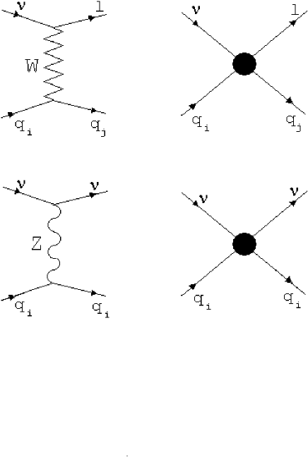
Figure 2: Feynman diagrams contributing to charged current and neutral current processes.

$${\cal M}^{\rm CC}=-\frac{ig^{2}}{2(Q^{2}+M_{W}^{2})}\bar{l}\gamma_{\mu}P_{L}\nu\medspace\bar{q}_{j}\gamma^{\mu}(g^{{}^{\prime}}_{L}P_{L}+g^{{}^{\prime}}_{R}P_{R})q_{i},$$ (7)

where

$$\begin{split}g^{{}^{\prime}}_{L}&=1-\dfrac{(Q^{2}+M_{W}^{2})}{\Lambda^{2}}\eta_{LL}\dfrac{g_{N}^{2}}{g^{2}}\\ \\ g^{{}^{\prime}}_{R}&=-\dfrac{(Q^{2}+M_{W}^{2})}{\Lambda^{2}}\eta_{LR}\dfrac{g_{N}^{2}}{g^{2}}\end{split}$$ (8)

include the new physics effects.

The differential cross section for charged currents reads

$$\begin{split}\frac{d\sigma^{\rm CC}}{dxdy}=\frac{G_{F}^{2}s}{\pi}\left(\frac{M_{W}^{2}}{(Q^{2}+M_{W}^{2})}\right)^{2}x[g^{{}^{\prime}2}_{L}(Q^{\rm CC}+(1-y)^{2}\bar{Q}^{\rm CC})\\ +g^{{}^{\prime}2}_{R}(\bar{Q}^{\rm CC}+(1-y)^{2}Q^{\rm CC})],\end{split}$$ (9)

where for an isoscalar target we have the quark distribution functions

$$\begin{split}Q^{\rm CC}(x,Q^{2})&=\dfrac{u_{v}(x,Q^{2})+d_{v}(x,Q^{2})}{2}+\dfrac{u_{s}(x,Q^{2})+d_{s}(x,Q^{2})}{2}\\ &+s_{s}(x,Q^{2})+b_{s}(x,Q^{2})\\ \\ \bar{Q}^{\rm CC}(x,Q^{2})&=\dfrac{u_{s}(x,Q^{2})+d_{s}(x,Q^{2})}{2}+c_{s}(x,Q^{2})+t_{s}(x,Q^{2})\end{split}$$ (10)

Similarly, the neutral current amplitude is

$${\cal M}^{\rm NC}=-\frac{ig^{2}}{2c_{W}(Q^{2}+M_{Z}^{2})}\bar{\nu}\gamma_{\mu}P_{L}\nu\medspace\bar{q}_{i}\gamma^{\mu}(g^{{}^{\prime}}_{L}P_{L}+g^{{}^{\prime}}_{R}P_{R})q_{i},$$ (11)

where $c_{W}=\cos\theta_{W}$ and

$$\begin{split}g^{{}^{\prime}i}_{L}=g^{i}_{L}-\frac{Q^{2}+M_{Z}^{2}}{\Lambda^{2}}c_{W}^{2}\eta_{LL}\frac{g_{LL}^{2}}{g^{2}}\\ g^{{}^{\prime}i}_{R}=g^{i}_{R}-\frac{Q^{2}+M_{Z}^{2}}{\Lambda^{2}}c_{W}^{2}\eta_{LR}\frac{g_{LR}^{2}}{g^{2}}\end{split}$$ (12)

include the new physics effects. Here, $g^{U}_{L}=1/2-2/3x_{W}$, $g^{D}_{L}=-1/2+1/3x_{w}$, $g^{U}_{R}=-2/3x_{W}$, and $g^{D}_{R}=1/3x_{W}$.

The neutral current differential cross section is then

$$\begin{split}\frac{d\sigma^{\rm NC}}{dxdy}=\frac{G_{F}^{2}s}{\pi}\left(\frac{M_{Z}^{2}}{(Q^{2}+M_{Z}^{2})}\right)^{2}\sum_{i=U,D}x[g^{`i2}_{L}(Q^{i}+(1-y)^{2}\bar{Q}^{i})\\ +g^{`i2}_{R}(\bar{Q}^{i}+(1-y)^{2}Q^{i})],\end{split}$$ (13)

where the corresponding parton distributions for a isoscalar target read

$$\begin{split}Q^{U}(x,Q^{2})=\dfrac{u_{v}(x,Q^{2})+d_{v}(x,Q^{2})}{2}+\dfrac{u_{s}(x,Q^{2})+d_{s}(x,Q^{2})}{2}\\ +c_{s}(x,Q^{2})+t_{s}(x,Q^{2})\\ Q^{D}(x,Q^{2})=\dfrac{u_{v}(x,Q^{2})+d_{v}(x,Q^{2})}{2}+\dfrac{u_{s}(x,Q^{2})+d_{s}(x,Q^{2})}{2}\\ +s_{s}(x,Q^{2})+b_{s}(x,Q^{2})\\ \bar{Q}^{U}(x,Q^{2})=\dfrac{u_{s}(x,Q^{2})+d_{s}(x,Q^{2})}{2}+c_{s}(x,Q^{2})+t_{s}(x,Q^{2})\\ \bar{Q}^{D}(x,Q^{2})=\dfrac{u_{s}(x,Q^{2})+d_{s}(x,Q^{2})}{2}+s_{s}(x,Q^{2})+b_{s}(x,Q^{2}).\end{split}$$

IV Results

In order to evaluate the impact of the observable $\alpha$ to bound new physics effects, we have estimated the corresponding uncertainties. For the number of events we have considered it as distributed according to a Poisson distribution and we have propagated onto the angle $\alpha$. The number of events $N$ as a function of $\alpha_{\rm SM}$ is

$$N=2\pi n_{\rm T}T\Delta E\sigma(E)\phi_{0}(E)\int_{0}^{\alpha_{\rm SM}}d\theta\sin\theta e^{-\sigma_{T}(E)\tau(\theta)}$$ (14)

where we have considered the effective volume for contained events for which a accurate and simultaneous determination of the muon energy and shower energy is possible. For IceCube it corresponds to the instrumented volume, roughly 1 km³, that implies a number of target nucleons $n_{\rm T}\simeq 6\times 10^{38}$. For $T$ we have taken an integration time of $15$ yr corresponding to the lifetime of the experiment.

To propagate the error on $N$ to obtain the one on $\alpha$, we note that

$$\Delta N=\dfrac{dN}{d\alpha}\Delta\alpha,$$ (15)

and dividing by $N$ we obtain for $\Delta\alpha$,

$$\Delta\alpha=\left[\int^{\alpha_{\rm SM}(E)}_{0}d\theta\left(\dfrac{\sin\theta}{\sin\alpha_{\rm SM}(E)}\right)e^{\sigma_{T}(E)[\tau(\alpha_{\rm SM}(E))-\tau(\theta)]}\right]\left(\dfrac{\Delta N}{N}\right),$$ (16)

where for Poisson distributed events we have

$$\Delta N=\sqrt{N}.$$ (17)

In the evaluation of the errors on $\alpha$ it is necessary to consider the initial flux $\phi_{0}^{\nu_{\mu}}$ to estimate the events rates.

The usual benchmark here is the so-called Waxman-Bahcall (WB) flux for each flavor,

$$E_{\nu_{\mu}}^{2}\phi_{WB}^{\nu_{\mu}}\simeq 2\times 10^{-8}{\rm GeV}\ {\rm cm}^{-2}{\rm s}^{-1}{\rm sr}^{-1},$$ (18)

which is derived assuming that neutrinos come from transparent cosmic ray sources waxman-bahcall , and that there is adequate transfer of energy to pions following $pp$ collisions. However, one should keep in mind that if there are in fact hidden sources which are opaque to ultra-high energy cosmic rays, then the expected neutrino flux will be higher.

On the other hand, we have the experimental bound set by AMANDA. A summary of the bounds can be found in Refs. desiati ; amanda-bound and a representative value for it is

$$E_{\nu_{\mu}}^{2}\phi_{AM}^{\nu_{\mu}}\simeq 2\times 10^{-7}{\rm GeV}\ {\rm cm}^{-2}{\rm s}^{-1}{\rm sr}^{-1}.$$ (19)

However, with the intention to estimate the number of events we have considered an intermediate flux level slightly below the present AMANDA experimental bound,

$$E_{\nu_{\mu}}^{2}\phi_{IN}^{\nu_{\mu}}\simeq 10^{-7}{\rm GeV}\ {\rm cm}^{-2}{\rm s}^{-1}{\rm sr}^{-1},$$ (20)

which is the flux that we have used to estimate the uncertainties on the angle $\alpha$.

In Fig. 3 we show our results for the $\alpha$ observable for the most representative sets of parameters and the standard model prediction, including the theoretical uncertainties from the SM cross section, the Earth density, and the errors coming from the statistical uncertainties in the number of events. For the new physics effects we have considered the sets of parameters shown in Table 1.

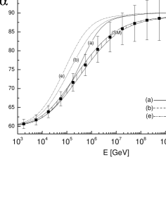
Figure 3: $\alpha(E)$ for different sets of parameters: (a) set1, (b) set2, (e) set5, and the standard model prediction with the theoretical uncertainties included (Shaded region) and the errors in $\alpha$ as resulting from the ones in the events numbers.

Table 1: Sets of parameters for the new four- fermion contact interactions.

Set	$\eta_{LL}$	$\eta_{LR}$	$\Lambda$ (TeV)
1	1	1	$1$
2	-1	-1	$1$
3	-1	-1	$2$
4	1	1	$0.8$
5	-1	-1	$0.8$

In Fig. 4 we show the differences between the values of $\alpha$ for different sets of parameters and the standard model values as a function of the energy. It can be seen that the maximum sensitivity is reached in the intermediate energy range ($10^{5}\rm{GeV}<E<10^{7}\rm{GeV}$). In this figure we also include the uncertainties in the Standard Model prediction coming from the ones in the event numbers (Shaded region).

In the same context, we can define another observable related to $\alpha_{\rm SM}(E)$. We consider the hemisphere $0<\theta<\pi/2$ divided into two regions by the angle $\alpha_{\rm SM}$, ${\cal R}_{1}$ for $0<\theta<\alpha_{\rm SM}$ and ${\cal R}_{2}$ for $\alpha_{\rm SM}<\theta<\pi/2$. We then calculate the ratio $\chi$ between the number of events for each region,

$$\chi=\frac{N_{1}}{N_{2}},$$ (21)

where $N_{1}$ is the number of events in the region ${\cal R}_{1}$ and $N_{2}$ is the number of events in the region ${\cal R}_{2}$. By using $\chi$, the effects of experimental systematics and initial flux dependence are also reduced.

If there is only standard model physics, then we have that the ratio $\chi=1$. The new physics effects produce a deviation from the standard value as we show in Fig. 5 for the different sets of parameters (different values of $\Lambda$, $\eta_{LL}$, and $\eta_{LR}$).

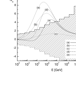
Figure 4: Differences between $\alpha$ for different sets of parameters and the standard model prediction ($\Delta_{\alpha}=\alpha_{\rm SM}-\alpha_{{\rm Set}_{i}}$). We have included the uncertainties on $\Delta_{\alpha}$ calculated for the intermediate initial flux $\phi_{IN}$ (Shaded region). The bin partition energy interval is taken as $\Delta\log_{10}E=0.5$

V Conclusions

In the present work we have studied a new observable that combines the surviving neutrino flux after passing through the Earth in a way that reduces the experimental systematics and the dependence with the initial flux. This observable, the angle $\alpha$, divides the upward-going hemisphere (with respect the arrival neutrino directions) into two homo-event sectors and it is dependent, of course, on the neutrino energy. The function $\alpha(E)$ is sharply dependent on the neutrino-nucleon cross section, which makes it a useful observable to bound new physics. In order to test the sensitivity of $\alpha$, we have calculated the new physics effects coming from four-fermion contact interactions. We have also studied as another observable, the ratio between the number of events in the regions defined by $\alpha_{\rm SM}(E)$.

We note that the introduced observable present no deviation from the standard model prediction for low energies ($<10^{3}$ GeV) at which almost no interactions occur with or without new physics. At high energies ($>10^{9}$ GeV) the neutrino mean free path is so small that the integrated surviving flux of Earth skimming neutrinos equals the one corresponding to almost the whole hemisphere. The corresponding increase in the cross section implies that, given the exponential behavior of the integrated flux, a great attenuation takes place both taking into account new physics effects or not.

Finally, we point out that this technique can be applied to any specific case of physics beyond the standard model, which is left for future work.

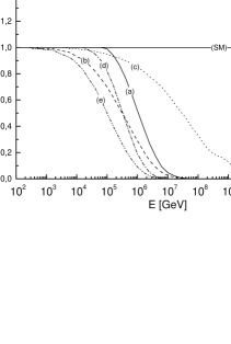
Figure 5: Observable $\chi(E)$ for different sets of parameters.

- (1) K. Mannheim, Astropart. Phys. 3, 295 (1996).
- (2) E. Waxman and J. Bahcall, Phys. Rev. Lett. 78, 2292 (1997).
- (3) IceCube Collaboration Astropart. Phys. 20, 507, (2004).
- (4) P. Jain, S. Kar, D. W. McKay, S. Panda, J. P. Ralston, Phys. ReV. D 66, 065018 (2002).
- (5) L. A. Anchordoqui, C. A. Garcia Canal, H. Goldberg, D. Gomez Dumm, F. Halzen, Phys. ReV. D 74, 125021 (2006).
- (6) J. Kwiecinski, A. D. Martin and A. M. Stasto, Phys. ReV. D 59, 093002 (1999).
- (7) N. Arteaga-Romero, C. Carimalo, A. Nicolaidis, O. Panella, G.Tsirigoti, Phys. Letter B 409, 299 (1997).
- (8) E. Waxman and J. N. Bahcall, Phys. Rev. D 59, 023002 (1999)
- (9) A. Nicolaidis and A. Taramopoulus, Phys. Lett. B 386, 211 (1996).
- (10) Luis A. Anchordoqui, Matthew M. Glenz and Leonard Parker, Phys. Rev.D75, 024011, (2007).
- (11) R. Gandhi, C. Quigg, M. H. Reno, I. Sarcevic, Astropart. Phys. 5 81:110 (1996).
- (12) A. M. Dziewonski and D. L. Anderson, Phys. Earth Planet Inter. 25, 297 (1981)
- (13) E.J.Eichten, K.D.Lane, M.E.Peskin, Phys. Lett. Lett. 50, 811 (1983).
- (14) P.Desiati, astro-ph/0611603
- (15) M.Ackermann et al, Astroparticle Physics 22, 339-353 (2005).