February 2007

The MSSM with large $\tan\beta$ and heavy squarks ($M_{\tilde{q}}\stackrel{{\scriptstyle>}}{{{}_{\sim}}}1$ TeV) is a theoretically well motivated and phenomenologically interesting extension of the SM. This scenario naturally satisfies all the electroweak precision constraints and, in the case of not too heavy slepton sector ($M_{\tilde{\ell}}\stackrel{{\scriptstyle<}}{{{}_{\sim}}}0.5$ TeV), can also easily accommodate the $(g-2)_{\mu}$ anomaly. Within this framework non-standard effects could possibly be detected in the near future in a few low-energy flavour-violating observables, such as ${\mathcal{B}}({B\to\tau\nu})$, ${\mathcal{B}}(B_{s,d}\to\ell^{+}\ell^{-})$, ${\mathcal{B}}(B\to X_{s}\gamma)$, and ${\mathcal{B}}(\mu\to e\gamma)$. Interpreting the $(g-2)_{\mu}$ anomaly as the first hint of this scenario, we analyse the correlations of these low-energy observables under the additional assumption that the relic density of a Bino-like LSP accommodates the observed dark matter distribution.

1 Introduction

Within the Minimal Supersymmetric extension of the Standard Model (MSSM), the scenario with large $\tan\beta$ and heavy squarks is a particularly interesting subset of the parameter space. On the one hand, values of $\tan\beta\sim$ 30–50 can allow the unification of top and bottom Yukawa couplings, as predicted in well-motivated grand-unified models [1]. On the other hand, heavy soft-breaking terms in the squark sector (both bilinear and trilinear couplings) with large $\tan\beta$ and a Minimal Flavour Violating (MFV) structure [2, 3] lead to interesting phenomenological virtues. On the one hand, this scenario can easily accommodate all the existing constraints from electroweak precision tests and flavour physics. In particular, in a wide region of the parameter space, the lighetst Higgs boson mass is above the present exclusion bound. On the other hand, if the slepton sector is not too heavy, within this framework one can also find a natural description of the present $(g-2)_{\mu}$ anomaly. In the near future, additional low-energy signatures of this scenario could possibly show up in ${\mathcal{B}}({B\to\tau\nu})$, ${\mathcal{B}}(B_{s,d}\to\ell^{+}\ell^{-})$, and ${\mathcal{B}}(B\to X_{s}\gamma)$ (see Ref. [4, 5] for a recent phenomenological discussion). In the parameter region relevant to $B$-physics and the $(g-2)_{\mu}$ anomaly, also a few Lepton Flavor Violating (LFV) processes (especially $\mu\to e\gamma$) are generally predicted to be within the range of upcoming experiments. In this paper we analyse the correlations of the most interesting low-energy observables of this scenario under the additional assumption that the relic density of a Bino-like lightest supersymmetric particle (LSP) accommodates the observed dark matter distribution (the constraints and reference ranges for the low-energy observables considered in this work can be found in Sect. 3.2).

Recent astrophysical observations consolidate the hypothesis that the universe is full of dark matter localized in large clusters [6]. The cosmological density of this type of matter is determined with good accuracy

$$0.079\leq\Omega_{\rm CDM}h^{2}\leq 0.119\quad\rm{at}\>2\sigma\>\rm{C.L.},$$ (1)

suggesting that it is composed by stable and weakly-interactive massive particles (WIMPs). As widely discussed in the literature (see e.g. Ref. [7] for recent reviews), in the MSSM with $R$-parity conservation a perfect candidate for such form of matter is the neutralino (when it turns out to be the LSP) [8]. In this scenario, due to the large amount of LSP produced in the early universe, the lightest neutralino must have a sufficiently large annihilation cross-section in order to satisfy the upper bound on the relic abundance.

If the $\mu$ term is sufficiently large (i.e. in the regime where the interesting Higgs-mediated effects in flavour physics are not suppressed) and $M_{1}$ is the lightest gaugino mass (as expected in a GUT framework), the lightest neutralino is mostly a Bino. Due to the smallness of its couplings, a Bino-like LSP tends to have a very low annihilation cross section. However, as we will discuss in Section 2, in the regime with large $\tan\beta$ and heavy squarks the relic-density constraints can easily be satisfied. In particular, the largest region of the parameter space yielding the correct LSP abundance is the so-called $A$-funnel region [9]. Here the dominant neutralino annihilation amplitude is the Higgs-mediated diagram in Fig. 1. Interestingly enough, in this case several of the parameters which control the amount of relic abundance, such as $\tan\beta$ and the heavy Higgs masses, also play a key role in flavour observables. As a result, in this scenario imposing the dark-matter constraints leads to a well-defined pattern of constraints and correlations on the low-energy observables which could possibly be tested in the near future. The main purpose of this article is the investigation of this scenario.

Figure 1: Higgs-mediated neutralino annihilation amplitude.

The interplay of $(g-2)_{\mu}$, ${\mathcal{B}}(B_{s,d}\to\ell^{+}\ell^{-})$, ${\mathcal{B}}(B\to X_{s}\gamma)$, and dark-matter constraints in the MSSM have been addressed in a series of recent works, focusing both on relic abundance [10] and on direct WIMPs searches [11]. Our analysis is complementary to those studies for two main reasons: i) the inclusion of ${\mathcal{B}}({B\to\tau\nu})$, which starts to play a significant role in the large $\tan\beta$ regime, and will become even more significant in the near future; ii) the study of a phenomenologically interesting region of the MSSM parameter space which goes beyond the scenarios analysed in most previous studies (see Section 2).

The plan of the paper is the following: in Section 2 we recall the ingredients to evaluate the relic density in the MSSM, and determine the key parameters of the interesting $A$ funnel region. In Section 3 we present a brief updated on the low-energy constraints on this scenario; we analyse constraints and correlations on the various low-energy observables after imposing the dark-matter constraints; we finally study the possible correlations between $(g-2)_{\mu}$ and the lepton-flavour violating decays ${\mathcal{B}}(\mu\to e\gamma)$ and ${\mathcal{B}}(\tau\to\mu\gamma)$. The results are summarized in the Conclusions.

2 Relic Density

In the following we assume that relic neutralinos represent a sizable fraction of the observed dark matter. In order to check if a specific choice of the MSSM parameters is consistent with this assumption, we need to ensure two main conditions: i) the LSP is a thermally produced neutralino; ii) its relic density is consistent with the astrophysical observation reported in Eq. (1).

In the MSSM there are four neutralino mass eigenstates, resulting from the admixture of the two neutral gauginos ($\tilde{W}^{0},\tilde{B}$) and the two neutral higgsinos ($\tilde{H}_{1}^{0},\tilde{H}_{2}^{0}$). The lightest neutralino can be defined by its composition,

$${\tilde{\chi}}_{1}=Z_{11}\tilde{B}+Z_{12}\tilde{W}^{0}+Z_{13}\tilde{H}_{1}^{0}+Z_{14}\tilde{H}_{2}^{0}$$ (2)

where the coefficients $Z_{1i}$ and the mass eigenvalue ($M_{{\tilde{\chi}}_{1}}$) are determined by the diagonalization of the mass matrix

$$\mathcal{M}_{{\tilde{\chi}}}=\left(\begin{array}[]{cccc}M_{1}&0&-m_{Z}\cos\beta\,s_{W}&m_{Z}\sin\beta\,s_{W}\\ 0&M_{2}&m_{Z}\cos\beta\,c_{W}&-m_{Z}\sin\beta\,c_{W}\\ -m_{Z}\cos\beta\,s_{W}&m_{Z}\cos\beta\,c_{W}&0&-\mu\\ m_{Z}\sin\beta\,s_{W}&-m_{Z}\sin\beta\,c_{W}&-\mu&0\end{array}\right).$$ (3)

As usual, $\theta_{W}$ denotes the weak mixing angle ($c_{W}\equiv\cos\theta_{W}$, $s_{W}\equiv\sin\theta_{W}$) and $\beta$ is defined by the relation $\tan\beta\equiv v_{2}/v_{1}$, where $v_{2(1)}$ is the vacuum expectation value of the Higgs coupled to up(down)-type quarks; $M_{1}$ and $M_{2}$ are the soft-breaking gaugino masses and $\mu$ is the supersymmetric-invariant mass term of the Higgs potential.

In order to compute the present amount of neutralinos we assume a standard thermal history of the universe [12] and evaluate the annihilation and coannihilation cross-sections using the micrOMEGAs [13] code. Since we cannot exclude other relic contributions in addition to the neutralinos, we have analysed only the consistency with the upper limit in Eq. (1). This can be translated into a lower bound on the neutralino cross sections: the annihilation and coannihilation processes have to be effective enough to yield a sufficiently low neutralino density at present time.

With respect to most of the existing analysis of dark-matter constraints in the MSSM, in this work we do not impose relations among the MSSM free parameters dictated by specific supersymmetry-breaking mechanisms. Consistently with the analysis of Ref. [4], we follow a bottom-up approach supplemented by few underlying hypothesis, such as the large value of $\tan\beta$ and the heavy soft-breaking terms in the squark sector. As far as the neutralino mass terms are concerned, we employ the following two additional hypotheses: the GUT relation $M_{1}\approx M_{2}/2\approx M_{3}/6$, and the relation $\mu>M_{1}$, which selects the parameter region with the most interesting Higgs-mediated effects in flavour physics (see Section 3). These two hypotheses imply that the lightest neutralino is Bino-like (i.e. $Z_{11}\gg Z_{1j\not=1}$) with a possible large Higgsino fraction when $\mu=\mathcal{O}(M_{1})$. Due to the smallness of the $\tilde{B}$ couplings, some enhancements of the annihilation and coannihilation processes are necessary in order to fulfill the relic density constraint. In general, these enhancements can be produced by the following three mechanisms [14, 7]:

• Light sfermions. For light sfermions, the $t$-channel sfermion exchange leads to a sufficiently large annihilation amplitude into fermions with large hypercharge.

• Coannihilation with other SUSY particles. If the next-to-lightest supersymmetric particle (NLSP) mass is closed to $M_{{\tilde{\chi}}_{1}}$, the coannihilation process NLSP+LSP $\to$ SM can be efficient enough to reduce the amount of neutralinos down to the allowed range. A relevant coannihilation process in our scenario occurs when the NLSP is the lightest stau lepton (stau annihilation region). This mechanism becomes relevant when the lightest stau mass, $M^{2}_{\tilde{\tau}_{R}}\approx M^{2}_{\tilde{\ell}}-m_{\tau}\mu\tan\beta$, satisfies the following condition

  $$M_{{\tilde{\chi}}_{1}}<M_{\tilde{\tau}_{R}}\stackrel{{\scriptstyle<}}{{{}_{\sim}}}1.1\times M_{{\tilde{\chi}}_{1}}~{}.$$ (4)

  Other relevent coannihilation processes take place when $\mu$ is sufficiently close to $M_{1}$. In this case the LSP coannihilation with a light neutralino or chargino (mostly higgsino-like and thus with mass $M_{{\tilde{\chi}}_{2}^{0},{\tilde{\chi}}_{1}^{+}}\sim\mu$), can become efficient.

• Resonant processes. Neutralinos can efficiently annihilate into down-type fermion pairs through $s$-channel exchange close to resonance (see Fig. 1). At large $\tan\beta$, the potentially dominant effect is through the heavy-Higgs exchange ($A$ and $H^{0}$) and in this case the resonant condition implies

  $$M_{{\tilde{\chi}}_{1}}\approx M_{A}/2~{}.$$ (5)

  At resonance the amplitude is proportional to $(M_{{\tilde{\chi}}_{1}}/M^{2}_{A})\,(Z_{11}Z_{13,14})(m_{b,\tau}/m_{W})\tan\beta$ which shows that the lightest neutralino must have a non-negligible higgsino component ($Z_{13,14}\not=0$), and that the annihilation into $b$ and $\tau$ fermions grows at large $\tan\beta$ (relaxing the resonance condition).

Because of the heavy squark masses, the first of these mechanisms is essentially excluded in the scenario we are considering: we assume squark masses in the $1-2$ TeV range and, in order to maintain a natural ratio between squark and slepton masses, this implies sleptons masses in the $0.3$–$1$ TeV range. The second mechanism can occur, but only in specific regions. On the other hand, the $s$-channel annihilation ${\tilde{\chi}}{\tilde{\chi}}\to H,A\to b\bar{b}(\tau^{+}\tau^{-})$ can be very efficient in a wide region of the parameter space of our scenario.

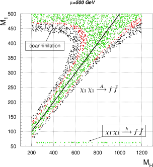
Figure 2: Allowed regions in the $M_{1}$–$M_{H}$ plane satisfying the relic density constraint $\Omega h^{2}<0.119$ for $M_{\tilde{q}}=2M_{\tilde{\ell}}=|A_{U}|=1$  TeV. Left panel: $\mu=0.5~{}{\rm TeV}$ with $\tan\beta=20$ (green), $30$ (green+red) and $50$ (all points up to $M_{1}\approx 480$ GeV, see right panel). Right panel: $\mu=0.5~{}{\rm TeV}$ (black) and $\mu=1~{}{\rm TeV}$ (blue) for $\tan\beta=50$ (a color version of this and the following figures can be found in the on-line version of this article).

In Fig. 2 we explore the dark-matter constraints in the $M_{1}$–$M_{H}$ plane, assuming heavy squarks and sleptons ($M_{\tilde{q}}=1$ TeV, $M_{\tilde{\ell}}=0.5$ TeV) and large trilinear couplings ($|A_{U}|=1$ TeV). The allowed points have been obtained for different values of $\mu$ and $\tan\beta$. The dependence on $\tan\beta$ at fixed $\mu$ ($\mu=0.5$ TeV) is illustrated by the left panel, while the $\mu$ dependence at fixed $\tan\beta$ ($\tan\beta=50$) is illustrated by the right panel. In all cases the heavy-Higgs resonant region, $M_{1}\approx M_{H,A}/2$, is the most important one. The $M_{H}$-independent regions for $M_{1}>450$ GeV and $M_{1}\sim 60$ GeV are generated by the ${\tilde{\chi}}$ coannihilation mechanisms and the $h$ resonance amplitude, respectively. As can be seen, in the heavy-Higgs resonant case the allowed region becomes larger for larger $M_{H}$ values: this is because the Higgs width grows with $M_{H}$ and therefore the resonance region becomes larger. For a similar reason, and also because the annihilation cross sections grow with $\tan\beta$, the allowed region becomes larger for larger $\tan\beta$ values. As far as the $\mu$ dependence is concerned, the heavy-Higgs resonance region is larger for small $\mu$ values. This is because the ${\tilde{\chi}}{\tilde{\chi}}A$ coupling, relevant in the resonant process, depends on the Higgsino component of ${\tilde{\chi}}$: for large $\mu$, ${\tilde{\chi}}$ is almost a pure $\tilde{B}$ and the ${\tilde{\chi}}{\tilde{\chi}}A$ coupling is suppressed. This fact can be used to set a theoretical upper limit on the $\mu$ parameter in this specific framework: $\mu$ must be larger than $M_{1}$ in order to reproduce a Bino LSP, but it should not be too heavy not to suppress too much the Bino annihilation amplitude.

Notice that in the right panel of Fig. 2 only the ${\tilde{\chi}}-\tilde{\tau}$ coannihilation process is active when $\mu=1~{}\rm{TeV}$. On general grounds, given a left-handed slepton mass $M_{\tilde{\ell}}$, the stau coannihilation region appears for lower $M_{1}$ if $\mu$ increases, since $M_{\tilde{\tau}}$ decreases with increasing $\mu$. Notice also that the $h$ resonance region disappears for large $\mu$, due to the smallness of the ${\tilde{\chi}}{\tilde{\chi}}h$ coupling. In both figures points with $M_{\tilde{\tau}}<M_{{\tilde{\chi}}_{1}}$ have not been plotted since they are ruled out.

In summary, the MSSM scenario we are considering is mainly motivated by flavour-physics and electroweak precision observables. As we have shown in this Section, in this framework the dark matter constraints can be easily fulfilled with a Bino-like LSP and an efficient Higgs-mediated Bino annihilation amplitude. The latter condition implies a strong link between the gaugino and the Higgs sectors (most notably via the relation $M_{1}\approx M_{H}/2$). This link reduces the number of free parameters, enhancing the possible correlations among low-energy observables.

3 Low-energy observables

In this Section we analyse the correlations of new-physics effects in $a_{\mu}=(g-2)_{\mu}/2$, ${\mathcal{B}}({B\to\tau\nu})$, ${\mathcal{B}}(B_{s,d}\to\ell^{+}\ell^{-})$, ${\mathcal{B}}(B\to X_{s}\gamma)$, ${\mathcal{B}}(\mu\to e\gamma)$, and ${\mathcal{B}}(\tau\to\mu\gamma)$, after imposing the dark matter constraints. As far as the $B$-physics observables are concerned, we use the existing calculations of supersymmetric effects in the large $\tan\beta$ regime which have been been recently reviewed in Ref. [4, 5]. However, since a few inputs have changed since then, most notably the ${\mathcal{B}}({B\to\tau\nu})$ measurements [22, 23] and the SM calculation of ${\mathcal{B}}(B\to X_{s}\gamma)$ [25], in the following we first present a brief updated on these two inputs. We then proceed analysing the implications on the MSSM parameter space of $a_{\mu}$ and $B$-physics observables after imposing the dark matter constraints. Finally, the possible correlations between $a_{\mu}$ and the lepton-flavour violating decays ${\mathcal{B}}(\mu\to e\gamma)$ and ${\mathcal{B}}(\tau\to\mu\gamma)$ in this framework are discussed.

3.1 Updated constraints from $B\to\tau\nu$ and $B\to X_{s}\gamma$

Due to its enhanced sensitivity to tree-level charged-Higgs exchange, [19] $B\to\tau\nu$ is one of the most clean probes of the large $\tan\beta$ scenario. The recent $B$-factory results [22, 23] ,

$${\cal B}({B\to\tau\nu})^{\rm Babar} = (0.88^{+0.68}_{-0.67}(\mbox{stat})\pm 0.11(\mbox{syst}))\times 10^{-4}~{},$$

$${\cal B}({B\to\tau\nu})^{\rm Belle} = (1.79^{+0.56}_{-0.49}(\mbox{stat})^{+0.46}_{-0.51}(\mbox{syst}))\times 10^{-4}~{},$$ (6)

leads to the average ${\cal B}({B\to\tau\nu})^{\rm exp}=(1.31\pm 0.49)\times 10^{-4}~{}$. This should be compared with the SM expectation ${\cal B}({B\to\tau\nu})^{\rm SM}=G_{F}^{2}m_{B}m_{\tau}^{2}f_{B}^{2}|V_{ub}|^{2}(1-m_{\tau}^{2}/m_{B}^{2})^{2}/(8\pi\Gamma_{B})$, whose numerical value suffers from sizable parametrical uncertainties induced by $f_{B}$ and $V_{ub}$. According to the global fit of Ref. [24], the best estimate is ${\cal B}({B\to\tau\nu})^{\rm SM}=(1.41\pm 0.33)\times 10^{-4}~{}$, which implies

$$R_{B\tau\nu}^{\rm exp}=\frac{{\mathcal{B}}^{\rm exp}({B\to\tau\nu})}{{\mathcal{B}}^{\rm SM}({B\to\tau\nu})}~{}=~{}0.93\pm 0.41~{}.$$ (7)

A similar (more transparent) strategy to minimize the error on ${\cal B}({B\to\tau\nu})^{\rm SM}$ is the direct normalization of ${\cal B}({B\to\tau\nu})$ to $\Delta M_{B_{d}}$, given that $B_{d}$–$\bar{B}_{d}$ is not affected by new physics in our scenario [4]. In this case, using $B_{B_{d}}(m_{b})=0.836\pm 0.068$ and $|V_{ub}/V_{td}|=0.473\pm 0.024$ [24], we get

$$\left(R^{\prime}_{B\tau\nu}\right)^{\rm exp} = \frac{{\mathcal{B}}^{\rm exp}({B\to\tau\nu})/\Delta M_{B_{d}}^{\rm exp}}{{\mathcal{B}}^{\rm SM}({B\to\tau\nu})/\Delta M_{B_{d}}^{\rm SM}}$$ (8)

$$= 1.27\pm 0.50~{}=~{}1.27\pm 0.48_{\rm exp}\pm 0.10_{|B_{B_{d}}|}\pm 0.13_{|V_{ub}/V_{td}|}~{},$$ (9)

in reasonable agreement with Eq. (7). Although perfectly compatible with 1 (or with no new physics contributions), these results leave open the possibility of $O(10\%-30\%)$ negative corrections induced by the charged-Higgs exchange. The present error on $R^{(\prime)}_{B\tau\nu}$ is too large to provide a significant constraint in the MSSM parameter space. In order to illustrate the possible role of a more precise determination of ${\mathcal{B}}^{\rm exp}({B\to\tau\nu})$, in the following we will consider the impact of the reference range $0.8<R_{B\tau\nu}<0.9$. In the next 2-3 years, at the end of the $B$-factory programs, we can expect a reduction of the experimental error on ${\cal B}({B\to\tau\nu})$ of a factor of 2-3. Depending on the possible shift of the central value of the measurement [note the large spread among the two central values in Eq. (6)] the upper bound $R_{B\tau\nu}<0.9$ could become the true 68% or 90% CL limit.

The $B\to X_{s}\gamma$ transition is particularly sensitive to new physics. However, contrary to ${B\to\tau\nu}$, it does not receive tree-level contributions from the Higgs sector. The one-loop charged-Higgs amplitude, which increases the rate compared to the SM expectation, can be partially compensated by the chargino-squark amplitude even for squark masses of $O(1~{}{\rm TeV})$. According to the recent NNLO analysis of Ref. [25], the SM prediction is

$${\cal B}(B\to X_{s}\gamma;E_{\gamma}>1.6~{}{\rm GeV})^{\rm SM}=(3.15\pm 0.23)\times 10^{-4}~{},$$ (10)

to be compared with the experimental average [26, 27, 28]

$${\cal B}(B\to X_{s}\gamma;E_{\gamma}>1.6~{}{\rm GeV}))^{\rm exp}=(3.55\pm 0.24)\times 10^{-4}~{}.$$ (11)

Combining these results, we obtain the following 1$\sigma$ CL interval

$$1.01<R_{Bs\gamma}=\frac{{\cal B}^{\rm exp}(B\to X_{s}\gamma)}{{\cal B}^{\rm SM}(B\to X_{s}\gamma)}<1.24$$ (12)

which will be used to constrain the MSSM parameter space in the following numerical analysis.

3.2 Combined constraints in the MSSM parameter space

The combined constraints from low-energy observables and dark matter in the $\tan\beta$–$M_{H}$ plane are illustrated in Figures 3 and 4. The plots shown in these figures have been obtained setting $M_{\tilde{q}}=1.5$ TeV, $|A_{U}|=1$ TeV, $\mu=0.5$ or $1$ TeV, and $M_{\tilde{\ell}}=0.4$ or $0.3$ TeV. The two sets of figures differ because of the sign of $A_{U}$. The gaugino masses, satisfying the GUT condition $M_{2}\approx 2M_{1}\approx M_{3}/3$, have been varied in each plot in order to fulfill the dark-matter conditions discussed in the previous Section (see Figure 2). These conditions cannot be fulfilled in the gray (light-blue) areas with heavy $M_{H}$, while the yellow band denotes the region where the stau coannihilation mechanism is active. The remaining bands correspond to the following constraints/reference-ranges from low-energy observables:

• $B\to X_{s}\gamma$ [$1.01<R_{Bs\gamma}<1.24$]: allowed region between the two blue lines.

• $a_{\mu}$ [$2<10^{9}(a_{\mu}^{\rm exp}-a_{\mu}^{\rm SM})<4$ [31]]: allowed region between the two purple lines.

• $B\to\mu^{+}\mu^{-}$ [${\cal B}^{\rm exp}<8.0\times 10^{-8}$ [32]]: allowed region below the dark-green line.

• $\Delta M_{B_{s}}$ [$\Delta M_{B_{s}}=17.35\pm 0.25~{}{\rm ps}^{-1}$ [33]]: allowed region below the gray line.

• $B\to\tau\nu$ [$0.8<R_{B\tau\nu}<0.9$]: allowed region between the two black lines [ red (green) area if all the other conditions (but for $a_{\mu}$) are satisfied].

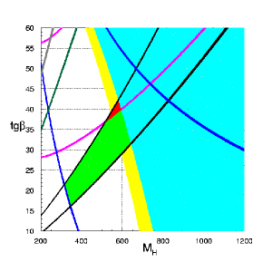
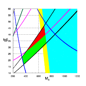
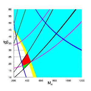
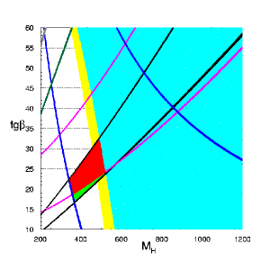
Figure 3: Combined constraints from low-energy observables and dark matter in the $\tan\beta$–$M_{H}$ plane. The plots have been obtained for $M_{\tilde{q}}=1.5$ TeV $A_{U}=-1$ TeV, and $[\mu,M_{\tilde{\ell}}]=[1.0,0.4]$ TeV (upper left); $[\mu,M_{\tilde{\ell}}]=[0.5,0.4]$ TeV (upper right); $[\mu,M_{\tilde{\ell}}]=[1.0,0.3]$ TeV (lower left); $[\mu,M_{\tilde{\ell}}]=[0.5,0.3]$ TeV (lower right). The light-blue area is excluded by the dark-matter conditions. Within the red (green) area all the reference values of the low-energy observables (but for $a_{\mu}$) are satisfied. See main text for more details. The yellow band denote the area where the stau coannihilation mechanism is active ($1<M_{\tilde{\tau}_{R}}/M_{\tilde{B}}<1.1$); in this area the $A$-funnel region and the stau coannihilation region overlap.

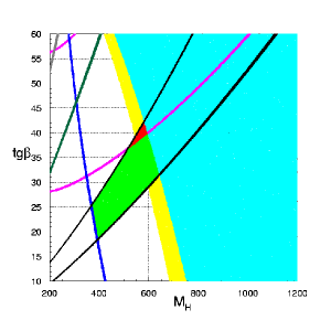
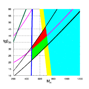
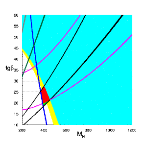
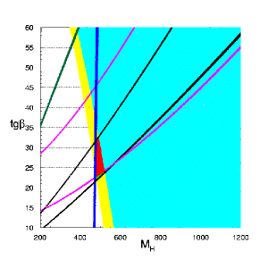
Figure 4: Same notations and conventions as in Figure 3, but for $A_{U}=1$ TeV.

In the excluded regions at large $M_{H}$ (light-blue areas) the neutralino cannot satisfy the resonance condition $M_{{\tilde{\chi}}_{1}}\approx M_{H}/2$ and, at the same time, be lighter than the sleptons. This is why the excluded regions become larger for lighter $M_{\tilde{\ell}}$. For the same reason, the excluded regions become larger for larger values of $\mu$ (we recall that $M^{2}_{\tilde{\tau}_{R}}\approx M^{2}_{\tilde{\ell}}-m_{\tau}\mu\tan\beta$). We stress that in all cases we have explicitly checked the consistency with electroweak precision tests and the compatibility with exclusion bounds on direct SUSY searches. By construction, these conditions turn out to be naturally satisfied in the scenarios we have considered. The mot delicate constraint is the value of the lightest Higgs boson mass ($m_{h}$), which lies few GeV above its exlusion bound. In particular, we find 118 GeV $\leq m_{h}\leq$ 120 GeV in the plots of Figure 3, and 117 GeV $\leq m_{h}\leq$ 119 GeV in Figure 4.

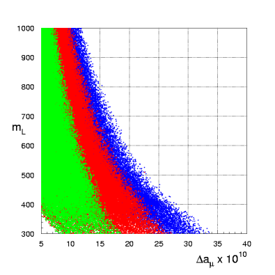
Figure 5: $\Delta a_{\mu}=(g_{\mu}-g^{\rm SM}_{\mu})/2$ vs. the slepton mass within the funnel region taking into account the $B\to X_{s}\gamma$ constraint and setting $R_{B\tau\nu}>0.7$ (blue), $R_{B\tau\nu}>0.8$ (red), $R_{B\tau\nu}>0.9$ (green). The supersymmetric parameters have been varied in the following ranges: 200 GeV $\leq M_{2}\leq$ 1000 GeV, 500 GeV $\leq\mu\leq$ 1000 GeV, $10\leq\tan\beta\leq 50$. Moreover, we have set $A_{U}=-1$ TeV, $M_{\tilde{q}}=1.5~{}$TeV, and imposed the GUT relation $M_{1}\approx M_{2}/2\approx M_{3}/6$.

As can be seen, in Figure 3 the $B\to X_{s}\gamma$ constraint is always easily satisfied for $M_{H}\stackrel{{\scriptstyle>}}{{{}_{\sim}}}300$ GeV, or even lighter $M_{H}$ values for large $\tan\beta$ values. This is because the new range in Eq. (12) allows a significant (positive) non-standard contribution to the $B\to X_{s}\gamma$ rate. Moreover, having chosen $A_{U}<0$, the positive charged-Higgs contribution is partially compensated by the negative chargino-squarks amplitude. In Figure 4, where $A_{U}>0$, the $B\to X_{s}\gamma$ constraints are much more stringent and almost $\tan\beta$-independent. It is worth noting that in Figure 3 the $B\to X_{s}\gamma$ information also exclude a region at large $M_{H}$: this is where the chargino-squarks amplitude dominates over the charged-Higgs one, yielding a total negative corrections which is not favored by data. As already noted in [4], the precise $\Delta M_{B_{s}}$ measurement and the present limit on $B\to\mu^{+}\mu^{-}$ do not pose any significant constraint.

A part from the excluded region at large $M_{H}$, the most significant difference with respect to the analysis of Ref. [4] (where dark-matter constraints have been ignored) is the interplay between $a_{\mu}$ and $B$-physics observables. The correlation between $M_{1}$ and $M_{H}$ imposed by the dark matter constraint is responsible for the rise with $M_{H}$ of the $a_{\mu}$ bands in Figures 3 and 4. This makes more difficult to intercept the $B\to X_{s}\gamma$ and ${B\to\tau\nu}$ bands and, as a result, only a narrow area of the parameter space can fulfill all constraints. In particular, with the reference ranges we have chosen, the best overlap occurs for moderate/large values of $\tan\beta$ and low values of $\mu$ and $M_{\tilde{\ell}}$.

On the other hand, we recall that the ${B\to\tau\nu}$ band in Figure 3 does not correspond to the present experimental determination of this observable, but only to an exemplifying range. Assuming a stronger suppression of ${\mathcal{B}}({B\to\tau\nu})$ with respect to its SM value would allow a larger overlap between the $B\to X_{s}\gamma$ and ${B\to\tau\nu}$ bands in the regions with higher values of $\tan\beta$, $\mu$ and $M_{\tilde{\ell}}$. While if the ${\mathcal{B}}({B\to\tau\nu})$ measurement will converge toward the SM value, for the reference values of $\mu$ and $M_{\tilde{\ell}}$ chosen in the figures ($\mu\geq 0.5$ GeV, $M_{\tilde{\ell}}\geq 0.3$ GeV) we deduce that: i) for $R_{B\tau\nu}>0.8$ the non-standard contribution to $a_{\mu}$ cannot not exceed $3\times 10^{-9}$; ii) for $R_{B\tau\nu}>0.9$ the non-standard contribution to $a_{\mu}$ cannot not exceed $2\times 10^{-9}$. An illustration of how the non-standard contribution to $a_{\mu}$ varies as a funtion of $M_{\tilde{\ell}}$, imposing different bounds on $R_{B\tau\nu}$, is shown in Figure 5. Moreover, if the ${\mathcal{B}}({B\to\tau\nu})$ measurement will converge toward the SM value and the $a_{\mu}$ constraint is not considered, the green areas in Figures 3 and 4 are enlarged, allowing also lower $\tan\beta$ values.

In short, the main result of this analysis is that in a scenario with heavy squarks and large trilinear couplings, the constraints and reference ranges for the low-energy observables described above favor a charged Higgs mass in the $400-600$ GeV range and $\tan\beta$ values in the 20-40 range. The structure of the favored $\tan\beta-M_{H}$ region depends on other SUSY parameters, mainly $\mu$ and $M_{\tilde{\ell}}$. Lower slepton masses shift the region toward lower $M_{H}$ and lower $\tan\beta$ values (in order to reproduce the $(g-2)_{\mu}$ anomaly and a neutralino LSP), while large $\mu$ values reduce the favored region selecting larger $M_{H}$ and $\tan\beta$ values.

The analysis of future phenomenological signals of this scenario at LHC and other experiments is beyond the scope of this work. However it should be noticed that both squarks and gluinos are rather heavy (around or above $1$ TeV) and therefore not easily detectable. On the other hand, a direct detection of the charged Higgs and/or of the sleptons should be possible. In this case, the combination of high-energy and low-energy observables would allow to determine the $\tan\beta$ parameter very precisely.

3.3 Correlation between LFV decays and $(g-2)_{\mu}$

As we have seen from the analysis of Figures 3 and 4, a key element which characterizes the scenario we are considering is the interplay between $(g-2)_{\mu}$ and $B$-physics observables. Since $(g-2)_{\mu}$ is affected by irreducible theoretical uncertainties [31], it is desirable to identify additional observables sensitive to the same (or a very similar) combination of supersymmetric parameters. An interesting possibility is provided by the LFV transitions $\ell_{i}\rightarrow\ell_{j}\gamma$ and, in particular, by the $\mu\rightarrow e\gamma$ decay. Apart from the unknown overall normalization associated to the LFV couplings, the amplitude of these transitions are closely connected to those generating the non-standard contribution to $a_{\mu}$ [34].

LFV couplings naturally appear in the MSSM once we extend it to accommodate the non-vanishing neutrino masses and mixing angles by means of a supersymmetric seesaw mechanism [35]. In particular, the renormalization-group-induced LFV entries appearing in the left-handed slepton mass matrices have the following form [35]:

$$\delta_{LL}^{ij}~{}=~{}\frac{\left(M^{2}_{\tilde{\ell}}\right)_{L_{i}L_{j}}}{\sqrt{\left(M^{2}_{\tilde{\ell}}\right)_{L_{i}L_{i}}\left(M^{2}_{\tilde{\ell}}\right)_{L_{j}L_{j}}}}=c_{\nu}(Y^{\dagger}_{\nu}Y_{\nu})_{ij}~{},$$ (13)

where $Y_{\nu}$ are the neutrino Yukawa couplings and $c_{\nu}$ is a numerical coefficient, depending on the SUSY spectrum, typically of ${\cal O}(0.1$–$1)$. As is well known, the information from neutrino masses is not sufficient to determine in a model-independent way all the seesaw parameters relevant to LFV rates and, in particular, the neutrino Yukawa couplings. To reduce the number of free parameters specific SUSY-GUT models and/or flavour symmetries need to be employed. Two main roads are often considered in the literature (see e.g. Ref. [36] and references there in): the case where the charged-lepton LFV couplings are linked to the CKM matrix (the quark mixing matrix) and the case where they are connected to the PMNS matrix (the neutrino mixing matrix). These two possibilities can be formulated in terms of well-defined flavour-symmetry structures starting from the MFV hypothesis [37, 38]. A useful reference scenario is provided by the so-called MLFV hypothesis [37], namely by the assumption that the flavour degeneracy in the lepton sector is broken only by the neutrino Yukawa couplings, in close analogy to the quark sector. According to this hypothesis, the LFV entries introduced in Eq. (13) assume the following form

$$\delta_{LL}^{ij}~{}=~{}c_{\nu}(Y^{\dagger}_{\nu}Y_{\nu})_{ij}~{}\approx~{}c_{\nu}\displaystyle\frac{m_{\nu}^{\rm atm}M_{\nu_{R}}}{v_{2}^{2}}~{}U_{i3}U^{*}_{j3}$$ (14)

where $M_{\nu_{R}}$ is the average right-handed neutrino mass and $U$ denote the PMNS matrix.

Once non-vanishing LFV entries in the slepton mass matrices are generated, LFV rare decays are naturally induced by one-loop diagrams with the exchange of gauginos and sleptons (gauge-mediated LFV amplitudes). In particular, the leading contribution due to the exchange of charginos, leads to

$$\frac{{\mathcal{B}}(\ell_{i}\rightarrow\ell_{j}\gamma)}{{\mathcal{B}}(\ell_{i}\rightarrow\ell_{j}\nu_{\ell_{i}}\bar{\nu_{\ell_{j}}})}=\frac{48\pi^{3}\alpha}{G_{F}^{2}}\left|\frac{\alpha_{2}}{4\pi}\left(\frac{\mu M_{2}}{m^{2}_{L}}\right)\frac{f_{2c}\left(M^{2}_{2}/M^{2}_{\tilde{\ell}},\mu^{2}/M^{2}_{\tilde{\ell}}\right)}{(M_{2}^{2}\!-\!\mu^{2})}\,\delta_{LL}^{ij}\tan\beta,\right|^{2}$$ (15)

where the loop function $f_{2c}(x,y)$ is defined as $f_{2c}(x,y)=f_{2c}(x)-f_{2c}(y)$ in terms of

$$f_{2c}(a)=\frac{-a^{2}-4a+5+2(2a+1)\ln a}{2(1-a)^{4}}\,.$$ (16)

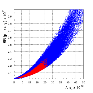
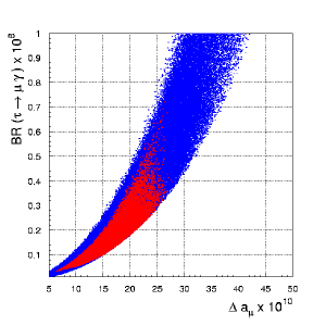
Figure 6: Expectations for ${\mathcal{B}}(\mu\rightarrow e\gamma)$ and ${\mathcal{B}}(\tau\rightarrow\mu\gamma)$ vs. $\Delta a_{\mu}=(g_{\mu}-g^{\rm SM}_{\mu})/2$, assuming $|\delta_{LL}^{12}|=10^{-4}$ and $|\delta_{LL}^{23}|=10^{-2}$. The plots have been obtained employing the following ranges: 300 GeV $\leq M_{\tilde{\ell}}\leq$ 600 GeV, 200 GeV $\leq M_{2}\leq$ 1000 GeV, 500 GeV $\leq\mu\leq$ 1000 GeV, $10\leq\tan\beta\leq 50$, and setting $A_{U}=-1$ TeV, $M_{\tilde{q}}=1.5~{}$TeV. Moreover, the GUT relations $M_{2}\approx 2M_{1}$ and $M_{3}\approx 6M_{1}$ are assumed. The red areas correspond to points within the funnel region which satisfy the $B$-physics constraints listed in Section 3.2 [${\mathcal{B}}(B_{s}\rightarrow\mu^{+}\mu^{-})<8\times 10^{-8}$, $1.01<R_{Bs\gamma}<1.24$, $0.8<R_{B\tau\nu}<0.9$, $\Delta M_{B_{s}}=17.35\pm 0.25~{}{\rm ps}^{-1}$].

Given that both $\ell_{i}\rightarrow\ell_{j}\gamma$ and $\Delta a_{\mu}=(g_{\mu}-g^{\rm SM}_{\mu})/2$ are generated by dipole operators, it is natural to establish a link between them. To this purpose, we recall the dominant contribution to $\Delta a_{\mu}$ is also provided by the chargino exchange and can be written as

$$\Delta a_{\mu}=-\frac{\alpha_{2}}{4\pi}m_{\mu}^{2}\left(\frac{\mu M_{2}}{m_{L}^{2}}\right)\frac{g_{2c}\left(M^{2}_{2}/M^{2}_{\tilde{\ell}},\mu^{2}/M^{2}_{\tilde{\ell}}\right)}{(M_{2}^{2}\!-\!\mu^{2})}\tan\beta\,,$$ (17)

with $g_{c2}(x,y)$ defined as $f_{c2}(x,y)$ in terms of

$$g_{c2}(a)=\frac{(3-4a+a^{2}+2\log a)}{(a-1)^{3}}~{}.$$ (18)

It is then straightforward to deduce the relation

$$\frac{{\mathcal{B}}(\ell_{i}\rightarrow\ell_{j}\gamma)}{{\mathcal{B}}(\ell_{i}\rightarrow\ell_{j}\nu_{\ell_{i}}\bar{\nu_{\ell_{j}}})}=\frac{48\pi^{3}\alpha}{G_{F}^{2}}\left[\frac{\Delta a_{\mu}}{m_{\mu}^{2}}\right]^{2}\,\left[\frac{f_{2c}\left(M^{2}_{2}/M^{2}_{\tilde{\ell}},\mu^{2}/M^{2}_{\tilde{\ell}}\right)}{g_{2c}\left(M^{2}_{2}/M^{2}_{\tilde{\ell}},\mu^{2}/M^{2}_{\tilde{\ell}}\right)}\right]^{2}\,\left|\delta_{LL}^{ij}\right|^{2}~{}.$$ (19)

To understand the relative size of the correlation, in the limit of degenerate SUSY spectrum we get

$${\mathcal{B}}(\ell_{i}\rightarrow\ell_{j}\gamma)~{}\approx~{}\left[\frac{\Delta a_{\mu}}{20\times 10^{-10}}\right]^{2}\times\left\{\begin{array}[]{ll}1\times 10^{-4}\,\left|\delta_{LL}^{12}\right|^{2}&[\mu\to e]~{},\\ 2\times 10^{-5}\,\left|\delta_{LL}^{23}\right|^{2}&[\tau\to\mu]~{}.\end{array}\right.$$ (22)

A more detailed analysis of the stringent correlation between the $\ell_{i}\rightarrow\ell_{j}\gamma$ transitions and $\Delta a_{\mu}$ in our scenario is illustrated in Fig.6. Since the loop functions for the two processes are not identical, the correlation is not exactly a line; however, it is clear that the two observables are closely connected. We stress that the numerical results shown in Fig.6. have been obtained using the exact formulae reported in Ref. [39] for the supersymmetric contributions to both ${\mathcal{B}}(\ell_{i}\rightarrow\ell_{j}\gamma)$ and $\Delta a_{\mu}$ (the simplified results in the mass-insertion approximations in Eqs. (15)–(19) have been shown only for the sake of clarity). The red areas are the regions where the $B$-physics constraints are fulfilled. In our scenario the $B$-physics constraints put a lower bound on $M_{H}$ and therefore, through the funnel-region relation, also on $M_{1,2}$ (see Figs. 3 and 4). As a result, the allowed ranges for $\Delta a_{\mu}$ and ${\mathcal{B}}(\ell_{i}\rightarrow\ell_{j}\gamma)$ are correspondingly lowered. A complementary illustration of the interplay of $B$ physics observables, dark-matter constraints, $\Delta a_{\mu}$, and LFV rates –within our scenario– is shown in Figure 7.

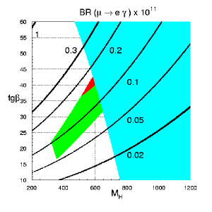
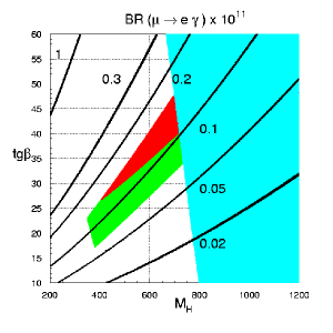
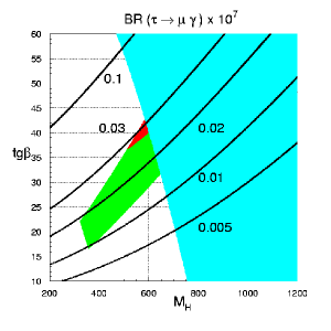
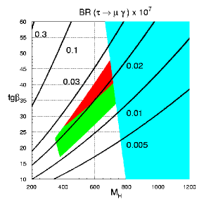
Figure 7: Isolevel curves for ${\mathcal{B}}(\mu\rightarrow e\gamma)$ and ${\mathcal{B}}(\tau\rightarrow\mu\gamma)$ assuming $|\delta_{LL}^{12}|=10^{-4}$ and $|\delta_{LL}^{23}|=10^{-2}$ in the $\tan\beta$–$M_{H}$ plane. The green/red areas correspond to the allowed regions for the low-energy observables illustrated in Figure 3 for $[\mu,M_{\tilde{\ell}}]=[1.0,0.4]$ TeV (left plots), $[\mu,M_{\tilde{\ell}}]=[0.5,0.4]$ TeV (right plots).

Observable	Exp. bound	Bound on	Expected $|\delta_{LL}|$ in MLFV
		the eff coupl.	for $M_{\nu_{R}}=10^{12}$ GeV
${\mathcal{B}}(\mu\to e\,\gamma)$	$<1.2\times 10^{-11}$	$|\delta_{LL}^{21}|<3\times 10^{-4}$	$(0.3-3)\times 10^{-4}$
${\mathcal{B}}(\tau\to e\,\gamma)$	$<1.1\times 10^{-7}$	$|\delta_{LL}^{31}|<8\times 10^{-2}$	$(0.3-3)\times 10^{-4}$
${\mathcal{B}}(\tau\to\mu\,\gamma)$	$<6.8\times 10^{-8}$	$|\delta_{LL}^{32}|<6\times 10^{-2}$	$0.8\times 10^{-3}$

Table 1: Present experimental bounds on the radiative LFV decays of $\tau$ and $\mu$ leptons [40] and corresponding bounds on the effective LFV couplings $\delta^{ij}_{LL}$. The bounds are obtained by means of Eq. (19) setting $\Delta a_{\mu}=20\times 10^{-10}$. The expectations for the $\delta^{ij}_{LL}$ reported in the last two columns correspond to MLFV ansatz in Eq. (14) with $c_{\nu}=1$ and $M_{\nu_{R}}=10^{12}$ GeV.

The normalization $|\delta_{LL}^{12}|=10^{-4}$ used in Figures 6 and 7 corresponds to the central value in Eq. (14) for $c_{\nu}=1$ and $M_{\nu_{R}}=10^{12}$ GeV. This normalization can be regarded as a rather natural (or even pessimistic) choice. As can be seen from Figures 6 and 7, for such natural choice of $\delta_{LL}$ the $\mu\rightarrow e\gamma$ branching ratio is in the $10^{-12}$ range, i.e. well within the reach of MEG [42] experiment. Note that this is a well-defined prediction of our scenario, where the connection between $\mu\rightarrow e\gamma$ and $\Delta a_{\mu}$ allows us to substantially reduce the number of free parameters. In particular, the requirement of a supersymmetric contribution to $\Delta a_{\mu}$ of $O(10^{-9})$ forces a relatively light sparticle spectrum and moderate/large $\tan\beta$ values which both tend to enhance the LFV rates. This fact already allows to exclude values of $\delta_{LL}^{12}$ above $10^{-3}$, for which ${\mathcal{B}}(\mu\rightarrow e\gamma)$ would exceed the present experimental bound. Within the MLFV hypothesis, this translates into a non-trivial upper bound on the right-handed neutrino mass: $M_{\nu_{R}}<10^{13}$ GeV.

On the other hand, the normalization $|\delta_{LL}^{23}|=10^{-2}$ adopted for the $\tau\to\mu\gamma$ mode is more optimistic given the MLFV expectations in Table 1. We have chosen this reference value because only for such large LFV entries the $\tau\to\mu\gamma$ transition could be observed in the near future. From the comparison of Figure 6 and Table 1 we deduce that, unless $\mu\to e\gamma$ is just below its present exclusion bound, an observation of $\tau\to\mu\gamma$ above $10^{-9}$ would exclude the LFV pattern predicted by the MLFV hypothesis [37].

4 Conclusions

Within the wide parameter space of the supersymmetric extensions of the SM, the regime of large $\tan\beta$ and heavy squarks represents an interesting corner. It is a region consistent with present data, where the $(g-2)_{\mu}$ anomaly and the upper bound on the Higgs boson mass could find a natural explanation. Moreover, this region could possibly be excluded or gain more credit with more precise data on a few $B$-physics observables, such as ${\mathcal{B}}({B\to\tau\nu})$ and ${\mathcal{B}}(B\to\ell^{+}\ell^{-})$. In this paper we have analysed the correlations of the most interesting low-energy observables within this scenario, interpreting the $(g-2)_{\mu}$ anomaly as the first hint of this scenario, and assuming that the relic density of a Bino-like LSP accommodates the observed dark matter distribution. In view of improved experimental searches of LFV decays, we have also analysed the expectations for the rare decays $\mu\to e\gamma$ and $\tau\to\mu(e)\gamma$ in this framework.

The main conclusions of our analysis can be summarised as follows:

• Within this region it is quite natural to fulfill the dark-matter constraints thanks to the resonance enhancement of the ${\tilde{\chi}}_{1}{\tilde{\chi}}_{1}\to H,A\to f\bar{f}$ cross section ($A$-funnel region). As shown in Fig. 2, this mechanism is successful in a sufficiently wide area of the parameter space.

• From the phenomenological point of view, the most significant impact of the dark-matter constraints is the non-trivial interplay between $a_{\mu}$ and the $B$-physics observables. A supersymmetric contribution to $a_{\mu}$ of ${\cal O}(10^{-9})$ is perfectly compatible with the present constraints from ${\mathcal{B}}(B\to X_{s}\gamma)$, especially for $A_{U}<0$. However, taking into account the correlation between neutralino and charged-Higgs masses occurring in the $A$-funnel region, this implies a sizable suppression of ${\mathcal{B}}({B\to\tau\nu})$ with respect to its SM prediction. As shown in Figure 5, the size of this suppression depends on the slepton mass, which in turn controll the size of the supersymmetric contribution to $a_{\mu}$. In particular, we find that $\Delta a_{\mu}\stackrel{{\scriptstyle>}}{{{}_{\sim}}}2\times 10^{-9}$ implies a relative suppression of ${\mathcal{B}}({B\to\tau\nu})$ larger than $10\%$ A more precise determination of ${\mathcal{B}}({B\to\tau\nu})$ is therefore a key element to test this scenario.

• A general feature of supersymmetric models is a strong correlation between $\Delta a_{\mu}$ and the rate of the LFV transitions $\ell_{i}\rightarrow\ell_{j}\gamma$ [34]. We have re-analysed this correlation in our framework, taking into account the updated constraints on $\Delta a_{\mu}$ and $B$-physics observables, and employing the MLFV ansatz [37] to relate the flavour-violating entries in the slepton mass matrices to the observed neutrino mass matrix. According to the latter (pessimistic) hypothesis, we find that the $\mu\rightarrow e\gamma$ branching ratio is likely to be within the reach of MEG [42] experiment, while LFV decays of the $\tau$ leptons are unlikely to exceed the $10^{-9}$ level.

References

- [1] G. Anderson, S. Raby, S. Dimopoulos, L. J. Hall and G. D. Starkman, Phys. Rev. D 49 (1994) 3660 [hep-ph/9308333]; T. Blazek, R. Dermisek and S. Raby, Phys. Rev. D 65 (2002) 115004 [hep-ph/0201081].
- [2] L. J. Hall and L. Randall, Phys. Rev. Lett. 65 (1990) 2939.
- [3] G. D’Ambrosio, G. F. Giudice, G. Isidori and A. Strumia, Nucl. Phys. B645 (2002) 155.
- [4] G. Isidori and P. Paradisi, Phys. Lett. B 639 (2006) 499 [hep-ph/0605012].
- [5] E. Lunghi, W. Porod and O. Vives, Phys. Rev. D 74 (2006) 075003 [hep-ph/0605177].
- [6] D. N. Spergel et al. [WMAP Collab.], astro-ph/0603449.
- [7] J. R. Ellis, K. A. Olive, Y. Santoso and V. C. Spanos, Phys. Lett. B 565 (2003) 176 [hep-ph/0303043]; G. Bertone, D. Hooper and J. Silk, Phys. Rept. 405 (2005) 279 [hep-ph/0404175], S. Profumo and C. E. Yaguna, Phys. Rev. D 70 (2004) 095004 [hep-ph/0407036].
- [8] H. Goldberg, Phys. Rev. Lett. 50 (1983) 1419; J. R. Ellis, J. S. Hagelin, D. V. Nanopoulos, K. A. Olive and M. Srednicki, Nucl. Phys. B 238 (1984) 453.
- [9] J. R. Ellis, L. Roszkowski and Z. Lalak, Phys. Lett. B 245 (1990) 545; J. L. Lopez, D. V. Nanopoulos and K. J. Yuan, Nucl. Phys. B 370 (1992) 445; M. Drees and M. M. Nojiri, Phys. Rev. D 47 (1993) 376 [hep-ph/9207234].
- [10] R. Dermisek, S. Raby, L. Roszkowski and R. Ruiz de Austri, JHEP 0509, 029 (2005) [hep-ph/0507233]; J. R. Ellis, K. A. Olive, Y. Santoso and V. C. Spanos, JHEP 0605 (2006) 063 [hep-ph/0603136].
- [11] S. Baek, Y. G. Kim and P. Ko, JHEP 0502 (2005) 067 [hep-ph/0406033]; S. Baek, D. G. Cerdeno, Y. G. Kim, P. Ko and C. Munoz, JHEP 0506 (2005) 017 [hep-ph/0505019]; Y. Mambrini, C. Munoz, E. Nezri and F. Prada, JCAP 0601 (2006) 010 [hep-ph/0506204].
- [12] E. W. Kolb and M. S. Turner, The Early universe, Front. Phys. 69 (1990) 1.
- [13] G. Belanger, F. Boudjema, A. Pukhov and A. Semenov, Comput. Phys. Commun. 176 (2007) 367 [hep-ph/0607059]; ibid. 149 (2002) 103 [hep-ph/0112278].
- [14] H. Baer et al., JHEP 0207, 050 (2002) [hep-ph/0205325]; U. Chattopadhyay, A. Corsetti and P. Nath, Phys. Rev. D 68 (2003) 035005 [hep-ph/0303201].
- [15] C. Hamzaoui, M. Pospelov and M. Toharia, Phys. Rev. D 59 (1999) 095005 [hep-ph/9807350]; C. S. Huang, W. Liao and Q. S. Yan, Phys. Rev. D 59 (1999) 011701 [hep-ph/9803460].
- [16] K. S. Babu and C. Kolda, Phys. Rev. Lett. 84 (2000) 228 [hep-ph/9909476]; G. Isidori and A. Retico, JHEP 0111, 001 (2001) [hep-ph/0110121].
- [17] A. J. Buras, P. H. Chankowski, J. Rosiek and L. Slawianowska, Nucl. Phys. B 619 (2001) 434 [hep-ph/0107048]; Nucl. Phys. B 659 (2003) 3 [hep-ph/0210145].
- [18] G. Degrassi, P. Gambino and G. F. Giudice, JHEP 0012 (2000) 009 [hep-ph/0009337]; M. Carena, D. Garcia, U. Nierste and C. E. Wagner, Phys. Lett. B B499 (2001) 141 [hep-ph/0010003].
- [19] W. S. Hou, Phys. Rev. D 48 (1993) 2342.
- [20] T. Moroi, Phys. Rev. D 53 (1996) 6565 [hep-ph/9512396]; S. P. Martin and J. D. Wells, Phys. Rev. D 64 (2001) 035003 [hep-ph/0103067].
- [21] A. Freitas, E. Gasser and U. Haisch, hep-ph/0702267.
- [22] B. Aubert et al. [BaBaR Collab.], hep-ex/0608019.
- [23] K. Ikado et al. [Belle Collab.], hep-ex/0604018.
- [24] M. Bona et al. [UTfit Collab.], JHEP 0610, 081 (2006) [hep-ph/0606167].
- [25] M. Misiak et al., hep-ph/0609232.
- [26] E. Barberio et al. [Heavy Flavor Averaging Group (HFAG)], hep-ex/0603003.
- [27] P. Koppenburg et al. [Belle Collab.], Phys. Rev. Lett. 93 (2004) 061803 [hep-ex/0403004].
- [28] B. Aubert et al. [BaBar Collab.], Phys. Rev. Lett. 97 (2006) 171803 [hep-ex/0607071].
- [29] T. Becher and M. Neubert, Phys. Rev. Lett. 98 (2007) 022003 [hep-ph/0610067].
- [30] E. Lunghi and J. Matias, hep-ph/0612166.
- [31] K. Hagiwara, A. D. Martin, D. Nomura and T. Teubner, hep-ph/0611102; M. Passera, Nucl. Phys. Proc. Suppl. 155 (2006) 365 [hep-ph/0509372].
- [32] M. Rescigno, talk presented at CKM Workshop 2006 (12–16 December 2006, Nagoya, Japan, http://ckm2006.hepl.phys.nagoya-u.ac.jp/); R. Bernhard et al. [CDF Collab.], hep-ex/0508058.
- [33] A. Abulencia et al. [CDF - Run II Collab.], Phys. Rev. Lett. 97 (2006) 062003 [AIP Conf. Proc. 870 (2006) 116] [hep-ex/0606027].
- [34] J. Hisano and K. Tobe, Phys. Lett. B 510 (2001) 197 [hep-ph/0102315].
- [35] F. Borzumati and A. Masiero, Phys. Rev. Lett. 57, 961 (1986);
- [36] A. Masiero, S. K. Vempati and O. Vives, Nucl. Phys. B 649, 189 (2003) [hep-ph/0209303]; New J. Phys. 6, 202 (2004) [hep-ph/0407325]; L. Calibbi, A. Faccia, A. Masiero and S. K. Vempati, Phys. Rev. D 74 (2006) 116002 [hep-ph/0605139].
- [37] V. Cirigliano, B. Grinstein, G. Isidori and M. B. Wise, Nucl. Phys. B 728, 121 (2005) [hep-ph/0507001].
- [38] B. Grinstein, V. Cirigliano, G. Isidori and M. B. Wise, Nucl. Phys. B 763 (2007) 35 [hep-ph/0608123].
- [39] J. Hisano, T. Moroi, K. Tobe, M. Yamaguchi and T. Yanagida, Phys. Lett. B 357 (1995) 579 [hep-ph/9501407].
- [40] W. M. Yao et al. [Particle Data Group], J. Phys. G 33 (2006) 1 [hppt://pdg.lbl.gov].
- [41] R. Barbieri and L. J. Hall, Phys. Lett. B 338 (1994) 212 [hep-ph/9408406]; R. Barbieri, L. J. Hall and A. Strumia, Nucl. Phys. B 445 (1995) 219 [hep-ph/9501334].
- [42] M. Grassi [MEG Collaboration], Nucl. Phys. Proc. Suppl. 149 (2005) 369.
- [43] K. S. Babu and C. Kolda, Phys. Rev. Lett. 89 (2002) 241802 [hep-ph/0206310].
- [44] P. Paradisi, JHEP 0602, 050 (2006) [hep-ph/0508054]; P. Paradisi, JHEP 0608, 047 (2006) [hep-ph/0601100].
- [45] A. Masiero, S. Profumo, S. K. Vempati and C. E. Yaguna, JHEP 0403 (2004) 046 [hep-ph/0401138].
- [46] P. Paradisi, JHEP 0510 (2005) 006 [hep-ph/0505046].