TTP07-05
SFB/CPP-07-07
DESY 07-024

Two-Loop Formfactors in Theories with Mass Gap
and $Z$-Boson Production

Abstract

The two-loop formfactor both for a $U(1)\times U(1)$ and a $SU(2)\times U(1)$ gauge theory with massive and massless gauge bosons respectively is evaluated at arbitrary momentum transfer $q^{2}$. The asymptotic behaviour for $q^{2}\to\infty$ is compared to a recent calculation of Sudakov logarithms. The result is an important ingredient for the calculation of radiative corrections to $Z$-boson production at hadron and lepton colliders.

1 Introduction

Precise measurements of cross sections for the production of massive and massless gauge bosons were one of the central topics of LEP experiments. At the LHC similar reactions, namely the production of $W$ and $Z$-bosons, singly or in pairs, with or without additional quark or gluon jets, will be crucial for precise studies of the electroweak and strong interactions. Single $W$- and $Z$-boson production will be used for the determination of parton distributions and eventually even for luminosity calibrations. A future linear collider, operating in the GIGA-$Z$ mode, will measure the properties of the $Z$-resonance with unprecedented precision. All these measurements will rely on the theoretical knowledge of radiative corrections to better than one percent accurracy, perhaps even down to the level of several permille. QCD and electroweak radiative corrections, as well as their interplay, thus will be crucial for the interpretation of these results.

QCD corrections to single $W$- and $Z$-production are identical to those for the Drell–Yan process and have been evaluated in two-loop approximation in [1, 2], those for Higgs boson production in [3]. Electroweak corrections for the on-shell process were computed some time ago (see e.g. [4] and references therein). The next step evidently requires to combine QCD and electroweak effects, resulting in non-factorizable terms of order $\alpha_{\rm weak}\alpha_{s}$. For the inclusive $Z$ decay rate these terms have been calculated for final states with up-, down-, and bottom-quarks [5, 6, 7] and turned out to be relevant for the precise determination of the strong coupling constant. However, these results cannot be directly applied to the production process and to more differential distributions. For the $Z$-boson such corrections for high $p_{T}$ distribution have been obtained in [8].

In the present paper we describe conceptial developments and concrete results which are important ingredients for the complete evaluation of these non-factorizable terms of order $\alpha_{\rm weak}\alpha_{s}$. In particular we consider those amplitudes which correspond to vertex diagrams with a virtual gluon attached to one-loop electroweak corrections. These are relevant for the “mixed” corrections of order $\alpha_{\rm weak}\alpha_{s}$ to $Z$-boson production, and for hadronic $Z$ decay. Essentially the same diagrams are also important ingredients for the combination of photonic and weak corrections to $Z$ production in electron-positron collisions and to leptonic $Z$ decays.

Our study identifies the infrared singular as well as the finite parts, investigates the structure of these singularities and shows how they can be combined with real radiation to arrive at a finite result. The infrared finite remainder will be presented in analytical form in terms of generalized polylogarithms.

The form factor will also be investigated in the Sudakov limit $M^{2}/q^{2}\ll 1$. In the special case of an Abelian theory the result coincides with the one of [9] (see also [10]) and allows to contrast the logarithmic approximation with the complete result. The calculational method relies on an approach that has already been successfully employed in a number of cases [11, 12]. General considerations restrict the structure of the final result to a sum of “basis functions” (in our case—generalized “harmonic” polylogarithms up to fourth degree) with specific arguments and prefactors. Calculating on one hand directly a large number of terms in the low $q^{2}$ expansion with the technique of large mass expansion, expanding the basis functions on the other hand, and equating the results, the coefficients in front of the basis functions can be determined. In a final step most of the basis functions are transformed into Nielsen polylogarithms, leading to a fairly compact result whose asymptotic behaviour can be analyzed in a straightforward manner.

To facilitate the discussion, we present, in a first step, in section 2, the results for a $U(1)\times U(1)$ theory with one of the gauge bosons taken to be massive, the other one massless. The explicit analytical result confirms the factorization of the infrared singularities and allows to identify the infrared-finite remainder. In section 3 the formalism will be extended to a massive nonabelian theory and applied to the complete set of virtual corrections of order $\alpha_{\rm weak}\alpha_{s}$, contributing to $Z$-boson production and decay. The triple-boson coupling leads to additional diagrams with additional generalized polylogarithms, which cannot easily be transformed into Nielson’s polylogarithms. However, they can be evaluated numerically with high precision [13] and their asymptotic behaviour is under control. The paper concludes with a brief summary. Much of the formulae and calculational details will be collected in the Appendices.

2 Abelian Theory

For definiteness and simplicity we will, in a first step, consider the form factor in a ficticious $U(1)\times U(1)$ theory with one massive and one massless gauge boson and with coupling constants $\alpha$ and $\alpha^{\prime}$ respectively.

For the Abelian theory the form factor $F$ will be defined as matrix element of an external current

$$\gamma_{\mu}F(q,M)=\int dxe^{-ixq}\langle\psi^{\prime}|J_{\mu}(x)|\psi\rangle.$$ (1)

Here $\psi$ and $\psi^{\prime}$ denote on-shell massless fermions of momenta $p$ and $p^{\prime}=p+q$, respectively, $M$ the mass of the gauge boson.

In a perturbative expansion

$$F(\alpha,\alpha^{\prime},q,M,\varepsilon)=\sum_{m,n=0}^{\infty}\left(\frac{\alpha}{4\pi}\right)^{m}\left(\frac{\alpha^{\prime}}{4\pi}\right)^{n}f^{(m,n)}(q,M,\varepsilon)$$ (2)

one needs to evaluate the expansion coefficients $f^{(m,n)}$. In Born and one-loop approximation they are given by

$$f^{(0,0)} = 1\,,$$ (3)

$$f^{(1,0)} = -\frac{7}{2}-\frac{2}{z}+\frac{2+3z}{z}\log(-z)+\frac{2(1+z)^{2}}{z^{2}}\Big{(}{\rm Li}_{2}(1+z)-\frac{\pi^{2}}{6}\Big{)}\,,$$ (4)

$$f^{(0,1)} = \left(\frac{\bar{\mu}^{2}}{-q^{2}}\right)^{\varepsilon}\left(-\frac{2}{\varepsilon^{2}}-\frac{3}{\varepsilon}-8+\zeta_{2}+\varepsilon\Big{(}-16+\frac{3}{2}\zeta_{2}+\frac{14}{3}\zeta_{3}\Big{)}\right)\,,$$ (5)

where $z=q^{2}/M^{2}+i0$, $\zeta_{n}=\zeta(n)$ is the Riemann $\zeta$-function and the infrared singularities are controlled by dimensional regularization in $d=4-2\varepsilon$ dimensions. In the euclidean region $q^{2}<0$, so that no imaginary parts appear in the above formulae.

The two-loop result for the massless case, $f^{(0,2)}$, can be found e.g. in [14, 15]. The two-loop result for the fully massive case, $f^{(2,0)}$, is only known in the large $q^{2}$ limit [16]. The evaluation of the mixed corrections is drastically simplified by the fact that the infrared singularities factorize within infrared evolution equation approach [17, 16], which gives in our case

$$F(\alpha,\alpha^{\prime},q^{2}/M^{2},\varepsilon)=F_{\rm massless}(\alpha^{\prime},q,\varepsilon)\tilde{F}(\alpha,\alpha^{\prime},q^{2}/M^{2})\,,$$ (6)

with $F_{\rm massless}=\sum(\alpha^{\prime}/4\pi)^{n}f^{(0,n)}(q,\varepsilon)$ denoting the formfactor for the massless theory and $\tilde{F}$ being free from infrared singularities. The function $\tilde{F}$ can again be expressed as double series, and the coefficients depend on the ratio $z=q^{2}/M^{2}$ only. The terms $\tilde{F}^{(m,0)}=f^{(m,0)}$ coincide by definition with those valid for the massive $U(1)$-theory. The evaluation of the nonfactorizable part of the two-loop contribution

$$\tilde{F}^{(1,1)}\equiv\phi(q^{2}/M^{2})$$ (7)

will be the central result of this section.

The Feynman diagrams necessary for this computation have two thresholds: at $q^{2}=0$ and at $q^{2}=M^{2}$. The analytical structure of vertex diagrams of this type has been explored in [11]. The coefficients of an expansion in $q^{2}/M^{2}$ (and $M^{2}/q^{2}$) can always be expressed as combinations of so-called harmonic sums [18] or more generally — nested harmonic sums [19]. These sums correspond to (generalized) polylogarithms ([20]) [21] of arguments $\pm q^{2}/M^{2}$ and their generalizations — harmonic polylogarithms [22] (see also [23]). This structure suggests the following method for the evaluation of Feynman integrals. First, using the method of large mass expansion [24], one calculates a large number of coefficients of the series in $q^{2}/M^{2}$. From the basis functions (polylogarithms) one then constructs an Ansatz with unknown coefficients $x_{i}$. Equating Ansatz and series one obtains a unique answer for parameters $x_{i}$. This method has been applied earlier [25, 11] to various scalar vertex masterintegrals. (In a different context the method has also been applied in [26]). Here it is applied to amplitudes deduced from a a set of realistic Feynman diagrams representing a physical process and leading to amplitudes with irreducible numerators and shrunken lines.

A few comments on this procedure are in order. First, the main problem is to write down the correct prefactors in the Ansatz. Empirically one finds that the presence of a numerator or the absence of a line may lead to the additional factors $M^{2}/q^{2}$ or $(M^{2}/q^{2})^{2}$ in front of polylogarithms. Therefore such factors should also be included in the Ansatz. Second, only five functions could not be represented as Nielsen polylogarithms with the argument $q^{2}/M^{2}$. These remaining functions belong to the class of harmonic polylogarithms [22] discussed in more detail in the Appendix.

Instead of expanding the amplitude in $q^{2}/M^{2}$ one could find the differential equation (see [27]) for a diagram and again apply an Ansatz based on polylogarithms. This approach has recently been used for similar two-loop vertex diagrams in [28].

Altogether 16 one-particle-irreducible two-loop vertex diagrams contribute to the formfactor. These diagrams can be obtained from the one-loop one shown in Fig. 1a by adding one gluon line. The two-loop, one-particle reducible diagrams which are obviously products of one-loop diagrams contribute to the term $\alpha\alpha^{\prime}f^{(0,1)}f^{(1,0)}$ and are not repeated here. We also do not display the contributions to the fermionic wave function renormalization, which receives contributions from additional 6 diagrams. For the generation of the input the program DIANA [29] has been used, for the evaluation and expansion a program written in FORM [30]. The evaluation of the Dirac traces has lead to about 700 different integrals. For most of them the asymptotic expansion was performed up to order 45 which required in total several hours of CPU time on a Pentium IV processor. For the remaining, most complicated cases (nonplanar diagram) up to 60 expansion coefficients had to be computed. For this purpose the parallel version of FORM [31], running on an SGI machine with multiprocessor SMP architecture, was used.

The function $\phi(z)$ can be cast into the following form (here and below $z=q^{2}/M^{2}+i0$)

$$\phi(z) = \frac{(1+z)^{2}}{z^{2}}\Biggl{(}(6L^{2}+24\zeta_{2}-24\zeta_{3})\log(1+z)+(-4L^{2}-6L-20\zeta_{2})\log^{2}(1+z)$$ (8)

$$+\frac{8}{3}\log^{3}(1+z)L+8\log^{2}(1+z){\rm Li}_{2}(-z)-12\log(1+z){\rm Li}_{2}(-z)$$

$$-16\log(1+z){\rm Li}_{3}(-z)+16\log(1+z){\rm S}_{1,2}(-z)-16{\rm Li}_{2}(-z)\zeta_{2}-4{\rm Li}_{2}(-z)L^{2}$$

$$-8{\rm Li}_{2}^{2}(-z)+16{\rm Li}_{3}(-z)L-24{\rm Li}_{4}(-z)-12{\rm S}_{1,2}(-z)+16{\rm S}_{1,2}(-z)L+16{\rm S}_{1,3}(-z)$$

$$-16{\rm S}_{2,2}(-z)+24h(z)-48H_{3}(z)+8H_{2}(z)+32H_{4}(z)\Biggr{)}$$

$$+\frac{1+3z+z^{2}}{z^{2}}\Biggl{(}-32{\rm Li}_{2}(z)\zeta_{2}-8{\rm Li}_{2}(z)L^{2}-8{\rm Li}_{2}(z){\rm Li}_{2}(z)+32{\rm Li}_{3}(z)L$$

$$-48{\rm Li}_{4}(z)+32{\rm S}_{2,2}(z)\Biggr{)}+\frac{1-z^{2}}{z^{2}}\Biggl{(}72\log(1-z)\zeta_{2}+18\log(1-z)L^{2}$$

$$+36\log(1-z){\rm Li}_{2}(z)+36{\rm Li}_{2}(z)L+72{\rm S}_{1,2}(z)\Biggr{)}+\frac{2+3z}{z}(32\zeta_{2}+12\zeta_{3})$$

$$-\frac{34+51z}{z}L+\frac{16+23z}{z}L^{2}-\frac{2(1-z)(13+27z)}{z^{2}}\log(1-z)+\frac{4(3+4z)}{z^{2}}{\rm Li}_{2}(-z)L$$

$$-\frac{2(1+z)(3+5z)}{z^{2}}\Bigl{(}\log(1+z)L+{\rm Li}_{2}(-z)\Bigr{)}+\frac{4(11+9z)}{z}{\rm Li}_{2}(z)$$

$$-\frac{4(3+2z-3z^{2})}{z^{2}}{\rm Li}_{3}(-z)-\frac{4(9+4z-6z^{2})}{z^{2}}{\rm Li}_{3}(z)+\frac{2(8-z)}{z},$$

where $L=\log(-q^{2}/M^{2})$, $\zeta_{a}=\zeta(a)$ is the Riemann $\zeta$-function, $S_{a,b}(z)$ are Nielsen polylogarithms [20]. The functions $h(z)$ and $H_{j}(z)$ are defined and discussed in Appendix A.

3 $Z$-Production

For definitenes and simplicity, consider, in the next step, $Z$-boson production in quark-antiquark annihilation. To fix the notation, we recapitulate the one-loop results. The weak corrections to the Born term can be split into those involving the exchange of $W$- and $Z$-bosons, (Fig.1(a)) and those involving the triple-boson coupling (Fig.1(b)). The combination of photonic and QCD corrections follows essentially from the two-loop QED or QCD results and will not be addressed here.

For a light quark the form factor can be decomposed as follows

$$F(q^{2})_{\mu}=\gamma_{\mu}\frac{1+\gamma_{5}}{2}F_{R}(q^{2})+\gamma_{\mu}\frac{1-\gamma_{5}}{2}F_{L}(q^{2})\,.$$ (9)

At the Born level the expressions for the form factors $F_{R}$ and $F_{L}$ are given by

$$F_{R}=i\frac{e}{s_{W}}g_{R}\,,\,\,\,F_{L}=i\frac{e}{s_{W}}g_{L}\,,$$ (10)

with $g_{R}=-Qs_{W}^{2}/c_{W}$ and $g_{L}=(I_{3}-Qs_{W}^{2})/c_{W}$ being the right- and left- handed couplings of a quark to the $Z$-boson. Here $I_{3}$ is the third component of the isospin of a quark, $Q$ its electric charge and $s_{W}=\sin\theta_{W}$ and $c_{W}=\cos\theta_{W}$ denote sine and cosine of the weak mixing angle, respectively.

Including radiative corrections and adopting a form similar to eq.6 the formfactors can be cast into the following form

$$F_{R} = i\frac{e}{s_{W}}\Big{(}1+C_{F}\frac{\alpha_{s}}{4\pi}f^{(0,1)}\Big{)}\Bigg{[}g_{R}+\frac{\alpha}{4\pi s_{W}^{2}}g_{R}^{3}\rho_{\rm A}(q^{2}/m_{Z}^{2},m_{Z}^{2})+C_{F}\frac{\alpha_{s}}{4\pi}\frac{\alpha}{4\pi s_{W}^{2}}g_{R}^{3}\phi_{\rm A}(q^{2}/m_{Z}^{2})\Bigg{]}\,,$$

$$F_{L} = i\frac{e}{s_{W}}\Big{(}1+C_{F}\frac{\alpha_{s}}{4\pi}f^{(0,1)}\Big{)}\Bigg{[}g_{L}$$ (11)

$$+ \frac{\alpha}{4\pi s_{W}^{2}}\Bigg{(}g_{L}^{3}\rho_{\rm A}(q^{2}/m_{Z}^{2},m_{Z}^{2})+\frac{g_{L}}{2}\rho_{\rm A}(q^{2}/m_{W}^{2},m_{W}^{2})+c_{W}\frac{I_{3}}{2}\rho_{\rm NA}(q^{2}/m_{W}^{2},m_{W}^{2})\Bigg{)}$$

$$+ C_{F}\frac{\alpha_{s}}{4\pi}\frac{\alpha}{4\pi s_{W}^{2}}\Bigg{(}g_{L}^{3}\phi_{A}(q^{2}/m_{Z}^{2})+\frac{g_{L}}{2}\phi_{\rm A}(q^{2}/m_{W}^{2})+c_{W}\frac{I_{3}}{2}\phi_{\rm NA}(q^{2}/m_{W}^{2})\Bigg{)}\Bigg{]}\,,$$

where first factors in the brackets in the above equations represent the QCD corrections. Terms given by $\rho_{\rm A}$ and $\rho_{\rm NA}$ account for the one-loop electroweak corrections. The abelian part $\rho_{\rm A}$ is defined by the diagram of the abelian type (Fig. 1a) and obviously closely related to $f^{(1,0)}$ defined in eq.4. The unrenormalized result is given by

$$\rho_{\rm A}(z,M^{2})=\frac{1}{\varepsilon}-\ln(M^{2}/\bar{\mu}^{2})-4-\frac{2}{z}+\frac{2+3z}{z}\log(-z)+\frac{2(1+z)^{2}}{z^{2}}\Big{(}{\rm Li}_{2}(1+z)-\frac{\pi^{2}}{6}\Big{)}\,.$$ (12)

The nonabelian part $\rho_{\rm NA}(z,M_{2})$ receives corrections from both diagrams of Fig.1a and Fig.1b. It is given by

$$\rho_{\rm NA}(z,M^{2}) = -2\rho_{\rm A}(z,M^{2})-2\Lambda(z,M^{2})\,,$$ (13)

$$\Lambda(z,M^{2}) = -\frac{3}{\varepsilon}+3\ln(M^{2}/\bar{\mu}^{2})-2+\frac{2}{z}-\Big{(}1+\frac{2}{z}\Big{)}\sqrt{1-\frac{4}{z}}\,l-\Big{(}1+\frac{1}{2z}\Big{)}\frac{4}{z}l^{2}$$ (14)

with

$$l=\ln\left(\frac{\sqrt{1-4/z}+1+i0}{\sqrt{1-4/z}-1+i0}\right)\,.$$ (15)

The function $\Lambda(z)$ can be taken from [33] (see also [34, 35, 36] and references therein for one-loop calculations in the Standard Model). We do not include the terms from the renormalization of the coupling and the $Z$-boson wave function which follow from textbook prescriptions and will not be considered in this work.

Evaluated for arbitrary $q^{2}\neq M_{Z}^{2}$, the above results are gauge dependent and are presented in Feynman gauge. For the offshell case they can be considered as building blocks for a complete calculation.

The functions $\phi_{\rm A}(z)$ and $\phi_{\rm NA}(z)$, representing the non-factorizable terms of $\cal{O}(\alpha\alpha_{s})$, are written in a form completely analogous to the electroweak one-loop terms. The function $\phi_{\rm A}(z)$ has been given in the previous section. The nonabelian part $\phi_{\rm NA}(z)$ involves new functions — generalized polylogarithms.

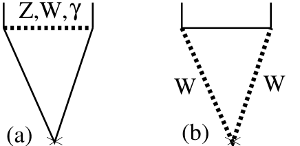
Figure 1: Diagrams, contributing to the vertex $Zq\bar{q}$ (a) and (b). The two-loop diagrams are obtained by attaching one virtual gluon in all possible ways. The case (b) represents nonabelian part. That gives contribution $\phi_{\rm NA}(z)$ in the text. Diagram (a) with $W$ exchange also contributes to $\phi_{\rm NA}(z)$.

Our result in Feynman gauge reads

$$\phi_{\rm A}(z) = \phi(z)\,,$$ (16)

$$\phi_{\rm NA}(z) = -2\phi_{\rm A}(z)$$ (17)

$$+4\frac{8-5z}{z}+48\frac{1+2z}{z^{2}}H_{0,-r,-r,-1}(-z)-12H_{-r,-r,-1}(-z)+8H_{0,-r,-r}(-z)$$

$$+4\frac{6+2z-3z^{2}}{z^{2}}H_{-r,-r}(-z)-6\frac{(4-z)(4+3z)}{z^{2}}gH_{-r,-1}(-z)$$

$$-2\frac{(4-z)(6+7z)}{z^{2}}gH_{-r}(-z)+\frac{16+23z}{z}\Bigl{(}8\zeta_{2}+2L^{2}\Bigr{)}-4\frac{12-11z^{2}}{z^{2}}{\rm Li}_{3}(z)$$

$$+2\frac{66+49z}{z}{\rm Li}_{2}(z)-4\frac{(1-z)(13+34z)}{z^{2}}\log(1-z)-16\frac{5+9z}{z}L$$

$$+\frac{(1-z^{2})}{z^{2}}\Biggl{(}96\log(1-z)\zeta_{2}+24\log(1-z)L^{2}$$

$$\qquad\qquad\qquad\qquad\qquad+48\log(1-z){\rm Li}_{2}(z)+48{\rm Li}_{2}(z)L+96{\rm S}_{1,2}(z)\Biggr{)}$$

$$+\frac{(1+4z+z^{2})}{z^{2}}\Biggl{(}-32{\rm Li}_{2}(z)\zeta_{2}-8{\rm Li}_{2}(z)L^{2}-8{\rm Li}_{2}^{2}(z)$$

$$\qquad\qquad\qquad\qquad\qquad+32{\rm Li}_{3}(z)L-48{\rm Li}_{4}(z)+32{\rm S}_{2,2}(z)\Biggr{)}\,.$$

The function $\phi_{\rm NA}(z)$ receives contributions not only from digrams of Fig. 1(b) but also from those of Fig. 1(a) with the exchange of $W$-boson. The functions $H_{\dots}$ are considered in more detail in Appendix B. For the special case $q^{2}=M^{2}$ one finds

$$\phi_{\rm A}(1+i0) = 14+72\zeta_{2}l_{2}-64\zeta_{2}l_{2}^{2}-\frac{16}{3}l_{2}^{4}+22\zeta_{2}-28\zeta_{3}+16\zeta_{4}-128{\rm Li}_{4}({\textstyle\frac{1}{2}})$$ (18)

$$+i\pi(85+32l_{2}+24l_{2}^{2}-\frac{32}{3}l_{2}^{3}+14\zeta_{2}-120\zeta_{3})$$

$$= -2.1073-19.0331i\,,$$ (19)

$$\phi_{\rm NA}(1+i0) = -16-144\zeta_{2}l_{2}+128\zeta_{2}l_{2}^{2}+\frac{32}{3}l_{2}^{4}+\frac{70}{3}\zeta_{2}+\frac{184}{3}\zeta_{3}-236\zeta_{4}$$ (20)

$$+26\frac{\pi}{\sqrt{3}}+256{\rm Li}_{4}({\textstyle\frac{1}{2}})-84\frac{1}{\sqrt{3}}{\rm Ls}_{2}({\textstyle\frac{\pi}{3}})-\frac{16}{3}\pi{\rm Ls}_{2}({\textstyle\frac{\pi}{3}})+96\Bigl{(}{\rm Ls}_{2}({\textstyle\frac{\pi}{3}})\Bigr{)}^{2}$$

$$+i\pi(54-64l_{2}-48l_{2}^{2}+\frac{64}{3}l_{2}^{3}-28\zeta_{2}+48\zeta_{3})$$

$$= -7.5880+16.7194i\,,$$ (21)

with $l_{2}=\log 2$. Substituting the actual masses of the $W$- and $Z$-bosons ($z=m_{Z}^{2}/m_{W}^{2}=1.2856$) we find:

$$\phi_{\rm A}(1.2856+i0) = -1.3598-30.4095i\,,$$ (22)

$$\phi_{\rm NA}(1.2856+i0) = -10.1248+35.0336i\,.$$ (23)

In the limit $q^{2}\to\infty$ the function $\phi$, as given by Eq. (8) coincides with the result of [9] where the power unsupressed logarithmic and constant part have been evaluated. For the leading and the first power suppressed term we find

$$\phi(z) = (3-24\zeta_{2}+48\zeta_{3})\log(-z)-2+40\zeta_{2}-84\zeta_{3}+14\zeta_{4}$$ (24)

$$+ \frac{1}{z}\bigg{(}(-26+8\zeta_{2})\log^{2}(-z)+(-120-16\zeta_{2}+128\zeta_{3})\log(-z)$$

$$\quad-188-8\zeta_{2}-8\zeta_{3}+116\zeta_{4}\bigg{)}+{\cal O}\left(\frac{1}{z^{2}}\right)$$

In Fig. 2 the exact result is compared with the Sudakov approximation and with the approximation including the first power-suppressed term. For electroweak interactions the mass of the gauge boson can be taken to be of order 100 GeV, the characteristic energy of order one to two TeV. For one TeV the relative error of the Sudakov approximation (the logarithmic plus constant term) amounts to 15%, at 2TeV it is reduced to 2.5%.

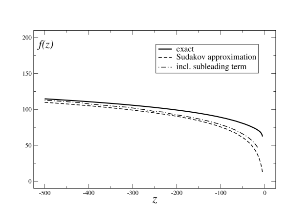
Figure 2: Non-factorizable two-loop correction to the abelian formfactor in the euclidean regime ($z=q^{2}/m^{2}$). The solid line represents the exact result, the dashed line the Sudakov approximation and the dash-dotted line includes the power suppressed terms.

4 Conclusions

Using the technique of asymptotic expansions and the knowledge of the general structure of integrals we evaluated analytically the two-loop formfactor in a $U(1)\times U(1)$ theory with one massive and one massless gauge boson. In the Sudakov limit full agreement is abtained with [9], where the logarithmic and constant terms had been evaluated obtained. We furthermore perform the same caldulation for a $SU(2)\times U(1)$ theory and derive the non-factorizable part of the two-loop formfactor in the Standard Model. As an application we evaluate the mixed virtual $O(\alpha\alpha_{s})$ radiative correction for Drell–Yan production of the $Z$-boson.

Acknowlegments. We thank M. Kalmykov for useful comments and discussions and M. Tentyukov for his help with DIANA. We acknowledge T. Gehrmann for information about the numerical program hplog. This work was supported by BMBF under grants No. 05HT6VKA, 05HT4GUA4 and HGF grant No. NG-VH-008. A.K. is supported in part by an Alexander von Humboldt Foundation (a renewed academic stay in Germany).

5 Appendix A

In this Appendix we consider the asymptotic behaviour of the most complicated basis functions in the limit $z=q^{2}/m^{2}\rightarrow\infty$. Most of basis functions can be expressed in terms of Nielsen polylogarithms and then the standard transformations formulae can be applied to go from argument $z$ to $1/z$ (see [20, 21]). Therefore we will consider here only the five special cases, mentioned previously, where complications arise.

In our calculation the following functions appear in addition to usual Nielsen polylogarithms:

$$h(z) = H_{-1,0,1}(z)\,,$$

$$H_{1}(z) = H_{-1,0,1,1}(z)\,,$$

$$H_{2}(z) = H_{-1,0,0,1}(z)\,,$$

$$H_{3}(z) = H_{-1,-1,0,1}(z)\,,$$

$$H_{4}(z) = H_{0,-1,0,1}(z)\,,$$

where $H_{a,\dots,d}(z)$ are harmonic polylogarithms defined in [22].

These functions correspond to the alternating Taylor series in $z$:

$$h(z) = -\sum\limits_{n=1}^{\infty}\frac{S_{-2}(n-1)}{n}(-z)^{n}\,,$$

$$H_{1}(z) = -\sum\limits_{n=1}^{\infty}\frac{S_{-2,1}(n-1)}{n}(-z)^{n}\,,$$

$$H_{2}(z) = -\sum\limits_{n=1}^{\infty}\frac{S_{-3}(n-1)}{n}(-z)^{n}\,,$$

$$H_{3}(z) = -\sum\limits_{n=1}^{\infty}\frac{S_{-3}(n-1)+S_{-2,1}(n-1)-S_{1}(n-1)S_{-2}(n-1)}{n}(-z)^{n}\,,$$

$$H_{4}(z) = -\sum\limits_{n=1}^{\infty}\frac{S_{-2}(n-1)}{n^{2}}(-z)^{n}\,,$$

with finite harmonic sums $S_{a}(n)=\sum_{j=1}^{n}1/j^{a}$ and $S_{-a}(n)=\sum_{j=1}^{n}(-1)^{j}/j^{a}$ and $S_{-2,1}(n)=\sum_{j=1}^{n}(-1)^{j}S_{1}(j)/j^{2}$. It is interesting to note that the function $H_{1}$ cancels in the final result (8) for the formfactor but is present in the particular integrals.

Following [11] it is not difficult to write down simple integral representations for the above series, e.g.

$$h(z) = \int\limits^{z}_{0}\frac{dx}{1+x}\,{\rm Li}_{2}(x)\,,$$ (1)

$$H_{1}(z) = \int\limits^{z}_{0}\frac{dx}{1+x}\,{\rm S}_{1,2}(x)\,,$$ (2)

$$H_{2}(z) = \int\limits^{z}_{0}\frac{dx}{1+x}\,{\rm Li}_{3}(x)\,,$$ (3)

$$H_{3}(z) = \log(1+z)h(z)-\int\limits^{z}_{0}\frac{dx}{1+x}\,{\rm Li}_{2}(x)\log(1+x)\,,$$ (4)

$$H_{4}(z) = \log(z)h(z)-\int\limits^{z}_{0}\frac{dx}{1+x}\,{\rm Li}_{2}(x)\log(x)\,.$$ (5)

Now the integrals can be expressed in terms of Nielsen polylogarithms of nonlinear arguments and only one harmonic polylogarithm function $H_{2}$ (this choice being not unique, however). We have

$$h(z) = \frac{1}{2}{\rm S}_{1,2}(z^{2})-{\rm S}_{1,2}(z)-{\rm S}_{1,2}(-z)+\ln(1+z){\rm Li}_{2}(z),$$ (6)

$$H_{1}(z) = \log(1+z){\rm S}_{1,2}(z)+\frac{1}{4}{\rm S}_{1,3}(z^{2})-{\rm S}_{1,3}(-z)+\frac{1}{2}\Phi(z),$$ (7)

$$H_{3}(z) = \log(1+z)\Bigl{(}\frac{1}{2}{\rm S}_{1,2}(z^{2})-{\rm S}_{1,2}(z)-{\rm S}_{1,2}(-z)\Bigr{)}$$ (8)

$$+\frac{1}{2}\log^{2}(1+z){\rm Li}_{2}(z)+\frac{1}{4}{\rm S}_{1,3}(z^{2})-{\rm S}_{1,3}(z)-\frac{1}{2}\Phi(z),$$

$$H_{4}(z) = \frac{1}{4}{\rm S}_{2,2}(z^{2})-{\rm S}_{2,2}(z)-{\rm S}_{2,2}(-z)+\log(1+z){\rm Li}_{3}(z)-H_{2}(z),$$ (9)

where

$$\Phi(z) = -\frac{15}{8}\zeta_{4}+\frac{1}{6}\log^{3}{s}\log{z}+\frac{1}{2}\log^{2}{s}\Bigl{(}{\rm Li}_{2}(s)-{\rm Li}_{2}(-s)\Bigr{)}$$

$$-\log{s}\Bigl{(}{\rm Li}_{3}(s)-{\rm Li}_{3}(-s)\Bigr{)}+{\rm Li}_{4}(s)-{\rm Li}_{4}(-s),$$

with $s=(1-z)/(1+z)$.

In order to find the asymptotic behaviour for $z\to\infty$ one needs to use the standard formulae for polylogarithms and for the function $H_{2}(z)\equiv H_{-1,0,0,1}(z)$ the inversion formula (A.6) from [32]. It is important to take care of imaginary parts, therefore we approach the cut in $q^{2}$-plane from above, which means that $z$ is replaced by $z+i0$. Thus we obtain

$$h(z+i0) = -\frac{1}{6}\log^{3}{z}+2\zeta_{2}\log{z}-\frac{3}{2}\zeta_{3}+\frac{1}{z}\bigg{(}-\frac{1}{2}\log^{2}{z}-\log{z}+2\zeta_{2}\bigg{)}$$ (10)

$$+ i\pi\left\{\frac{1}{2}\log^{2}{z}-\frac{1}{2}\zeta_{2}+\frac{1}{z}\log{z}+\frac{1}{z}\right\}+{\cal O}\Bigl{(}\frac{1}{z^{2}}\Bigr{)},$$

$$H_{1}(z+i0) = \frac{1}{24}\log^{4}{z}-\frac{3}{2}\zeta_{2}\log^{2}{z}+\zeta_{3}\log{z}+\frac{57}{16}\zeta_{4}$$ (11)

$$+ \frac{1}{z}\bigg{(}\frac{1}{6}\log^{3}{z}+\frac{1}{2}\log^{2}{z}-3\zeta_{2}\log{z}+\zeta_{3}-3\zeta_{2}-1\bigg{)}$$

$$+ i\pi\left\{-\frac{1}{6}\log^{3}{z}+\zeta_{2}\log{z}-\frac{7}{8}\zeta_{3}+\frac{1}{z}\bigg{(}-\frac{1}{2}\log^{2}{z}-\log{z}+\zeta_{2}\bigg{)}\right\}+{\cal O}\Bigl{(}\frac{1}{z^{2}}\Bigr{)},$$

$$H_{2}(z+i0) = -\frac{1}{24}\log^{4}{z}+\zeta_{2}\log^{2}{z}-\frac{5}{8}\zeta_{4}$$ (12)

$$+ \frac{1}{z}\bigg{(}-\frac{1}{6}\log^{3}{z}-\frac{1}{2}\log^{2}{z}+(2\zeta_{2}-1)\log{z}+2\zeta_{2}-2\bigg{)}$$

$$+ i\pi\left\{\frac{1}{6}\log^{3}{z}-\frac{3}{4}\zeta_{3}+\frac{1}{z}\bigg{(}\frac{1}{2}\log^{2}{z}+\log{z}+1\bigg{)}\right\}+{\cal O}\Bigl{(}\frac{1}{z^{2}}\Bigr{)},$$

$$H_{3}(z+i0) = -\frac{1}{24}\log^{4}{z}+\zeta_{2}\log^{2}{z}-\frac{3}{2}\zeta_{3}\log{z}-\frac{3}{16}\zeta_{4}$$ (13)

$$+ \frac{1}{z}\bigg{(}-\frac{1}{6}\log^{3}{z}+(2\zeta_{2}+1)\log{z}-\frac{3}{2}\zeta_{3}+1\bigg{)}$$

$$+ i\pi\left\{\frac{1}{6}\log^{3}{z}-\frac{1}{2}\zeta_{2}\log{z}+\frac{7}{8}\zeta_{3}+\frac{1}{z}\bigg{(}\frac{1}{2}\log^{2}{z}-\frac{1}{2}\zeta_{2}-1\bigg{)}\right\}+{\cal O}\Bigl{(}\frac{1}{z^{2}}\Bigr{)},$$

$$H_{4}(z+i0) = -\frac{1}{24}\log^{4}{z}+\zeta_{2}\log^{2}{z}-\frac{3}{2}\zeta_{3}\log{z}+\frac{7}{8}\zeta_{4}$$ (14)

$$+ \frac{1}{z}\bigg{(}\frac{1}{2}\log^{2}{z}+2\log{z}-2\zeta_{2}+2\bigg{)}$$

$$+ i\pi\left\{\frac{1}{6}\log^{3}{z}-\frac{1}{2}\zeta_{2}\log{z}+\frac{3}{2}\zeta_{3}+\frac{1}{z}\bigg{(}-\log{z}-2\bigg{)}\right\}+{\cal O}\Bigl{(}\frac{1}{z^{2}}\Bigr{)}.$$

Finally we used the program hplog [13] to check numerically the asymptotic behaviour of the $H$-functions.

6 Appendix B

In this appendix we consider the $H$-functions contributing to the nonabelian part of the formfactor. For the definitions and recursive constructions of these functions we refer to [28]. However, for completeness we give here explicitly the definitions of the functions which appear in our calculation. The following six new functions arise in the evaluation of the two-loop nonabelian formfactor:

$$H_{-r}(z) = \int\limits_{0}^{z}\frac{dt_{1}}{\sqrt{t_{1}(t_{1}+4)}}\,,$$ (15)

$$H_{-r,-r}(z) = \int\limits_{0}^{z}\frac{dt_{2}}{\sqrt{t_{2}(t_{2}+4)}}\int\limits_{0}^{t_{2}}\frac{dt_{1}}{\sqrt{t_{1}(t_{1}+4)}}\,,$$ (16)

$$H_{-r,-1}(z) = \int\limits_{0}^{z}\frac{dt_{2}}{\sqrt{t_{2}(t_{2}+4)}}\int\limits_{0}^{t_{2}}\frac{dt_{1}}{1+t_{1}}\,,$$ (17)

$$H_{-r,-r,-1}(z) = \int\limits_{0}^{z}\frac{dt_{3}}{\sqrt{t_{3}(t_{3}+4)}}\int\limits_{0}^{t_{3}}\frac{dt_{2}}{\sqrt{t_{2}(t_{2}+4)}}\int\limits_{0}^{t_{2}}\frac{dt_{1}}{1+t_{1}}\,,$$ (18)

$$H_{0,-r,-r}(z) = \int\limits_{0}^{z}\frac{dt_{3}}{1+t_{3}}\int\limits_{0}^{t_{3}}\frac{dt_{2}}{\sqrt{t_{2}(t_{2}+4)}}\int\limits_{0}^{t_{2}}\frac{dt_{1}}{\sqrt{t_{1}(t_{1}+4)}}\,,$$ (19)

$$H_{0,-r,-r,-1}(z) = \int\limits_{0}^{z}\frac{dt_{4}}{t_{4}}\int\limits_{0}^{t_{4}}\frac{dt_{3}}{\sqrt{t_{3}(t_{3}+4)}}\int\limits_{0}^{t_{3}}\frac{dt_{2}}{\sqrt{t_{2}(t_{2}+4)}}\int\limits_{0}^{t_{2}}\frac{dt_{1}}{1+t_{1}}\,.$$ (20)

In the formula (17) for the nonabelian part the functions with odd number of indices “$-r$” appear always with the factor

$$g(-z)=\frac{1}{\sqrt{1-4/z}}\,.$$ (21)

It is easy to check that $H_{-r}$ and $H_{-r,-1}$ cannot be expanded in the Taylor series of small arguments (they have a branche point at zero), but the combinations $gH_{-r}$ and $gH_{-r,-1}$ can.

The integral representations given above are not very suitable for the analysis and numerics. The ultimate task would be to relate them to the usual (harmonic) polilogarithms. In order to do this one should choose a “right” variable. From the previous expirience [11] it is known that for the diagrams, posessing a branch point at $q^{2}=4m^{2}$, the appropriate variable is given by ($z=q^{2}/m^{2}$)

$$y=\frac{1-\sqrt{z/(z-4)}}{1+\sqrt{z/(z-4)}}\,.$$ (22)

In terms of $y$ the $g$-factor (21) is expressed as

$$g(-z)=\frac{1-y}{1+y}\,,$$ (23)

and the required $H$-fucntions take form

$$H_{-r}(-z) = -\log y\,,$$ (24)

$$H_{-r,-r}(-z) = \frac{1}{2}\log^{2}y\,,$$ (25)

$$H_{-r,-1}(-z) = \frac{1}{2}\log^{2}y+\frac{1}{3}{\rm Li}_{2}(-y^{3})-{\rm Li}_{2}(-y)-\frac{1}{3}\zeta_{2}\,,$$ (26)

$$H_{0,-r,-r}(-z) = -\frac{1}{6}\log^{3}y+\log(1-y)\log^{2}y-2{\rm Li}_{3}(y)+2\log y\,{\rm Li}_{2}(y)+2\zeta_{3}\,,$$ (27)

$$H_{-r,-r,-1}(-z) = -\frac{1}{6}\log^{3}y+\frac{1}{3}\zeta_{2}\log y+\frac{2}{3}\zeta_{3}+{\rm Li}_{3}(-y)-\frac{1}{9}{\rm Li}_{3}(-y^{3})\,,$$ (28)

$$H_{0,-r,-r,-1}(-z) = \frac{1}{24}\log^{4}y-\frac{1}{6}\zeta_{2}\log^{2}y-\frac{2}{3}\zeta_{3}\log y+\frac{89}{108}\zeta_{4}-{\rm Li}_{4}(-y)+\frac{1}{27}{\rm Li}_{4}(-y^{3})$$ (29)

$$+ 2{\rm S}_{1,3}(1-y)-\frac{2}{3}\zeta_{2}{\rm Li}_{2}(1-y)+2\ln(1-y)\biggl{(}\frac{2}{3}\zeta_{3}+{\rm Li}_{3}(-y)-\frac{1}{9}{\rm Li}_{3}(-y^{3})\biggr{)}$$

$$+ 2{\rm Li}_{2}(y)\biggl{(}{\rm Li}_{2}(-y)-\frac{1}{3}{\rm Li}_{2}(-y^{3})\biggr{)}+2N_{1}(1)-2N_{1}(y)\,,$$

where

$$N_{1}(y)=\int\limits^{y}_{0}\frac{dt}{t}{\rm Li}_{2}(t)\ln(1-t+t^{2}),\qquad N_{1}(1)=-\frac{11}{54}\zeta_{4}\,.$$ (30)

As it is seen from the above fomulae, the $H$-functions with index “$-r$” can be rewritten in terms of harmonic polylogarithms but of nonlinear argument $y$.

In the limit when $z\to+\infty+i0$ we obtain

$$g(-z)H_{-r}(-z)=\log{z}+\frac{1}{z}\left(2\log{z}-2\right)+i\pi\left\{-1-\frac{2}{z}\right\}+{\cal O}\left(\frac{1}{z^{2}}\right)\,,$$ (31)

$$g(-z)H_{-r,-1}(-z)=\frac{1}{2}\log^{2}{z}-\frac{10}{3}\zeta_{2}+\left(\log^{2}{z}-2\log{z}-\frac{20}{3}\zeta_{2}-1\right)$$

$$\qquad\qquad+i\pi\left\{-\log{z}-\frac{1}{z}\left(2\log{z}-2\right)\right\}+{\cal O}\left(\frac{1}{z^{2}}\right)\,,$$ (32)

$$H_{-r,-r}(-z)=\frac{1}{2}\log^{2}{z}-3\zeta_{2}-\frac{2\log{z}}{z}+i\pi\left\{-\log{z}+\frac{2}{z}\right\}+{\cal O}\left(\frac{1}{z^{2}}\right)\,,$$ (33)

$$H_{0,-r,-r}(-z)=\frac{1}{6}\log^{3}{z}-3\zeta_{2}\log{z}+2\zeta_{3}+\frac{1}{z}\left(2\log{z}+2\right)$$

$$\qquad\qquad+i\pi\left\{-\frac{1}{2}\log^{2}{z}+\zeta_{2}-\frac{2}{z}\right\}+{\cal O}\left(\frac{1}{z^{2}}\right)\,,$$ (34)

$$H_{-r,-r,-1}(-z)=\frac{1}{6}\log^{3}{z}-\frac{10}{3}\zeta_{2}\log{z}+\frac{2}{3}\zeta_{3}+\frac{1}{z}\left(-\log^{2}{z}+\frac{20}{3}\zeta_{2}+1\right)$$

$$\qquad\qquad+i\pi\left\{-\frac{1}{2}\log^{2}{z}+\frac{4}{3}\zeta_{2}+\frac{2}{z}\log{z}\right\}+{\cal O}\left(\frac{1}{z^{2}}\right)\,,$$ (35)

$$H_{0,-r,-r,-1}(-z)=\frac{1}{24}\log^{4}{z}-\frac{5}{3}\zeta_{2}\log^{2}{z}+\frac{2}{3}\zeta_{3}\log{z}+7\zeta_{4}$$

$$\qquad\qquad+\frac{1}{z}\bigg{(}\log^{2}{z}+(2+\frac{2}{3}\zeta_{2}-\frac{2}{3}\zeta_{3})\log{z}+1-\frac{20}{3}\zeta_{2}\bigg{)}$$

$$\qquad\qquad+i\pi\bigg{\{}-\frac{1}{6}\log^{3}{z}+\frac{4}{3}\zeta_{2}\log{z}-\frac{2}{3}\zeta_{3}$$

$$\qquad\qquad+\frac{1}{z}\bigg{(}-2\log{z}-2-\frac{2}{3}\zeta_{2}+\frac{2}{3}\zeta_{3}-2\log{z}\bigg{)}\bigg{\}}+{\cal O}\left(\frac{1}{z^{2}}\right)\,.$$ (36)

And finaly we give the values of $H$-functions at the particular point $z=1$:

$$g(-1)H_{-r}(-1) = -\frac{\pi}{3\sqrt{3}}\,,$$ (37)

$$g(-1)H_{-r,-1}(-1) = \frac{2}{3}\frac{{\rm Ls}_{2}({\textstyle\frac{\pi}{3}})}{\sqrt{3}}\,,$$ (38)

$$H_{-r,-r}(-1) = -\frac{1}{3}\zeta_{2}\,,$$ (39)

$$H_{0,-r,-r}(-1) = \frac{4}{3}\zeta_{3}-\frac{2}{3}\pi{\rm Ls}_{2}({\textstyle\frac{\pi}{3}})\,,$$ (40)

$$H_{-r,-r,-1}(-1) = \frac{1}{9}\zeta_{3}\,,$$ (41)

$$H_{0,-r,-r,-1}(-1) = -\frac{7}{12}\zeta_{4}+\frac{2}{3}\Bigl{(}{\rm Ls}_{2}({\textstyle\frac{\pi}{3}})\Bigr{)}^{2}\,,$$ (42)

where $\zeta_{n}$ is the Riemann $\zeta$-function and ${\rm Ls}_{n}(x)$ is the log-sine integral defined as

$${\rm Ls}_{n}(x)=-\int\limits_{0}^{x}\log^{n-1}\Bigl{(}2\sin\frac{t}{2}\Bigr{)}\,dt\,.$$ (43)

In particular the constant ${\rm Ls}_{2}({\textstyle\frac{\pi}{3}})$, sometimes denoted as Clausen’s integral ${\rm Cl}_{2}({\textstyle\frac{\pi}{3}})$ (see, e.g., [21]), is given by

$${\rm Ls}_{2}({\textstyle\frac{\pi}{3}})=1.014941606409653625\dots$$ (44)

References

• [1] R. Hamberg, W. L. van Neerven and T. Matsuura, Nucl. Phys. B 359 (1991) 343 [Erratum-ibid. B 644 (2002) 403].
• [2] P. J. Rijken and W. L. van Neerven, Phys. Rev. D 51 (1995) 44.
• [3] R. V. Harlander and W. B. Kilgore, Phys. Rev. D 68 (2003) 013001.
• [4] U. Baur, O. Brein, W. Hollik, C. Schappacher and D. Wackeroth, Phys. Rev. D 65 (2002) 033007.
• [5] A. Czarnecki and J. H. Kuhn, Phys. Rev. Lett.  77 (1996) 3955.
• [6] R. Harlander, T. Seidensticker and M. Steinhauser, Phys. Lett. B 426 (1998) 125.
• [7] J. Fleischer, F. Jegerlehner, M. Tentyukov and O. Veretin, Phys. Lett. B 459 (1999) 625.
• [8] J. H. Kuhn, A. Kulesza, S. Pozzorini and M. Schulze, Nucl. Phys. B 727 (2005) 368.
• [9] B. Feucht, J. H. Kuhn, A. A. Penin and V. A. Smirnov, Phys. Rev. Lett. 93 (2004) 101802.
• [10] B. Jantzen and V. A. Smirnov, Eur. Phys. J.  C 47 (2006) 671.
• [11] J. Fleischer, A. V. Kotikov and O. L. Veretin, Nucl. Phys. B 547 (1999) 343.
• [12] B. A. Kniehl, A. V. Kotikov, A. Onishchenko and O. Veretin, Nucl. Phys. B 738 (2006) 306.
• [13] T. Gehrmann and E. Remiddi, Comput. Phys. Commun.  144 (2002) 200.
• [14] R. J. Gonsalves, Phys. Rev. D 28 (1983) 1542.
• [15] W. L. van Neerven, Nucl. Phys. B 268 (1986) 453.
• [16] J. H. Kuhn, A. A. Penin and V. A. Smirnov, Eur. Phys. J. C 17 (2000) 97.
• [17] V. S. Fadin, L. N. Lipatov, A. D. Martin and M. Melles, Phys. Rev. D 61 (2000) 094002.
• [18] A. Gonzalez-Arroyo, C. Lopez and F. J. Yndurain, Nucl. Phys. B 153 (1979) 161;
A. Gonzalez-Arroyo and C. Lopez, Nucl. Phys. B 166 (1980) 429;
D. I. Kazakov and A. V. Kotikov, Nucl. Phys. B 307 (1988) 721; Theor. Math. Phys.  73 (1988) 1264 [Teor. Mat. Fiz.  73 (1987) 348].
• [19] J. A. M. Vermaseren, Int. J. Mod. Phys. A 14 (1999) 2037;
J. Blumlein and S. Kurth, Phys. Rev. D 60 (1999) 014018.
• [20] A. Devoto and D. W. Duke, Riv. Nuovo Cim.  7N6 (1984) 1.
• [21] L. Lewin, Polylogarithms and associated functions (North-Holland, Amsterdam, 1981).
• [22] E. Remiddi and J. A. M. Vermaseren, Int. J. Mod. Phys. A 15 (2000) 725.
• [23] A.B. Goncharov, Math. Res. Lett. 5 (1998) 497.
• [24] F.V. Tkachov, Preprint INR P-0332, Moscow (1983); P-0358, Moscow 1984;
K.G. Chetyrkin, Teor. Math. Phys. 75 (1988) 26; ibid 76 (1988) 207; Preprint, MPI-PAE/PTh-13/91, Munich (1991);
V.A. Smirnov, Comm. Math. Phys.134 (1990) 109; Renormalization and asymptotic expansions (Birkhäuser, Basel, 1991); Applied asymptotic expansions in momenta and masses, Berlin, Germany: Springer (2002), (Springer tracts in modern physics. 177).
• [25] J. Fleischer, A. V. Kotikov and O. L. Veretin, Phys. Lett. B 417 (1998) 163.
• [26] R. Harlander and P. Kant, JHEP 0512 (2005) 015.
• [27] A.V. Kotikov, Phys. Lett. B 254 (1991) 158; ibid. 259 (1991) 314; ibid. 267 (1991) 123;
E. Remiddi, Nuovo Cim. A 110 (1997) 1435.
• [28] U. Aglietti and R. Bonciani, Nucl. Phys. B 668 (2003) 3;
U. Aglietti, R. Bonciani, G. Degrassi and A. Vicini, Phys. Lett. B 595 (2004) 432; ibid. 600 (2004) 57; JHEP 0701 (2007) 021.
• [29] M. Tentyukov and J. Fleischer, Comput. Phys. Commun.  132 (2000) 124.
• [30] J.A.M. Vermaseren, Symbolic Manipulation with FORM, Amsterdam, Computer Algebra, Netherland, 1991.
• [31] M. Tentyukov, D. Fliegner, M. Frank, A. Onischenko, A. Retey, H. M. Staudenmaier and J. A. M. Vermaseren, arXiv:cs.sc/0407066.
• [32] A. I. Davydychev and M. Y. Kalmykov, Nucl. Phys. B 699 (2004) 3.
• [33] B. Grzadkowski, J. H. Kuhn, P. Krawczyk and R. G. Stuart, Nucl. Phys. B 281 (1987) 18.
• [34] M. Bohm, H. Spiesberger and W. Hollik, Fortsch. Phys.  34 (1986) 687.
• [35] D. Y. Bardin and G. Passarino, The standard model in the making: Precision study of the electroweak interactions, Oxford, UK: Clarendon (1999) 685 p, (International series of monographs on physics. 104).
• [36] F. A. Berends, W. L. van Neerven and G. J. H. Burgers, Nucl. Phys. B 297 (1988) 429 [Erratum-ibid. B 304 (1988) 921].