Comments to the calculation of transverse beam spin asymmetry for electron proton elastic scattering

Abstract

The transverse beam spin induced asymmetry is calculated for the scattering of transversally polarized electrons on a proton target within a realistic model. Such asymmetry is due to the interference between the Born amplitude and the imaginary part of two photon exchange amplitude. In particular, the contribution of non-excited hadron state (elastic) to the two photon amplitude is calculated. The elastic contribution requires infrared divergences regularization and can be expressed in terms of numerical integrals of the target form factor. The inelastic channel corresponding to the one pion hadronic state contribution is enhanced by squared logarithmic terms. We show that the ratio of elastic over inelastic channel is of the order of 0.3 and cannot be ignored. Enhancement effects due to the decreasing of form factors bring the transverse beam asymmetry to values as large as $10^{-4}$ for particular kinematical conditions.

I Introduction

Polarization observables are a powerful tool for a precise investigation of the nucleon structure. Elastic electron proton scattering is the simplest reaction which gives information on the dynamical properties of the nucleon, as electromagnetic form factors (EM FFs), if one assumes one-photon exchange to be the underlying reaction mechanism. With the advent of high energy, highly polarized electron beams and hadron polarimeters in the GeV range, it has become possible to measure polarization observables in high precision experiments up to large values of the momentum transfer squared. In particular, in elastic $ep$ scattering, the polarization of the proton induced by a longitudinally polarized beam allows to access the proton EM FFs ratio, as firstly proposed in Ak68 ; Ak74 .

The ratio between the longitudinal and the transverse polarization of the proton in the scattering plane has been measured up to a value of the momentum transfer squared, $Q^{2}$=$-q^{2}$=$-t$=5.8 GeV², giving surprising results Jo00 . It has been found that the electric and magnetic distribution in the proton are different, and that the electric FF decreases faster with $Q^{2}$ than previously assumed. However, measurements based on the Rosenbluth separation (unpolarized $ep$ elastic cross section) give contradicting results, and confirm that the ratio of electromagnetic proton FFs is compatible with unity.

The extraction of FFs by polarized and unpolarized experiments is based, in both cases, on the same formalism, which assumes one photon exchange. To explain the discrepancy between these results, it has been suggested that two photon exchange should be taken into account Gu03 . Although such mechanism is suppressed by a factor of $\alpha$, due to the steep decreasing of the electromagnetic FFs with $Q^{2}$, two-photon exchange where the momentum transfer is shared between the two photons, can become important with increasing $Q^{2}$. This fact was already indicated in the seventies Gu73 , but it was never experimentally observed. Recently, a reanalysis of the existing data in deuteron Re99 and in proton Etg05 did not show evidence for such mechanism (more precisely the real part of the interference between $1\gamma$ and $2\gamma$ exchange), in the last case at the level of 1%. Although there are a few calculations which show that the box diagram contribution is too small to solve the FF ratio discrepancy Bo06 ; By06 , it is interesting to study the implications of the two photon mechanism as one expects a detectable contribution of two-photon exchange in electron hadron scattering, with increasing $Q^{2}$. The relative role of the two-photon exchange with respect to the main (one photon) contribution is expected to be even larger for $d$ or ${}^{3}\!He$, due to the steep decreasing of the electromagnetic FFs. The presence of the two photon exchange amplitude should be firstly unambiguously experimentally detected. It would induce an additional structure function and more complicated expressions for all the observables. An exact calculation of two photon exchange in frame of QED for $e\mu$ elastic scattering was done in target , where it was found that its contribution to charge asymmetry is very small (at percent level). This statement must be valid also for $ep$ scattering, as $e\mu$ scattering can be considered to give an upper limit for the proton case.

Other observables, which vanish in the one-photon approximation, can be more sensitive to the presence of this mechanism. For example, the transverse beam spin asymmetry (TBSA) for the case of scattering of transversally polarized electrons on a proton target

$$e(\vec{a},p_{1})+p(p)\to e(p_{1}^{\prime})+p(p^{\prime}),$$ (1)

(the momenta of the particles are shown in brackets and $\vec{a}$ is the electron polarization) is defined as

$$|\vec{a}_{\perp}|A(s,t)=\displaystyle\frac{\displaystyle\frac{d\sigma}{d\Omega}(\vec{a})-\displaystyle\frac{d\sigma}{d\Omega}(-\vec{a})}{\displaystyle\frac{d\sigma}{d\Omega}(\vec{a})+\displaystyle\frac{d\sigma}{d\Omega}(-\vec{a})},$$ (2)

where $d\Omega$ is the phase space volume of the scattered electron, $|\vec{a}_{\perp}|$ is the component of electron spin, which is transversal to the electron scattering plane, and $A(s,t)$ is the analyzing power. TBSA is function of two Mandelstam variables, the total energy $s=(p_{1}+p)^{2}-M^{2}=2pp_{1}$ and the momentum transfer $t=(p_{1}-p_{1}^{\prime})^{2}=-2p_{1}p_{1}^{\prime}$. Such polarization observable was recently measured in high precision experiments devoted to parity violation in elastic $ep$ scattering, which have a sensitivity of 10^-6 i.e., particle per million (ppm). Indeed, nonzero values for this asymmetry were found: $A=15.4\pm 5.4$ ppm at $Q^{2}=0.1$ (GeV/c)² in the SAMPLE experiment, at large scattering angle We01 whereas in the MAMI experiment $A=(-8.59\pm 0.89_{stat}\pm 0.75_{syst})$ ppm at $Q^{2}$= 0.106 (GeV/c)², and $A=(-8.52\pm 2.31_{stat}\pm 0.87_{syst})$ ppm at $Q^{2}$= 0.230 (GeV/c)² Ma05 .

Such observable is sensitive to the imaginary part of the two-photon amplitude, more exactly to the interference of Born and imaginary part of box amplitude and vanishes in the Born approximation.

TBSA was recently calculated in in a series of papers. In Ref. Gorch a general analysis of the double Compton amplitude was derived in terms of 18 kinematical amplitudes. The kinematics was restricted to the case when the two virtual photons have the same virtuality. The results for TBSA at forward angle, in the energy range 3$\div$ 45 GeV are negative, of the order of few ppm, and are not in contradiction with the experimental data.

In Ref. Mer attention was paid to inelastic hadron states, and the spin asymmetry was shown to be enhanced by double logarithmic terms $\sim\ln^{2}(-t/(m_{e}^{2}))$ for small $t$ kinematics. It was stated that the the contribution to TBSA from the proton intermediate state is suppressed by several orders of magnitude. The excitation of $\Delta(1232)$ resonance intermediate state was also considered. Indeed, $\Delta(1232)$ and any nucleon resonance can not exist in the intermediate state as real particles, and a virtual or off-mass shell $\Delta$ resonance has no physical meaning. In our opinion, it is more realistic to consider, instead, a definite mechanism, with production of a $\pi+N$ intermediate state, which is the simplest inelastic channel.

Inelastic contributions can be expressed in terms of the total photoproduction cross section. This assumption is however an approximation because the exchanged photons are off mass shell and $t\neq 0$ Mer .

In the intermediate hadronic state, elastic as well as inelastic contributions should be taken into account. In lowest order of perturbation theory (PT) the elastic intermediate state contribution suffers from infrared divergences, but contributes to TBSA. When considering up down proton spin asymmetry, this kind of contribution was not properly considered in the previous literature, starting from the basic references Ruj , as well as in more recent works. In the present work, the contribution of elastic hadronic state is taken into account in terms of a general eikonal phase, and an IR cancellation procedure (IR regularization) is applied. After this procedure, it remains a finite contribution to TBSA, which, at our knowledge, was not calculated in previous works.

The purpose of this paper is to point out shortcomings of the previous work, to drive the attention to the necessity of considering correctly the elastic intermediate state and to compare its relative contribution to the simplest inelastic process of pion production.

The present calculation differs from the published ones mainly in two respects. We show that after applying the infrared regularization procedure, the contribution of elastic intermediate states is not suppressed as it was stated in Afkar , it produces a finite contribution in electron mass zero limit and can be expressed in terms of target FFs. A definite channel of pion production in the intermediate state is calculated, in order to estimate the inelastic hadronic states. Off-mass shell photons and kinematics with $t\neq 0$ are considered. For the numerical estimation we take a simple ansatz for nucleon FFs, (dipole approximation for the Pauli FF and vanishing Dirac FF) which is justified, in principle, only at small or at very large values of $Q^{2}$. Nevertheless, it allows to carry on a simple formalism, and does not affect qualitatively the results. The present calculation can be generalized to realistic FFs in a straightforward way.

II Formalism

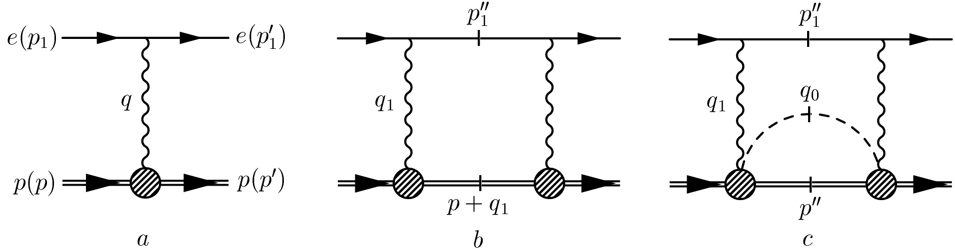
Figure 1: Polarized electron-proton elastic scattering: $a$ - Born approximation, $b$, $c$ - imaginary part of two photon exchange amplitude ($b$ - elastic intermediate state, $c$ - inelastic intermediate state).

The amplitude of elastic electron-proton-scattering, Eq. (1), taking into account only exchanged virtual photons, can be written as Bethe :

$$M(s,t)=e^{i\phi(t)}M_{1}(s,t),\quad\phi(t)=\frac{\alpha}{\pi}c\ln\left(\frac{-t}{\lambda^{2}}\right),$$ (3)

where $\lambda$ is a fictitious photon mass and $M_{1}$ is finite at the limit $\lambda\to 0$, $c$ is a real constant, depending on FFs and it is not calculated here.

In the language of Feynman diagrams, the phase factor $e^{i\phi}$ can be associated with single hadron intermediate hadronic states, whereas $M_{1}$ corresponds to inelastic intermediate hadronic states such as production of neutral pions.

The specific structure of the amplitude, Eq. 3, suggests a unique way to calculate TBSA, eliminating infrared divergences. The asymmetry indeed arises from the interference of the Born amplitude with the imaginary part of the two (or more) photon exchange amplitude in the lowest order of perturbation theory. The usual mechanism of infrared (IR) singularities cancellation (taking into account real soft photon emission) does not work here, since the amplitude of soft photon emission is real.

The interference of the Born amplitude with the two photon exchange amplitude where the intermediate state is a proton, leads to a result which can be expressed in the form $A\phi(t)+B$. Keeping in mind the general form of this scattering amplitude, Eq. 3, in order to eliminate the terms containing the phase $\phi(t)$, a regularization procedure, called IR regularization, has to be applied. It consists in dropping terms which contain $\ln(\lambda/m^{2})$. This is justified by the cancellation of infrared divergent terms when calculating the matrix element squared (3).

The general form for the contribution to the differential cross section for the case of transversally polarized incident electron is related to the factor

$$m(pp_{1}p^{\prime}_{1}a)=m\varepsilon_{\alpha\beta\gamma\delta}p^{\alpha}p_{1}^{\beta}p^{{}^{\prime}\gamma}_{1}a^{\delta}\simeq mMEE^{\prime}\sin\theta|a_{\perp}|,$$ (4)

where $m$, $M$, $E$, $E^{\prime}=E/\left[1+\frac{E}{M}(1-\cos\theta)\right]$ are the mass of electron, the mass of the proton, the energies of the initial and final electron, respectively, $\theta$ is the final electron scattering angle in the laboratory frame, and $a_{\perp}$ is the degree of transverse polarization of the incident electron.

The asymmetry is due to the interference of the Born amplitude with the $s$-channel imaginary part of two-photon exchange amplitude.

II.1 Elastic contribution

The elastic contribution to the asymmetry can be written as:

$$A_{el}=\frac{2\sum_{spin}M_{b}M^{*}_{el}}{\sum_{spin}|M_{b}|^{2}|a_{\bot}|},$$ (5)

with

$$\sum_{spin}|M_{b}|^{2} = \left(\frac{4\pi\alpha}{t}\right)^{2}8(s^{2}+u^{2}+2M^{2}t)F^{2}(t),$$

$$2\sum_{spin}M_{b}M^{*}_{el} = \frac{2^{5}\pi\alpha^{3}}{t}F(t)\frac{s}{s+M^{2}}\int S_{e}S_{el}\frac{dO^{\prime\prime}}{q^{2}_{1}q^{2}_{2}}F(t_{1})F(t_{2}),$$ (6)

where $q_{1,2}^{2}=-2\epsilon^{2}(1-c_{1,2})$ and $\epsilon=s/(2\sqrt{s+M^{2}})$ in the elastic case. The integration is performed in the center of mass system (CMS) of the initial particles, and $\epsilon$ is the energy of the electron in this reference frame. The proton vertex is described by such model for the Pauli and Dirac FFs: $F_{1}(t)=F(t)=(1+Q^{2}/Q_{0}^{2})^{-2}$ follows a dipole distribution with $Q_{0}^{2}=0.71$ GeV² and $F_{2}(t)=0$. This is a good approximation at very large or very small $t$ values. In our case, it is a simple prescription, which allows to factorize the terms containing FFs. The traces $S_{e}$ and $S_{el}$ have the form

$$S_{e} = \frac{1}{4}Tr(\hat{p}^{\prime}_{1}+m)\gamma_{\mu}(\hat{p}^{\prime\prime}_{1}+m)\gamma_{\nu}(\hat{p}_{1}+m)\gamma_{5}\hat{a}\gamma_{\lambda},$$ (7)

$$S_{el} = \frac{1}{4}Tr(\hat{p}^{\prime}+M)\gamma_{\mu}(\hat{p}+\hat{q}_{1}+M)\gamma_{\nu}(\hat{p}+M)\gamma_{\lambda}.$$ (8)

After performing the angular integration (see Appendix B) we obtain:

$$A_{el} = \frac{-st\alpha mMEE^{\prime}\sin\theta}{4(s+M^{2})(s^{2}+u^{2}+2M^{2}t)F(t)}Q_{el},$$ (9)

$$Q_{el} = -12a_{g}+(4s+6t)a_{1s}+2(s+t)a_{11}+[8M^{2}-2(2s+t)]a_{v}-4M^{2}I,$$ (10)

where the integrals $I$, $a_{v}$, $a_{11}$, $a_{1s}$, $a_{g}$ are given in the Appendix A (see Eq. (20)).

II.2 Inelastic contribution

The contribution of the inelastic channel can be written as:

$$A_{inel} = \frac{\alpha\cdot t}{64\pi^{2}}g^{2}\displaystyle\frac{|F(t)|^{-1}}{s^{2}+u^{2}+2M^{2}t}\int\frac{\epsilon^{\prime\prime}_{1}d\epsilon^{\prime\prime}_{1}}{q^{2}_{1}q^{2}_{2}}S_{e}S_{inel}\frac{dO_{\pi}dO^{\prime\prime}_{1}(s^{2}-2\sqrt{s+m^{2}}\epsilon^{\prime\prime}_{1})}{\pi^{2}[\sqrt{s-M^{2}}-\epsilon^{\prime\prime}_{1}(1-c_{\pi})]^{2}},$$

$$c_{\pi}=\cos\vec{p}_{1}{\!{}^{\prime}}\vec{q}_{0},\qquad m_{e}<\epsilon^{\prime\prime}_{1}<\frac{s}{2\sqrt{s+M^{2}}}\left(1-\frac{m_{\pi}M^{2}}{s\sqrt{s+M^{2}}}\right),$$

where the value of $g^{2}\leq 3$ can be extracted from the total photon-proton cross section $\sigma_{tot}^{\gamma p}\approx 0.1$ mb $>\alpha g^{2}/(4m_{\pi}^{2})$. The trace has the form:

$$S_{inel} = \frac{1}{4}Tr(\hat{p}^{\prime}+M)\left[\gamma_{5}\frac{\hat{p}^{\prime}-\hat{q}_{0}+M}{(p^{\prime}-q_{0})^{2}-M^{2}}\gamma_{\mu}+\gamma_{\mu}\frac{\hat{p}^{\prime\prime}+\hat{q}_{0}+M}{(p^{\prime\prime}+q_{0})^{2}-M^{2}}\gamma_{5}\right]\times$$ (12)

$$\times (\hat{p}^{\prime\prime}+M)\left[\gamma_{\nu}\frac{\hat{p}-\hat{q}_{0}+M}{(p-q_{0})^{2}-M^{2}}\gamma_{5}+\gamma_{5}\frac{\hat{p}^{\prime\prime}+\hat{q}_{0}+M}{(p^{\prime\prime}+q_{0})^{2}-M^{2}}\gamma_{\nu}\right](\hat{p}+M)\gamma_{\lambda},$$

where, in the inelastic case:

$$q^{2}_{1,2}=-\epsilon\epsilon^{\prime\prime}_{1}(1-\beta c_{1,2}),\quad 1-\beta^{2}=\left[\frac{m_{e}(\epsilon-\epsilon^{\prime\prime}_{1})}{\epsilon\epsilon^{\prime\prime}_{1}}\right]^{2}.$$ (13)

In the approximation of quadratic logarithms which is valid when $\epsilon^{\prime\prime}_{1}\ll M$ the resulting expression for asymmetry can be factorized (in CMS):

$$A_{inel}^{as}=-\frac{g^{2}\alpha mMEE^{\prime}s\sin\theta}{64\pi^{2}(s^{2}+u^{2}+2M^{2}t)(s+M^{2})F(t)}RP,$$ (14)

where $R$ is the contribution of the nucleon-pion block:

$$R = \eta-\frac{-2M^{2}+s+2t}{s}\delta+\left(\frac{2M^{2}}{s}-1\right)\gamma+2I_{L}+\left(4M^{2}-t\right)\alpha_{v}+$$ (15)

$$+2\left(2M^{2}+s\right)\beta_{v}+\frac{s\left(4\tau M^{2}+t\right)}{4M^{2}(\tau+1)}I_{1}+\frac{1}{s}j,\qquad\tau=\frac{-t}{4M^{2}}.$$

The coefficients $\eta$, $\delta$, $\gamma$, $I_{L}$, $\alpha_{v}$, $\beta_{v}$, $I_{1}$, $j$ are given in Appendix B, see Eq. (22), and the term $P$ is the contribution of the $2\gamma$-intermediate electron block of amplitude:

$$\int\frac{dO^{\prime\prime}\epsilon_{1}^{\prime\prime}d\epsilon_{1}^{\prime\prime}}{\pi q_{1}^{2}q_{2}^{2}}=-\frac{1}{t}\left[\ln\frac{-t}{m_{e}^{2}}\ln\frac{\epsilon^{2}}{m_{e}^{2}}-\frac{1}{2}\ln^{2}\frac{\epsilon^{2}}{m_{e}^{2}}+\frac{2\pi^{2}}{3}\right]=-\frac{1}{t}P.$$ (16)

III Results

Numerical results are presented in Tables 1 and 2 for different values of the outgoing electron scattering angle and of the energy of the initial electron.

The ratio $A_{el}/A^{as}_{inel}$ is given in Table 1 (see Eqs. (9,14). The elastic contribution is not negligible, representing more than 30 % of the inelastic one, for most of the kinematical region. At small energy and angle it even exceeds the inelastic contribution. The reason is that, at small energies, inelastic channels are suppressed in vicinity of the pion pair production threshold.

The total asymmetry $A=A_{el}+A^{as}_{inel}$ (in units ppm) is given in 2. It increases when the energy increases, around $\theta=90^{0}$ where it can be as large as 10⁴.

The suppression in the vicinity of $\theta=0$ or $\pi$, is driven by the sine term.

In order to compare the calculation with experimental data, different kinematical conditions should be considered, at low $Q^{2}$. The experimental values or Ref. Ma05 are well reproduced by the present calculation, taking the following values for the cosine of electron scattering angle: $a=0.64$ and for the pion coupling constant: $g^{2}=1.5$.

IV Conclusion

We calculated the contribution to the electron beam asymmetry in elastic $ep$ scattering, which arises from the two photon exchange amplitude in case of non excited hadron intermediate state. The present calculation shows that that the elastic contribution can not be neglected, and that it can be expressed in terms of hadron FFs.

The present results contradict previous statements of a specific suppression of this kind of contribution Mer ; Ruj ; Pasq ; AAM , the reason being that this source was not properly considered. The elastic intermediate state amplitude suffers from infrared divergences (see Eqs. (1), (3)). This fact was overlooked in the previous literature.

Inelastic hadronic intermediate states are enhanced in comparison with the elastic state considered above, and can be expressed in terms of double virtual Compton scattering (DVCS) amplitude Gorch contrary to statement AAM , where it was expressed in terms of photoproduction cross section.

Double logarithmic enhancement (DL) of inelastic channel takes place at higher orders of the QED coupling constant, what can lead to Sudakov form-factor suppresion type. Rigorous investigation of higher orders of QED contributions will be subject of further investigations.

It must be noted that the results are sensitive to the behavior of nucleon FFs, but do not chage the qualitatively results of the paper. The dipole like decreasing with the momentum transfer squared plays a crucial role and results in a general enhancement of elastic and inelastic channels contributions.

The choice of FFs taken in the present work, allows a simplified calculation. This approach is realistic at small $Q^{2}$ and at $Q^{2}\gg 1$ GeV² due to the suppression of the $F_{2}$ form factor. At small $Q^{2}$, the accuracy of our calculation, due to this approximation is of the order of $\tau$.

Another approximation, which affects the precision of the present results, is related to the fact that single-logarithmic terms of the form $\ln(-t/m^{2})$ as well as terms of the order $(m_{\pi}/M)^{2}$ were omitted.

Overall, the precision of the present results due to these approximations can be estimated at the level of 10 %.

V Acknowledgments

One of us (VB) is grateful to the grant MK-2952.2006.2. E.A.K. acknowledges the hospitality of DAPNIA/SPhN, Saclay, where part of this work was done.

$E$, GeV	$\theta=30^{0}$	$\theta=60^{0}$	$\theta=90^{0}$	$\theta=120^{0}$	$\theta=150^{0}$
1.0	-1.377	0.138	0.292	0.331	0.340
1.5	-0.252	0.323	0.379	0.392	0.392
2.0	0.123	0.377	0.389	0.394	0.401
2.5	0.261	0.375	0.378	0.381	0.377
3.0	0.327	0.358	0.363	0.359	0.354
3.5	0.349	0.361	0.339	0.338	0.338
4.0	0.348	0.335	0.327	0.314	0.316

Table 1: Ratio of elastic over inelastic terms $A_{el}/A_{inel}^{as}$.

$E$, GeV	$\theta=30^{0}$	$\theta=60^{0}$	$\theta=90^{0}$	$\theta=120^{0}$	$\theta=150^{0}$
1.00	0.76	-11.70	-28.27	-34.39	-23.037
1.50	-2.03	-22.13	-43.24	-43.96	-26.26
2.00	-4.47	-35.28	-58.57	-53.37	-29.87
2.50	-7.42	-50.05	-73.77	-62.71	-33.39
3.00	-11.119	-66.95	-88.68	-71.13	-37.69
3.50	-15.73	-85.08	-104.42	-79.98	-41.58
4.00	-21.58	-103.16	-119.07	-88.17	-45.32

Table 2: Total asymmetry $A=A_{el}+A^{as}_{inel}$ in units of ppm.

Appendix A Elastic contribution (method of integration)

The biaxial reference frame is used to parametrize the phase volume $dO^{\prime\prime}$ with fixed directions of initial ($\vec{p_{1}}$) and scattered ($\vec{p_{1}}{\,\!{}^{\prime}}$) electrons.

The angular phase space volume of the intermediate real electron is parametrized as

$$\int dO^{\prime\prime}=2\int\limits_{-1}^{1}dc_{1}\int\limits_{c_{-}}^{c_{+}}\frac{dc_{2}}{\sqrt{D}},$$

where

$$D = 1-a^{2}-c_{1}^{2}-c_{2}^{2}+2c_{1}c_{2}a=(c_{2}-c_{-})(c_{+}-c_{2})>0,$$

$$c_{\pm} = ac_{1}\pm\sqrt{(1-c_{1}^{2})(1-a^{2})},$$

and $c_{1}=\cos\theta_{1}$, $c_{2}=\cos\theta_{2}$, $a=\cos\theta_{c}$, and $\theta_{1}=\widehat{\vec{p}_{1}\vec{p_{1}}{\,\!{}^{\prime\prime}}}$, $\theta_{2}=\widehat{\vec{p_{1}}{\!{}^{\prime}}\vec{p_{1}}{\!{}^{\prime\prime}}}$, and $\theta_{c}=\widehat{\vec{p}_{1}\vec{p_{1}}{\,\!{}^{\prime}}}$ (in CMS, where $\vec{p}_{1}+\vec{p}=0$). Using Euler substitution ($t^{2}=(c_{2}-c_{-})/(c_{+}-c_{2})$) the relevant integrals are EK :

$$\int^{c_{+}}_{c_{-}}\frac{dc_{2}}{\sqrt{D}}=\pi;\quad\int^{c_{+}}_{c_{-}}\frac{dc_{2}}{\sqrt{D}(1-\beta c_{2})}=\frac{\pi}{[(a-\beta c_{1})^{2}+(1-\beta^{2})(1-c^{2}_{1})]^{\frac{1}{2}}};$$

$$\int^{c_{+}}_{c_{-}}\frac{c_{2}dc_{2}}{\sqrt{D}}=\pi ac_{1};$$

$$\int\frac{d^{2}c}{\sqrt{D}(1-\beta_{1}c_{1})(1-\beta_{2}c_{2})}=\frac{\pi}{\sqrt{d}}\left[\ln\left(\frac{4}{1-\beta^{2}_{1}}\right)+\ln\left(\frac{4}{1-\beta^{2}_{2}}\right)+2\ln\frac{1-\beta_{1}\beta_{2}a+\sqrt{d}}{4}\right],$$

$$d=(1-\beta_{1}\beta_{2}a)^{2}-(1-\beta^{2}_{1})(1-\beta^{2}_{2}),$$

where $\beta_{1}$ and $\beta_{2}$ are real number and $0<\beta_{1,2}<1$ .

For the case of a proton in the intermediate state one can write the following kinematical relations in CMS:

$$\vec{p}_{1}+\vec{p}=\vec{p}_{1}{{}^{\prime\prime}}+\vec{p}{\,{}^{\prime\prime}}=\vec{p}_{1}{\,\!{}^{\prime}}+\vec{p}{\,{}^{\prime}}=0;$$

$$-\lambda^{2}+q^{2}_{1}=(p_{1}-p^{\prime\prime}_{1})^{2}=-\lambda^{2}-2p^{2}(1-c_{1})=-2\epsilon^{2}(1-\beta_{\lambda}c_{1});$$

$$q^{2}=t=-2\epsilon^{2}(1-a),$$ (17)

with

$$1-\beta^{2}_{\lambda}=\displaystyle\frac{\lambda^{2}}{p^{2}},p^{2}\approx\epsilon^{2}\approx\displaystyle\frac{s^{2}}{4(s+M^{2})}.$$

Then the following integrals can be calculated:

$$I_{0} = \int\frac{dO^{\prime\prime}}{\pi(q^{2}_{1}-\lambda^{2})(q^{2}_{2}-\lambda^{2})}=-\frac{2}{t\epsilon^{2}}\ln{\left(\frac{-t}{\lambda^{2}}\right)},$$ (18)

$$I_{1} = \frac{1}{\pi}\int\frac{dO^{\prime\prime}}{q_{1}^{2}-\lambda^{2}}=-\frac{1}{\epsilon^{2}}\left[\ln\left(\frac{-t}{\lambda^{2}}\right)+\ln\left(\frac{4\epsilon^{2}}{-t}\right)\right].$$

Including a realistic hadron form factor $F(t)$, with normalization $F(0)=1$, after applying the IR regularization procedure, one obtains:

$$IR\int\frac{dO^{\prime\prime}F(q^{2}_{1})F(q^{2}_{2})}{(q^{2}_{1}-\lambda^{2})(q^{2}_{2}-\lambda^{2})}\left\{1,p^{\prime\prime}_{1\mu},p^{\prime\prime}_{1\mu}p^{\prime\prime}_{1\nu}\right\}=$$

$$\qquad\left\{I,\quad a_{v}(p_{1}+p^{\prime}_{1})_{\mu},\quad a_{g}g_{\mu\nu}+a_{11}(p_{1\mu}p_{1\nu}+p^{\prime}_{1\mu}p^{\prime}_{1\nu})+a_{1s}(p_{1\mu}p^{\prime}_{1\nu}+p_{1\nu}p^{\prime}_{1\mu})\right\},$$ (19)

where the scalar coefficients introduced in Eq. (10) have the form:

$$I = \frac{1}{2\epsilon^{4}}\left\{\int\frac{d^{2}c}{\sqrt{D}\pi}\frac{F(q^{2}_{1})-1}{1-c_{1}}\frac{F(q^{2}_{2})-1}{1-c_{2}}+\right.$$

$$+\left.\int^{1}_{-1}\frac{dc_{2}}{|c_{2}-a|}\left[\frac{F(q^{2}_{2})-1}{1-c_{2}}-\frac{F(t)-1}{1-a}\right]+\frac{F(t)-1}{1-a}L\right\},$$

$$a_{v} = \frac{-1}{t\epsilon^{2}\pi}\int\frac{d^{2}cF(q^{2}_{2})(F(q^{2}_{1})-1)}{\sqrt{D}(1-c_{1})}-\frac{1}{t\epsilon^{2}}\left[\int^{1}_{-1}\frac{dc_{2}[F(q^{2}_{2})-F(t)]}{|c_{2}-a|}+F(t)\cdot L\right],$$ (20)

$$a_{g} = \frac{1}{4}ta_{1s}=\frac{1}{t\pi}\int\frac{d^{2}c}{\sqrt{D}}F(q^{2}_{1})F(q^{2}_{2});\qquad L=\ln\left[\frac{s^{2}}{-t(s+M^{2})}\right]$$

$$a_{11} = -\frac{1}{\epsilon^{2}t^{2}}\left\{\int\frac{d^{2}cq^{2}_{2}F(q_{2}^{2})(F(q^{2}_{1})-1)}{\pi\sqrt{D}(1-c_{1})}\right.\left.+\int^{1}_{-1}\frac{dc_{2}}{|c_{2}-a|}(q^{2}_{2}F(q^{2}_{2})-tF(t))+tF(t)\cdot L\right\}.$$

It is easy to see that for any form of FFs (particularly for dipole ) all divergences are canceled and the final expressions are free from discontinuities. For our choice of FF we have:

$$\frac{F(q^{2}_{1,2})-1}{1-c_{1,2}}=\frac{-4\epsilon^{2}[Q^{2}_{0}+\epsilon^{2}(1-c_{1,2})]}{[Q^{2}_{0}+2\epsilon^{2}(1-c_{1,2})]^{2}},\quad\frac{F(t)-1}{1-a}=\frac{-4\epsilon^{2}[Q^{2}_{0}+\epsilon^{2}(1-a)]}{[Q^{2}_{0}+2\epsilon^{2}(1-a)]^{2}}.$$ (21)

Let us recall that the following relation holds between $a$, the cosine of scattering electron angle in CMS, and the initial electron energy, $\epsilon$: $1-a={-t}/(2\epsilon^{2})$ , and that $q^{2}_{1,2}=-2\epsilon^{2}(1-c_{1,2})$.

Appendix B Inelastic contribution (useful integrals)

In the inelastic case, after calculating the traces, the Schouten identity is used to express the loop momenta in the numerator via the denominators (we neglect the terms $m_{\pi}^{2}/M^{2}\approx 0.02$ compared to those of order unity):

$$c = \left(p^{\prime}-q_{0}\right)^{2}-M^{2}=-2p^{\prime}q_{0},$$

$$b = \left(p-q_{0}\right)^{2}-M^{2}=-2pq_{0},$$

$$d = \left(p^{\prime\prime}+q_{0}\right)^{2}-M^{2}=2p^{\prime\prime}q_{0}.$$

Finally, one can write the inelastic contribution in terms of the following integrals, Eq. (15):

$$\int d\omega\displaystyle\frac{1}{b} = \int d\omega\displaystyle\frac{1}{c}=I_{1}=-\frac{1}{4\epsilon^{2}}L,\qquad L=\ln\displaystyle\frac{s+M^{2}}{M^{2}},$$

$$\int d\omega\displaystyle\frac{b}{c} = \int d\omega\displaystyle\frac{c}{b}=\displaystyle\frac{1-a}{2\tilde{\beta}}L+a=I_{L},$$

$$\int d\omega\displaystyle\frac{b^{2}}{c} = -2\epsilon^{2}\beta\left\{\frac{1}{\tilde{\beta}}\left[\left(1-a\right)^{2}-\displaystyle\frac{1}{2}\left(1-\tilde{\beta}^{2}\right)\left(1-a^{2}\right)\right]L+2a-\frac{3}{2}a^{2}\right\}=i,$$

$$\int d\omega b = \int d\omega c=-2\epsilon^{2}\tilde{\beta}=j,\qquad\tilde{\beta}=\displaystyle\frac{s}{s+2M^{2}},$$

$$\int d\omega\displaystyle\frac{c}{b}q_{0}^{\mu} = (\gamma p+\delta p^{\prime})^{\mu},\qquad\gamma=\displaystyle\frac{1}{-16M^{4}\tau(1+\tau)}\left[(2M^{2}-t)i-2M^{2}j\right],$$ (22)

$$\int d\omega\displaystyle\frac{b}{c}q_{0}^{\mu} = (\gamma p^{\prime}+\delta p)^{\mu},\qquad\delta=\displaystyle\frac{1}{-16M^{4}\tau(1+\tau)}\left[(2M^{2}-t)j-2M^{2}i\right],$$

$$\int d\omega\displaystyle\frac{1}{c}q_{0}^{\mu} = (\alpha_{v}p+\beta_{v}Q)^{\mu},\qquad\alpha_{v}=\displaystyle\frac{1}{s^{2}}\left[2Q^{2}-s(M^{2}+Q^{2})I_{1}\right],$$

$$\int d\omega\displaystyle\frac{1}{b}q_{0}^{\mu} = (\alpha_{v}p^{\prime}+\beta_{v}Q)^{\mu},\qquad\beta_{v}=-\displaystyle\frac{1}{s^{2}}\left[M^{2}+Q^{2}+2M^{2}sI_{1}\right],$$

$$\int d\omega q_{0}^{\mu} = \eta Q^{\mu},\qquad\eta=\displaystyle\frac{s}{2Q^{2}},\qquad Q=p+p_{1},\qquad Q^{2}=M^{2}+s,$$

where the following notation holds for the phase volume element:

$$\frac{d^{3}q_{0}d^{3}p^{\prime\prime}}{2\epsilon_{0}2\epsilon^{\prime\prime}}\delta^{4}(Q-p^{\prime\prime}-q_{0})=\frac{s\pi}{2(s+M^{2})}d\omega,\qquad d\omega=\frac{dO_{\pi}}{4\pi}.$$ (23)

References

• (1) A. I. Akhiezer and M. P. Rekalo, Sov. Phys. Dokl.  13 (1968) 572 [Dokl. Akad. Nauk Ser. Fiz.  180 (1968) 1081].
• (2) A. I. Akhiezer and M. P. Rekalo, Sov. J. Part. Nucl.  4 (1974) 277 [Fiz. Elem. Chast. Atom. Yadra 4 (1973) 662].
• (3) M. K. Jones et al., Phys. Rev. Lett. 84 (2000) 1398; O. Gayou et al., Phys. Rev. Lett. 88 (2002) 092301; V. Punjabi et al., Phys. Rev. C 71 (2005) 055202, [Erratum-ibid. C 71 (2005) 069902].
• (4) P. A. M. Guichon and M. Vanderhaeghen, Phys. Rev. Lett.  91, 142303 (2003); Y. C. Chen, A. Afanasev, S. J. Brodsky, C. E. Carlson and M. Vanderhaeghen, Phys. Rev. Lett.  93, 122301 (2004).
• (5) J. Gunion and L. Stodolsky, Phys. Rev. Lett. 30, 345 (1973);
V. Franco, Phys. Rev. D 8, 826 (1973);
V. N. Boitsov, L.A. Kondratyuk and V.B. Kopeliovich, Sov. J. Nucl. Phys. 16, 237 (1973);
F. M. Lev, Sov. J. Nucl. Phys. 21, 45 (1973).
• (6) M. P. Rekalo, E. Tomasi-Gustafsson and D. Prout, Phys. Rev. C60, 042202 (1999).
• (7) E. Tomasi-Gustafsson and G. I. Gakh, Phys. Rev. C 72, 015209 (2005).
• (8) D. Borisyuk and A. Kobushkin, arXiv:nucl-th/0606030.
• (9) Yu. M. Bystritskiy, E. A. Kuraev and E. Tomasi-Gustafsson, arXiv:hep-ph/0603132; E. Tomasi-Gustafsson, arXiv:nucl-th/0602007.
• (10) E.A. Kuraev, V.V. Bytev, Yu.M. Bystritsky and E. Tomasi-Gustafsson, Phys.Rev. D74, 013003 (2006).
• (11) S. P. Wells et al. [SAMPLE collaboration], Phys. Rev. C 63, 064001 (2001).
• (12) F. E. Maas et al., Phys. Rev. Lett.  94, 082001 (2005).
• (13) A. V. Afanasev and N. P. Merenkov, Phys. Rev. D 70, 073002 (2004). P. G. Blunden, W. Melnitchouk and J. A. Tjon, Phys. Rev. Lett.  91, 142304 (2003);
• (14) B. Pasquini, M. Vanderhaeghen, hep-ph/0405303
• (15) M. Gorchtein, Phys. Rev. C 73, 035213 (2006).
• (16) A. De Rujula, J. M. Kaplan and E. De Rafael, Nucl. Phys. B 35, 365 (1971), Nucl. Phys. B 53, 545 (1973); F. Guerin, C. A. Picketty, Nuovo Cim. 32, 971 (1964); J. Arafune and Y. Shimizu, Phys. Rev. D 1, 3094 (1970); U. Guenther and R. Rodenberg, Nuovo Cim. A 2, 25 (1971); T. V. Kukhto, S. N. Panov, E. A. Kuraev and A. A. Sazonov, JINR-E2-92-556.
• (17) A. V. Afanasev and C. E. Carlson, Phys. Rev. Lett.  94, 212301 (2005).
• (18) H.A.Bethe, Annals of Phys. 3, 190 (1958); V. G. Gorshkov, E. A. Kuraev, L. N. Lipatov and M. M. Nesterov, Zh. Eksp. Teor. Fiz.  60, 1211 (1971).
• (19) E. A. Kuraev, Preprint INP 80-155, Novosibirsk (1980).
• (20) A. Afanasev, I. Akushevich, N.P. Merenkov, arXiv: hep-ph/0208260
• (21) L. Lipatov, private communication.