Non-Abelian energy loss in cold nuclear matter

Abstract

We use a formal recurrence relation approach to multiple parton scattering to find the complete solution to the problem of medium-induced gluon emission from partons propagating in cold nuclear matter. The differential bremsstrahlung spectrum, where Landau-Pomeranchuk-Migdal destructive interference effects are fully accounted for, is calculated for three different cases: (1) a generalization of the incoherent Bertsch-Gunion solution for asymptotic on-shell jets, (2) initial-state energy loss of incoming jets that undergo hard scattering and (3) final-state energy loss of jets that emerge out of a hard scatter. Our analytic solutions are given as an infinite opacity series, which represents a cluster expansion of the sequential multiple scattering. These new solutions allow, for the first time, direct comparison between initial- and final-state energy loss in cold nuclei. We demonstrate that, contrary to the naive assumption, energy loss in cold nuclear matter can be large. Numerical results to first order in opacity show that, in the limit of large jet energies, initial- and final-state energy losses exhibit different path length dependences, linear versus quadratic, in contrast to earlier findings. In addition, in this asymptotic limit, initial-state energy loss is considerably larger than final-state energy loss. These new results have significant implications for heavy ion phenomenology in both p+A and A+A reactions.

I Introduction

Non-Abelian final-state medium-induced radiative energy loss in the quark-gluon plasma (QGP) is the best studied many-body perturbative QCD (pQDC) application for high energy nuclear collisions. Several theoretical approaches that address this question have been well documented in recent reviews Gyulassy:2003mc ; Kovner:2003zj ; Baier:2000mf ; Vitev:2004bh ; Majum:2006 . In contrast, initial-state energy loss in cold nuclear matter, pertinent to hard jet and particle production in proton-nucleus (p+A) and nucleus-nucleus (A+A) collisions, has not been studied so far.

Strong motivation for in-depth investigation of cold nuclear matter energy loss comes from the finding that at most $1/2$ of the forward rapidity suppression in d+Au collisions measured at the Relativistic Heavy Ion Collider (RHIC) Arsene:2004ux ; Adams:2006uz can be accounted for by leading twist Guzey:2004zp or high twist Qiu:2004da shadowing calculations that take into account constraints from deep inelastic scattering (DIS) on nuclei. Moreover, at much lower center of mass energies at the Super Proton Synchrotron (SPS), a similar forward rapidity suppression is established and shown to not be compatible with shadowing calculations Vitev:2006bi .

Energy loss for asymptotic $t=\pm\infty$ on-shell jets that do not undergo hard scattering was discussed in Gunion:1981qs for nuclear matter of extent $L\sim r_{0}=1.2$ fm. It has been argued that the inclusion of the Landau-Pomeranchuk-Migdal (LPM) destructive interference effect Landau:1953 ; Migdal:1956tc for this regime, in the approximation of infinitely large number of soft scatterings, leads to negligible $\Delta E_{\rm rad}$, $1/3$ of the magnitude of final-state energy loss Baier:2000mf . Final-state energy loss in cold nuclei  Gyulassy:2003mc was found to have the same qualitative behavior as final-state energy loss in the QGP, though much smaller in magnitude and with possible relevance to suppressed hadron production in semi-inclusive DIS. None of these regimes can yield significant and phenomenologically relevant contribution to cold nuclear matter attenuation at collider energies.

Thus, the primary purpose of this manuscript is to derive and properly compare the Bertsch-Gunion, initial- and final-state energy loss in cold nuclei. The dominant contribution to $\Delta E_{\rm rad}$ can then be used in heavy ion QCD phenomenology prep . The secondary goal of this paper is to clarify the principle difference between radiative and collisional Mustafa:2004dr ; Adil:2006ei energy loss in cold/hot nuclear matter. Recent studies have made comparisons between $\Delta E_{\rm rad}$ and $\Delta E_{\rm col}$, emphasizing a deep LPM cancellation regime, which is not representative of the process of radiative energy loss. In addition, different and often incompatible formalisms are used in such comparisons.

We start by recalling the energy loss results for electrodynamics (QED) jackson . Consider medium of atomic density $\rho=N/V$. Each atom has $Z$ electrons of electric charge $e$ and mass $m$. An incident particle with electric charge $ze$ and mass $M$, $E=\gamma M$, $p=\beta\gamma M$, undergoes multiple Coulomb scattering in such a medium. Its collisional energy loss per unit length, including momentum transfers down to the mean excitation energy of the electrons $\langle\omega\rangle$, is given by:

$$\frac{d\Delta E_{coll}}{dx}\approx 64\pi^{3}\alpha_{em}^{2}z^{2}Z\rho\frac{1}{\beta^{2}m}\ln B_{q}\;.$$ (1)

In Eq. (1) $B_{q}=2\gamma^{2}\beta^{2}m/\langle\omega\rangle$ and in the high energy limit, $\ln B_{q}\gg\beta^{2}$, we have neglected a small correction to the large logarithm related to the relativistic electron spin. The physics behind collisional energy loss is the energy, $\Delta E_{\rm col}(Q^{2})$, transfered to the medium by the incident fast particle. Thus, one expects little dependence on the mass of the the incident particle, $M$, but strong dependence on the mass of the target scatterers, $m$. It is evident from Eq. (1) that collisional energy loss grows at most logarithmically with the energy of the incident particle, $E$, and linearly with the size of the medium, $L$.

On the other hand, the radiative energy loss per unit length is given by jackson :

$$\frac{d\Delta E_{rad}}{dx}\approx\frac{1024}{3}\pi^{3}\alpha_{em}^{3}z^{4}Z^{2}\rho\frac{1}{M^{2}}E\ln(\gamma\lambda)\;,$$ (2)

where $\lambda=\lambda(M,\gamma,\omega_{s})$ may also depend on the screening of the target electric charge via the characteristic frequency $\omega_{s}$. Radiative energy loss arises from the acceleration of the incident particle, which allows for emission of real photons. Thus, one expects that there will be significant dependence on the particle mass, $M$. Emitted photons naturally carry a fraction of the incident particle energy, implying that radiative energy loss is proportional to $E$ or, equivalently, $\gamma$. Both features are easily seen in Eq. (2) and $\Delta E_{\rm rad}$ grows linearly with $L$.

By comparing Eqs. (1) and (2) one observes that in the high energy regime $\Delta E_{\rm rad}\gg\Delta E_{\rm col}$. Thus, for ultra-relativistic particles radiative energy loss is the dominant mechanism of momentum attrition. As we will show below, the same energy dependence of $\Delta E_{\rm rad}$ is characteristic of QCD energy loss. It is only in the deep LPM regime for final-state energy loss that the energy dependence of $\Delta E_{\rm rad}$ is reduced to logarithmic. Since this is a very specific case, care should be taken to evaluate collisional energy loss in the same model of momentum transfers with the medium to the same power in the expansion in $1/p^{+}$.

This paper is organized as follows: in Section II we review the recursive approach to multiple parton scattering in both cold and hot nuclear matter, formulated in Gyulassy:2000er ; Gyulassy:2000fs . We use final-state energy loss as an example. Next, we derive to all orders in opacity the two new solutions for the radiative non-Abelian energy loss of incoming partons that may or may not undergo hard scattering that produces high-$p_{T}$ or high-$E_{T}$ particles or jets. Section III contains a detailed numerical study to first order in opacity of the three different energy loss regimes. We identify initial-state energy loss as the dominant cold nuclear matter $\Delta E_{\rm rad}$ contribution, relevant to p+A and A+A collider phenomenology. A summary and discussion of our results is given in Section IV. Appendixes contain useful kinematic simplifications, which allow for the derivation of the all-orders in opacity solutions given here. Explicit brute force calculations to second order in opacity of the new Bertsch-Gunion and initial-state $\Delta E_{\rm rad}$ are also shown for the purpose of validating the general results.

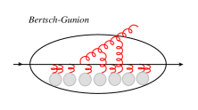
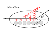
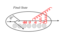
Figure 1: (Color online) Three distinct cases of medium-induced bremsstrahlung are illustrated: 1) Bertsch-Gunion case of $t=-\infty,t=+\infty$ on-shell jets; 2) initial-state energy loss in the nucleus followed by a large $Q^{2}$ process, resulting in the production of high-$p_{T}$ or high-$E_{T}$ particles and jets; 3) final-state energy loss in the nucleus, after a hard scatter.

II Recursive method for opacity expansion

For radiative processes in QCD, including medium-induced bremsstrahlung, it is important to keep track of the evolution of the gluon transverse momentum ${\bf k}$ in a plane perpendicular to the direction of jet propagation Gunion:1981qs . Such a ${\bf k}$ may arise from single hard or multiple soft scattering. The acceleration of the color charges in the 2D transverse plane generates color currents whose detailed interference pattern determines the strength of the non-Abelian Landau-Pomeranchuk-Migdal Landau:1953 ; Migdal:1956tc effect. Let us denote by:

$${\bf H} = {{\bf k}\over{\bf k}^{2}}\;,\qquad\qquad$$ (3)

$${\bf C}_{(i_{1}\cdots i_{m})} = {{\bf k}-{\bf q}_{i_{1}}-\cdots-{\bf q}_{i_{m}}\over({\bf k}-{\bf q}_{i_{1}}-\cdots-{\bf q}_{i_{m}})^{2}}\;,\qquad$$ (4)

$${\bf B}_{i_{1}} = {\bf H}-{\bf C}_{i_{1}}\;,\qquad$$ (5)

$${\bf B}_{(i_{1}\cdots i_{m})(j_{1}j_{2}\cdots i_{n})} = {\bf C}_{(i_{1}\cdots j_{m})}-{\bf C}_{(j_{1}j_{2}\cdots j_{n})}\;\;$$ (6)

the Hard, Cascade, and Bertsch-Gunion propagators in the transverse momentum space Gyulassy:2000er ; Gyulassy:2000fs . In Eqs. (3), (4), (5) and (6) ${\bf k}$ is the transverse momentum of the emitted gluon and ${\bf q}_{i}$ are the transverse momentum transfers from the medium to the jet+gluon system at positions $z_{i}$. Another important quantity, which enters the bremsstrahlung spectrum, is the formation time of the gluon, $\tau_{f}$, at the radiation vertex. When compared to the separation between the scattering centers $\Delta z_{j}=z_{j}-z_{j-1}$, which can fluctuate up to the size of the medium $L$, it determines the degree of coherence present in the multiple scattering process. We introduce the following notation Gyulassy:2000er ; Gyulassy:2000fs :

$$\tau_{0}^{-1}=\omega_{0} = \frac{{\bf k}^{2}}{k^{+}}\;,\qquad\qquad$$ (7)

$$\tau_{i_{1}}^{-1}=\omega_{i_{1}} = \frac{({\bf k}-{\bf q}_{i_{1}})^{2}}{k^{+}}\;,\qquad$$ (8)

$$\tau_{(i_{1}\cdots i_{m})}^{-1}=\omega_{(i_{1}\cdots i_{m})} = \frac{({\bf k}-{\bf q}_{i_{1}}-\cdots-{\bf q}_{i_{m}})^{2}}{k^{+}}\;.\qquad$$ (9)

In Eqs. (7), (8) and (9) $k^{+}$ is the large positive lightcone momentum of the bremsstrahlung gluon. We note that in calculating the amplitudes for the gluon emission, propagators of the type Eq. (3) - Eq. (6) come with a factor $-2ig_{s}\epsilon_{\perp}\cdot(\cdots)$ that we don’t write explicitly, see Appendix A. Similarly, at the level of squared amplitudes $\sum_{\rm polarizations}\epsilon_{\mu}^{\perp\,\star}\epsilon_{\nu}^{\perp}=-g^{\perp}_{\mu\nu}$. For physical quantities, this leaves us with the product of the 2D propagators in the amplitude and its conjugate.

II.1 Constructing the reaction operator

In the limit of high energy parton propagation in matter, multiple interactions are path ordered. The leading nuclear-size-enhanced contribution, $\propto L/\lambda$, to the modification of such partonic systems arises from two gluon exchanges with the strongly interacting constituents of the medium, as shown in Fig. 2. Unitarization of multiple scattering requires inclusion of three distinct cuts in the Feynman diagrams and is also illustrated. We note that $n>2$ gluon exchanges in the region of local color neutralization $1/\mu\ll\lambda$ will lead to higher order, $\propto\alpha^{n-2}$, corrections to the in-medium scattering, which are not nuclear size-enhanced. These are absorbed in the mean free path $\lambda$ for phenomenological applications. It is understood that all possible ways of attaching the momentum exchanges to the constituent partons of the propagating system should be considered, which increases the complexity of the calculation with the number of constituents. In the simplest case of single parton propagation, one can describe its transverse momentum diffusion due to the random walk in nuclear matter Gyulassy:2002yv . Recently, the dissociation of heavy mesons in the QGP has been calculated by applying this general approach to a $q\bar{q}$ system Adil:2006ra . Finally, the same classes of diagrams, shown in Fig. 2, were used to calculate direct photon and dilepton emission to first order in opacity Zhang:2006zd .

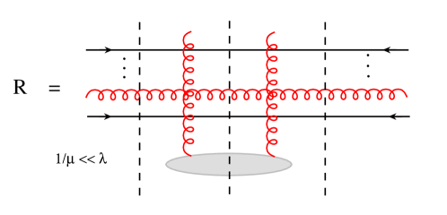
Figure 2: (Color online) Representation of the reaction operator for an arbitrary propagating system of partons. Three different cuts, corresponding to the relevant single-Born and double-Born interactions, are shown.

For the purpose of this paper, we are interested in a two-parton, jet+gluon, system propagation. The problem of radiative energy loss in QCD is more complicated than meson dissociation due to the multiple possibilities for the location of the gluon emission vertex in the many-body scattering. We first review Gyulassy:2000er the construction of the reaction operator, illustrated in Fig. 2. Let ${\cal A}_{i_{1}\cdots i_{n}}(x,{\bf k};c)$ be the amplitude when $n$ correlated interactions between the system and the medium may have already occurred. Here, $x=k^{+}/p^{+}$ and ${\bf k}$ are the kinematic variables and $c\equiv T_{c}$ is the color matrix associated with the radiative gluon. For each scattering center the system may: not interact; interact via a single-Born scattering; or interact via double-Born scattering. These correspond to the three possible cuts when an amplitude times its conjugate amplitude are considered. Therefore, the SU(3) color and kinematic modifications that arise from in-medium scattering at position $z_{m}$ are represented by the operators:

$$\hat{1}_{m}\;\;-\qquad{\rm Unit\;operator\;(no\;interaction)}\;,$$ (10)

$$\hat{D}_{m}\;\;-\qquad{\rm Direct\;operator\;(single-Born)}\;,$$ (11)

$$\hat{V}_{m}\;\;-\qquad{\rm Virtual\;operator\;(double-Born)}\;.\quad$$ (12)

Thus, starting with an initial condition $G_{0}(x,{\bf k};c)$, which can be the vacuum radiation associated with the hard scattering of the parton or the lack of such radiation for asymptotic on-shell jets Gyulassy:2000er ; Gyulassy:2000fs , we can construct the amplitude as follows:

$${\cal A}_{i_{1}\cdots i_{n}}(x,{\bf k},c) = \prod_{m=1}^{n}\left(\delta_{0,i_{m}}\hat{1}+\delta_{1,i_{m}}\hat{D}_{m}+\delta_{2,i_{m}}\hat{V}_{m}\right)$$ (13)

$$\times G_{0}(x,{\bf k};c)\;.$$

In Eq. (13) $\delta_{i,i_{m}}$ are the Kronecker symbols and the indexes $i_{m}$ keep track of which type of interaction, Eqs. (10), (11) and (12), has occurred. The operators are ordered from right to left as follows: $\hat{\cal{O}}_{i_{n}}\hat{\cal{O}}_{i_{n-1}}\cdots\hat{\cal{O}}_{i_{1}}$ for $i_{n}>i_{n-1}>\cdots>i_{1}$. The conjugate amplitude $\bar{\cal A}^{i_{1}\cdots i_{n}}(x,{\bf k};c)$ is then uniquely defined since no interaction is accompanied by a double-Born term, a single-Born interaction is accompanied by a single-Born term, and a double-Born interaction is accompanied by the unit term, see Fig. 2:

$$\bar{\cal A}^{i_{1}\cdots i_{n}}(x,{\bf k},c) = G_{0}^{\dagger}(x,{\bf k};c)\times$$ (14)

$$\prod_{m=1}^{n}\left(\delta_{0,i_{m}}\hat{V}_{m}^{\dagger}+\delta_{1,i_{m}}\hat{D}_{m}^{\dagger}+\delta_{2,i_{m}}\hat{1}^{\dagger}\right)\;.\qquad$$

In Eq. (14) the operators are ordered from left to right: $\hat{\cal{O}}_{i_{1}}^{\dagger}\cdots\hat{\cal{O}}_{i_{n-1}}^{\dagger}\hat{\cal{O}}_{i_{n}}^{\dagger}$ for $i_{n}>i_{n-1}>\cdots>i_{1}$ and act to the left.

The contribution to the cross section arising from $n$ correlated interactions can then be written as follows:

$$P_{n}(x,{\bf k}) = \bar{\cal A}^{i_{1}\cdots i_{n}}(c){\cal A}_{i_{1}\cdots i_{n}}(c)$$ (15)

$$\equiv {{\rm Tr}}\sum_{i_{1}=0}^{2}\cdots\sum_{i_{n}=0}^{2}{\cal A}^{\dagger}_{i_{1}\cdots i_{n}}(x,{\bf k};c){\cal A}_{i_{1}\cdots i_{n}}(x,{\bf k};c)\;\quad$$

$$= {{\rm Tr}}\sum_{i_{1}=0}^{2}\cdots\sum_{i_{n-1}=0}^{2}\bar{\cal A}^{i_{1}\cdots i_{n-1}}(x,{\bf k};c)\times$$

$$\left(\hat{D}_{n}^{\dagger}\hat{D}_{n}+\hat{V}_{n}+\hat{V}_{n}^{\dagger}\right){\cal A}_{i_{1}\cdots i_{n-1}}(x,{\bf k};c)\;.$$

From Eq. (15) we can identify the reaction operator,

$$\hat{R}\equiv\left(\hat{D}_{n}^{\dagger}\hat{D}_{n}+\hat{V}_{n}+\hat{V}_{n}^{\dagger}\right)\;,$$ (16)

as the basic input in this iterative approach to multiple scattering.

Clearly, to obtain the contribution from any number, $n$, of correlated interactions to the cross section (or the radiative gluon differential distribution) one has to:

1. Understand the structure of the direct and virtual operators, $\hat{D}_{n}$ and $\hat{V}_{n}$. The unit operator $\hat{1}$ is trivial.

2. Construct the reaction operator, Eq. (16).

3. Identify the relevant initial condition for the problem at hand, $\propto G_{0}^{\dagger}(x,{\bf k};c)G_{0}(x,{\bf k};c)$.

4. Solve the recurrence relation with this initial condition.

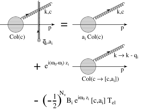
Figure 3: Diagrammatic representation of the sum of amplitudes generated by the direct single-Born scattering $\hat{D}_{i}{\cal A}$.

We first consider the action of the direct operator $\hat{D}_{n}$ at position $z_{n}$ on an amplitude with $n-1$ correlated scatterings. In this case, there is a single momentum transfer ${\bf q}_{i}$ in the amplitude and the same momentum transfer due to $\delta^{2}({\bf q}_{i}-{\bf q}_{i}^{\prime})$ in the conjugate amplitude Gyulassy:2000er , see Appendix A. The result of such action on ${\cal A}_{i_{1}\cdots i_{n-1}}$ can be represented as:

$$\hat{D}_{n}{\cal A}_{i_{1}\cdots i_{n-1}}(x,{\bf k};c)\equiv(a_{n}\hat{1}+\hat{S}_{n}+\hat{B}_{n}){\cal A}_{i_{1}\cdots i_{n-1}}(x,{\bf k};c)$$

$$=a_{n}{\cal A}_{i_{1}\cdots i_{n-1}}(x,{\bf k};c)$$

$$+e^{i(\omega_{0}-\omega_{n})z_{n}}{\cal A}_{i_{1}\cdots i_{n-1}}(x,{\bf k}-{\bf q}_{n};[c,a_{n}])$$

$$-\left(-{\textstyle\frac{1}{2}}\,\right)^{N_{v}({\cal A}_{i_{1}\cdots i_{n-1}})}{\bf B}_{n}\,e^{i\omega_{0}z_{n}}[c,a_{n}]T_{el}({\cal A}_{i_{1}\cdots i_{n-1}})\;\;.$$ (17)

The first term in Eq. (17) corresponds to a momentum exchange with the energetic jet. In the high energy limit terms of the type $p^{-}\sim(\sum_{i}{\bf q}_{i})^{2}/p^{+}$ are suppressed and we do not keep track of the transverse modification of the parent parton. Such interaction corresponds to an additional color factor $a_{n}$. The second term in Eq. (17) arises from the momentum transfer ${\bf q}_{n}$ to the radiative gluon, which cannot be neglected since the typical ${\bf k}\sim\sum_{i}{\bf q}_{i}$. If the gluon emerges with momentum ${\bf k}$ after the momentum transfer, in the amplitude ${\cal A}_{i_{1}\cdots i_{n-1}}$ it has momentum ${\bf k}-{\bf q}_{n}$. The interference phases $e^{i(\omega_{0}-\omega_{n})z_{n}}$ arise from the difference in the longitudinal momentum components before and after the the gluon interaction. Finally, if the gluon is represented by color matrix $c$, in the amplitude ${\cal A}_{i_{1}\cdots i_{n-1}}$ color is rotated as follows, $if^{ca_{n}d}d=[c,a_{n}]$, i.e. $c\rightarrow[c,a_{n}]$.

In addition to the above modifications to existing diagrammatic contributions for the amplitude with $n-1$ scattering centers, the acceleration at position $z_{n}$ acts as a source of a new color current, ${\bf B}_{n}$, with a phase factor $e^{i\omega_{0}z_{n}}$. Thus, the last term in Eq. (17) represents the diagrammatic contributions where the gluon is emitted immediately before or after the scattering center. In the former case, the gluon may also interact with this center. The parent parton has a cumulative color factor

$$T_{el}({\cal A}_{i_{1}\cdots i_{n-1}})\equiv(a_{n-1})^{i_{n-1}}\cdots(a_{1})^{i_{1}}\;,\qquad$$ (18)

$$T_{el}^{\dagger}(\bar{\cal A}^{i_{1}\cdots i_{n-1}})\equiv(a_{1})^{2-i_{1}}\cdots(a_{n-1})^{2-i_{n-1}}\;.$$ (19)

In the opacity expansion approach there is a unique relation between the color factors in the amplitude and its conjugate:

$$T^{\dagger}_{el}(\bar{\cal A}^{i_{1}\cdots i_{n-1}})T_{el}({\cal A}_{i_{1}\cdots i_{n-1}})=C_{R}^{n-1}\,{\bf 1}\;,$$ (20)

where $C_{R}$ is the quadratic Casimir in the fundamental or adjoint representations for quark or gluon parent partons, respectively. We denote by $N_{v}$ and $\bar{N}_{v}$ the number of double-Born interactions in the amplitude and its conjugate:

$$N_{v}=N_{v}({\cal A}_{i_{1}\cdots i_{n-1}})=\sum_{m=1}^{n-1}\delta_{2,i_{m}}\;,\qquad$$ (21)

$$\bar{N}_{v}=N_{v}(\bar{\cal A}^{i_{1}\cdots i_{n-1}})=\sum_{m=1}^{n-1}\delta_{0,i_{m}}\;,$$ (22)

and note that from a multinomial decomposition of zero we have:

$$\sum_{i_{1},\cdots,i_{m}}\left(-{\textstyle\frac{1}{2}}\right)^{N_{v}(\bar{\cal A}_{i_{1}\cdots i_{m}})}\left(-{\textstyle\frac{1}{2}}\right)^{N_{v}({\cal A}_{i_{1}\cdots i_{m}})}$$

$$\hskip 42.67912pt=\left(-{\textstyle\frac{1}{2}}-{\textstyle\frac{1}{2}}+1\right)^{m}=0\;.$$ (23)

The factor $(-1/2)^{N_{v}}$ arises from the symmetry in the two gluon legs at the same location $z_{m}$ and from the fact that when both momentum exchanges are in the amplitude or its conjugate we have $i^{2}=(-i)^{2}=-1$.

To summarize, for the medium-induced radiative problem in QCD, the single-Born or direct interaction can be represented as follows:

$$\hat{D}_{n}\equiv(a_{n}\hat{1}+\hat{S}_{n}+\hat{B}_{n})\;.$$ (24)

Here,

$$\hat{S}_{n}=if^{ca_{n}d}\times e^{i(\omega_{0}-\omega_{n})z_{n}}e^{i{\bf q}_{n}\cdot\hat{\bf b}}\;,$$ (25)

with $\hat{\bf b}\equiv i\stackrel{{\scriptstyle\longrightarrow}}{{{\nabla}_{\bf k}}}$ and $e^{i{\bf q}\cdot\hat{\bf b}}f({\bf k})=f({\bf k}-{\bf q})$. It is implicit that the color rotation $if^{ca_{n}d}d$, yielding $[c,a_{n}]$, is of the appropriate color matrix $d$ not shown explicitly in Eq. (25). The additional Bertsch-Gunion operator reads:

$$\hat{B}_{n} = -\left(-{\textstyle\frac{1}{2}}\right)^{N_{v}({\cal A}_{i_{1}\cdots i_{n-1}})}if^{ca_{n}d}d$$ (26)

$$\times\,{\bf B}_{n}\,e^{i\omega_{0}z_{n}}\;T_{el}({\cal A}_{i_{1}\cdots i_{n-1}})\;.$$

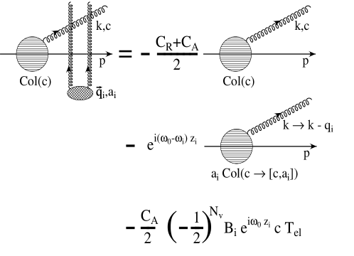
Figure 4: Diagrammatic representation of the sum of amplitudes generated by the virtual double-Born scattering $\hat{V}_{i}{\cal A}$.

Next, we consider the double-Born interaction of the jet at position $z_{n}$, as shown in Fig. 4. In this case there are two equal and opposite momentum transfers ${\bf q}_{i}$ in the amplitude (or the conjugate amplitude) due to $\delta^{2}({\bf q}_{i}+{\bf q}_{i}^{\prime})$ Gyulassy:2000er , see Appendix A. The modification of the amplitude ${\cal A}_{i_{1}\cdots i_{n-1}}(x,{\bf k};c)$ is found to be:

$$\hat{V}_{n}{\cal A}_{i_{1}\cdots i_{n-1}}(x,{\bf k};c)=-\frac{C_{R}+C_{A}}{2}{\cal A}_{i_{1}\cdots i_{n-1}}(x,{\bf k};c)$$

$$-e^{i(\omega_{0}-\omega_{n})z_{n}}a_{n}{\cal A}_{i_{1}\cdots i_{n-1}}(x,{\bf k}-{\bf q}_{n},[c,a_{n}])$$

$$-\left(-{\textstyle\frac{1}{2}}\,\right)^{N_{v}({\cal A}_{i_{1}\cdots i_{n-1}})}\frac{C_{A}}{2}\,{\bf B}_{n}\,e^{i\omega_{0}z_{n}}cT_{el}({\cal A}_{i_{1}\cdots i_{n-1}})\;.\qquad$$ (27)

The first term in Eq. (27) corresponds to the case when both momentum exchanges are with the parent parton or the radiative gluon. In this case there is no net momentum transfer, no additional phase factors arise and the two color matrices yield the quadratic Casimirs $C_{R}$ and $C_{A}$. The factor $(-1/2)$ was discussed above. The second term in Eq. (27) represents the situation where one of the gluon legs is attached to the jet and one to the bremsstrahlung gluon. Since there are two possible combinations $2\times(-1/2)=-1$ . The shift in the transverse momentum ${\bf k}\rightarrow{\bf k}-{\bf q}_{n}$, the phase factor $e^{i(\omega_{0}-\omega_{n})z_{n}}$ and the color rotation $if^{ca_{n}d}d$, i.e. $c\rightarrow[c,a_{n}]$, are all the same as in the second term in Eq. (17). The difference is that the interaction with the parent parton gives an additional color factor $a_{n}$. Finally, parts of the diagrams where a gluon is emitted immediately before or after the interaction point $z_{n}$ are combined in the last term in Eq. (27). This term is identical to the last term in Eq. (17), except for the color factor since we have carried out the simplification $a_{n}[c,a_{n}]=-(C_{A}/2)c$. The additional $(-1)$ arises from the last two gluon exchanges at $z_{n}$. In summary, the double-Born interaction at $z_{n}$ can be implemented by the following operator

$$\hat{V}_{n} = -{\textstyle\frac{1}{2}}(C_{A}+C_{R})\hat{1}-a_{n}\hat{S}_{n}-a_{n}\hat{B}_{n}$$ (28)

$$= -a_{n}\hat{D}_{n}-{\textstyle\frac{1}{2}}(C_{A}-C_{R})\;,$$

and is clearly not linearly independent of the single-Born term, Eq. (24).

Now, we can proceed and construct the reaction operator $\hat{R}_{n}$ to relate the $n^{\rm th}$ order in opacity gluon emission “probability” distribution $P_{n}(x,k)$ to the probability at $(n-1)^{\rm st}$ order. We express the reaction operator in Eq. (16) as follows:

$$\hat{R}_{n} = (\hat{D}_{n}-a_{n})^{\dagger}(\hat{D}_{n}-a_{n})-C_{A}\hat{1}$$ (29)

$$= (\hat{S}_{n}+\hat{B}_{n})^{\dagger}(\hat{S}_{n}+\hat{B}_{n})-C_{A}\hat{1}$$

$$= (\hat{S}_{n}^{\dagger}\hat{S}_{n}-C_{A}\hat{1})+\hat{B}_{n}^{\dagger}\hat{B}_{n}+2{\cal R}e\;\hat{S}_{n}^{\dagger}\hat{B}_{n}\;.\quad$$

Noting that $if^{ca_{n}d}(-i)f^{ca_{n}d^{\prime}}=C_{A}\delta_{d,d^{\prime}}$, we see that the first term in Eq. (29),

$$(\hat{S}_{n}^{\dagger}\hat{S}_{n}-C_{A}\hat{1}) = C_{A}(e^{-{\bf q}_{n}\stackrel{{\scriptstyle\leftarrow}}{{{\nabla}_{{\bf k}}}}}e^{-{\bf q}_{n}\stackrel{{\scriptstyle\rightarrow}}{{{\nabla}_{{\bf k}}}}}-\hat{1})\;,$$ (30)

gives a homogeneous contribution to the functional recurrence relation:

$$\bar{\cal A}^{i_{1}\cdots i_{n-1}}(x,{\bf k};c)(\hat{S}_{n}^{\dagger}\hat{S}_{n}-C_{A}){\cal A}_{i_{1}\cdots i_{n-1}}(x,{\bf k};c)$$

$$\qquad=C_{A}\left(P_{n-1}(x,{\bf k}-{\bf q}_{n})-P_{n-1}(x,{\bf k})\right)$$

$$\qquad=C_{A}\left(e^{i{\bf q}_{n}\cdot\hat{\bf b}}-1\right)P_{n-1}(x,{\bf k})\;.$$ (31)

The second term does not contribute beyond first order in opacity, $n=1$, since

$$\bar{\cal A}^{i_{1}\cdots i_{n-1}}(x,{\bf k};c)\hat{B}_{n}^{\dagger}\hat{B}_{n}{\cal A}_{i_{1}\cdots i_{n-1}}(x,{\bf k};c)=C_{A}\,|{\bf B}_{n}|^{2}$$

$$\quad\times\sum_{i_{1},\cdots,i_{n-1}}\left(-{\textstyle\frac{1}{2}}\right)^{\bar{N}_{v}(\bar{\cal A}^{i_{1}\cdots i_{n-1}})}\left(-{\textstyle\frac{1}{2}}\right)^{N_{v}({\cal A}_{i_{1}\cdots i_{n-1}})}$$

$$\quad\times\;T_{el}^{\dagger}(\bar{\cal A}^{i_{1}\cdots i_{n-1}})\,cc\,T_{el}({\cal A}_{i_{1}\cdots i_{n-1}})\equiv 0\;.\qquad$$ (32)

For this proof we used Eq. (20), and the identity (23). For $n=1$, however, the $C_{R}C_{A}|{\bf B}_{1}|^{2}$ contribution to $P_{n-1}(x,{\bf k})$ survives. Finally, the non-diagonal term in Eq. (29) reads:

$$2{\cal R}e\,\bar{\cal A}^{i_{1}\cdots i_{n-1}}(x,{\bf k};c)\hat{B}_{n}^{\dagger}\hat{S}_{n}{\cal A}_{i_{1}\cdots i_{n-1}}(x,{\bf k};c)$$

$$=-2C_{A}\,{\bf B}_{n}\cdot\left({\rm Re}\;e^{-i\omega_{n}z_{n}}e^{i{\bf q_{n}}\cdot\hat{\bf b}}{\bf I}_{n-1}\right)\;,$$ (33)

where we have used Eqs. (25) and (26). Writing explicitly the expression for ${\bf I}_{n-1}$ and representing the $(n-1)^{\rm th}$ step in this iteration via the $\hat{S}_{n-1}$ and $\hat{B}_{n-1}$ operators we obtain:

$${\bf I}_{n-1}=\sum_{i_{1}\cdots i_{n-1}}\left(-{\textstyle\frac{1}{2}}\right)^{N_{v}(\bar{\cal A}^{i_{1}\cdots i_{n-1}})}T_{el}^{\dagger}(\bar{\cal A}^{i_{1}\cdots i_{n-1}})$$

$$\hskip 42.67912pt\times c{\cal A}_{i_{1}\cdots i_{n-1}}(x,{\bf k};c)$$

$$=\sum_{i_{1}\cdots i_{n-2}}\left(-{\textstyle\frac{1}{2}}\right)^{N_{v}(\bar{\cal A}_{i_{1}\cdots i_{n-2}})}T_{el}^{\dagger}(\bar{\cal A}_{i_{1}\cdots i_{n-2}})$$

$$\times\,\left[C_{A}(e^{i(\omega_{0}-\omega_{n-1})z_{n-1}}e^{i{\bf q}_{n-1}\cdot\hat{\bf b}}-1)c+[a_{n-1},c]\hat{B}_{n-1}\right]$$

$$\times\,{\cal A}_{i_{1}\cdots i_{n-2}}(x,{\bf k};c)\;.$$ (34)

In Eq. (34) the term proportional to $\hat{B}_{n-1}{\cal A}_{i_{1}\cdots i_{n-2}}$ vanishes for $n>2$. The proof, up to an insignificant difference in color factors, is again based on the multinomial decomposition of zero, Eq. (23).

From Eqs. (30) and (33), the basic iteration step for the full solution of the problem of medium induced gluon radiation can be written as follows:

$$P_{n}(x,{\bf k}) = C_{A}\left(P_{n-1}(x,{\bf k}-{\bf q}_{n})-P_{n-1}(x,{\bf k})\right)$$ (35)

$$-2C_{A}\,{\bf B}_{n}\cdot\left({\cal R}e\;e^{-i\omega_{n}z_{n}}e^{i{\bf q_{n}}\cdot\hat{\bf b}}{\bf I}_{n-1}\right)$$

$$+\delta_{n,1}C_{A}C_{R}|{\bf B}_{1}|^{2}\;.$$

The inhomogeneous term in Eq. (35) is expressed as:

$${\bf I}_{n-1} = C_{A}\left(e^{i(\omega_{0}-\omega_{n-1})z_{n-1}}e^{i{\bf q}_{n-1}\cdot\hat{\bf b}}-1\right){\bf I}_{n-2}$$ (36)

$$-\delta_{n-1,1}C_{A}C_{R}{\bf B}_{1}e^{i\omega_{0}z_{1}}\,,$$

which is a direct consequence of Eq. (34).

We emphasize that each radiative problem yields a different solution, related to the boundary condition $G_{0}(x,{\bf k};c)$. For final-state radiation this initial condition is given by the bremsstrahlung associated with the hard scattering of incoming partons. This case has been considered in detail in Ref. Gyulassy:2000er as the first complete application of the GLV approach. Explicit solution to all orders in the correlation between the momentum transfers from the multiple scattering centers to the jet+gluon system, suitable for further analytic approximations or numerical simulations, has been found for the case of final-state radiation, the third case illustrated in Fig. 1. We emphasize that these are not correlations between the scattering centers of the target arising from the strong nuclear force. Subject to the coherence criterion, $\tau_{f}\geq\max(|z_{i}-z_{j}|,0\leq i,j\leq n)$ at $n^{\rm th}$ order in opacity, the momentum transfers are correlated in the sense that the bremsstrahlung from the hard collision (at position $z_{0}$) and the multiple soft interactions (at positions $z_{j}>z_{0}$) interfere to give a contribution to the medium-induced spectrum of gluons. For completeness, we quote the result here Gyulassy:2000er :

$$k^{+}\frac{dN^{g}(FS)}{dk^{+}d^{2}{\bf k}} = \frac{C_{R}\alpha_{s}}{\pi^{2}}\sum_{n=1}^{\infty}\left[\prod_{i=1}^{n}\int\frac{d\Delta z_{i}}{\lambda_{g}(z_{i})}\right]\left[\prod_{j=1}^{n}\int d^{2}{\bf q}_{j}\left(\frac{1}{\sigma_{el}(z_{j})}\frac{d\sigma_{el}(z_{j})}{d^{2}{\bf q}_{j}}-\delta^{2}({\bf q}_{j})\right)\right]$$ (37)

$$\times\;\left[-2\,{\bf C}_{(1,\cdots,n)}\cdot\sum_{m=1}^{n}{\bf B}_{(m+1,\cdots,n)(m,\cdots,n)}\left(\cos\left(\,\sum_{k=2}^{m}\omega_{(k,\cdots,n)}\Delta z_{k}\right)-\cos\left(\,\sum_{k=1}^{m}\omega_{(k,\cdots,n)}\Delta z_{k}\right)\right)\;\right]\;,\qquad$$

where $\sum_{2}^{1}\equiv 0$ and ${\bf B}_{(n+1,n)}\equiv{\bf B}_{n}$ is understood. In the case of final-state interactions, $z_{0}\approx 0$ is the point of the initial hard scatter and $z_{L}=L$ is the extent of the medium. The path ordering of the interaction points, $z_{L}>z_{j+1}>z_{j}>z_{0}$, leads to the constraint $\sum_{i=1}^{n}\Delta z_{i}\leq z_{L}$. One implementation of this condition would be $\Delta z_{i}\in[\,0,z_{L}-\sum_{j=1}^{i-1}\Delta z_{j}\,]$ and it is implicit in Eq. (37). If we write the 2D propagators and interference phases in Eq. (37) more explicitly, we have:

$$k^{+}\frac{dN^{g}(FS)}{dk^{+}d^{2}{\bf k}} = \frac{C_{R}\alpha_{s}}{\pi^{2}}\sum_{n=1}^{\infty}\left[\prod_{i=1}^{n}\int{d\Delta z_{i}}\;{\sigma_{el}(z_{i})\rho(z_{i})}\right]\left[\prod_{j=1}^{n}\int d^{2}{\bf q}_{j}\left(\frac{1}{\sigma_{el}(z_{j})}\frac{d\sigma_{el}(z_{j})}{d^{2}{\bf q}_{j}}-\delta^{2}({\bf q}_{j})\right)\right]$$ (38)

$$\times\;\left[-2\;\frac{{\bf k}-{\bf q}_{1}-\cdots-{\bf q}_{n}}{({\bf k}-{\bf q}_{1}-\cdots-{\bf q}_{n})^{2}}\cdot\sum_{m=1}^{n}\left(\frac{{\bf k}-{\bf q}_{m+1}-\cdots-{\bf q}_{n}}{({\bf k}-{\bf q}_{m+1}-\cdots-{\bf q}_{n})^{2}}-\frac{{\bf k}-{\bf q}_{m}-\cdots-{\bf q}_{n}}{({\bf k}-{\bf q}_{m}-\cdots-{\bf q}_{n})^{2}}\right)\right.$$

$$\left.\times\;\left(\cos\left(\sum_{k=2}^{m}\frac{({\bf k}-{\bf q}_{k}-\cdots-{\bf q}_{n})^{2}}{k^{+}}\Delta z_{j}\right)-\cos\left(\sum_{k=1}^{m}\frac{({\bf k}-{\bf q}_{k}-\cdots-{\bf q}_{n})^{2}}{k^{+}}\Delta z_{j}\right)\;\right)\;\right]\;.$$

Jet quenching in the QGP, the best known application of non-Abelian energy loss in heavy ion reactions, is based on such a solution. For details, see Gyulassy:2003mc .

II.2 Bertsch-Gunion radiation to all orders in opacity

The first new solution that we obtain is this paper is for the case of asymptotic on-shell jets, initially considered by Bertsch and Gunion Gunion:1981qs and illustrated as the first case in Fig. 1. Although it is not directly applicable to the physics situation of high-$p_{T}$ particle production due to the lack of hard scattering, it is a necessary step to fully solve the problem of initial-state energy loss. The absence of hard bremsstrahlung yields a simple initial condition:

$$G_{0}(x,{\bf k};c)=0\;.$$ (39)

The solution for the ${\bf I}_{n-1}$ part in the inhomogeneous term of Eq. (35) reads:

$${\bf I}_{0} = 0\;,$$ (40)

$${\bf I}_{1} = -C_{A}C_{R}{\bf B}_{1}e^{i\omega_{0}z_{1}}\;,$$ (41)

$${\bf I}_{n-1} = -C_{R}C_{A}^{n-1}\prod_{m=2}^{n-1}\left(e^{i(\omega_{0}-\omega_{m})z_{m}}e^{i{\bf q}_{m}\cdot\hat{\bf b}}-1\right)$$ (42)

$$\times\,{\bf B}_{1}e^{i\omega_{0}z_{1}}\;.$$

Consequently, the solution for $P_{n}(x,{\bf k})$ can be written in the form

$$P_{n}(x,{\bf k}) = C_{R}C_{A}^{n}\prod_{m=2}^{n}(e^{i{\bf q}_{m}\cdot\hat{\bf b}}-1)|{\bf B}_{1}|^{2}+2{\cal R}e\,C_{R}C_{A}^{n}\sum_{m=2}^{n}\left[\prod_{j=m+1}^{n}(e^{i{\bf q}_{j}\cdot\hat{\bf b}}-1)\right]\,{\bf B}_{m}e^{i{\bf q}_{m}\cdot\hat{\bf b}}e^{-i\omega_{0}z_{m}}$$ (43)

$$\times\;\prod_{j=2}^{m-1}(e^{i(\omega_{0}-\omega_{j})z_{j}}e^{i{\bf q}_{j}\cdot\hat{\bf b}}-1)\,{\bf B}_{1}e^{i\omega_{0}z_{1}}\;.$$

In Eq. (43) we recall that, for the special case of $n=1$, $\sum_{i=2}^{1}=0$ and $\prod_{i=2}^{1}=1$. It is easy to verify that our result is a solution of the master recurrence relation Eq. (35) by rewriting it in the form:

$$P_{n}(x,{\bf k}) = C_{A}(e^{i{\bf q}_{n}\cdot\hat{\bf b}}-1)\left[C_{R}C_{A}^{n-1}\prod_{m=2}^{n-1}(e^{i{\bf q}_{m}\cdot\hat{\bf b}}-1)|{\bf B}_{1}|^{2}+2{\cal R}e\,C_{R}C_{A}^{n-1}\sum_{m=2}^{n-1}\left[\prod_{j=m+1}^{n-1}(e^{i{\bf q}_{j}\cdot\hat{\bf b}}-1)\right]\,{\bf B}_{m}e^{i{\bf q}_{m}\cdot\hat{\bf b}}e^{-i\omega_{0}z_{m}}\right.$$ (44)

$$\left.\times\;\prod_{j=2}^{m-1}C_{A}(e^{i(\omega_{0}-\omega_{j})z_{j}}e^{i{\bf q}_{j}\cdot\hat{\bf b}}-1)\,{\bf B}_{1}e^{i\omega_{0}z_{1}}\right]\;+2{\cal R}e\,C_{R}C_{A}^{n}{\bf B}_{n}e^{i{\bf q}_{n}\cdot\hat{\bf b}}e^{-i\omega_{0}z_{n}}\prod_{j=2}^{n-1}C_{A}(e^{i(\omega_{0}-\omega_{j})z_{j}}e^{i{\bf q}_{j}\cdot\hat{\bf b}}-1)$$

$$\times\;{\bf B}_{1}e^{i\omega_{0}z_{1}}\;.$$

To obtain the contribution of $n$ correlated scatterings to medium-induced gluon production we have to average over the momentum transfers ${\bf q}_{n}$ in Eq. (43). Let $(1/\sigma_{el})d\sigma_{el}/d^{2}{\bf q}_{m}$ be the differential distribution of momentum transfers at position $z_{m}$. We note that the first term in Eq. (43) can be written as follows,

$$\left[\prod_{i=1}^{n}\int d^{2}{\bf q}_{i}\;\frac{1}{\sigma_{el}}\frac{d\sigma_{el}}{d^{2}{\bf q}_{i}}\right]\prod_{m=2}^{n}(e^{i{\bf q}_{m}\cdot\hat{\bf b}}-1)|{\bf B}_{1}|^{2}$$ (45)

$$= \left[\prod_{i=1}^{n}\int d^{2}{\bf q}_{i}\;\left(\frac{1}{\sigma_{el}}\frac{d\sigma_{el}}{d^{2}{\bf q}_{i}}-\delta^{2}({\bf q}_{i})\right)\right]\,$$

$$\times\,\prod_{m=2}^{n}e^{i{\bf q}_{m}\cdot\hat{\bf b}}\;|{\bf B}_{1}|^{2}\;.$$

In Eq. (45) we are able to carry out the simplification including the $n=1$ term since

$$\delta^{2}({\bf q}_{i})\,{\bf B}_{i}=0\;.$$ (46)

The inhomogeneous term in Eq. (43) can also be simplified. For the momentum transfers ${\bf q}_{m+1},\cdots,{\bf q}_{n}$ the result follows from Eq. (45). For the momentum transfers ${\bf q}_{2},\cdots,{\bf q}_{m-1}$ we use

$$\left[\prod_{i=2}^{m-1}\int d^{2}{\bf q}_{j}\;\frac{1}{\sigma_{el}}\frac{d\sigma_{el}}{d^{2}{\bf q}_{i}}\right]\prod_{j=2}^{m-1}\left(e^{i(\omega_{0}-\omega_{j})z_{j}}e^{i{\bf q}_{j}\cdot\hat{\bf b}}-1\right)$$ (47)

$$\times{\bf B}_{1}e^{i\omega_{0}z_{1}}$$

$$= \left[\prod_{i=2}^{m-1}\int d^{2}{\bf q}_{i}\;\left(\frac{1}{\sigma_{el}}\frac{d\sigma_{el}}{d^{2}{\bf q}_{i}}-\delta^{2}({\bf q}_{i})\right)\right]$$

$$\times\prod_{j=2}^{m-1}e^{i(\omega_{0}-\omega_{j})z_{j}}e^{i{\bf q}_{j}\cdot\hat{\bf b}}\;{\bf B}_{1}e^{i\omega_{0}z_{1}}\;.$$

We note that the terms $n=1$ and $n=m$ can also be included in the general representation, Eq. (47), due to Eq. (46). Thus, we write the contribution of the multiple scattering centers as follows:

$$\left[\prod_{i=1}^{n}\int d^{2}{\bf q}_{i}\;\frac{1}{\sigma_{el}}\frac{d\sigma_{el}}{d^{2}{\bf q}_{i}}\right]\;P_{n}(x,{\bf k})=C_{R}C_{A}^{n}\left[\prod_{i=1}^{n}\int d^{2}{\bf q}_{i}\;\left(\frac{1}{\sigma_{el}}\frac{d\sigma_{el}}{d^{2}{\bf q}_{i}}-\delta^{2}({\bf q}_{i})\right)\right]\;\left[\prod_{m=2}^{n}e^{i{\bf q}_{m}\cdot\hat{\bf b}}\;|{\bf B}_{1}|^{2}\right.$$

$$\qquad\qquad\qquad\left.+2{\cal R}e\,\sum_{m=2}^{n}\left[\prod_{j=m+1}^{n}e^{i{\bf q}_{j}\cdot\hat{\bf b}}\right]\,{\bf B}_{m}e^{i{\bf q}_{m}\cdot\hat{\bf b}}e^{-i\omega_{0}z_{m}}\;\prod_{j=2}^{m-1}e^{i(\omega_{0}-\omega_{j})z_{j}}e^{i{\bf q}_{j}\cdot\hat{\bf b}}\,{\bf B}_{1}e^{i\omega_{0}z_{1}}\right]\;.$$ (48)

We note again that in Eq. (48) the products of momentum shift operators or phases and momentum shift operators are applied sequentially from the left with each operator acting on the function resulting from the previous one.

The last step in writing the explicit solution is to carry out the action of the momentum shift operators in Eq. (48). The first homogeneous term can be easily simplified since

$$\prod_{m=2}^{n}e^{i{\bf q}_{m}\cdot\hat{\bf b}}\;|{\bf B}_{1}|^{2}=|{\bf B}_{(2\cdots n)(1\cdots n)}|^{2}\;.$$ (49)

The inhomogeneous term can also be simplified as follows:

$$\prod_{j=m+1}^{n}e^{i{\bf q}_{j}\cdot\hat{\bf b}}\,{\bf B}_{m}e^{i{\bf q}_{m}\cdot\hat{\bf b}}e^{-i\omega_{0}z_{m}}\;$$

$$\qquad\qquad\times\prod_{j=2}^{m-1}e^{i(\omega_{0}-\omega_{j})z_{j}}e^{i{\bf q}_{j}\cdot\hat{\bf b}}\,{\bf B}_{1}e^{i\omega_{0}z_{1}}$$

$$={\bf B}_{(m+1\cdots n)(m\cdots n)}e^{i\sum_{j=m}^{n}{\bf q}_{j}\cdot\hat{\bf b}}$$

$$\;\;\times\,e^{-i\sum_{j=2}^{m}\omega_{(j\cdots m-1)}(z_{j}-z_{j-1})}{\bf B}_{(2\cdots m-1)(1\cdots m-1)}\;.\quad$$

$$={\bf B}_{(m+1\cdots n)(m\cdots n)}\cdot{\bf B}_{(2\cdots n)(1\cdots n)}$$

$$\quad\times e^{-i\sum_{j=2}^{m}\omega_{(j\cdots m-1)}\Delta z_{j}}\;.$$ (50)

The overall normalization for the differential gluon distribution is set by the color factor, the strong coupling constant and a phase space factor that combine to produce the factor $C_{R}\alpha_{s}/\pi^{2}$. We note that $C_{R}$ signifies the color charge dependence of the gluon bremsstrahlung in the small energy loss limit $\Delta E_{\rm rad}/E\ll 1$. Similarly to the case of final state gluon bremsstrahlung, in the limit of small lightcone momentum fractions $x$ and small transverse momenta ${\bf k}$ the result is “color trivial”, retaining only the quadratic Casimirs in the adjoint representation. These enter the mean free path of the propagating jet+gluon system, indicating that only gluon rescattering is important, i.e. $\lambda_{g}(z_{i})$. Putting everything together we find:

$$k^{+}\frac{dN^{g}(BG)}{dk^{+}d^{2}{\bf k}} = \frac{C_{R}\alpha_{s}}{\pi^{2}}\left[\prod_{i=1}^{n}\int\frac{d\Delta z_{i}}{\lambda_{g}(z_{i})}\right]\left[\prod_{j=1}^{n}\int d^{2}{\bf q}_{j}\left(\frac{1}{\sigma_{el}(z_{j})}\frac{d\sigma_{el}(z_{j})}{d^{2}{\bf q}_{j}}-\delta^{2}({\bf q}_{j})\right)\right]$$ (51)

$$\times\;{\bf B}_{(2\cdots n)(1\cdots n)}\cdot\left[{\bf B}_{(2\cdots n)(1\cdots n)}+2\sum_{i=2}^{n}{\bf B}_{(i+1\cdots n)(i\cdots n)}\cos\left(\sum_{j=2}^{i}\omega_{(j\cdots n)}\Delta z_{j}\right)\right]\;.$$

A direct comparison of this general result to the brute force calculation up to second order in opacity can be found in Appendix B. The integration limits on the separation between the multiple scattering centers were discussed in the previous section. Since in this case there is no hard scattering, the maximum separation corresponds to the physical size of the medium. More explicitly, our result reads:

$$k^{+}\frac{dN^{g}(BG)}{dk^{+}d^{2}{\bf k}} = \frac{C_{R}\alpha_{s}}{\pi^{2}}\left[\prod_{i=1}^{n}\int{d\Delta z_{i}}\;{\sigma_{el}(z_{i})\rho(z_{i})}\right]\left[\prod_{j=1}^{n}\int d^{2}{\bf q}_{j}\left(\frac{1}{\sigma_{el}(z_{j})}\frac{d\sigma_{el}(z_{j})}{d^{2}{\bf q}_{j}}-\delta^{2}({\bf q}_{j})\right)\right]$$ (52)

$$\times\;\left(\frac{{\bf k}-{\bf q}_{2}-\cdots-{\bf q}_{n}}{({\bf k}-{\bf q}_{2}-\cdots-{\bf q}_{n})^{2}}-\frac{{\bf k}-{\bf q}_{1}-\cdots-{\bf q}_{n}}{({\bf k}-{\bf q}_{1}-\cdots-{\bf q}_{n})^{2}}\right)\cdot\left[\left(\frac{{\bf k}-{\bf q}_{2}-\cdots-{\bf q}_{n}}{({\bf k}-{\bf q}_{2}-\cdots-{\bf q}_{n})^{2}}-\frac{{\bf k}-{\bf q}_{1}-\cdots-{\bf q}_{n}}{({\bf k}-{\bf q}_{1}-\cdots-{\bf q}_{n})^{2}}\right)\right.$$

$$\left.+2\sum_{i=2}^{n}\left(\frac{{\bf k}-{\bf q}_{i+1}-\cdots-{\bf q}_{n}}{({\bf k}-{\bf q}_{i+1}-\cdots-{\bf q}_{n})^{2}}-\frac{{\bf k}-{\bf q}_{i}-\cdots-{\bf q}_{n}}{({\bf k}-{\bf q}_{i}-\cdots-{\bf q}_{n})^{2}}\right)\cos\left(\sum_{j=2}^{i}\frac{({\bf k}-{\bf q}_{j}-\cdots-{\bf q}_{n})^{2}}{k^{+}}\Delta z_{j}\right)\right]\;.$$

We recall the convention ${\bf B}_{(n+1,n)}\equiv{\bf B}_{n}$. Thus, to first order in opacity the Bertsch-Gunion case of asymptotic $t=-\infty$ to $t=+\infty$ on-shell jets yields a gluon radiative spectrum $\propto|{\bf B}_{1}|^{2}$ and no coherence effects. Note that in Eq. (52) $\sigma_{el}$ is the gluon scattering cross section.

II.3 Initial state radiation to all orders in opacity

For hadronic reactions where high-$p_{T}$/high-$E_{T}$ particles/jets are detected, the relevant initial-state interactions that lead to energy loss are illustrated as the second case in Fig. (1). The difference from the Bertsch-Gunion case is that there is always radiation associated with the hard scatter at position $z_{L}$. In particular, it can be written as a boundary contribution in the absence of soft momentum transfers from the medium in the form:

$$H(x,{\bf k};c)=+{\bf{H}}e^{i\omega_{0}z_{L}}\;.$$ (53)

Such a term will always be present in the opacity expansion of the amplitude and its conjugate but modulated by the color and symmetry factors associated with the preceding interactions of the parent jet with the nuclear matter. More specifically,

$${\cal A}_{i_{1}\cdots i_{n}}(x,{\bf k};c)_{IS}={\cal A}_{i_{1}\cdots i_{n}}(x,{\bf k};c)_{BG}$$

$$+\left(-\frac{1}{2}\right)^{{N}_{v}({\cal A}_{i_{1}\cdots i_{n}})}cT_{el}({\cal A}_{i_{1}\cdots i_{n}})\,{\bf{H}}e^{i\omega_{0}z_{L}}\;,$$ (54)

$$\bar{\cal A}^{i_{1}\cdots i_{n}}(x,{\bf k};c)_{IS}=\bar{\cal A}^{i_{1}\cdots i_{n}}(x,{\bf k};c)_{BG}$$

$$+\left(-\frac{1}{2}\right)^{\bar{N}_{v}(\bar{\cal A}^{i_{1}\cdots i_{n}})}T_{el}^{\dagger}(\bar{\cal A}^{i_{1}\cdots i_{n}}){\bf H}e^{-i\omega_{0}z_{L}}\;.$$ (55)

The contribution to the differential distribution at $n^{\rm th}$ order in opacity is proportional to

$$P_{n}(x,{\bf k})_{IS}=\bar{\cal A}^{i_{1}\cdots i_{n}}(x,{\bf k};c)_{IS}{\cal A}_{i_{1}\cdots i_{n}}(x,{\bf k};c)_{IS}$$

$$\equiv{{\rm Tr}}\sum_{i_{1}=0}^{2}\cdots\sum_{i_{n}=0}^{2}\bar{\cal A}^{\dagger}_{i_{1}\cdots i_{n}}(x,{\bf k};c)_{IS}{\cal A}_{i_{1}\cdots i_{n}}(x,{\bf k};c)_{IS}\;\quad$$

$$=\bar{\cal A}^{i_{1}\cdots i_{n}}(x,{\bf k};c)_{BG}{\cal A}_{i_{1}\cdots i_{n}}(x,{\bf k};c)_{BG}\quad$$

$$+\;{\bf H}^{2}\;{{\rm Tr}}\sum_{i_{1}=0}^{2}\cdots\sum_{i_{n}=0}^{2}\left(-\frac{1}{2}\right)^{{N}_{v}({\cal A}_{i_{1}\cdots i_{n}})}\left(-\frac{1}{2}\right)^{\bar{N}_{v}(\bar{\cal A}^{i_{1}\cdots i_{n}})}$$

$$\qquad\times T_{el}^{\dagger}(\bar{\cal A}^{i_{1}\cdots i_{n}})ccT_{el}({\cal A}_{i_{1}\cdots i_{n}})$$

$$+\;2\;{\cal R}e\;{\bf H}\;e^{-i\omega_{0}z_{L}}\;{{\rm Tr}}\sum_{i_{1}=0}^{2}\cdots\sum_{i_{n}=0}^{2}\left(-\frac{1}{2}\right)^{\bar{N}_{v}(\bar{\cal A}^{i_{1}\cdots i_{n}})}$$

$$\qquad\times T_{el}^{\dagger}(\bar{\cal A}^{i_{1}\cdots i_{n}})c\;{\cal A}_{i_{1}\cdots i_{n}}(x,{\bf k};c)_{BG}\;.$$ (56)

The first term in Eq. (56) is exactly the same as for the case of asymptotic jets. For this, we directly use our results from the previous subsection. The second term in Eq. (56) cancels exactly at any order in opacity $n\geq 1$. The proof is again related to the multinomial decomposition of zero:

$${\bf H}^{2}\;{{\rm Tr}}\sum_{i_{1}=0}^{2}\cdots\sum_{i_{n}=0}^{2}\left(-\frac{1}{2}\right)^{{N}_{v}({\cal A}_{i_{1}\cdots i_{n}})}\left(-\frac{1}{2}\right)^{\bar{N}_{v}(\bar{\cal A}^{i_{1}\cdots i_{n}})}$$

$$\qquad\times T_{el}^{\dagger}(\bar{\cal A}^{i_{1}\cdots i_{n}})ccT_{el}({\cal A}_{i_{1}\cdots i_{n}})$$

$$=C_{R}\times C_{R}^{n}\;{\bf H}^{2}\left(-\frac{1}{2}-\frac{1}{2}+1\right)^{n}\equiv 0\;.$$ (57)

The last term in Eq. (56) is the one that differentiates the case of initial-state medium-induced radiation from the case of fully on-shell jets. We represent this term as follows:

$$\;2\;{\bf H}\cdot\left({\cal R}e\;e^{-i\omega_{0}z_{L}}\;{\bf J}_{n}\;\right)\;,$$ (58)

where, similar to the case of ${\bf I}_{n-1}$ from Eq. (34), the expression for ${\bf J}_{n}$ can be simplified as follows:

$${\bf J}_{n}=\sum_{i_{1}\cdots i_{n}}\left(-{\textstyle\frac{1}{2}}\right)^{N_{v}(\bar{\cal A}^{i_{1}\cdots i_{n}})}T_{el}^{\dagger}(\bar{\cal A}^{i_{1}\cdots i_{n}})$$

$$\hskip 42.67912pt\times c\,{\cal A}_{i_{1}\cdots i_{n}}(x,{\bf k};c)_{BG}$$

$$=\sum_{i_{1}\cdots i_{n-1}}\left(-{\textstyle\frac{1}{2}}\right)^{N_{v}(\bar{\cal A}_{i_{1}\cdots i_{n-1}})}T_{el}^{\dagger}(\bar{\cal A}_{i_{1}\cdots i_{n-1}})$$

$$\times\,\left[C_{A}(e^{i(\omega_{0}-\omega_{n})z_{n}}e^{i{\bf q}_{n}\cdot\hat{\bf b}}-1)c+[a_{n},c]\hat{B}_{n}\right]$$

$$\times\,{\cal A}_{i_{1}\cdots i_{n-1}}(x,{\bf k};c)_{BG}\;.$$ (59)

As in the case of Bertsch-Gunion radiation, the terms arising from $\hat{B}_{n}$ cancel for $n>1$, see Eqs. (32) and (34). The initial conditions for the iterative solution are the Bertsch-Gunion terms that come from the direct and virtual contributions:

$${\bf J}_{1} = -{\bf B}_{1}e^{i\omega_{0}z_{1}}\;a_{1}c[c,a_{1}]-\frac{C_{A}}{2}{\bf B}_{1}e^{i\omega_{0}z_{1}}\;cc$$ (60)

$$= -C_{R}C_{A}{\bf B}_{1}e^{i\omega_{0}z_{1}}\;.$$

The solution for ${\bf J}_{n}$ can then be expressed as follows:

$${\bf J}_{n} = -C_{R}C_{A}^{n}\prod_{j=2}^{n}\left[(e^{i(\omega_{0}-\omega_{j})z_{j}}e^{i{\bf q}_{j}\cdot\hat{\bf b}}-1)\right]\;$$ (61)

$$\times\;{\bf B}_{1}e^{i\omega_{0}z_{1}}\;.$$

Substituting Eq. (61) in Eq. (58) and recalling the integration over the distribution of the momentum transfers from the medium, we simplify the new non-homogeneous term in the solution for the medium-induced bremsstrahlung:

$$\left[\prod_{i=1}^{n}\int d^{2}{\bf q}_{i}\;\frac{1}{\sigma_{el}}\frac{d\sigma_{el}}{d^{2}{\bf q}_{i}}\right]\Bigg{[}-2\,C_{R}C_{A}^{n}\;{\bf H}\cdot\Bigg{(}{\cal R}ee^{-i\omega_{0}z_{L}}$$

$$\times\prod_{j=2}^{n}\left[(e^{i(\omega_{0}-\omega_{j})z_{j}}e^{i{\bf q}_{j}\cdot\hat{\bf b}}-1)\right]\;{\bf B}_{1}e^{i\omega_{0}z_{1}}\Bigg{)}\;\Bigg{]}$$

$$=\left[\prod_{i=1}^{n}\int d^{2}{\bf q}_{i}\;\left(\frac{1}{\sigma_{el}}\frac{d\sigma_{el}}{d^{2}{\bf q}_{i}}-1\right)\right]\Bigg{[}-2\,C_{R}C_{A}^{n}\;{\bf H}$$

$$\cdot\left({\cal R}e\,e^{-i\omega_{0}z_{L}}\prod_{j=2}^{n}e^{i(\omega_{0}-\omega_{j})z_{j}}e^{i{\bf q}_{j}\cdot\hat{\bf b}}\;{\bf B}_{1}e^{i\omega_{0}z_{1}}\right)\;\Bigg{]}$$

$$=\left[\prod_{i=1}^{n}\int d^{2}{\bf q}_{i}\;\left(\frac{1}{\sigma_{el}}\frac{d\sigma_{el}}{d^{2}{\bf q}_{i}}-1\right)\right]\bigg{[}-2\,C_{R}C_{A}^{n}\;$$

$$\times{\bf H}\cdot{\bf B}_{(2\cdots n)(1\cdots n)}{\cal R}e\,e^{-i\sum_{j=2}^{n+1}\omega_{j\cdots n}\Delta z_{j}}\bigg{]}\;.$$ (62)

Here, we have denoted $z_{n+1}=z_{L}$ and $\omega_{n+1,n}\equiv\omega_{0}$. With this solution for the inhomogeneous term, we can now write the solution for initial state energy loss as the sum of the Bertsch-Gunion case and the destructive interference term, note the “$-$” sign in Eq. (62). The net result reads:

$$k^{+}\frac{dN^{g}(IS)}{dk^{+}d^{2}{\bf k}} = \frac{C_{R}\alpha_{s}}{\pi^{2}}\left[\prod_{i=1}^{n}\int\frac{d\Delta z_{i}}{\lambda_{g}(z_{i})}\right]\left[\prod_{j=1}^{n}\int d^{2}{\bf q}_{j}\left(\frac{1}{\sigma_{el}(z_{j})}\frac{d\sigma_{el}(z_{j})}{d^{2}{\bf q}_{j}}-\delta^{2}({\bf q}_{j})\right)\right]$$ (63)

$$\left[\;|{\bf B}_{(2\cdots n)(1\cdots n)}|^{2}+2\,{\bf B}_{(2\cdots n)(1\cdots n)}\cdot\sum_{i=2}^{n}{\bf B}_{(i+1\cdots n)(i\cdots n)}\cos\left(\sum_{j=2}^{i}\omega_{(j\cdots n)}\Delta z_{j}\right)\right.$$

$$\left.-2\,{\bf H}\cdot{\bf B}_{(2\cdots n)(1\cdots n)}\cos\left(\sum_{j=2}^{n+1}\omega_{(j\cdots n)}\Delta z_{j}\right)\right]\;.\qquad$$

To second order in opacity, direct comparison is made in Appendix C with the brute force calculation. For the case of initial-state energy loss, $z_{0}$ is the position where the jet enters the medium and $z_{L}$ is the position of the hard interaction. Writing the color current propagators and interference phases directly, we obtain:

$$k^{+}\frac{dN^{g}(IS)}{dk^{+}d^{2}{\bf k}} = \frac{C_{R}\alpha_{s}}{\pi^{2}}\left[\prod_{i=1}^{n}\int{d\Delta z_{i}}\;{\sigma_{el}(z_{i})\rho(z_{i})}\right]\left[\prod_{j=1}^{n}\int d^{2}{\bf q}_{j}\left(\frac{1}{\sigma_{el}(z_{j})}\frac{d\sigma_{el}(z_{j})}{d^{2}{\bf q}_{j}}-\delta^{2}({\bf q}_{j})\right)\right]$$ (64)

$$\times\left[\left(\frac{{\bf k}-{\bf q}_{2}-\cdots-{\bf q}_{n}}{({\bf k}-{\bf q}_{2}-\cdots-{\bf q}_{n})^{2}}-\frac{{\bf k}-{\bf q}_{1}-\cdots-{\bf q}_{n}}{({\bf k}-{\bf q}_{1}-\cdots-{\bf q}_{n})^{2}}\right)^{2}+2\,\left(\frac{{\bf k}-{\bf q}_{2}-\cdots-{\bf q}_{n}}{({\bf k}-{\bf q}_{2}-\cdots-{\bf q}_{n})^{2}}-\frac{{\bf k}-{\bf q}_{1}-\cdots-{\bf q}_{n}}{({\bf k}-{\bf q}_{1}-\cdots-{\bf q}_{n})^{2}}\right)\right.$$

$$\cdot\sum_{i=2}^{n}\left(\frac{{\bf k}-{\bf q}_{i+1}-\cdots-{\bf q}_{n}}{({\bf k}-{\bf q}_{i+1}-\cdots-{\bf q}_{n})^{2}}-\frac{{\bf k}-{\bf q}_{i}-\cdots-{\bf q}_{n}}{({\bf k}-{\bf q}_{i}-\cdots-{\bf q}_{n})^{2}}\right)\cos\left(\sum_{j=2}^{i}\frac{({\bf k}-{\bf q}_{j}-\cdots-{\bf q}_{n})^{2}}{k^{+}}\Delta z_{j}\right)$$

$$\left.-2\;\frac{{\bf k}}{{\bf k}^{2}}\cdot\left(\frac{{\bf k}-{\bf q}_{2}-\cdots-{\bf q}_{n}}{({\bf k}-{\bf q}_{2}-\cdots-{\bf q}_{n})^{2}}-\frac{{\bf k}-{\bf q}_{1}-\cdots-{\bf q}_{n}}{({\bf k}-{\bf q}_{1}-\cdots-{\bf q}_{n})^{2}}\right)\cos\left(\sum_{j=2}^{n+1}\frac{({\bf k}-{\bf q}_{j}-\cdots-{\bf q}_{n})^{2}}{k^{+}}\Delta z_{j}\right)\right]\;.$$

III Numerical results

In this section we carry out numerical simulations of the different radiative energy loss regimes, Eqs. (37), (51) and (63), to first order in opacity. The momentum transfers from the medium are given by the $2\rightarrow 2$ differential scattering cross section calculated in the Born approximation using a finite range, $\sim 1/\mu$, Yukawa potential:

$$\frac{d\sigma_{el}}{d^{2}{\bf q}}=\frac{C_{R}C_{T}}{d_{A}}\frac{4\alpha_{s}^{2}}{\pi}\frac{1}{({\bf q}^{2}+\mu^{2})^{2}}\;.$$ (65)

Here, $C_{R}$ and $C_{T}$ are the quadratic Casimirs of the jet and target representations and $d_{A}$ is the dimension of the adjoint representation. For QCD,

$$\frac{C_{R}C_{T}}{d_{A}}=\frac{9}{8},\;\frac{1}{2}\;,\frac{2}{9}\;,$$ (66)

for $gg\rightarrow gg$, $q(\bar{q})g\rightarrow q(\bar{q})g$ and $q(\bar{q})q(\bar{q})\rightarrow q(\bar{q})q(\bar{q})$, respectively.

The total scattering cross section $\sigma_{el}$ can be absorbed in the mean free path, $\lambda_{g}=1/\sigma_{el}\rho$, and the normalized momentum transfer distribution from the medium is given by:

$$\frac{1}{\sigma_{el}}\frac{d\sigma_{el}}{d^{2}{\bf q}}=\frac{\mu_{\rm eff}^{2}}{\pi({\bf q}^{2}+\mu^{2})^{2}}\;,\quad\mu_{\rm eff}^{2}=\mu^{2}\times\frac{\mu^{2}+Q_{\max}^{2}}{Q_{\max}^{2}}\;.$$ (67)

In Eq. (67), $\mu_{\rm eff}^{2}$ arises from the finite range of integration ${\bf q}^{2}\leq Q_{\max}^{2}=s/4=\mu E_{\rm jet}/2$. This constraint is relevant for small jet energies.

Next, use the results to first order in opacity derived here. The reason for this $n=1$ choice is twofold: firstly, the formulas are simple enough to allow analytic insight in the different behavior of initial- and final-state $\Delta E_{\rm rad}$. Secondly, the $n=1$ Bertsch-Gunion result is the prototypical medium-induced radiative energy loss in QCD which sets the scale relative to which the destructive LPM interference effects have to be evaluated. For final-state energy loss it has also been demonstrated numerically that the the sum of all contributions up to $3^{\rm rd}$ order in opacity is well approximated by the $n=1$ term Gyulassy:2000fs . From Eqs. (37), (38), (51), (52), (63) and (64) in a medium of constant density we have:

$$k^{+}\frac{dN^{g}(BG)}{dk^{+}d^{2}{\bf k}} = \frac{C_{R}\alpha_{s}}{\pi^{2}}\int_{0}^{L}\frac{d\Delta z}{\lambda_{g}}\int_{{\bf q}^{2}\leq s/4}d^{2}{\bf q}\;\frac{1}{\sigma_{el}}\frac{d\sigma_{el}}{d^{2}{\bf q}}\;\left[|{\bf B}_{1}|^{2}\right]$$ (68)

$$= \frac{C_{R}\alpha_{s}}{\pi^{2}}\frac{L}{\lambda_{g}}\int_{{\bf q}^{2}\leq s/4}d^{2}{\bf q}\;\frac{\mu_{\rm eff}^{2}}{\pi({\bf q}^{2}+\mu^{2})^{2}}\;\left[\frac{{\bf q}^{2}}{{\bf k}^{2}({\bf k}-{\bf q})^{2}}\right]\;,$$

$$k^{+}\frac{dN^{g}(IS)}{dk^{+}d^{2}{\bf k}} = \frac{C_{R}\alpha_{s}}{\pi^{2}}\int_{0}^{L}\frac{d\Delta z}{\lambda_{g}}\int_{{\bf q}^{2}\leq s/4}d^{2}{\bf q}\;\frac{1}{\sigma_{el}}\frac{d\sigma_{el}}{d^{2}{\bf q}}\;\left[|{\bf B}_{1}|^{2}-2{\bf H}\cdot{\bf B}_{1}\cos(\omega_{0}(L-\Delta z))\right]$$ (69)

$$= \frac{C_{R}\alpha_{s}}{\pi^{2}}\int_{{\bf q}^{2}\leq s/4}d^{2}{\bf q}\;\frac{\mu_{\rm eff}^{2}}{\pi({\bf q}^{2}+\mu^{2})^{2}}\left[\frac{L}{\lambda_{g}}\frac{{\bf q}^{2}}{{\bf k}^{2}({\bf k}-{\bf q})^{2}}-2\frac{{\bf q}^{2}-{\bf k}\cdot{\bf q}}{{\bf k}^{2}({\bf k}-{\bf q})^{2}}\frac{k^{+}}{{\bf k}^{2}\lambda_{g}}\sin\left(\frac{{\bf k}^{2}L}{k^{+}}\right)\right]\;,$$

$$k^{+}\frac{dN^{g}(FS)}{dk^{+}d^{2}{\bf k}} = \frac{C_{R}\alpha_{s}}{\pi^{2}}\int_{0}^{L}\frac{d\Delta z}{\lambda_{g}}\int_{{\bf q}^{2}\leq s/4}d^{2}{\bf q}\;\frac{1}{\sigma_{el}}\frac{d\sigma_{el}}{d^{2}{\bf q}}\;\left[-2{\bf C}_{1}\cdot{\bf B}_{1}\left(1-\cos\left(\omega_{1}\Delta z\right)\right)\right]$$ (70)

$$= \frac{C_{R}\alpha_{s}}{\pi^{2}}\int_{{\bf q}^{2}\leq s/4}d^{2}{\bf q}\;\frac{\mu_{\rm eff}^{2}}{\pi({\bf q}^{2}+\mu^{2})^{2}}\left[\frac{2{\bf k}\cdot{\bf q}}{{\bf k}^{2}({\bf k}-{\bf q})^{2}}\left(\frac{L}{\lambda_{g}}-\frac{k^{+}}{({\bf k}-{\bf q})^{2}\lambda_{g}}\sin\left(\frac{({\bf k}-{\bf q})^{2}L}{k^{+}}\right)\right)\right]\;,$$

Let us examine qualitatively the behavior of the radiative spectrum and the total lightcone momentum loss, $\Delta p^{+}$. For energetic jets ($E_{\rm jet}/m_{q}\rightarrow\infty$) we use “energy loss” and “lightcone momentum loss” interchangeably. The magnitude of $\Delta p^{+}$ depends on the available phase space for the radiative gluon at large $k^{+}$. For the case of Bertsch-Gunion radiation, Eq. (68), $k^{+}$ does not appear in the integrand. Therefore, in addition to the linear dependence on the path length $L$, the energy loss is proportional to the available energy. In Ref. Gunion:1981qs this can be seen through the flat rapidity dependence of ${dN^{g}(BG)}/{dyd^{2}{\bf k}}$, since $y=\ln k^{+}/p^{+}$. The result is qualitatively similar to bremsstrahlung energy loss in QED, see Eq. (2), and we find:

$$\Delta p^{+}(BG)\sim C_{R}\alpha_{s}p^{+}\frac{L}{\lambda_{g}}\times f_{BG}(\mu,Q_{0},p^{+})\;.$$ (71)

In Eq. (71) $f_{BG}(\mu,Q_{0},p^{+})$ depends on the momentum transfers from the medium, the mass scale in the monopole nucleon form-factor, $Q_{0}$, and may have additional weak logarithmic dependence on $p^{+}$ via $Q_{\max}^{2}$.

The qualitative behavior of initial-state energy loss can be understood in the limit of large $p^{+}$ when ${\bf k}^{2}L/k^{+}\ll 1$. Expanding the $\sin(\cdots)$ term in Eq. (69), we find

$$\Delta p^{+}(IS)\sim C_{R}\alpha_{s}p^{+}\frac{L}{\lambda_{g}}\times f_{IS}(\mu,Q_{0},p^{+})\;,$$ (72)

with $f_{IS}(\mu,Q_{0},p^{+})\ll f_{BG}(\mu,Q_{0},p^{+})$. The difference in the overall magnitude of $\Delta p^{+}$ arises from the cancellation of part of the Bertsch-Gunion radiation through its interference with the bremsstrahlung from the hard collision. Still, in the asymptotic regime $\Delta E_{\rm rad}$ remains proportional to the jet energy and depends linearly on the size of the nuclear matter. This result is qualitatively and quantitatively different from the argument given in Ref. Baier:2000mf for the Bertsch-Gunion case in the limit of a very large number of soft scatterings, namely that initial-state $\Delta E_{\rm rad}$ is independent of the energy, grows quadratically with $L$ and is smaller than final-state energy loss by a factor of three. The reason for this difference is twofold: firstly, as indicated above initial-state energy loss was approximated by the case of on-shell jets $\pm\infty$ in Baier:2000mf . Secondly, while our approach is general enough to address both $L/\lambda_{g}\sim{\rm few}$ and $L/\lambda_{g}\gg{\rm few}$ cases, the numerical results presented here address the limit of few scatterings which we anticipate is relevant for finite nuclei. Whether the distinction between initial- and final-state energy loss will be reduced for very large number of jet-medium interactions is still an open question.

Final-state non-Abelian energy loss has been analyzed in detail in Gyulassy:2000er ; Gyulassy:2000fs . Naively, one may expect that in the high energy regime the expansion of the $\sin(\cdots)$ term in the integrand of Eq. (70) may lead to an $\sim L^{3}$ dependence of the radiative $\Delta E_{\rm rad}$. However, when properly weighted by the available phase space for the emitted gluon, this is reduced to a quadratic dependence, at most. In addition, the extra powers of $1/k^{+}$ cancel the linear dependence on the of the energy loss on $E_{\rm jet}$, leaving only a logarithmic dependence. Thus,

$$\Delta p^{+}(FS)\sim C_{R}\alpha_{s}\frac{\mu^{2}L^{2}}{\lambda_{g}}\times f_{FS}(\mu,Q_{0},p^{+})\;.$$ (73)

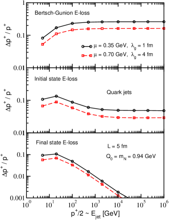
Figure 5: (Color online) Fractional energy loss for massless quark jets versus the jet energy, $E_{\rm jet}$, in cold nuclear matter of length $L=5$ fm. Two different sets of typical momentum transfer per scattering and gluon mean free path have been used for comparison: $(\mu,\lambda_{g})=(0.35$ GeV$,1$ fm$)$ and $(\mu,\lambda_{g})=(0.7$ GeV$,4$ fm$)$.

To study the radiative energy loss quantitatively, we have to identify the $|{\bf k}|$ scale, at which non-perturbative effects can become important. For cold nuclear matter, in the original work of Bertsch and Gunion Gunion:1981qs , this scale was approximated by $Q_{0}=m_{\rho}\simeq 770$ MeV. In generalized vector dominance models, the effective mass is bigger, $Q_{0}\simeq 1$ GeV, due to the contribution of the heavier vector meson states. One can also understand the appearance of form-factors in a purely partonic picture. As $|{\bf k}|\rightarrow 0$, the transverse size of the radiative gluon $A_{\perp}=1/{\bf k}^{2}$ exceeds the target parton size and the strength of the interaction of the jet + gluon system is limited. For cold nuclear matter $1/Q_{0}\leq 1/\mu\leq 1/\Lambda_{QCD}$. We take $Q_{0}=m_{N}=0.94$ GeV from the independent calculation of dynamical nuclear shadowing Vitev:2006bi ; Qiu:2004da , suggestive of partonic spots of size $\sim 0.2$ fm inside the nucleon. We implement this mass scale as follows:

$${\bf k}^{2}\rightarrow{\bf k}^{2}+Q_{0}^{2}\;\;(+x^{2}M_{q}^{2})\;.$$ (74)

The last term in Eq. (74) arises for heavy quarks and was discussed in Djordjevic:2003zk . In addition, at any fixed order the opacity expansion series is not a perfect square of a sum of amplitudes. Still, the integrands in Eqs. (69) and (70) can be represented as $(|{\bf B}_{1}|^{2}-{\bf correction})$. The requirement that the interference does not cancel differentially more than the available bremsstrahlung, induced by the medium in the absence of coherence, can be formulated as follows to any order in opacity:

$$\sum_{i=1}^{n}k^{+}\frac{dN^{g}_{(i)}}{dk^{+}d^{2}{\bf k}}\geq 0\;.$$ (75)

Eq. (75) can also used to identify and eliminate the parts of phase space where the approximations that we made are least reliable (e.g., the part of phase space where a gluon emitted in the direction opposite to the momentum transfer from the medium). To set the kinematic limits, we require that the positive gluon energy $k^{+}\geq Q_{0}$ and the gluon rapidity,

$$y_{g}=\frac{1}{2}\ln\frac{k^{+}}{k^{-}}=\frac{1}{2}\ln\frac{(k^{+})^{2}}{{\bf k}^{2}}\;,$$ (76)

be within the rapidity gap from the target to the projectile, $0\leq y_{g}\leq\ln\,(p^{+}_{\rm proj/tar}/m_{N})$. Such kinematic constraints correspond to

$$\frac{Q_{0}}{p^{+}}\leq x=\frac{k^{+}}{p^{+}}\leq 1\;,$$ (77)

$${x\,m_{N}}\leq|{\bf k}|\leq k^{+}\;.$$ (78)

We have checked that in the limit of large $p^{+}$ there is little or no sensitivity of the energy loss to a factor of two increase or decrease of the lower bounds in Eqs. (77) and (78).

In Fig. 5 we show numerical results for the fractional lightcone momentum loss $\Delta p^{+}/p^{+}$ of massless quark jets in cold nuclear matter of length $L=5$ fm. For the reference Bertsch-Gunion case, Eq. (68), in the limit of large jet energies we recover $\Delta p^{+}\propto p^{+}$. We study two sets of momentum transfers and mean free paths describing cold nuclear matter: $(\mu_{1}=0.35\;{\rm GeV},\;\lambda_{g,\,1}=1\;{\rm fm})$ and $(\mu_{2}=0.7\;{\rm GeV},\;\lambda_{g,\,2}=4\;{\rm fm})$. Clearly, the energy losses for these cases differ by close to a factor of two, indicating that $(\mu^{2}/\lambda_{g})_{1}=(\mu^{2}/\lambda_{g})_{2}$ is not a universal parameter responsible for the quenching of jets. It should be noted that for only a few scatterings in the medium with small momentum transfer $\propto\mu^{2}=0.12\;{\rm GeV}^{2}$ quarks can lose on the order of 30% of their energy.

The physically relevant case of initial-state energy loss, Eq. (69), is shown in the middle panel of Fig. 5. Destructive interference effects can lead to a large six-fold reduction of the fractional energy loss $\Delta p^{+}/p^{+}$ for $p^{+}\rightarrow\infty$. Still, qualitatively the behavior is similar to that of the Bertsch-Gunion case discussed above. For medium parameters $(\mu_{1}=0.35\;{\rm GeV}^{2}\;,\;\lambda_{g,\,1}=1\;{\rm fm})$, directly relevant to phenomenology prep , quark jets lose $\sim 5\%$ of their energy. In contrast, for final-state energy loss, shown in the bottom panel of Fig. 5, the cancellation of the radiation in the asymptotic domain is still effective, leading to $\Delta p^{+}/p^{+}\rightarrow 0$. Although there is a 30% difference between the two calculations, only in this regime of final-state radiation in cold nuclear matter may $\mu^{2}/\lambda_{g}$ be considered an approximately relevant jet quenching parameter.

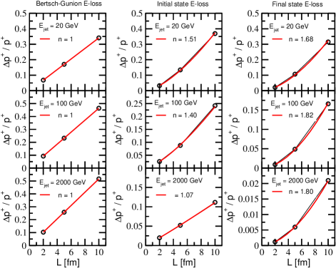
Figure 6: (Color online) Fractional energy loss for massless quark jets of $E_{\rm jet}=20$ GeV, $100$ GeV and $2000$ GeV. Three different path lengths $L=2$ fm, $5$ fm and $10$ fm were used. Power law fits indicate the system size dependence of $\Delta p^{+}/p^{+}=\Delta E_{\rm rad}/E$.

Numerical results for the path length dependence of jet energy loss in the three different regimes, Eqs. (68), (69) and (70), are presented in Fig. 6 for three jet energies, $E_{\rm jet}=20,\;100,\;2000$ GeV, respectively. By definition, the reference Bertsch-Gunion case without interference yields a linear dependence of $\Delta p^{+}/p^{+}$ on the path length $L$. Numerical calculations were carried out for three different path lengths, $L=2,\;5,\;10$ fm, and power law fits were used to extract the power index $n$ of the $\Delta p^{+}\propto L^{n}$ dependence. At large $p^{+}$ initial-state energy loss approaches a linear behavior, $n=1$, while final state energy loss shows approximately quadratic behavior, $n=2$, for static nuclear matter.

Both results have important implications for heavy ion phenomenology. Let us define the nuclear modification factor,

$$R_{AB}(p_{T}) = \frac{dN^{h}_{AB}/dyd^{2}p_{T}}{T_{AB}\;d\sigma^{h}_{pp}/dyd^{2}p_{T}}\;,$$ (79)

which is used to identify dense matter effects on parton propagation. In Eq. (79), $T_{AB}$ is the nuclear overlap function, which relates the hadron multiplicity in the many-body collision to the corresponding cross section in p+p reactions. In A+A collisions, the quadratic dependence of final-state energy loss is reduced to linear, when Bjorken expansion is taken into account, and we predict the following suppression pattern:

$$\ln R_{AA}(p_{T})=-\kappa_{AA}N_{\rm part}^{2/3}\;.$$ (80)

In Eq. (80) $N_{\rm part}$ is the total number of participants and $\kappa_{AB}$ is a microscopic coefficient, which depends on the properties of the dense latter. Initial-state energy loss, on the other hand, approaches linear dependence on the system size $\sim N_{\rm part}({\rm target})$, which can be used to predict analytically prep the centrality dependence of forward rapidity hadron suppression in p+A reactions Vitev:2006bi . Here $N_{\rm part}({\rm target})$ is the (average) number of nuclear target participants along the projectile line for a given (centrality class) impact parameter. The quantitatively different behavior of initial-state energy loss leads to the following result in p+A reactions:

$$\ln R_{pA}(p_{T})=-\kappa_{pA}N_{\rm part}({\rm target})\;.$$ (81)

Before we proceed to more differential bremsstrahlung distributions it is important to emphasize that the quadratic dependence of final-state energy loss on the size of the static medium, $\propto L^{2}$, does not imply that the magnitude of the energy loss itself is large. On the contrary, such dependence arises from the maximally efficient cancellation of the large $x=k^{+}/p^{+}$ radiation and for the same parameters of the medium, in the limit of $p^{+}\rightarrow\infty$, final-state energy loss is negligible when compared to initial-state energy loss.

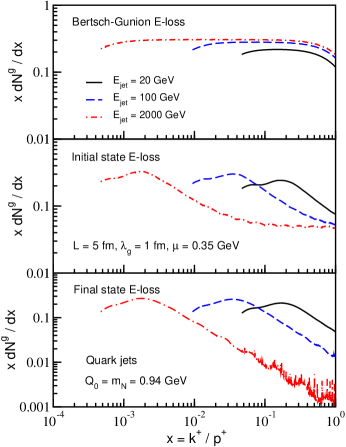
Figure 7: (Color online) Radiation intensity $xdN^{g}/dx$ for $E_{\rm jet}=20$ GeV, $100$ GeV and $2000$ GeV quark jets. Note the difference to first order in opacity in the large $x=k^{+}/p^{+}$ behavior for Bertsch-Gunion, initial-state and final-state bremsstrahlung.

One can gain insight in the energy dependence of $\Delta p^{+}$ by investigating the radiative intensity spectrum $xdN^{g}/dx$, obtained by integrating the double differential distributions Eqs. (68), (70) and (69) over ${\bf k}$ and shown in Fig 7. We have chosen $L=5$ fm $(\mu_{1}=0.35\;{\rm GeV},\;\lambda_{g,\,1}=1\;{\rm fm})$ and the same jet energies as in Fig. 6. For the Bertsch-Gunion case there is an approximately flat, up to the edge of phase space constraints, dependence of the bremsstrahlung intensity on $x$, leading to $\Delta p^{+}/p^{+}\approx{\rm const}_{BG}.$ For initial-state energy loss there is a finite cancellation of the intensity spectrum at large values of $k^{+}$, which leads to a suppressed $\Delta p^{+}/p^{+}\approx{\rm const}_{IS}$. For final-state energy loss, the spectrum is progressively more suppressed by destructive interference effects that lead to a power behavior of the intensity spectrum, $xdN^{g}/dx\propto 1/k^{+}$. Therefore, in this case, energy loss depends logarithmically on the jet energy, as first derived in Gyulassy:2000er ; Gyulassy:2000fs .

The intensity spectrum, shown in Fig 7, is also important for understanding the effect of a heavy quark mass, $M_{q}$, on the magnitude of the energy loss, $\Delta E_{\rm rad}$. Recall that the modulation of the 2D propagators and interference phases is $\propto x^{2}M_{q}^{2}$, see Eq. (74) and Ref. Djordjevic:2003zk . For the bremsstrahlung intensity, which has a negligible contribution in the region of large $x$ where the mass correction is significant, we expect that there will be no difference between $\Delta E_{\rm rad}$ for light and heavy quark. In contrast, if the kinematically allowed region in $x=k^{+}/p^{+}$ contributes equally to the radiation intensity, as in the Bertsch-Gunion case, or the cancellation of the large $x$ radiation is partial, as in the case of initial-state energy loss, then the dependence of $\Delta E_{\rm rad}$ on the heavy quark mass should remain. Numerical results for the three cases discussed in this paper are shown in Fig. 8. We used the same choice of parameters that describe cold nuclear matter in Fig. (7). Quark masses for light, charm, and bottom quarks have been set to: $M_{u,d}=0$ GeV, $M_{c}=1.3$ GeV, and $M_{b}=4.5$ GeV.

It is seen that, for final-state energy loss in cold nuclear matter, the charm quark $\Delta E_{\rm rad}$ becomes comparable to the light quark $\Delta E_{\rm rad}$ at $E_{\rm jet}\approx(p^{+}/2)=20$ GeV. For the much heavier bottom quarks, equality is reached at around 100 GeV. These results, given the crude energy binning used here to cover a very large dynamic range, $5\;{\rm GeV}<p^{+}/2<10^{6}\;{\rm GeV}$, are not inconsistent with similar findings for heavy quarks traversing a quark-gluon plasma Djordjevic:2003zk . On the other hand, for the Bertsch-Gunion case and the physically relevant case of initial-state energy loss, the mass dependence persists at any jet energy, see Fig. 8.

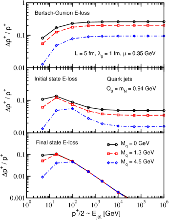
Figure 8: (Color online) Mass dependence of the fractional energy loss $\Delta E_{\rm rad}/E$ versus the jet energy, $E_{\rm jet}$. We studied massless quarks, $M_{q}=0$ GeV, charm quarks $M_{c}=1.3$ GeV and bottom quarks $M_{b}=4.5$ GeV.

The last numerical result, presented in this manuscript, is the fully differential gluon bremsstrahlung distribution $dN^{g}/dyd^{2}{\bf k}$ for select values of $x=k^{+}/p^{+}$ versus the gluon transverse momentum. We have chosen $x=0.03,0.1$ and $0.3$ to cover both small and large values of the gluon lightcone momentum fraction. Two different jet energies, $E_{jet}=100,2000$ GeV are also shown in Fig. 9. Massless quarks were used as an example in this study. The most characteristic feature of the Bertsch-Gunion energy loss is that at large values of the momentum, $|{\bf k}|$, the bremsstrahlung spectrum behaves $\sim 1/{\bf k}^{4}$. Note that this behavior is different when compared to the $\sim 1/{\bf k}^{2}$ for hard bremsstrahlung. The turnover in the growth of the spectrum at small $|{\bf k}|$ is controlled by the largest of the non-perturbative scales in the problem, in our case, $Q_{0}$. Note that there is no real difference as a function of $x$ or $E_{\rm jet}$, as expected from Eq. (51) to first order in opacity.

At the other extreme is the final-state medium-induced differential gluon distribution, see the right bottom panel of Fig. 9. The cancellation of the small $|{\bf k}|$ radiation of the basic Bertsch-Gunion term clearly becomes more effective at larger values of $x$. Given the spectrum steeply falling in $|{\bf k}|$, this cancellation is reflected in the large $x$ suppression seen in Fig. 7 and the qualitatively different behavior of the final-state $\Delta E_{\rm rad}$ when compared to QED or the Bertsch-Gunion limit. Initial-state energy loss exhibits a cancellation which, however, is limited at large values of $x$, see the middle bottom panel of Fig. 9. This explains the finite reduction of the energy loss relative to the incoherent limit of the medium-induced bremsstrahlung in QCD.

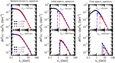
Figure 9: (Color online) Differential in the gluon transverse momentum $|{\bf k}|$ bremsstrahlung multiplicity distribution $dN^{g}/dyd^{2}{\bf k}$ for lightcone momentum fractions $x=k^{+}/p^{+}=0.03,0.1$ and $0.3$. We show for comparison quark jets of $E_{\rm jet}=100$ GeV and $2000$ GeV and the Bertsch-Gunion, initial-state and final-state spectra for comparison.

IV Discussion and conclusions

In this paper, in the framework of the reaction operator approach Gyulassy:2000er , we derived the full solution for the medium-induced gluon bremsstrahlung for asymptotic, $t=\pm\infty$, on-shell fast partons (Bertsch-Gunion) as well as partons that undergo hard scattering ($Q^{2}\gg Q_{0}^{2}\geq\mu^{2}\geq\Lambda_{QCD}^{2}$ ) to produce high-$p_{T}$ or high-$E_{T}$ particles and jets (physically relevant case). The double differential intensity spectrum, $xdN^{g}/dxd^{2}{\bf k}$, was derived as an infinite opacity series: an expansion in the correlation between the sequential multiple scatterings in the medium. Our general results are suitable for further analytic approximations and/or numerical simulations.

One of the main findings of this work is that, in contrast to final-state energy loss, the cancellation of the Bertsch-Gunion radiation for initial-state $\Delta E_{\rm rad}$ due to the non-Abelian LPM effect is less effective. While there can be a large (in our examples six-fold) reduction of the total $\Delta E_{\rm rad}$ relative to the incoherent Bertsch-Gunion case, such a cancellation does not qualitatively change the path length, $\propto L$, and the energy, $\propto E$, dependence of the radiative energy loss for finite nuclei in the case of few interactions. It is clearly the incoherent Bertsch-Gunion regime that sets the upper limit for the amount of energy loss induced by strongly interacting matter. Of the two cases relevant to hard probe physics, it is initial-state energy loss that by far dominates over final-state energy loss for the same medium parameters, such as the gluon mean free path, $\lambda_{g}$, and the squared momentum transfer, $\mu^{2}$.

The reason that final-state energy loss has been found to play a dominant role in A+A collisions is the large density of the QGP co-moving with the jet. Moreover, the effect of final-state $\Delta E_{\rm rad}$ is amplified by the steeply falling spectra of outgoing partons, $\sim 1/p_{T}^{n}$ with $n\geq 4$ Gyulassy:2003mc . This observation implies that, in a region where the flux of incoming partons is rapidly changing as a function of the $p_{T}$/$E_{T}$ of the final-state particle/jet, the cold nuclear matter $\Delta E_{\rm rad}$ can lead to a significant and observable suppression of hadron production Vitev:2006bi ; Kopeliovich:2005ym . Such regions of phase space in p+A and A+A reactions are the ones near the projectile rapidity. In such kinematic domains in the rest frame of the target nucleus the incoming partons are of almost asymptotically high energy. The knowledgeable reader can easily verify that for $p_{T}=1-2$ GeV at rapidity $y=4$, a region accessible by the STAR collaboration at RHIC Adams:2006uz , the incoming partons are of energy $E\geq 20$ TeV. Therefore, the contribution to $\Delta E$ from final-state radiative energy loss and collisional energy loss is completely negligible. In fact, due to the rapidity boost, the incoming and outgoing parton energies are very large everywhere, except in the backward region near the target rapidity. Theoretical results, derived in this manuscript, can be used to develop a more complete and consistent pQCD phenomenology of proton-nucleus collisions prep . Given the short time scale of dynamical cold nuclear matter effects, $t_{\rm col}\ll t_{\rm eq}\ll L_{T}^{QGP}$, these must also be incorporated in the description of hard processes in A+A reactions.

We also argue that a new application of cold nuclear matter-induced radiative energy loss can be related to particle production at backward rapidities. It has been established, through the measurements of the PHENIX collaboration Adler:2004eh at RHIC, that the forward rapidity hadron suppression in p+A reactions is correlated with a backward rapidity enhancement. There are no models at present that can consistently account for this effect. One possibility is that such enhancement in the inclusive particle yields may arise from the induced gluon bremsstrahlung. What makes such a scenario plausible is the fact that the gluon yield, $dN^{g}/dxd^{2}{\bf k}$, is dominated by small $x$ radiation and the destructive LPM effect cancels the small $|{\bf k}|$ part of the induced gluon spectrum. For the final-state $\Delta E_{\rm rad}$, this contribution is expected to yield an enhancement of the soft, large-angle hadrons associated with an away-side triggered jet Vitev:2005yg . For initial-state cold nuclear matter energy loss, this corresponds to gluons emitted preferentially in the backward rapidity (or near target rapidity) region, see Eq. (76). Since at moderate $k_{T}$ the power behavior of the gluon spectrum is similar to that of hard scattering, $\propto 1/k_{T}^{4}$, it may have a sizable contribution to the inclusive particle yields.

We emphasize that the results derived in this paper are applicable to both cold nuclear matter and the quark-gluon plasma. However, the physics situation of asymptotic $-\infty$, $+\infty$ jets propagating through the QGP (Bertsch-Gunion) or jets undergoing hard scattering at a finite time $t=L$, having penetrated the QGP, (initial-state) cannot be experimentally realized at present. Nevertheless, the formal radiative energy loss solutions obtained here are general enough to describe both cases of interest.

In summary, we anticipate that the results derived in this paper, in particular the ones related to initial-state cold nuclear matter radiative energy loss, will play an important role in a consistent many-body pQCD description of hard processes in high energy reactions of heavy nuclei and complement the well-developed theory and phenomenology of final-state energy loss in the quark-gluon plasma.

Appendix A Simplifying the energy loss calculation for energetic partons

In this paper we adopt the notation:

$$p^{\mu}=[p^{+},p^{-},{\bf p}]=\left[p^{0}+p^{-},p^{0}-p^{-},{\bf p}\right]\;,$$ (82)

for the lightcone momentum components. The scalar product between two 4-vectors is then given by:

$$p\cdot q=\frac{1}{2}\left(p^{+}q^{-}+p^{-}q^{+}\right)-{\bf p}\cdot{\bf q}\;.$$ (83)

The soft gluon approximation that we use implies:

$$k^{+}\ll p^{+}\;$$ (84)

for the positive lightcone momentum of the gluon relative to the lightcone momentum of the jet. Evidently, the gluon multiplicity should be dominated by small $x=k^{+}/p^{+}$ gluons, which we can verify a posteriori in all cases. The gluon intensity spectrum, however, can have contributions from the large $x$ region of phase space. For the transverse momenta we require:

$$\frac{({\bf k}-\sum_{i}{\bf q}_{i})^{2}}{k^{+}}\ll k^{+}\;.$$ (85)

This constraint implies that at the emission vertex the transverse momentum ${\bf k}-\sum_{i}{\bf q}_{i}$ of the gluon is small and the large transverse momenta ${\bf k}$ are accumulated via multiple scattering, which can be large angle. Finally,

$$\frac{({\bf k}-\sum_{i}{\bf q}_{i})^{2}}{p^{+}}\approx 0\ll\frac{({\bf k}-\sum_{i}{\bf q}_{i})^{2}}{k^{+}}\;,$$ (86)

and such terms are neglected. The polarization vector for the physical final-state gluon is given by

$$\epsilon(k)=\left[\,0,2\frac{\epsilon_{\perp}\cdot{\bf k}}{k+},\epsilon_{\perp}\,\right]\;\;,$$ (87)

so that $\epsilon(k)\cdot k=0$. With $n$ momentum transfers from the medium and the approximations outlined in Eqs. (84) - (86), the kinematic part of the gluon emission vertex reads:

$$\Gamma_{i_{1}\cdots i_{n}}\approx 2p^{+}(k^{+})^{n-1}\epsilon_{\perp}\cdot({\bf k}-{\bf q}_{i_{1}}-\cdots-{\bf q}_{i_{n}})\;.$$ (88)

The color factor, associated with Eq. (88), is $(-f^{ca_{n}d_{n}})(-f^{d_{n}a_{n-1}d_{n-1}})\cdots(-f^{d_{2}a_{1}d_{1}})ig_{s}\,t_{d_{1}}$. Here, $t_{d_{1}}\equiv d_{1}$ is the color matrix at the emission vertex. Thus, a common factor $-2ig_{s}\epsilon_{\perp}\cdot(\cdots)$ can be factored out from all amplitudes.

While the integrals over the longitudinal position of the scattering centers, $z_{i}$, have to be taken explicitly, a major simplification at the level of squared amplitudes occurs when we consider the average over the corresponding impact parameters ${\bf b}_{i}={\bf x}_{i}-{\bf x}_{0}$. This average is done in the local rest frame of the medium containing colored scattering centers. For a scattering center, $i$, that appears in a direct interaction the impact parameter average takes the form:

$$\langle\cdots\rangle_{A_{\perp}} = \langle\cdots\int\frac{d^{2}{\bf b}_{i}}{A_{\perp}}\,(-i)\int\frac{d^{2}{\bf q}_{i}}{(2\pi)^{2}}\,{\cal A}_{el}(0,{\bf q}_{i})\,e^{-i{\bf q}_{i}\cdot{\bf b}_{i}}\,(+i)\int\frac{d^{2}{\bf q}_{i}^{\prime}}{(2\pi)^{2}}\,{\cal A}_{el}^{*}(0,{\bf q}_{i}^{\prime})\,e^{+i{\bf q}_{i}^{\;\prime}\cdot{\bf b}_{i}}\;\cdots\rangle\;$$

$$= \cdots\int\frac{d^{2}{\bf q}_{i}}{(2\pi)^{2}}\,\frac{d^{2}{\bf q}_{i}^{\prime}}{(2\pi)^{2}}\frac{(2\pi)^{2}\delta^{2}({\bf q}_{i}-{\bf q}_{i}^{\prime})}{A_{\perp}}{\cal A}_{el}^{*}({\bf q}_{i}^{\prime}){\cal A}_{el}({\bf q}_{i})\;\cdots=\cdots\frac{\sigma_{el}}{A_{\perp}}\int\frac{d^{2}{\bf q}_{i}}{(2\pi)^{2}}\left[\frac{1}{\sigma_{el}}\frac{d\sigma_{el}}{d^{2}{\bf q}_{i}}\right]\,\;\int d^{2}{\bf q}_{i}^{\prime}\delta^{2}({\bf q}_{i}-{\bf q}_{i}^{\prime})\;\cdots\,\;\;,$$

which constrains the transverse momentum exchanges ${\bf q}_{i}={\bf q}_{i}^{\prime}$ to be equal in the amplitude and its conjugate. For a double-Born interaction:

$$\langle\cdots\rangle_{A_{\perp}} = \langle\cdots\int\frac{d^{2}{\bf b}_{i}}{A_{\perp}}\,(-i)\int\frac{d^{2}{\bf q}_{i}}{(2\pi)^{2}}\,{\cal A}_{el}(0,{\bf q}_{i})\,e^{-i{\bf q}_{i}\cdot{\bf b}_{i}}\,(-i)\int\frac{d^{2}{\bf q}_{i}^{\prime}}{(2\pi)^{2}}\,{\cal A}_{el}(0,{\bf q}_{i}^{\prime})\,e^{-i{\bf q}_{i}^{\;\prime}\cdot{\bf b}_{i}}\;\cdots\rangle\;$$ (90)

$$= \cdots(-1)\int\frac{d^{2}{\bf q}_{i}}{(2\pi)^{2}}\,\frac{d^{2}{\bf q}_{i}^{\prime}}{(2\pi)^{2}}\frac{(2\pi)^{2}\delta^{2}({\bf q}_{i}+{\bf q}_{i}^{\prime})}{A_{\perp}}{\cal A}_{el}(0,{\bf q}_{i}){\cal A}_{el}(0,{\bf q}_{i}^{\prime})\;\cdots\;\;$$

$$= \cdots(-1)\frac{\sigma_{el}}{A_{\perp}}\int\frac{d^{2}{\bf q}_{i}}{(2\pi)^{2}}\,\left[\frac{1}{\sigma_{el}}\frac{d\sigma_{el}}{d^{2}{\bf q}_{i}}\right]\;\int d^{2}{\bf q}_{i}\delta^{2}({\bf q}_{i}+{\bf q}_{i}^{\prime})\;\cdots\,\;\;.$$

The momentum transfers are constrained here to be equal and opposite. In Eq. (90) we have used ${\cal A}_{el}(0,{\bf q}_{i})={\cal A}_{el}^{\star}(0,{\bf q}_{i})$ and ${\cal A}_{el}(0,{\bf q}_{i})={\cal A}_{el}(0,-{\bf q}_{i})$.

Appendix B Amplitude iteration technique to second order in opacity for on-shell partons

We illustrate the iteration of gluon emission amplitudes to second order in opacity and calculate the Bertsch-Gunion case for direct comparison to the general gluon emission result for soft scatterings Eq. (51). One should first recall that for the Bertsch-Gunion case

$$G_{0}={\bf 0}\;,$$ (91)

since the asymptotic on-shell quarks do not radiate without the medium-induced acceleration. For the two rank 1 classes, we apply once the direct and virtual insertion operators, $\hat{D}_{1}$ from Eq. (17) and $\hat{V}_{1}$ from Eq. (27), to the incoming parton, Eq. (91), and obtain:

$$D_{1}G_{0} = -{\bf B}_{1}\,e^{i\omega_{0}z_{1}}\,[c,a_{1}]\;\;,$$ (92)

$$V_{1}G_{0} = -\frac{C_{A}}{2}\,{\bf B}_{1}\,e^{i\omega_{0}z_{1}}\,c\;\;.$$ (93)

We note that the results are simple since only the new color current ${\bf B}_{1}$ contributes in the absence of a non-zero initial gluon amplitude.

To second order in opacity, we build upon the amplitudes from Eqs. (92) and (93). Some of the rank 2 classes are obtained from rank 1 through relabeling, i.e. $D_{2}G_{0}\equiv D_{1}G_{0}(1\rightarrow 2),\;V_{2}G_{0}\equiv V_{1}G_{0}(1\rightarrow 2)$. The rest are readily derived from Eqs. (92) and (93) through our iteration scheme Eqs. (17) and (27):

$$D_{2}D_{1}G_{0} = -{\bf B}_{1}\,e^{i\omega_{0}z_{1}}\,a_{2}[c,a_{1}]-{\bf B}_{2}\,e^{i\omega_{0}z_{2}}\,[c,a_{2}]a_{1}$$ (94)

$$-{\bf B}_{2(12)}\,e^{i(\omega_{0}z_{2}-\omega_{2}z_{21})}\,[[c,a_{2}],a_{1}]\;\;,$$

$$V_{2}D_{1}G_{0} = +\frac{C_{R}+C_{A}}{2}\,{\bf B}_{1}\,e^{i\omega_{0}z_{1}}\,[c,a_{1}]$$ (95)

$$-\frac{C_{A}}{2}\,{\bf B}_{2}\,e^{i\omega_{0}z_{2}}\,ca_{1}$$

$$+{\bf B}_{2(12)}\,e^{i(\omega_{0}z_{2}-\omega_{2}z_{21})}\,a_{2}[[c,a_{2}],a_{1}]\;\;,$$

$$D_{2}V_{1}G_{0} = -\frac{C_{A}}{2}\,{\bf B}_{1}\,e^{i\omega_{0}z_{1}}\,a_{2}c+\frac{C_{R}}{2}\,{\bf B}_{2}\,e^{i\omega_{0}z_{2}}\,[c,a_{2}]$$ (96)

$$-\frac{C_{A}}{2}\,{\bf B}_{2(12)}\,e^{i(\omega_{0}z_{2}-\omega_{2}z_{21})}\,[c,a_{2}]\;\;,$$

$$V_{2}V_{1}G_{0} = +\frac{C_{A}(C_{R}+C_{A})}{4}\,{\bf B}_{1}\,e^{i\omega_{0}z_{1}}\,c$$ (97)

$$+\frac{C_{R}C_{A}}{4}\,{\bf B}_{2}\,e^{i\omega_{0}z_{2}}\,c$$

$$-\frac{C^{2}_{A}}{4}\,{\bf B}_{2(12)}\,e^{i(\omega_{0}z_{2}-\omega_{2}z_{21})}\,c\;\;.$$

With this explicit construction of the relevant classes of diagrams, we can compute the differential gluon emission up to second order in the opacity expansion.

A necessary side step in the brute force approach is the evaluation of the color factors using the techniques in Refs. Cvitanovic:1976am ; Gyulassy:1999zd . We denote by $C_{R}$ the quadratic Casimir of the representation of the incident parton. For SU($N_{c}$), following the standard normalization for the generators we have

$$C_{F}={N_{c}^{2}-1\over 2N_{c}},\qquad C_{A}=N_{c}\;.$$ (98)

We recall that in our notation $T_{c}\equiv c$ for brevity. In the absence of interactions we have only one color matrix associated with the gluon emission vertex from a hard scatter,

$${\cal C}^{(0)}_{1}=c\;,$$ (99)

with

$${{\rm Tr}}\;{\cal C}^{(0)\dagger}_{1}{\cal C}^{(0)}_{1}=C_{R}D_{R}\;.$$ (100)

To first order in opacity we have to consider the following color factors

$${\cal C}^{(1)}_{1}=ca_{1}\;,\quad{\cal C}^{(1)}_{2}=\left[c,a_{1}\right]\;,\quad{\cal C}^{(1)}_{3}=a_{1}c\;,$$ (101)

with

$${{\rm Tr}}\;{\cal C}^{(1)\dagger}_{1}{\cal C}^{(1)}_{1}=C_{R}^{2}D_{R}\;,\quad{\cal C}^{(1)\dagger}_{2}{\cal C}^{(1)}_{2}=C_{R}C_{A}D_{R}\;,$$

$${{\rm Tr}}\;{\cal C}^{(1)\dagger}_{3}{\cal C}^{(1)}_{3}=C_{R}^{2}D_{R}\;,$$

$${{\rm Tr}}\;{\cal C}^{(1)\dagger}_{1}{\cal C}^{(1)}_{2}=\frac{C_{A}}{2}C_{R}D_{R}\;,\quad$$

$${{\rm Tr}}\;{\cal C}^{(1)\dagger}_{1}{\cal C}^{(1)}_{3}=\left(C_{R}-\frac{1}{2}C_{A}\right)C_{R}D_{R}\;,$$

$${{\rm Tr}}\;{\cal C}^{(1)\dagger}_{2}{\cal C}^{(1)}_{3}=\frac{C_{A}}{2}C_{R}D_{R}\;.$$ (102)

To second order in opacity we have:

$${\cal C}^{(2)}_{1}=a_{2}a_{1}c\;,\quad{\cal C}^{(2)}_{2}=a_{2}\left[c,a_{1}\right]\;,$$

$${\cal C}^{(2)}_{3}=\left[c,a_{2}\right]a_{1}\;,\quad{\cal C}^{(2)}_{4}=c\,a_{2}a_{1}\;,\quad$$

$${\cal C}^{(2)}_{5}=\left[\left[c,a_{2}\right],a_{1}\right]\;.$$ (103)

The traces over the color factors yield:

$${{\rm Tr}}\,{\cal C}_{1}^{(2)\dagger}{\cal C}^{(2)}_{1}={{\rm Tr}}\,{\cal C}_{4}^{(2)\dagger}{\cal C}^{(2)}_{4}=C^{3}_{R}D_{R}\;,\quad$$

$${{\rm Tr}}\,{\cal C}^{(2)\dagger}_{2}{\cal C}^{(2)}_{2}={{\rm Tr}}\,{\cal C}^{(2)\dagger}_{3}{\cal C}^{(2)}_{3}=C_{A}C^{2}_{R}D_{R}\;,\quad$$

$${{\rm Tr}}\,{\cal C}^{(2)\dagger}_{5}{\cal C}^{(2)}_{5}=C^{2}_{A}C_{R}D_{R}\;,$$

$${{\rm Tr}}\,{\cal C}^{(2)\dagger}_{1}{\cal C}^{(2)}_{2}=-{{\rm Tr}}\,{\cal C}^{(2)\dagger}_{3}{\cal C}^{(2)}_{4}=-\frac{1}{2}C_{A}C^{2}_{R}D_{R}\;,\quad$$

$${{\rm Tr}}\,{\cal C}^{(2)\dagger}_{1}{\cal C}^{(2)}_{3}=-{{\rm Tr}}\,{\cal C}^{(2)\dagger}_{2}{\cal C}^{(2)}_{4}$$

$$\hskip 54.06006pt=-\frac{1}{2}\left(C_{R}-\frac{1}{2}C_{A}\right)C_{A}C_{R}D_{R}\;,$$

$${{\rm Tr}}\,{\cal C}^{(2)\dagger}_{1}{\cal C}^{(2)}_{4}=\left(C_{R}-\frac{1}{2}C_{A}\right)^{2}C_{R}D_{R}\;,$$

$${{\rm Tr}}\,{\cal C}^{(2)\dagger}_{1}{\cal C}^{(2)}_{5}=0\;,$$

$${{\rm Tr}}\,{\cal C}^{(2)\dagger}_{2}{\cal C}^{(2)}_{3}={{\rm Tr}}\,{\cal C}^{(2)\dagger}_{2}{\cal C}^{(2)}_{5}=-{{\rm Tr}}\,{\cal C}^{(2)\dagger}_{4}{\cal C}^{(2)}_{5}$$

$$\hskip 54.06006pt=-\frac{1}{4}C^{2}_{A}C_{R}D_{R}\;,\quad$$

$${{\rm Tr}}\,{\cal C}^{(2)\dagger}_{3}{\cal C}^{(2)}_{5}=\frac{1}{2}C^{2}_{A}C_{R}\;,\quad$$ (104)

Although some of the color factors, such as ${\cal C}^{(1)}_{3}$ and ${\cal C}^{(2)}_{4}$, do not appear in the amplitudes listed above, these will prove useful in the calculation of the realistic case of incoming partons that undergo hard scattering to produce final-state jets.

To first order in opacity, the radiation from either quark or gluon jets reads:

$$k^{+}\frac{N^{(1)}_{g}(BG)}{dk^{+}d^{2}{\bf k}} \propto \frac{1}{D_{R}}\,\left\langle\;{\rm Tr}\left[(D_{1}G_{0})^{\dagger}D_{1}G_{0}\right.\right.$$ (105)

$$\hskip 22.76228pt\left.\left.+((G_{0})^{\dagger}V_{1}G_{0}+h.c.)\right]\;\right\rangle\;.\qquad$$

In Eq. (105), $\left\langle\cdots\right\rangle$ denotes the average over the momentum transfers from the medium. Including the phase space factor, the strong coupling constant $\alpha_{s}$ and integrating over the longitudinal position of the scattering centers we find:

$$k^{+}\frac{N^{(1)}_{g}(BG)}{dk^{+}d^{2}{\bf k}} = \frac{C_{R}\alpha_{s}}{\pi^{2}}\int_{0}^{L}\frac{d\Delta z_{1}}{\lambda_{g}(z_{1})}\;\int d^{2}{\bf q}_{1}\;$$ (106)

$$\hskip 28.45274pt\times\frac{1}{\sigma_{el}(z_{1})}\frac{d\sigma_{el}}{d^{2}{\bf q}_{1}}\left[\;|{\bf B}_{1}|^{2}\;\right]\;.\;\;\qquad$$

Here, we recover the Bertsch-Gunion result to one scattering center Gunion:1981qs and show that it is equivalent to first order in opacity. One important difference between the initial- and/or final-state radiation and on-shell jets is that in the latter cases the first order in opacity does not lead to any interference/coherence effects.

The first non-trivial correction to the Bertsch-Gunion result can also be directly calculated. Using the amplitudes, Eqs. (92) - (97), and the calculated color factors, Eqs. (101) - (104), we find:

$$k^{+}\frac{N^{(2)}_{g}(BG)}{dk^{+}d^{2}{\bf k}} \propto \frac{1}{D_{R}}\,\left\langle\;{\rm Tr}\left[\,(D_{2}D_{1}G_{0})^{\dagger}D_{2}D_{1}G_{0}\right.\right.$$ (107)

$$+\;((D_{2}G_{0})^{\dagger}D_{2}V_{1}G_{0}+{\rm h.c.})$$

$$+\;((D_{1}G_{0})^{\dagger}V_{2}D_{1}G_{0}+{\rm h.c.})$$

$$+\;((G_{0})^{\dagger}V_{2}V_{1}G_{0}+{\rm h.c.})$$

$$\left.\left.+\;((V_{2}G_{0})^{\dagger}V_{1}G_{0}+{\rm h.c.})\,\right]\;\right\rangle\;.$$

The final result for the first non-trivial coherence correction reads:

$$k^{+}\frac{N^{(2)}_{g}(BG)}{dk^{+}d^{2}{\bf k}} = \frac{C_{R}\alpha_{s}}{\pi^{2}}\int_{0}^{L}\frac{d\Delta z_{1}}{\lambda_{g}(z_{1})}\int_{0}^{L-\Delta z_{1}}\frac{d\Delta z_{2}}{\lambda_{g}(z_{2})}$$

$$\times\int{d^{2}{\bf q}_{1}}\frac{1}{\sigma_{el}(z_{1})}\frac{d\sigma_{el}}{d^{2}{\bf q}_{1}}\;\int d^{2}{\bf q}_{2}\;\frac{1}{\sigma_{el}(z_{2})}\frac{d\sigma_{el}}{d^{2}{\bf q}_{2}}$$

$$\ \times\left[\;|{\bf B}_{2(12)}|^{2}-|{\bf B}_{1}|^{2}+2{\bf B}_{2}\cdot{\bf B}_{2(12)}\cos(\omega_{2}z_{21})\;\right]\;.$$

In a medium with no sharp boundaries we can extend the integration limits as follows, $z(0)\rightarrow-\infty$, $z(L)\rightarrow+\infty$. The disappearance of the interactions is guaranteed by $\lambda_{g}(z_{i})\rightarrow\infty$ as $\rho(z_{i})\rightarrow 0$. Direct comparison to the full recurrence solution, Eq. (51), can now be made with consistent results, as expected.

Appendix C Amplitude iteration technique to second order in opacity for initial-state radiation

The case of initial-state energy loss, as emphasized in the general derivation section, differs from the full Bertsch-Gunion solution by the presence of the additional hard scatter at position $L$. While the $t=-\infty$ state for the incoming on-shell parton remains the same, the hard acceleration yields an additional term:

$${H}=\left(-\frac{1}{2}\right)^{{N}_{v}({\cal A}_{i_{1}\cdots i_{n}})}\,{\bf H}e^{i\omega_{0}z_{L}}\;cT_{el}({\cal A}_{i_{1}\cdots i_{n}})\;.\quad$$ (109)

In the absence of soft interactions,

$$G_{0}+H={\bf H}e^{i\omega_{0}z_{L}}\;c\;\;.$$ (110)

The dependence of $H$ on the sequence of interactions preceding the hard scatter is implicit on our notation. If we want to explicitly verify the general result to second order in opacity, we need to calculate only a few additional terms relative to Appendix B. The relevant amplitudes are modified as follows,

$$D_{1}G_{0}+H = -{\bf B}_{1}\,e^{i\omega_{0}z_{1}}\,[c,a_{1}]+{\bf H}e^{i\omega_{0}z_{L}}\,ca_{1}\;\;,\qquad$$ (111)

$$V_{1}G_{0}+H = -\frac{C_{A}}{2}\,{\bf B}_{1}\,e^{i\omega_{0}z_{1}}\,c-\frac{C_{R}}{2}{\bf H}e^{i\omega_{0}z_{L}}\,c\;\;,\qquad$$ (112)

and

$$D_{2}D_{1}G_{0}+H = -{\bf B}_{1}\,e^{i\omega_{0}z_{1}}\,a_{2}[c,a_{1}]$$ (113)

$$-{\bf B}_{2}\,e^{i\omega_{0}z_{2}}\,[c,a_{2}]a_{1}$$

$$-{\bf B}_{2(12)}\,e^{i(\omega_{0}z_{2}-\omega_{2}z_{21})}\,[[c,a_{2}],a_{1}]$$

$$+{\bf H}e^{i\omega_{0}z_{L}}\,ca_{2}a_{1}\;\;,$$

$$V_{2}D_{1}G_{0}+H = +\frac{C_{R}+C_{A}}{2}\,{\bf B}_{1}\,e^{i\omega_{0}z_{1}}\,[c,a_{1}]$$ (114)

$$-\frac{C_{A}}{2}\,{\bf B}_{2}\,e^{i\omega_{0}z_{2}}\,ca_{1}$$

$$+{\bf B}_{2(12)}\,e^{i(\omega_{0}z_{2}-\omega_{2}z_{21})}\,a_{2}[[c,a_{2}],a_{1}]$$

$$-\frac{C_{R}}{2}{\bf H}e^{i\omega_{0}z_{L}}\,ca_{1}\;\;,$$

$$D_{2}V_{1}G_{0}+H = -\frac{C_{A}}{2}\,{\bf B}_{1}\,e^{i\omega_{0}z_{1}}\,a_{2}c$$ (115)

$$+\frac{C_{R}}{2}\,{\bf B}_{2}\,e^{i\omega_{0}z_{2}}\,[c,a_{2}]$$

$$-\frac{C_{A}}{2}\,{\bf B}_{2(12)}\,e^{i(\omega_{0}z_{2}-\omega_{2}z_{21})}\,[c,a_{2}]$$

$$-\frac{C_{R}}{2}{\bf H}e^{i\omega_{0}z_{L}}\,ca_{2}\;\;,$$

$$V_{2}V_{1}G_{0}+H = +\frac{C_{A}(C_{R}+C_{A})}{4}\,{\bf B}_{1}\,e^{i\omega_{0}z_{1}}\,c$$ (116)

$$+\frac{C_{R}C_{A}}{4}\,{\bf B}_{2}\,e^{i\omega_{0}z_{2}}\,c$$

$$-\frac{C^{2}_{A}}{4}\,{\bf B}_{2(12)}\,e^{i(\omega_{0}z_{2}-\omega_{2}z_{21})}\,c$$

$$+\frac{C_{R}^{2}}{4}{\bf H}e^{i\omega_{0}z_{L}}\,c\;\;,$$

in comparison to Eqs. (92) - (97). Having also calculated the color factors for this case in Appendix B, we obtain

$$k^{+}\frac{N^{(2)}_{g}(IS)}{dk^{+}d^{2}{\bf k}} \propto \frac{1}{D_{R}}\,\left\langle\;{\rm Tr}\left[\,(D_{2}D_{1}G_{0}+H)^{\dagger}(D_{2}D_{1}G_{0}+H)+((D_{2}G_{0}+H)^{\dagger}(D_{2}V_{1}G_{0}+H)+{\rm h.c.})\right.\right.$$ (117)

$$+\;((D_{1}G_{0}+H)^{\dagger}(V_{2}D_{1}G_{0}+H)+{\rm h.c.})+((G_{0}+H)^{\dagger}(V_{2}V_{1}G_{0}+H)+{\rm h.c.})$$

$$\left.\left.+((V_{2}G_{0}+H)^{\dagger}(V_{1}G_{0}+H)+{\rm h.c.})\,\right]\;\right\rangle\;.$$

Evaluating the additional terms, arising from the interference of the hard gluon bremsstrahlung with the multiple Bertsch-Gunion sources, and showing explicitly that the term $\propto{\bf H}^{2}$ cancels, we obtain:

$$k^{+}\frac{N^{(1)}_{g}(IS)}{dk^{+}d^{2}{\bf k}} = \frac{C_{R}\alpha_{s}}{\pi^{2}}\int_{0}^{L}\frac{d\Delta z_{1}}{\lambda_{g}(z_{1})}\int{d^{2}{\bf q}_{1}}\frac{1}{\sigma_{el}(z_{1})}\frac{d\sigma_{el}}{d^{2}{\bf q}_{1}}\;\left[\;|{\bf B}_{1}|^{2}\;-2{\bf H}\cdot{\bf B}_{1}\cos(\omega_{0}z_{L1})\right]\;.\qquad$$ (118)

$$k^{+}\frac{N^{(2)}_{g}(IS)}{dk^{+}d^{2}{\bf k}} = \frac{C_{R}\alpha_{s}}{\pi^{2}}\int_{0}^{L}\frac{d\Delta z_{1}}{\lambda_{g}(z_{1})}\int_{0}^{L-\Delta z_{1}}\frac{d\Delta z_{2}}{\lambda_{g}(z_{2})}\int{d^{2}{\bf q}_{1}}\frac{1}{\sigma_{el}(z_{1})}\frac{d\sigma_{el}}{d^{2}{\bf q}_{1}}\;\int d^{2}{\bf q}_{2}\;\frac{1}{\sigma_{el}(z_{2})}\frac{d\sigma_{el}}{d^{2}{\bf q}_{2}}\;\left[\;|{\bf B}_{2(12)}|^{2}\right.$$ (119)

$$\;\left.\;-|{\bf B}_{1}|^{2}+2{\bf B}_{2}\cdot{\bf B}_{2(12)}\cos(\omega_{2}z_{21})-2{\bf H}\cdot{\bf B}_{2(12)}\cos(\omega_{0}z_{L2}+\omega_{2}z_{21})+2{\bf H}\cdot{\bf B}_{1}\cos(\omega_{0}z_{L1})\;\right]\;.\qquad$$

These results coincide with the general opacity expansion series for initial-state medium-induced non-Abelian bremsstrahlung, see Eq. (63).

References

• (1) M. Gyulassy, I. Vitev, X. N. Wang and B. W. Zhang, nucl-th/0302077, in R. C. Hwa and X. N. Wang editors, Quark-Gluon Plasma III, 123 (2004).
• (2) A. Kovner and U. A. Wiedemann, hep-ph/0304151, in R. C. Hwa and X. N. Wang editors, Quark-Gluon Plasma III, 192 (2004).
• (3) R. Baier, D. Schiff and B. G. Zakharov, Ann. Rev. Nucl. Part. Sci.  50, 37 (2000).
• (4) I. Vitev, J. Phys. G 30, S791 (2004); references therein.
• (5) A. Majumder, nucl-th/0702066; references therein.
• (6) I. Arsene et al. [BRAHMS Collaboration], Phys. Rev. Lett.  93, 242303 (2004).
• (7) J. Adams et al. [STAR Collaboration], Phys. Rev. Lett.  97, 152302 (2006).
• (8) V. Guzey, M. Strikman and W. Vogelsang, Phys. Lett.  B 603, 173 (2004).
• (9) J. W. Qiu and I. Vitev, Phys. Lett. B 632, 507 (2006).
• (10) I. Vitev, T. Goldman, M. B. Johnson and J. W. Qiu, Phys. Rev. D  74, 054010 (2006).
• (11) J. F. Gunion and G. Bertsch, Phys. Rev. D 25, 746 (1982).
• (12) L. D. Landau and I. Pomeranchuk, Dokl. Akad. Nauk Ser. Fiz.  92, 535 (1953);
• (13) A. B. Migdal, Phys. Rev.  103, 1811 (1956).
• (14) I. Vitev, “Are jets quenched in cold nuclei”, in preparation.
• (15) M. G. Mustafa, Phys. Rev.  C 72, 014905 (2005).
• (16) A. Adil, M. Gyulassy, W. A. Horowitz and S. Wicks, Phys. Rev.  C 75, 044906 (2007).
• (17) J. D. Jackson, “Classical electrodynamics”, John Wiley & Sons, Inc., New York (1998).
• (18) M. Gyulassy, P. Levai and I. Vitev, Nucl. Phys. B 594, 371 (2001).
• (19) M. Gyulassy, P. Levai and I. Vitev, Phys. Rev. Lett.  85, 5535 (2000).
• (20) M. Gyulassy, P. Levai and I. Vitev, Phys. Rev. D 66, 014005 (2002).
• (21) A. Adil and I. Vitev, Phys. Lett.  B 649, 139 (2007).
• (22) H. Zhang, Z. Kang and E. Wang, hep-ph/0609159.
• (23) M. Djordjevic and M. Gyulassy, Nucl. Phys. A 733, 265 (2004).
• (24) B. Z. Kopeliovich, J. Nemchik, I. K. Potashnikova, M. B. Johnson and I. Schmidt, Phys. Rev.  C 72, 054606 (2005).
• (25) S. S. Adler et al. [PHENIX Collaboration], Phys. Rev. Lett.  94, 082302 (2005).
• (26) I. Vitev, Phys. Lett. B 630, 78 (2005).
• (27) P. Cvitanovic, Phys. Rev.  D 14, 1536 (1976).
• (28) M. Gyulassy, P. Levai and I. Vitev, Nucl. Phys.  B 571, 197 (2000).