Squark Pair Production in the MSSM with Explicit CP Violation

Ahmet T. Alana, Kerem Cankoçakb and Durmuş A. Demirc aDepartment of Physics, Abant Izzet Baysal University, Turkey, TR14280 bDepartment of Physics, Mug̃la University, Turkey, TR48000 c Department of Physics, Izmir Institute of Technology, IZTECH, Turkey, TR35430
Abstract

We analyze effects of the CP-odd soft phases in the MSSM on the pair-productions of colored superpartners in $p\,p$ collisions at the LHC energies. We find that, among all pair-production processes, those of the scalar quarks in the first and second generations are particularly sensitive to the CP-odd phases, more precisely, to the phases of the gluinos and neutralinos. We compute pair-production cross sections, classify various production modes according to their dependencies on the gluino and neutralino phases, perform a detailed numerical analysis to determine individual as well as total cross sections, and give a detailed discussion of EDM bounds. We find that pair-productions of first and second generation squarks serve as a viable probe of the CP violation sources in the gaugino sector of the theory even if experiments cannot determine chirality, flavor and electric charge of the squarks produced.

preprint: IZTECH-P01/2007  October 2007

I Introduction and Motivation

Supersymmetric extension of the standard model of particle physics (SM) is one of the most plausible scenarios for new physics to be discovered at the LHC. Supersymmetry is to be a blatantly broken symmetry of nature as indicated by negative searches at LEP (and also at Tevatron). This breaking should occur softly $i.e.$ in a way not regenerating the quadratic divergences. The soft-breaking sector of the theory consists of a number of dimensionful parameters (see the review volume Chung:2003fi ): the gaugino masses $M_{\widetilde{g},\widetilde{W},\widetilde{B}}$, trilinear couplings ${\bf Y_{u,d,e}^{A}}$ and sparticle masses $M_{H_{u}}^{2}\cdots{\bf M_{E}}^{2}$. These parameters, forming up the soft-breaking lagrangian

$\displaystyle-{\bf L}_{soft}$ $\displaystyle=$ $\displaystyle\frac{1}{2}\left[M_{\widetilde{g}}\lambda_{\widetilde{g}}^{a}\lambda_{\widetilde{g}}^{a}+M_{\widetilde{W}}\lambda_{\widetilde{W}}^{i}\lambda_{\widetilde{W}}^{i}+M_{\widetilde{B}}\lambda_{\widetilde{B}}\lambda_{\widetilde{B}}+\mbox{h.c.}\right]$ (1)
$\displaystyle+$ $\displaystyle M_{H_{d}}^{2}H_{d}^{\dagger}H_{d}+M_{H_{u}}^{2}H_{u}^{\dagger}H_{u}-\left[\mu B{H}_{d}\cdot{H}_{u}+\mbox{h.c.}\right]$
$\displaystyle+$ $\displaystyle\left[\widetilde{Q}\cdot{H}_{u}{\bf Y_{u}^{A}}\widetilde{U}^{c}+{H}_{d}\cdot\widetilde{Q}{\bf Y_{d}^{A}}\widetilde{D}^{c}+{H}_{d}\cdot\widetilde{L}{\bf Y_{e}^{A}}\widetilde{E}^{c}+\mbox{h.c.}\right]$
$\displaystyle+$ $\displaystyle\widetilde{Q}^{\dagger}{\bf M_{Q}}^{2}\widetilde{Q}+\widetilde{U}^{c\dagger}{\bf M_{U}}^{2}\widetilde{U}^{c}+\widetilde{D}^{c\dagger}{\bf M_{D}}^{2}\widetilde{D}^{c}+\widetilde{L}^{\dagger}{\bf M_{L}}^{2}\widetilde{L}+\widetilde{E}^{c\dagger}{\bf M_{E}}^{2}\widetilde{E}^{c}$

are the main goal of measurements to be carried out at the LHC. The $\mu$ parameter, gaugino masses, trilinear couplings and off-diagonal entries of the squark and slepton masses are the sources of CP violation beyond the SM. Likewise, sfermion mass-squareds and trilinear couplings are sources of flavor violation beyond the SM.

The experiments at the LHC are expected to confirm massive superpartners if nature is supersymmetric around Fermi energies. Clearly, if measurements at the LHC will suffice to construct the soft-breaking lagrangian (1) or if measurements will ever lead to a unique supersymmetric model requires a dedicated analysis of collider signals and model predictions nima (see also the dedicated review volume pape ). A further question concerns role of the soft masses in CP and flavor violating phenomena, and this can be achieved after a full experimentation of various meson decays and mixings flavor-cp . In this work, we intend to contribute this enormous project by a detailed analysis of squark pair production at $pp$ collisions. These processes have been analyzed in the past cross ; cross1 (with increasing precision in Beenakker:1996ch ; Beenakker3 ; tilman ) by considering only the (dominant) SUSY QCD contributions. Moreover, spin asymmetries have been analyzed in wyler . Our motivation for and certain salient features of squark pair-production processes can be summarized as follows:

  1. 1.

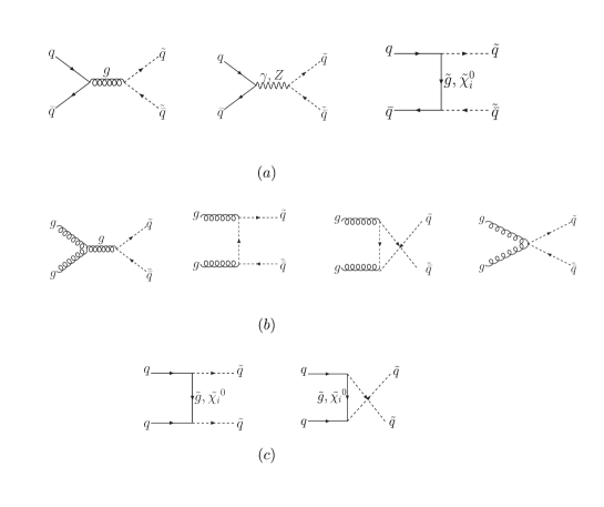
    Squarks and gluinos are expected to be produced copiously (via several channels as depicted in Fig. 1 for a generic squark flavor $\widetilde{q}$). This is not the case for leptons, neutralinos and charginos whose direct productions are initiated by quark–anti-quark annihilation, only.

  2. 2.

    Squark pair production is dominated by SUSY QCD contributions $i.e.$ gluino exchange. However, it is important to consider also the exchange of electroweak gauginos since interference of gluino– and gaugino–mediated amplitudes can be sizeable.

  3. 3.

    As illustrated in Fig. 1, $\widetilde{q}\widetilde{q}^{\star}$ production receives significant SM contributions from photon, $Z$ and gluon exchanges in the $s$-channel. In addition, there are purely supersymmetric contributions from $t$-channel gluino and neutralino exchanges. The whole process is $p$-wave. The dependence on the supersymmetric CP-odd phases involves only the difference between neutralino phases, in particular, there is no dependence on the phase of the gluino mass. The reason is that the vertices connecting to $\widetilde{q}$ and $\widetilde{q}^{\star}$ interfere destructively due to complex conjugation.

    The production of $\widetilde{q}\widetilde{q}$ pairs proceeds solely with the sparticle mediation, as shown in Fig.1 part (c). This purely supersymmetric amplitude describes an $s$-wave scattering, and thus, near the two-squark threshold $\widetilde{q}\widetilde{q}$ events can dominate $\widetilde{q}\widetilde{q}^{\star}$ ones. Moreover, unlike $\widetilde{q}\widetilde{q}^{\star}$ production amplitude, $\widetilde{q}\widetilde{q}$ production involves both neutralino and gluino phases due to constructive interference between the two vertices connecting to $\widetilde{q}$ lines. Thus, number of such events must exhibit a stronger sensitivity to CP-odd phases than those pertaining to $\widetilde{q}\widetilde{q}^{\star}$ production.

  4. 4.

    Productions of various squark pairs are governed by Feynman diagrams in Fig. 1. It is clear that pair-production of third generation squarks, stop and sbottom beenakker2 ; stoppair (as well as charm squark, to a lesser extent) receives only a tiny contribution from the third diagram in Fig. 1 (a) and from the two diagrams in Fig. 1 (c). In other words, stops and sbottoms are produced dominantly in $\widetilde{t}_{i}\widetilde{t}_{j}^{\star}$ and $\widetilde{b}_{i}\widetilde{b}_{j}^{\star}$ modes (with a tiny contamination of $\widetilde{t}_{i}\widetilde{t}_{j}$ and $\widetilde{b}_{i}\widetilde{b}_{j}$ final states). The reason is that heavy quarks form an exceedingly small fraction of the proton substructure and flavor mixings (especially between the first and other two generations) are suppressed by the FCNC bounds flavor-cp (Various observables, including the ones pertaining to the Higgs sector, can be significantly affected if sizeable flavor violation effects are allowed in sfermion soft mass-squareds flavor-cp2 ). This then, however, implies the absence of CP violation effects in production of third generation squarks; more explicitly, given physical masses and mixings of stops and sbottoms then their production rates do not depend on any additional parameter, in particular, the CP-odd phases. This observation holds for all stop and sbottom pair-production modes including $\widetilde{t}_{1}\widetilde{t}_{2}$ and $\widetilde{b}_{1}\widetilde{b}_{2}$ since the only contributing phase, the phase of the LR block in their mass-squared matrices, factors out.

    Unlike sbottoms and stops, squarks in first and second generations can be produced with significant rates via all the diagrams in Fig. 1. Therefore, one expects up, down, strange and charm scalar quarks, especially scalar up and down quarks, to be produced in significant amounts at the LHC such that

    • their mass and gauge eigenstates (especially for scalar up and down quarks) are identical due to their exceedingly small Yukawa couplings,

    • flavor and gauge eigenstates of scalar up and down quarks are identical whereas scalar strange quark might possesses significant flavor mixings with scalar bottom quark,

    • they feel only gaugino contributions and hence their production rates are viable probes of CP violation in the gaugino sector.

  5. 5.

    In general, in SUSY-QCD sector, pair-production of colored particles involves not only the squark pairs but also gluino pairs and gluino-squark events. The reason we focus mainly on the squark pair-production is that gluino pair-production and gluino-squark associated production are not sensitive to CP-odd phases in the theory. In this sense, given the pair-productions of colored particles then one knows that it is only the pairs of first and second generation squarks that can have a significant sensitivity to the CP-odd phases.

In accord with these observations, in this work we discuss pair-productions of the squarks belonging to first and second generations only, and focus on their sensitivities to SUSY CP-odd phases by considering $\widetilde{q}\widetilde{q}$ and $\widetilde{q}\widetilde{q}^{\star}$ events in a comparative fashion.

There is no doubt that electric dipole moments (EDMs) are the prime observables which determine the allowed sizes of the supersymmetric phases. However, the fact that EDMs can cancel out for a wide range of CP-odd phases (except for the $\mu$ parameter which must be nearly real) cancel ; cancel1 ; cancel2 , the fact that EDMs and squark pair-production processes depend on different combinations of the phases (see for instance the slepton pair-production thomas ), the fact that EDMs can receive sizeable contributions from Higgs exchange while squark production cannot biz , the fact that EDMs are sensitive to CP-violating new physics beyond the MSSM beyondmssm , and finally the fact that EDMs are sensitive to even the phases occurring at two-loop level 2loop all encourage us to study impact of the CP-odd phases on squark pair- production since, despite ${\cal{O}}(1)$ values for phases, EDMs can be sufficiently suppressed in certain regions of the SUSY parameter space cancel ; cancel1 ; cancel2 . Consequently, we will first analyze squark pair-production in an mSUGRA-like scenario with all the phases varying in their full ranges. Then we will discuss impact of EDMs in a separate section by considering certain EDM-favored parameter domains already obtained in the literature.

It is expected that at energies probed by LHC experiments the SUSY QCD corrections can be substantial. From the dedicated analysis of Beenakker:1996ch we know that $\sigma_{NLO}\approx\sigma_{LO}$ when $m_{\widetilde{q}}/m_{\widetilde{g}}\sim 1$, and this will be indeed the case at least for squarks of first two generations. Moreover, when the decoupling/renormalization scale $Q\sim m_{\widetilde{q}}$ again LO and NLO cross sections lie closer. Therefore, lack of NLO corrections in cross sections which will be computed in Sec. II below may not cause a substantial error in estimates (at least for analyzing effects of supersymmetric CP odd phases). However, in any event, for a precise prediction of the event rates at the LHC it is necessary to take include NLO corrections $i.e.$ associated K-factors Beenakker:1996ch .

In the next section we will provide analytical expressions of the cross sections for pair-production of squarks of first and second generations. In Sec. III we will give a general discussion of the phase sensitivities of the cross sections. In Sec. IV we will pick up a specific post-WMAP benchmark point within minimal supergravity (mSUGRA), and for the purpose of studying effects of CP-odd phases, fold its universality pattern by switching on non-universal CP-odd phases for gaugino masses at the unification scale. In here we will also provide a detailed numerical/analytical discussion of events with squark pairs at the LHC. In Sec. V we will discuss impact of the EDMs on the cross sections by considering EDM-favored parameter domains already present in the literature. In Sec. VI we conclude.

II Squark pair production in $pp$ collisions

In this section we discuss pair production of squarks of varying chirality and flavor. We will analyze $\widetilde{q}_{a}\,\widetilde{\hat{q}}^{\star}_{a}$ and $\widetilde{q}_{a}\,\widetilde{\hat{q}}_{a^{\prime}}$ type final states ($a,a^{\prime}=L,R$) where $\hat{q}$ and $q$ may or may not be identical. Here $\widetilde{q}$ stands for any of the squarks $\widetilde{u}$, $\widetilde{d}$, $\widetilde{s}$, $\widetilde{c}$. Therefore, the $2\rightarrow 2$ scatterings

$\displaystyle{p\,p\rightarrow\widetilde{q}_{a}\widetilde{\hat{q}}^{\star}_{a^{\prime}}\ +X}$ (2)

and

$\displaystyle{p\,p\rightarrow\widetilde{q}_{a}\;\widetilde{\hat{q}}_{a^{\prime}}+X}$ (3)

are the main processes to be investigated. Below we discuss these scatterings one by one by including both SUSY QCD and SUSY electroweak contributions.

II.1 $\widetilde{q}_{a}\,\widetilde{q}^{\star}_{a^{\prime}}$ production

The squark pair production via $p\,p\rightarrow\widetilde{q}\widetilde{q}^{\star}+X$ is initiated either by $q\,\overline{q}$ annihilation or by gluon fusion. The relevant Feynman diagrams are depicted in Fig. 1.

The production of squark pairs, as initiated by $q\,\overline{q}$ annihilation, involves gluon, photon and $Z$ boson exchanges in the $s$-channel as well as gluino and neutralino exchanges in the $t$-channel (see Fig.1 part (a)). After color and spin averaging the differential cross section for $\widetilde{q}_{L}\widetilde{q}^{\star}_{L}$ production takes the form

Refer to caption
Figure 1: Feynman diagrams for squark pair production. Part (a) stands for processes started by quark–anti-quark annihilation, (b) for gluon fusion and (c) for quark-quark scattering into squark pairs.
$\displaystyle\frac{d\hat{\sigma}(q^{\prime}\,\overline{q}^{\prime}\rightarrow\widetilde{q}_{L}\,\widetilde{q}^{\star}_{L})}{d\hat{t}}$ $\displaystyle=$ $\displaystyle\frac{2\pi}{9\hat{s}^{2}}\left(\hat{t}\hat{u}-m_{\widetilde{q}_{L}}^{4}\right)\left[\delta_{q^{\prime}q}{\cal T}_{\mbox{FC}}+\left(1-\delta_{q^{\prime}q}\right){\cal T}_{\mbox{FV}}\right]$ (4)

where FC and FV stand, respectively, for flavor-conserving and flavor-violating, and associated quantities are given by

$\displaystyle{\cal T}_{\mbox{FC}}$ $\displaystyle=$ $\displaystyle\alpha_{s}^{2}\Big{[}\frac{2}{\hat{s}^{2}}+\frac{1}{(\hat{t}-M_{\widetilde{g}}^{2})^{2}}-\frac{2}{3\hat{s}(\hat{t}-M_{\widetilde{g}}^{2})}\Big{]}$ (5)
$\displaystyle+$ $\displaystyle\alpha^{2}\Big{[}\frac{9e_{q}^{4}}{\hat{s}^{2}}+\frac{9|A_{q_{L}i}|^{2}|A_{q_{L}j}|^{2}}{2s_{W}^{4}(\hat{t}-M_{\widetilde{\chi}_{i}^{0}}^{2})(\hat{t}-M_{\widetilde{\chi}_{j}^{0}}^{2})}\Big{]}+\frac{2\alpha_{s}\alpha e_{q}^{2}}{\hat{s}}\Big{(}\frac{2}{(\hat{t}-M_{\widetilde{g}}^{2})}\Big{)}$
$\displaystyle-$ $\displaystyle\frac{\alpha}{s_{W}^{2}}\Big{(}\frac{4\alpha_{s}}{\hat{s}(\hat{t}-M_{\widetilde{\chi}_{i}^{0}}^{2})}+\frac{3\alpha e_{q}^{2}}{\hat{s}(\hat{t}-M_{\widetilde{\chi}_{i}^{0}}^{2})}\Big{)}|A_{q_{L}i}|^{2}$
$\displaystyle+$ $\displaystyle\frac{\alpha C_{qLL}(\hat{s}-M_{Z}^{2})}{s_{W}^{2}[(\hat{s}-M_{Z}^{2})^{2}+\Gamma_{Z}^{2}M_{Z}^{2}]}\Big{[}\frac{9\alpha C_{qLL}\left(C_{qLL}^{2}+C_{qRR}^{2}\right)}{2s_{W}^{2}(\hat{s}-M_{z}^{2})}$
$\displaystyle+$ $\displaystyle\frac{4\alpha_{s}C_{qLL}}{(\hat{t}-M_{\widetilde{g}}^{2})}+\frac{9\alpha e_{q}^{2}\left(C_{qLL}+C_{qRR}\right)}{\hat{s}}-\frac{3\alpha C_{qLL}}{s_{W}^{2}(\hat{t}-M_{\widetilde{\chi}_{i}^{0}}^{2})}|A_{q_{L}i}|^{2}\Big{]}$

and

$\displaystyle{\cal T}_{\mbox{FV}}$ $\displaystyle=$ $\displaystyle\frac{1}{\hat{s}^{2}}\Big{[}2\alpha_{s}^{2}+9\alpha^{2}e_{q^{\prime}}^{2}e_{q}^{2}\Big{]}+\frac{(\hat{s}-M_{Z}^{2})C_{qLL}}{s_{W}^{2}[(\hat{s}-M_{Z}^{2})^{2}+\Gamma_{Z}^{2}M_{Z}^{2}]}\Big{[}\frac{9\alpha^{2}\left(C_{q^{\prime}LL}^{2}+C_{q^{\prime}RR}^{2}\right)C_{qLL}}{2s_{W}^{2}(\hat{s}-M_{Z}^{2})}$ (6)
$\displaystyle+$ $\displaystyle 9\alpha^{2}e_{q}e_{q^{\prime}}\frac{(C_{q^{\prime}LL}+C_{q^{\prime}RR})}{\hat{s}}\Big{]}$

where summations over $i,j$ ( which label the neutralino eigenstates) are implied. The couplings $C_{qLL}$ are given by

$\displaystyle C_{uLL}$ $\displaystyle=$ $\displaystyle\frac{1}{\cos\theta_{W}}(-\frac{1}{2}+\frac{2}{3}\sin^{2}\theta_{W})\;,\;\;C_{dLL}=\frac{1}{\cos\theta_{W}}(\frac{1}{2}-\frac{1}{3}\sin^{2}\theta_{W})$ (7)

for up– and down–type quarks, respectively. The neutralino-quark-squark couplings are collected in $A_{q_{L}i}$, and their explicit expressions are given below.

The differential cross section for $\widetilde{q}_{R}\,\widetilde{q}^{\star}_{R}$ production is obtained from (4) by replacing $A_{q_{L}i}$ by $A_{q_{R}i}$, $C_{uLL}$ and $C_{dLL}$ by

$\displaystyle C_{uRR}=\frac{1}{\cos\theta_{W}}(\frac{2}{3}\sin^{2}\theta_{W})\;,\;\;C_{dRR}=\frac{1}{\cos\theta_{W}}(-\frac{1}{3}\sin^{2}\theta_{W})\,,$ (8)

and finally $m_{\widetilde{q}_{L}}$ by $m_{\widetilde{q}_{R}}$.

A short glance at (5) and (6) reveals that flavors of annihilating quarks differ from those of the produced squarks thanks to gauge boson mediation, only. The reason is that such $s$-channel diagrams do not communicate flavor information from $\mid\mbox{in}\rangle$ to $\mid\mbox{out}\rangle$ states. One also observes that FC-scatterings proceed solely with the gauge boson mediation because of the fact that quark-squark-gaugino vertices are taken strictly flavor-diagonal. This is an excellent approximation given the bounds on such vertices from FCNC processes flavor-cp . However, one keeps in mind that, in principle, $q^{\prime}\,\overline{q}$ annihilation can produce third generation squarks first, and they might subsequently get converted into second generation squarks to the extent that $B$ and $D$ physics permit. This possibility is neglected in our analysis.

Since gauge bosons cannot couple to (s)quarks of distinct chirality, $\widetilde{q}_{L}\,\widetilde{q}^{\star}_{R}+\widetilde{q}_{R}\,\widetilde{q}^{\star}_{L}$ production proceeds solely with sparticle exchange

$\displaystyle\frac{d\hat{\sigma}(q\overline{q}\rightarrow\widetilde{q}_{L}\widetilde{q}^{\star}_{R}+\widetilde{q}_{R}\widetilde{q}^{\star}_{L})}{d\hat{t}}$ $\displaystyle=$ $\displaystyle\frac{2\pi}{9\hat{s}^{2}}\Biggm{\{}\frac{2\alpha_{s}^{2}M_{\widetilde{g}}^{2}\hat{s}}{(\hat{t}-M_{\widetilde{g}}^{2})^{2}}$ (9)
$\displaystyle+$ $\displaystyle\frac{9\alpha^{2}\hat{s}M_{\widetilde{\chi}_{i}^{0}}M_{\widetilde{\chi}_{j}^{0}}}{s_{W}^{4}(\hat{t}-M_{\widetilde{\chi}_{i}^{0}}^{2})(\hat{t}-M_{\widetilde{\chi}_{j}^{0}}^{2})}(A_{q_{R}i}A_{q_{R}j}^{\star}A_{q_{L}j}A_{q_{L}i}^{\star})\Biggm{\}}$

where FV transitions are forbidden by the reasons mentioned above.

The neutralino-quark-squark couplings $A_{Li,Ri}$ appearing in (5), (6) and (9) are given by

$\displaystyle A_{q_{R}i}=\tan\theta_{W}e_{q}N_{i1}^{\star}\;,\;\;A_{q_{L}i}=[T_{3q}N_{i2}-\tan\theta_{W}(T_{3q}-e_{q})N_{i1}]$ (10)

where $N_{ij}$ are obtained by diagonalizing the neutralino mass matrix

$\displaystyle M_{\widetilde{\chi}^{0}}=\left(\begin{array}[]{cccc}M_{\widetilde{B}}e^{i\varphi_{\widetilde{B}}}&0&-M_{Z}\cos\beta\sin\theta_{W}&M_{Z}\sin\beta\sin\theta_{W}\\ 0&M_{\widetilde{W}}e^{i\varphi_{\widetilde{W}}}&M_{Z}\cos\beta\cos\theta_{W}&-M_{Z}\sin\beta\cos\theta_{W}\\ -M_{Z}\cos\beta\sin\theta_{W}&M_{Z}\cos\beta\cos\theta_{W}&0&-\mu\\ M_{Z}\sin\beta\sin\theta_{W}&-M_{Z}\sin\beta\cos\theta_{W}&-\mu&0\end{array}\right)$ (15)

via $N^{*}M_{\widetilde{\chi}^{0}}N^{-1}=\mbox{diag.}(M_{\widetilde{\chi}_{1}^{0}},...,M_{\widetilde{\chi}_{4}^{0}})$. Here $M_{\widetilde{B}}$ and $M_{\widetilde{W}}$ designate absolute magnitudes of the U(1)Y and SU(2)L gaugino masses, and $\varphi_{\widetilde{B}}$ and $\varphi_{\widetilde{W}}$ their phases. We find it useful to separate modulus and phase of the gaugino masses for ease of analysis. It is clear that Higgsinos contribute to squark pair production via only Higgsino–gaugino mixings $i.e.$ the off-diagonal entries $N_{31,41}$ and $N_{32,42}$ in $A_{q_{L}i,q_{R}i}$.

Having completed quark–anti-quark annihilation, we now analyze $\widetilde{q}_{L,R}\widetilde{q}^{\star}_{L,R}$ productions initiated by gluon fusion. From Fig.1 (b) the differential cross section is found to read

$\displaystyle\frac{d\hat{\sigma}(gg\rightarrow\widetilde{q}\widetilde{q}^{\star})}{d\hat{t}}$ $\displaystyle=$ $\displaystyle\frac{\pi\alpha_{s}^{2}}{\hat{s}^{2}}\bigg{\{}\frac{3(\hat{t}-\hat{u})^{2}}{16\hat{s}^{2}}+\frac{(\hat{t}+m^{2})^{2}}{6(\hat{t}-m^{2})^{2}}+\frac{(\hat{u}+m^{2})^{2}}{6(\hat{u}-m^{2})^{2}}+\frac{3(\hat{t}-\hat{u})(4m^{2}-\hat{s}+4\hat{t})}{64\hat{s}(\hat{t}-m^{2})}$ (16)
$\displaystyle-$ $\displaystyle\frac{(4m^{2}-\hat{s})^{2}}{96(\hat{t}-m^{2})(\hat{u}-m^{2})}+\frac{3(\hat{u}-\hat{t})(4m^{2}-\hat{s}+4\hat{u})}{64\hat{s}(\hat{u}-m^{2})}-\frac{7(4m^{2}-\hat{s}+4\hat{t})}{192(\hat{t}-m^{2})}$
$\displaystyle-$ $\displaystyle\frac{7(4m^{2}-\hat{s}+4\hat{u})}{192(\hat{u}-m^{2})}+\frac{7}{24}\bigg{\}}$

after color and spin averaging. Here $m$ stands for $m_{\widetilde{q}_{L}}$ or $m_{\widetilde{q}_{R}}$, whichever is produced.

II.2 $\widetilde{q}_{a}\,\widetilde{q}_{a^{\prime}}$ production

In obvious contrast to $\widetilde{q}^{\star}\widetilde{q}$ production, the partonic process that leads to $\widetilde{q}\widetilde{q}$ production proceeds with sole sparticle mediation. Indeed, at tree level $pp\rightarrow\widetilde{q}\widetilde{q}+X$ scattering is initiated by quarks, and proceeds with $t$-channel gaugino exchanges as shown in Fig.1 (c). Fermion number violating $qq\rightarrow\widetilde{q}\widetilde{q}$ reaction occurs because of the Majorana nature of gauginos. The color and spin averaged parton level differential cross section for $\widetilde{q}_{L}\,\widetilde{q}_{L}$ production is given by

$\displaystyle\frac{d\hat{\sigma}(qq\rightarrow\widetilde{q}_{L}\widetilde{q}_{L})}{d\hat{t}}$ $\displaystyle=$ $\displaystyle\frac{2\pi}{9\hat{s}^{2}}\Biggm{\{}\alpha_{s}^{2}\Bigg{[}\frac{M_{\widetilde{g}}^{2}\hat{s}}{(\hat{t}-M_{\widetilde{g}}^{2})^{2}}+\frac{M_{\widetilde{g}}^{2}\hat{s}}{(\hat{u}-M_{\widetilde{g}}^{2})^{2}}-\frac{2}{3}\frac{M_{\widetilde{g}}^{2}\hat{s}}{(\hat{t}-M_{\widetilde{g}}^{2})(\hat{u}-M_{\widetilde{g}}^{2})}\Bigg{]}$ (17)
$\displaystyle+$ $\displaystyle\frac{9\alpha^{2}}{2s_{W}^{4}}\Bigg{[}\Big{(}\frac{1}{(\hat{t}-M_{\widetilde{\chi}_{i}^{0}}^{2})(\hat{t}-M_{\widetilde{\chi}_{j}^{0}}^{2})}+\frac{1}{(\hat{u}-M_{\widetilde{\chi}_{i}^{0}}^{2})(\hat{u}-M_{\widetilde{\chi}_{j}^{0}}^{2})}\Big{)}(A_{q_{L}i}^{\star})^{2}(A_{q_{L}j})^{2}$
$\displaystyle+$ $\displaystyle\frac{1}{3(\hat{t}-M_{\widetilde{\chi}_{i}^{0}}^{2})(\hat{u}-M_{\widetilde{\chi}_{j}^{0}}^{2})}[(A_{q_{L}i})^{2}(A_{q_{L}j}^{\star})^{2}+(A_{q_{L}i}^{\star})^{2}(A_{q_{L}j})^{2}]\Bigg{]}(\hat{s}M_{\widetilde{\chi}_{i}^{0}}M_{\widetilde{\chi}_{j}^{0}})$
$\displaystyle+$ $\displaystyle\frac{\alpha_{s}\alpha}{2s_{W}^{2}}\Biggm{[}\frac{4}{(\hat{t}-M_{\widetilde{g}}^{2})(\hat{u}-M_{\widetilde{\chi}_{i}^{0}}^{2})}$
$\displaystyle+$ $\displaystyle\frac{4}{(\hat{u}-M_{\widetilde{g}}^{2})(\hat{t}-M_{\widetilde{\chi}_{i}^{0}}^{2})}\Biggm{]}(\hat{s}M_{\widetilde{g}}M_{\widetilde{\chi}_{i}^{0}})[(A_{q_{L}i})^{2}e^{-i\varphi_{\widetilde{g}}}+(A_{q_{L}i}^{\star})^{2}e^{i\varphi_{\widetilde{g}}}]\Biggm{\}}$

which bears a manifest sensitivity to the gluino phase $\varphi_{\widetilde{g}}$, as indicated by the last term. This is one of the most important differences between $\widetilde{q}_{a}\,\widetilde{q}_{a^{\prime}}$ and $\widetilde{q}_{a}\,\widetilde{q}_{a^{\prime}}^{\star}$ productions: while the former involves phases of each neutralino and gluino exchanged the latter does only the relative phases among neutralino states.

The cross section for $\widetilde{q}_{R}\,\widetilde{q}_{R}$ production follows directly from (17) after replacing $A_{q_{L}i}$ by $A_{q_{R}i}$.

The spin and color averaged $\widetilde{q}_{L}\,\widetilde{q}_{R}+\widetilde{q}_{R}\,\widetilde{q}_{L}$ production cross section is given by

$\displaystyle\frac{d\hat{\sigma}(q\,q\rightarrow\widetilde{q}_{L}\widetilde{q}_{R}+\widetilde{q}_{R}\widetilde{q}_{L})}{d\hat{t}}$ $\displaystyle=$ $\displaystyle\frac{2\pi}{9\hat{s}^{2}}(\hat{t}\hat{u}-m_{\widetilde{q}_{L}}^{2}m_{\widetilde{q}_{R}}^{2})\Biggm{\{}2\alpha_{s}^{2}\Bigg{[}\frac{1}{(\hat{t}-M_{\widetilde{g}}^{2})^{2}}+\frac{1}{(\hat{u}-M_{\widetilde{g}}^{2})^{2}}\Bigg{]}$ (18)
$\displaystyle+$ $\displaystyle\frac{9\alpha^{2}}{s_{W}^{4}}\Bigg{[}\Big{(}\frac{1}{(\hat{t}-M_{\widetilde{\chi}_{i}^{0}}^{2})(t-M_{\widetilde{\chi}_{j}^{0}}^{2})}$
$\displaystyle+$ $\displaystyle\frac{1}{(\hat{u}-M_{\widetilde{\chi}_{i}^{0}}^{2})(\hat{u}-M_{\widetilde{\chi}_{j}^{0}}^{2})}\Big{)}(A_{q_{L}i}^{\star}A_{q_{R}i}^{\star}A_{q_{L}j}A_{q_{R}j})\Bigg{]}\Biggm{\}}.$

whose dependence on the $CP$-odd phases is similar to Eq. (9).

II.3 $\widetilde{q}^{\star}_{a}\,\widetilde{q}^{\prime}_{a^{\prime}}$ production

Having completed analyses of $\widetilde{q}^{\star}\widetilde{q}$ and $\widetilde{q}\widetilde{q}$ productions, we now focus on $\widetilde{q}^{\star}\widetilde{q}^{\prime}$ type final states with $\widetilde{q}\in\left\{\widetilde{u},\widetilde{c}\right\}$, $\widetilde{q}^{\prime}\in\left\{\widetilde{d},\widetilde{s}\right\}$ and vice versa. Such final states, carrying $\pm 1$ electric charge, receive contributions from $s$-channel $W^{\pm}$ plus $t$-channel gaugino exchanges. The differential cross section for $\widetilde{q}_{L}\widetilde{q^{\prime}}^{\star}_{L}$ production is given by

$\displaystyle\frac{d\hat{\sigma}}{d\hat{t}}(q\bar{q^{\prime}}\rightarrow\widetilde{q}_{L}\widetilde{q^{\prime}}^{\star}_{L})$ $\displaystyle=$ $\displaystyle\frac{2\pi}{9\hat{s}^{2}}\Bigg{\{}\frac{1}{[(\hat{s}-M_{W}^{2})^{2}+\Gamma_{W}^{2}M_{W}^{2}]}\Big{[}\frac{9\alpha^{2}\mid C_{q^{\prime}q}\mid^{2}}{8s_{W}^{4}}+\frac{2\alpha_{s}\alpha(\hat{s}-M_{W}^{2})C_{q^{\prime}q}}{s_{W}^{2}(\hat{t}-M_{\widetilde{g}}^{2})}$
$\displaystyle-$ $\displaystyle\frac{9\alpha^{2}C_{q^{\prime}q}[(\hat{s}-M_{W}^{2})Re(A_{q^{\prime}Li}^{\star}A_{qLi})+\Gamma_{W}M_{W}Im(A_{q^{\prime}_{L}i}^{\star}A_{q_{L}i})]}{2s_{W}^{4}(\hat{t}-M_{\widetilde{\chi}_{i}^{0}}^{2})}\Big{]}+\frac{\alpha_{s}^{2}}{(\hat{t}-M_{\widetilde{g}}^{2})^{2}}$
$\displaystyle+$ $\displaystyle\frac{9\alpha^{2}A_{q_{L}i}^{\star}A_{q_{L}j}A_{q^{\prime}_{L}j}^{\star}A_{q^{\prime}_{L}i}}{2s_{W}^{4}(\hat{t}-M_{\widetilde{\chi}_{i}^{0}}^{2})(\hat{t}-M_{\widetilde{\chi}_{j}^{0}}^{2})}\Bigg{\}}(\hat{t}\hat{u}-m_{\widetilde{q}_{L}}^{2}m_{\widetilde{q}^{\prime}_{L}}^{2})$

where $C_{q^{\prime}q}$ are the elements of the CKM matrix having the experimental mid-point values $\mid C_{ud}\mid=0.9745,\mid C_{us}\mid=0.2240,\mid C_{ub}\mid=0.037,\mid C_{cd}\mid=0.2240,\mid C_{cs}\mid=0.9737,\mid C_{cb}\mid=0.0415,\mid C_{td}\mid=0.094,\mid C_{ts}\mid=0.040,\mid C_{tb}\mid=0.999$. As before, sum over $i,j=1,2,3,4$ is implied.

Similarly, the differential cross section for $\widetilde{q}_{R}\widetilde{q^{\prime}}^{\star}_{R}$ production is given by

$\displaystyle\frac{d\hat{\sigma}}{d\hat{t}}(q\bar{q^{\prime}}\rightarrow\widetilde{q}_{R}\widetilde{q^{\prime}}^{\star}_{R})$ $\displaystyle=$ $\displaystyle\frac{2\pi}{9\hat{s}^{2}}\Bigg{\{}\frac{\alpha_{s}^{2}}{(\hat{t}-M_{\widetilde{g}}^{2})^{2}}+\frac{9\alpha^{2}[A_{q_{R}i}^{\star}A_{q_{R}j}A_{q^{\prime}_{R}j}^{\star}A_{q^{\prime}_{R}i}]}{2s_{W}^{4}(\hat{t}-M_{\widetilde{\chi}_{i}^{0}}^{2})(\hat{t}-M_{\widetilde{\chi}_{j}^{0}}^{2})}\Bigg{\}}(\hat{t}\hat{u}-\widetilde{m}_{\widetilde{q}_{R}}^{2}m_{\widetilde{q}^{\prime}_{R}}^{2})$ (20)

which differs from (II.3) by the absence of $W^{\pm}$ contribution. Indeed, $\widetilde{q}_{R}\widetilde{q^{\prime}}^{\star}_{R}$ production proceeds via only the gluino and neutralino exchanges.

Finally, squarks with distinct electric charges and chiralities possess the following differential cross section:

$\displaystyle\frac{d\hat{\sigma}}{d\hat{t}}(q\bar{q^{\prime}}\rightarrow\widetilde{q}_{L}\widetilde{q^{\prime}}^{\star}_{R}+\widetilde{q}_{R}\widetilde{q^{\prime}}^{\star}_{L})$ $\displaystyle=$ $\displaystyle\frac{2\pi}{9\hat{s}^{2}}\Bigg{\{}\frac{2\alpha_{s}^{2}{M_{\widetilde{g}}^{2}}\hat{s}}{(\hat{t}-M_{\widetilde{g}}^{2})^{2}}$ (21)
$\displaystyle+$ $\displaystyle\frac{9\alpha^{2}\hat{s}M_{\widetilde{\chi}_{i}^{0}}M_{\widetilde{\chi}_{j}^{0}}[A_{q_{L}i}^{\star}A_{q^{\prime}_{R}i}A_{q^{\prime}_{R}j}^{\star}A_{q_{L}j}+A_{q_{R}i}^{\star}A_{q^{\prime}_{L}i}A_{q^{\prime}_{L}j}^{\star}A_{q_{R}j}]}{2s_{W}^{4}(\hat{t}-M_{\widetilde{\chi}_{i}^{0}}^{2})(\hat{t}-M_{\widetilde{\chi}_{j}^{0}}^{2})}\Bigg{\}}$

which is generated by gluino and neutralino exchanges, only.

II.4 $\widetilde{q}_{a}\,\widetilde{q}^{\prime}_{a^{\prime}}$ production

In this subsection we discuss production of squarks having distinct electric charges and chiralities with no involvement of anti-squarks. We start with $\widetilde{q_{L}}\widetilde{q^{\prime}_{L}}$ production

$\displaystyle\frac{d\hat{\sigma}}{d\hat{t}}(qq^{\prime}\rightarrow\widetilde{q_{L}}\widetilde{q^{\prime}_{L}})$ $\displaystyle=$ $\displaystyle\frac{\pi}{36\hat{s}^{2}}\Bigg{\{}\frac{9\alpha^{2}U_{k1}^{\star}V_{k1}^{\star}U_{l1}V_{l1}}{s_{W}^{4}(\hat{u}-M_{\widetilde{\chi}_{k}^{\pm}}^{2})(\hat{u}-M_{\widetilde{\chi}_{l}^{\pm}}^{2})}\hat{s}M_{\widetilde{\chi}_{k}^{\pm}}M_{\widetilde{\chi}_{l}^{\pm}}$ (22)
$\displaystyle+$ $\displaystyle\frac{8\alpha_{s}^{2}}{(\hat{t}-M_{\widetilde{g}}^{2})^{2}}\hat{s}M_{\widetilde{g}}^{2}+\frac{36\alpha^{2}[A_{q_{L}i}^{\star}A_{q_{L}j}A_{q^{\prime}_{L}i}^{\star}A_{q^{\prime}_{L}j}]}{s_{W}^{4}(\hat{t}-M_{\widetilde{\chi}_{i}^{0}}^{2})(\hat{t}-M_{\widetilde{\chi}_{j}^{0}}^{2})}\hat{s}M_{\widetilde{\chi}_{i}^{0}}M_{\widetilde{\chi}_{j}^{0}}$
$\displaystyle+$ $\displaystyle\frac{8\alpha_{s}\alpha(U_{k1}^{\star}V_{k1}^{\star}e^{i\varphi_{\widetilde{g}}}+U_{k1}V_{k1}e^{-i\varphi_{\widetilde{g}}})}{s_{W}^{2}(\hat{u}-M_{\widetilde{\chi}_{k}^{\pm}}^{2})(\hat{t}-M_{\widetilde{g}}^{2})}\hat{s}M_{\widetilde{\chi}_{k}^{\pm}}M_{\widetilde{g}}$
$\displaystyle+$ $\displaystyle\frac{12\alpha^{2}Re[U_{k1}^{\star}V_{k1}^{\star}A_{q_{L}i}A_{q^{\prime}_{L}i}]}{s_{W}^{4}(\hat{u}-M_{\widetilde{\chi}_{k}^{\pm}}^{2})(\hat{t}-M_{\widetilde{\chi}_{i}^{0}}^{2})}\hat{s}M_{\widetilde{\chi}_{k}^{\pm}}M_{\widetilde{\chi}_{i}^{0}}\Bigg{\}}$

which receives contributions from gluino, neutralino as well as chargino exchanges. It is the left-chirality nature of squarks that involves $t$-channel chargino contribution.

In contrast to $\widetilde{q_{L}}\widetilde{q^{\prime}_{L}}$ production, $\widetilde{q_{R}}\widetilde{q^{\prime}_{R}}$ production does not receive contributions from chargino exchange since first and second generation squarks do not have significant couplings to Higgsinos. Indeed, one finds

$\displaystyle\frac{d\hat{\sigma}}{d\hat{t}}(qq^{\prime}\rightarrow\widetilde{q_{R}}\widetilde{q^{\prime}_{R}})$ $\displaystyle=$ $\displaystyle\frac{\pi}{36\hat{s}^{2}}\Bigg{\{}\frac{8\alpha_{s}^{2}}{(\hat{t}-M_{\widetilde{g}}^{2})^{2}}\hat{s}M_{\widetilde{g}}^{2}+\frac{36\alpha^{2}[A_{q_{R}i}^{\star}A_{q_{R}j}A_{q^{\prime}_{R}i}^{\star}A_{q^{\prime}_{R}j}]}{s_{W}^{4}(\hat{t}-M_{\widetilde{\chi}_{i}^{0}}^{2})(\hat{t}-M_{\widetilde{\chi}_{j}^{0}}^{2})}\hat{s}M_{\widetilde{\chi}_{i}^{0}}M_{\widetilde{\chi}_{j}^{0}}\Bigg{\}}$ (23)

which is a pure $t$-channel effect.

Finally, squarks with unequal charges and chiralities are produced with the cross section

$\displaystyle\frac{d\hat{\sigma}}{d\hat{t}}(qq^{\prime}\rightarrow\widetilde{q}_{L}\widetilde{q}^{\prime}_{R}+\widetilde{q}_{R}\widetilde{q}^{\prime}_{L})$ $\displaystyle=$ $\displaystyle\frac{2\pi}{9\hat{s}^{2}}(\hat{t}\hat{u}-m_{\widetilde{q}_{L}}^{2}m_{\widetilde{q}_{R}}^{2})\Bigg{\{}\frac{2\alpha_{s}^{2}}{(\hat{t}-M_{\widetilde{g}}^{2})^{2}}$ (24)
$\displaystyle+$ $\displaystyle\frac{9\alpha^{2}[A_{q_{L}i}^{\star}A_{q^{\prime}_{R}i}^{\star}A_{q_{L}j}A_{q^{\prime}_{R}j}+A_{q_{R}i}^{\star}A_{q^{\prime}_{L}i}^{\star}A_{q_{R}j}A_{q^{\prime}_{L}j}]}{2s_{W}^{4}(\hat{t}-M_{\widetilde{\chi}_{i}^{0}}^{2})(\hat{t}-M_{\widetilde{\chi}_{j}^{0}}^{2})}\Bigg{\}}$

which involves only gluino and neutralino exchanges. Therefore, $\widetilde{q_{L}}\widetilde{q^{\prime}_{L}}$ production is unique in that it is the only pair-production process which involves chargino $i.e.$ wino mediation.

In the expressions above, $i,j=1,2,3,4$ are neutralino indices with implied summations. The charginos are designated by $k,l=1,2$ indices with again implied summations. The chargino mixing matrices $U$ and $V$ are obtained via

$\displaystyle U^{\star}M_{\chi^{\pm}}V^{-1}=\mbox{diag.}\left(M_{\widetilde{\chi}_{1}^{\pm}},M_{\widetilde{\chi}_{2}^{\pm}}\right)$ (25)

where

$\displaystyle M_{\chi^{\pm}}=\left(\begin{array}[]{cc}M_{\widetilde{W}}e^{i\varphi_{\widetilde{W}}}&\sqrt{2}M_{W}\cos\beta\\ \sqrt{2}M_{W}\sin\beta&\mu\end{array}\right)$ (28)

is the mass matrix of charged gauginos and Higgsinos.

III Phase Sensitivities of Individual Cross Sections

In this section we perform a comparative analysis of various cross sections in terms of their dependencies on the CP-odd phases. Our discussions will be mainly schematic as we leave exact numerical analysis to the next section.

Squark Pair Insensitive to Directly sensitive to Indirectly sensitive to
$\widetilde{q}_{L}\,\widetilde{q}^{\star}_{L}$ $\varphi_{\widetilde{g}}$ $\varphi_{\widetilde{W}}$, $\varphi_{\widetilde{B}}$, $\varphi_{\mu}$
$\widetilde{q}_{R}\,\widetilde{q}^{\star}_{R}$ $\varphi_{\widetilde{g}}$ $\varphi_{\widetilde{B}}$, $\varphi_{\widetilde{W}}$, $\varphi_{\mu}$
$\widetilde{q}_{L}\,\widetilde{q}^{\star}_{R}$ $\varphi_{\widetilde{g}}$ $\varphi_{\widetilde{B}}$, $\varphi_{\widetilde{W}}$, $\varphi_{\mu}$
$\widetilde{q}_{L}\,\widetilde{q}_{L}$ $\varphi_{\widetilde{g}}$, $\varphi_{\widetilde{W}}$, $\varphi_{\widetilde{B}}$ $\varphi_{\mu}$
$\widetilde{q}_{R}\,\widetilde{q}_{R}$ $\varphi_{\widetilde{g}}$, $\varphi_{\widetilde{B}}$ $\varphi_{\widetilde{W}}$, $\varphi_{\mu}$
$\widetilde{q}_{L}\,\widetilde{q}_{R}$ $\varphi_{\widetilde{g}}$ $\varphi_{\widetilde{B}}$ $\varphi_{\widetilde{W}}$, $\varphi_{\mu}$
$\widetilde{q}_{L}\,\widetilde{q^{\prime}}^{\star}_{L}$ $\varphi_{\widetilde{g}}$ $\varphi_{\widetilde{W}}$, $\varphi_{\widetilde{B}}$, $\varphi_{\mu}$
$\widetilde{q}_{R}\,\widetilde{q^{\prime}}^{\star}_{R}$ $\varphi_{\widetilde{g}}$ $\varphi_{\widetilde{B}}$, $\varphi_{\widetilde{W}}$, $\varphi_{\mu}$
$\widetilde{q}_{L}\,\widetilde{q^{\prime}}^{\star}_{R}$ $\varphi_{\widetilde{g}}$ $\varphi_{\widetilde{B}}$, $\varphi_{\widetilde{W}}$, $\varphi_{\mu}$
$\widetilde{q}_{L}\,\widetilde{q^{\prime}}_{L}$ $\varphi_{\widetilde{g}}$, $\varphi_{\widetilde{W}}$, $\varphi_{\widetilde{B}}$ $\varphi_{\mu}$
$\widetilde{q}_{R}\,\widetilde{q^{\prime}}_{R}$ $\varphi_{\widetilde{g}}$ $\varphi_{\widetilde{B}}$ $\varphi_{\widetilde{W}}$, $\varphi_{\mu}$
$\widetilde{q}_{L}\,\widetilde{q^{\prime}}_{R}$ $\varphi_{\widetilde{g}}$ $\varphi_{\widetilde{B}}$ $\varphi_{\widetilde{W}}$, $\varphi_{\mu}$
Table 1: Productions of various squark pairs of varying chirality and flavor. Shown in the second column are the phases to which production cross section is insensitive. The third column shows phases coming from the gauginos exchanged. The last column, the fourth column, shows those phases which enter the cross section via only the mixings among neutral and charged gauginos and Higginos $i.e.$ mixings in neutralino and chargino mass matrices.

Table 1 shows phase dependencies of pair-production cross sections for various chirality and flavor combinations. It is clear from the table that each cross section possesses a specific dependence on gaugino phases, and in future collider studies (like LHC or NLC) this may be used to establish existence/absence of CP-violating sources in the gaugino sector in a way independent of the phases of the trilinear couplings as well as Higgs mediation effects.

For a comparative analysis, consider first $\widetilde{q}_{L}\widetilde{q}^{\star}_{L}$ production. This process is initiated by quark–anti-quark annihilation or by gluon fusion whose cross sections are given in (4) and (16). The latter is completely blind to CP–odd phases. The former, on the other hand, is independent of $\varphi_{\widetilde{g}}$, and feels $\varphi_{\widetilde{W}}$, $\varphi_{\widetilde{B}}$, $\varphi_{\mu}$ via mixings in the neutralino mass matrix, only. The reason is that the two quark-squark-gaugino vertices, which arise in $t$-channel gaugino exchange diagrams, are complex conjugate of each other. Similar observations also hold for $\widetilde{q}_{R}\,\widetilde{q}^{\star}_{R}$ production.

Notably, this phase-dependence of $\widetilde{q}_{L}\,\widetilde{q}^{\star}_{L}$ (and of $\widetilde{q}_{R}\,\widetilde{q}^{\star}_{R}$ ) production radically differs from that of $\widetilde{q}_{L}\,\widetilde{q}_{L}$ (and of $\widetilde{q}_{R}\,\widetilde{q}_{R}$) production. First of all, there is no $s$-channel vector boson exchange contributions to $\widetilde{q}_{L}\,\widetilde{q}_{L}$ production; it is a pure $t$-channel process mediated solely by the gauginos. Next, and more importantly, the phases of the two quark-squark-gaugino vertices interfere constructively giving thus a pronounced phase sensitivity to $\widetilde{q}_{L}\,\widetilde{q}_{L}$ (and $\widetilde{q}_{R}\,\widetilde{q}_{R}$) production. These observations hold also for charged final states $i.e.$ $\widetilde{u}_{L}\widetilde{d}_{L}$ type squark pairs.

The main point is that for $\widetilde{q}\widetilde{\hat{q}}^{\star}$ type final states the sensitivity to CP-odd phases is restricted to those in the neutralino/chargino sector, and depends crucially on how strong the gauginos/higgsinos mix with each other. In particular, when $M_{\widetilde{W},\widetilde{B}}\gg M_{W,Z}$ the cross section for $\widetilde{q}\widetilde{\hat{q}}^{\star}$ production becomes independent of the CP-odd phases. On the other hand, for for $\widetilde{q}\widetilde{\hat{q}}$ production sensitivity to CP-odd phases is maximal, and is independent of the strength of mixing in neutralino/chargino system. For instance, $\widetilde{q}_{L}\,\widetilde{q}_{L}/\widetilde{q}_{R}\,\widetilde{q}_{R}$ production is a sensitive probe of $\varphi_{\widetilde{g},\widetilde{W},\widetilde{B}}/\varphi_{\widetilde{g},\widetilde{B}}$. Clearly, the difference between $\widetilde{q}_{L}\,\widetilde{q}_{L}$ and $\widetilde{q}_{R}\,\widetilde{q}_{R}$ production cross sections, with known masses of squarks, is a viable measure of $\varphi_{\widetilde{W}}$.

In general, depending on chirality, charge and flavor structures of the squark pairs produced, the squark pair-production cross sections exhibit different types of sensitivities to CP-odd phases (and various soft masses as well). The main advantage of the pair-productions of squarks belonging to first and second generations is their potential of isolating the gaugino masses in a way independent of the Higgs sector parameters and triliear couplings.

In the next section we will study squark pair production cross sections at the LHC for a specific yet phenomenologically viable supersymmetric parameter space.

IV Squark Pair Production at LM1

In this section we perform a detailed numerical study of squark pair production at the LHC with special emphasis on the effects of the gaugino phases.

The subprocess cross sections which were calculated in the previous section will be used to estimate squark pair production events at a $p\,p$ collider with $\sqrt{\cal{S}}=14\,{\rm TeV}$ appropriate for LHC experiments. For instance, the total hadronic cross section for $\widetilde{q}_{a}\,\widetilde{q}^{\star}_{a}$ production takes the form

$\displaystyle\sigma\left({p\,p\rightarrow\widetilde{q}_{a}\,\widetilde{q}^{\star}_{a}+X}\right)=\int_{\frac{4m_{\widetilde{q}_{a}}^{2}}{{\cal{S}}}}^{1}d\tau\int_{\tau}^{1}\frac{dx}{x}\Bigg{\{}f_{g}\left(x,Q^{2}\right)f_{g}\left(\frac{\tau}{x},Q^{2}\right)\sigma\left(g\,g\rightarrow\widetilde{q}_{a}\,\widetilde{q}^{\star}_{a}\right)+$
$\displaystyle\left(f_{q^{\prime}}\left(x,Q^{2}\right)f_{\overline{q}^{\prime}}\left(\frac{\tau}{x},Q^{2}\right)+f_{\overline{q}^{\prime}}\left(x,Q^{2}\right)f_{q^{\prime}}\left(\frac{\tau}{x},Q^{2}\right)\right)\sigma\left(q^{\prime}\,\overline{q}^{\prime}\rightarrow\widetilde{q}_{a}\,\widetilde{q}^{\star}_{a}\right)\Bigg{\}}$ (29)

where structure functions $f_{i}(x,Q^{2})$ represent the number density of the parton $i$ which carries the fraction $x$ of the longitudinal proton momentum. The initial state partons scatter with a center–of–mass energy $\hat{s}=\tau\,{\cal{S}}$. All couplings and masses in the partonic reactions are defined at the scale $Q$, the renormalization and factorization scale, which has to lie around $m_{\widetilde{q}_{a}}$. The QCD corrections give rise to scale dependence of the structure functions, and $f_{i}(x,Q^{2})$ can be evaluated at any scale $Q$ using the Altarelli-Parisi equations. In our calculations we use CTEQ5 parton distributions CTQ5 . All pair-production processes are calculated in a way similar to (IV).

The explicit expressions for cross sections in Sec. III show that, for analyzing the pair-productions of squarks in first and second generations one needs only a subset of the model parameters be fixed. The relevant parameter set includes

$\displaystyle\mid\mu\mid\,,\;M_{\widetilde{g}}\,,\;M_{\widetilde{W}}\,,\;M_{\widetilde{B}}\,,\;m_{\widetilde{q}_{L,R}}^{2}\,,\;\tan\beta\,,\;\varphi_{\mu}\,,\;\varphi_{\widetilde{g}}\,,\;\varphi_{\widetilde{W}}\,,\;\varphi_{\widetilde{B}}$ (30)

where it is understood that each parameter is evaluated at energy scale where experiments are carried out $i.e.$ around a ${\rm TeV}$ for the LHC experiments.

None of these parameters is known a priori. All one can do is to determine their allowed ranges via various laboratory ($e.g.$ the lower bound on chargino mass, $b\rightarrow s\gamma$ decay rate etc.) and astrophysical ($e.g.$ the WMAP results for cold dark matter density) observations. In this sense, mSUGRA (the constrained MSSM) serves as a prototype model where several phenomenological bounds can be analyzed with minimal number of parameters. The mSUGRA scheme is achieved by postulating certain unification relations among the soft mass parameters in (1). In explicit terms,

$\displaystyle M_{\widetilde{g}}^{0}=M_{\widetilde{W}}^{0}=M_{\widetilde{B}}^{0}=M_{1/2}$
$\displaystyle\left(M_{H_{u}}^{2}\right)^{0}=\left(M_{H_{d}}^{2}\right)^{0}=m_{0}^{2}$
$\displaystyle\left({\bf Y_{u,d,e}^{A}}\right)^{0}=A_{0}\left({\bf Y_{u,d,e}}\right)^{0}$
$\displaystyle\left({\bf M_{Q}}^{2}\right)^{0}=\left({\bf M_{U}}^{2}\right)^{0}=\left({\bf M_{D}}^{2}\right)^{0}=\left({\bf M_{L}}^{2}\right)^{0}=\left({\bf M_{E}}^{2}\right)^{0}=m_{0}^{2}{\bf 1}$ (31)

so that not only the gauge couplings but also the scalar masses (into a common value $m_{0}$), the trilinear couplings (into a common value $A_{0}$ times the corresponding Yukawa matrix), and the gaugino masses (into a common value $M_{1/2}$) are unified. The bilinear Higgs coupling $B$ is traded for the pseudoscalar Higgs boson mass, and $\mu$ parameter is determined by the requirement of correct electroweak breaking. The superscript 0 on a parameter in (IV) implies the GUT-scale value of that parameter $e.g.$ $\left({\bf M_{Q}}^{2}\right)^{0}\equiv{\bf M_{Q}}^{2}(Q=M_{GUT})$ where $Q$ is the energy scale.

Under the assumptions made in (IV), a general MSSM (parameterized by (1) given in Introduction) reduces to mSUGRA (the constrained MSSM) which involves only a few unknown parameters. Within the framework of mSUGRA, after LEP post-lep as well as WMAP post-wmap a set of benchmark points (at which all the existing bounds are satisfied) has been constructed. In the language of experimentalists CMS , there exist a number of benchmark points LM1, LM2, $\cdots$ LM9 at which detector simulations are carried out. For instance, the benchmark point LM1 (similar to point B in post-lep and identical to point B’ in post-wmap ) corresponds to

$\displaystyle m_{0}=60\ {\rm GeV}\,,\;M_{1/2}=250\ {\rm GeV}\,,\;A_{0}=0\,,\;\tan\beta=10$ (32)

with $\mu>0$. The parameter space we consider is wider than this mSUGRA pattern in that universality pattern is respected in moduli but not in phases. In other words, the gaugino masses (possibly also the trilinear couplings in a setting with $A_{0}\neq 0$) are universal in size but not in phase (see also tarek ). To this end we fold LM1 to a new point LM1’ by switching on CP-violating phases of gaugino masses at the GUT scale. More explicitly,

$\displaystyle M_{\widetilde{g}}^{0}e^{i\varphi_{\widetilde{g}}^{0}}=M_{1/2}\ e^{i\varphi_{3}}\,,\;M_{\widetilde{W}}^{0}e^{i\varphi_{\widetilde{W}}^{0}}=M_{1/2}\ e^{i\varphi_{2}}\,,\;M_{\widetilde{B}}^{0}e^{i\varphi_{\widetilde{B}}^{0}}=M_{1/2}\ e^{i\varphi_{1}}$ (33)

at the GUT scale. The $\mu$ parameter is necessarily complex: $\mu=\mid\mu\mid e^{i\varphi_{\mu}}$. The rest of the parameters, including $M_{1/2}$ in (33), are fixed to their values in (32). For determining the impact of these GUT-scale phases on SUSY parameter space at the electroweak scale it is necessary to solve their RGEs with the boundary conditions (33). With two-loop accuracy, one finds for gaugino masses

$\displaystyle M_{\widetilde{B}}e^{i\varphi_{\widetilde{B}}}$ $\displaystyle=$ $\displaystyle 105.088\,e^{i\varphi_{1}}-0.229\,e^{i\varphi_{2}}-2.811\,e^{i\varphi_{3}}$
$\displaystyle M_{\widetilde{W}}e^{i\varphi_{\widetilde{W}}}$ $\displaystyle=$ $\displaystyle-0.074\,e^{i\varphi_{1}}+198.763\,e^{i\varphi_{2}}-7.410\,e^{i\varphi_{3}}$
$\displaystyle M_{\widetilde{g}}e^{i\varphi_{\widetilde{g}}}$ $\displaystyle=$ $\displaystyle-0.332\,e^{i\varphi_{1}}-2.684\,e^{i\varphi_{2}}+605.705\,e^{i\varphi_{3}}$ (34)

and for squark soft mass-squareds

$\displaystyle{m}_{\widetilde{Q}}^{2}$ $\displaystyle=$ $\displaystyle(560.725)^{2}\left(1-4.66\,10^{-5}\cos\varphi_{12}-8.86\,10^{-4}\cos\varphi_{13}-1.19\,10^{-2}\cos\varphi_{23}\right)$
$\displaystyle{m}_{\widetilde{u}_{R}}^{2}$ $\displaystyle=$ $\displaystyle(542.317)^{2}\left(1-6.49\,10^{-6}\cos\varphi_{12}-1.64\,10^{-3}\cos\varphi_{13}-6.65\,10^{-3}\cos\varphi_{23}\right)$
$\displaystyle{m}_{\widetilde{d}_{R}}^{2}$ $\displaystyle=$ $\displaystyle(540.119)^{2}\left(1-2.31\,10^{-7}\cos\varphi_{12}-1.13\,10^{-3}\cos\varphi_{13}-6.44\,10^{-3}\cos\varphi_{23}\right)$ (35)

all of which being given in ${\rm GeV}$. The angle parameters appearing in soft mass-squareds are defined as $\varphi_{ij}=\varphi_{i}-\varphi_{j}$ with $i,j=1,2,3$. These semi-analytic solutions prove quite useful while interpreting weak-scale parameters in terms of the GUT-scale ones. For instance, as follows from (IV), squark soft mass-squareds are found to feel GUT-scale phases very weakly. In fact, largest contribution comes from $\varphi_{23}$ and it remains at $1\%$ level. The squark soft mass-squareds entering the cross sections are obtained by including the D-term contributions:

$\displaystyle\left({m}_{\widetilde{u}_{L}}^{2}\right)^{D-term}$ $\displaystyle=$ $\displaystyle{{m}_{\widetilde{Q}}}^{2}+\frac{1}{6}(4M_{W}^{2}-M_{Z}^{2})\cos 2\beta$
$\displaystyle\left({m}_{\widetilde{d}_{L}}^{2}\right)^{D-term}$ $\displaystyle=$ $\displaystyle{m}_{\widetilde{Q}}^{2}-\frac{1}{6}(2M_{W}^{2}+M_{Z}^{2})\cos 2\beta$
$\displaystyle\left({m}_{\widetilde{u}_{R}}^{2}\right)^{D-term}$ $\displaystyle=$ $\displaystyle{m}_{\widetilde{u}_{R}}^{2}+\frac{2}{3}(M_{Z}^{2}-M_{W}^{2})\cos 2\beta$
$\displaystyle\left({m}_{\widetilde{d}_{R}}^{2}\right)^{D-term}$ $\displaystyle=$ $\displaystyle{m}_{\widetilde{d}_{R}}^{2}-\frac{1}{3}(M_{Z}^{2}-M_{W}^{2})\cos 2\beta$ (36)

which are the physical squared-masses of the squarks belonging to first and second generations. (In what follows we will drop the superscript D-term for simplicity of notation.).

Returning to gaugino masses (IV), the two-loop contributions are found to modify both moduli and phases of the gaugino masses at the weak scale. However, these effects do not exceed a few percent; the largest departure from one-loop scheme occurs in $M_{\widetilde{W}}$, due to gluino mass, and it is at ${\cal{O}}(4\%)$ level. Similarly, $M_{\widetilde{B}}$ undergoes an ${\cal{O}}(3\%)$ modification due to gluino contribution. On the other hand, running of the gluino mass is influenced in a less significant way by the masses of electoweak gauginos. Consequently, depending on precision with which certain observables are measured, in some cases one can employ the following approximate relations

$\displaystyle\varphi_{\widetilde{g}}\approx\varphi_{3}\;,\;\;\varphi_{\widetilde{W}}\approx\varphi_{2}\;,\;\;\varphi_{\widetilde{B}}\approx\varphi_{1}$ (37)

along with $M_{\widetilde{g}}\approx M_{3}$, $M_{\widetilde{W}}\approx M_{2}$ and $M_{\widetilde{B}}\approx M_{1}$. Hence, though we deal with constrained MSSM with complex gaugino masses at the GUT scale, as given in (33), one might regard whole analysis as being carried out in unconstrained MSSM with squark masses in (IV) and gaugino masses in (37). In this sense, the numerical results that follow can be interpreted within unconstrained MSSM with explicit CP violation and fixed moduli for sparticle masses. However, one keeps in mind that precision with which certain observables are probed can be sensitive to two-loop effects encoded in (IV). In such cases, (37) represents a too bad approximation to utilize.

In the numerical calculations below we take $\varphi_{\mu}=0$ so that $\mu$ parameter is real positive (as required by $b\rightarrow s\gamma$ for instance bsgam ). This choice can be useful also for not violating the EDM bounds cancel in spite of ${\cal{O}}(1)$ values for rest of the phases in (33). We test our numerical results against PYTHIA predictions pythia in those regions of the parameter space where all phases vanish.

In what follows, for clarity of discussions, we divide numerical analysis into subparts according to what squarks are observed with what property. This kind of fine-graining of squark production could be useful for interpretation of the signal in simulations as well as experimentation.

IV.1 Squark Pair-Production: Definite Flavor and Definite Chirality

In this subsection we analyze productions of squarks with a definite flavor and chirality in regard to their dependencies on the CP-odd soft phases of the gluinos and neutralinos.

We start analysis by illustrating the dependencies of $\sigma(p\,p\rightarrow\widetilde{q}\widetilde{q}^{\star})$ and $\sigma(p\,p\rightarrow\widetilde{q}\widetilde{q})$ upon the CP-odd phases $\varphi_{1,2,3}$ for $\widetilde{q}=\widetilde{u}$ $i.e.$ the pair-productions of scalar up (or, effectively, scalar charm quarks). Depicted in Fig. 2 are $\sigma(p\,p\rightarrow\widetilde{q}\widetilde{q}^{\star})$ and $\sigma(p\,p\rightarrow\widetilde{q}\widetilde{q})$ for $\varphi_{1}=0$, and the ones in Fig. 3 are the same cross sections for $\varphi_{1}=\pi/2$.

As observed in the top panel of the left column, $\sigma(p\,p\rightarrow\widetilde{u}_{L}\widetilde{u}_{L}^{\star})\approx 378\ {\rm fb}$ in agreement with the PYTHIA prediction pythia . It falls down to $\approx 352\ {\rm fb}$ as $\varphi_{3}$ varies from 0 to $\pi$. However, as $\varphi_{2}$ varies from 00 to $\pi$, in steps of $\pi/4$, $\sigma(p\,p\rightarrow\widetilde{u}_{L}\widetilde{u}_{L}^{\star})$ is seen to reverse its behavior at $\varphi_{2}=0$; it equals $\approx 354\ {\rm fb}$ at $\varphi_{3}=0$ and $\approx 376\ {\rm fb}$ at $\varphi_{3}=\pi$. Clearly, explicit $\varphi_{3}$ dependence of this cross section stems solely from the two-loop contributions of the gluino mass to isospin and hypercharge gaugino masses in (IV). More explicitly, dependence on the phases (apart from squark masses (IV) and gaugino masses $M_{\widetilde{W},\widetilde{B}}$ in (IV)) comes from $\left|A_{q_{L}i}\right|^{2}\approx(1/4)\left|N_{i2}-0.18N_{i1}\right|^{2}$ which is obviously dominated by $N_{22}$ contribution $i.e.$ the isospin gaugino. Therefore, $\varphi_{3}$ dependencies of $M_{\widetilde{W}}$ and $\varphi_{\widetilde{W}}$ dominantly determine the sensitivity of $\sigma(p\,p\rightarrow\widetilde{u}_{L}\widetilde{u}_{L}^{\star})$ on GUT-scale phases $\varphi_{1,2,3}$. The total swing of the cross section $i.e.$ the difference between its extrema is $\approx 26\ {\rm fb}$.

In a strict unconstrained MSSM framework (expressed by approximate relations in (37)), this top panel at the left column of Fig. 2 would be plotted against $\varphi_{\widetilde{g}}$ and it would be a series of horizontal lines. In this sense, manifest $\varphi_{3}$ dependence of $\sigma(p\,p\rightarrow\widetilde{u}_{L}\widetilde{u}_{L}^{\star})$ signals departure from strict unconstrained MSSM limit in which gluino phase is expected to give no contribution to $\widetilde{q}\,\widetilde{q}^{\star}$ production, in general.

The observations made above hold also for $\sigma(p\,p\rightarrow\widetilde{u}_{R}\widetilde{u}_{R}^{\star})$ cross section given in the top panel in the middle column of Fig. 2. The main difference lies in the fact that $\sigma(p\,p\rightarrow\widetilde{u}_{R}\widetilde{u}_{R}^{\star})$ involves $\left|A_{q_{R}i}\right|^{2}=0.14\left|N_{i1}\right|^{2}$ which is dominated by $N_{11}$ $i.e.$ the hypercharge gaugino. $N_{11}$ is less sensitive to $\varphi_{2,3}$ than $N_{22}$, and hence comparatively milder phase-dependence of $\sigma(p\,p\rightarrow\widetilde{u}_{R}\widetilde{u}_{R}^{\star})$ than $\sigma(p\,p\rightarrow\widetilde{u}_{L}\widetilde{u}_{L}^{\star})$. The cross section exhibits a total swing of $18\ {\rm fb}$ which can roughly be estimated from $\sigma(p\,p\rightarrow\widetilde{u}_{L}\widetilde{u}_{L}^{\star})$ swing given the dependencies of $M_{\widetilde{B}}$ and $M_{\widetilde{W}}$ in (IV) on $\varphi_{3}$.

Depicted in top panel of the right column of Fig. 2 is $\sigma(p\,p\rightarrow\widetilde{u}_{L}\widetilde{u}_{R}^{\star})$. Unlike $\widetilde{u}_{R}\widetilde{u}_{R}^{\star}$ production, and like $\widetilde{u}_{L}\widetilde{u}_{L}^{\star}$ production, $\widetilde{u}_{L}\widetilde{u}_{R}^{\star}+\widetilde{u}_{R}\widetilde{u}_{L}^{\star}$ production cross section exhibits a strong sensitivity to phases; its total swing is $\sim 22\ {\rm fb}$. The reason for this is clear: $\sigma(p\,p\rightarrow\widetilde{u}_{L}\widetilde{u}_{R}^{\star})$ involves $A_{q_{L}i}A_{q_{R}i}^{\star}=0.183N_{i1}N_{i2}-0.0335N_{i1}^{2}$ which combines constructively the phases of isospin and hypercharge gauginos. Therefore, this pair production mode, like $\widetilde{u}_{R}\widetilde{u}_{R}^{\star}$ production, exhibits a strong sensitivity to $\varphi_{3}$ due to the fact that it involves phases of both $M_{\widetilde{W}}$ and $M_{\widetilde{B}}$ in an additive fashion.

Given in the bottom panels of Fig. 2 are $\sigma(p\,p\rightarrow\widetilde{u}_{L}\widetilde{u}_{L})$ (the left panel), $\sigma(p\,p\rightarrow\widetilde{u}_{R}\widetilde{u}_{R})$ (the middle panel) and $\sigma(p\,p\rightarrow\widetilde{u}_{L}\widetilde{u}_{R})$ (the right panel). The figure shows it explicitly that $\sigma(p\,p\rightarrow\widetilde{u}_{L}\widetilde{u}_{L})$, compared to $\sigma(p\,p\rightarrow\widetilde{u}_{L}\widetilde{u}_{L}^{\star})$ atop, exhibits a much stronger variation with $\varphi_{3}$ and $\varphi_{2}$. In accord with discussions in Sec. III above, this pronounced dependence follows from $t$-channel exchange of gluino and isospin gaugino with direct dependence on their phases (See Table 1). Therefore, $\widetilde{u}_{L}\widetilde{u}_{L})$ production is a sensitive probe of the gluino and wino phases (and of the hypercharge phase depending on mixing in the neutralino mass matrix). One notes that, in unconstrained MSSM limit one would have a similar pattern for $\sigma(p\,p\rightarrow\widetilde{u}_{L}\widetilde{u}_{L})$.

A striking illustration of phase sensitivities of cross sections is provided by $\sigma(p\,p\rightarrow\widetilde{u}_{R}\widetilde{u}_{R})$ shown in the middle panel. This process proceeds with gluino and bino exchanges in $t$ channel, and thus it is a highly sensitive probe of $\varphi_{3}$. Its $\varphi_{2}$ dependence is rather weak as expected from (IV).

As shown in the right panel, $\sigma(p\,p\rightarrow\widetilde{u}_{L}\widetilde{u}_{R})$ possesses the smallest swing: its extrema differ by $49\ {\rm fb}$ which is much smaller than $500\ {\rm fb}$ swing of $\sigma(p\,p\rightarrow\widetilde{u}_{L}\widetilde{u}_{L})$ and $304\ {\rm fb}$ swing of $\sigma(p\,p\rightarrow\widetilde{u}_{R}\widetilde{u}_{R})$. The reason for this milder dependence on $\varphi_{3}$ results from destructive combination of phases contained in $A_{q_{L}i}A_{q_{R}i}$. This aspect has been detailed while analyzing $\widetilde{u}_{L}\widetilde{u}_{R}^{\star}+\widetilde{u}_{R}\widetilde{u}_{L}^{\star}$ production. One notes, in particular, that variation of the cross section with $\varphi_{3}$ is extremely suppressed for $\varphi_{2}=\pi$ due to the aforementioned cancellation effects.

Fig. 3 shows the same cross sections plotted in Fig. 2 for $\varphi_{1}=\pi/2$. This repetition is intended for determining how cross sections vary with the phase of the hypercharge gaugino. A comparative look at these two figures reveals some interesting aspects of $\varphi_{1}$ dependence. First of all, $\sigma(p\,p\rightarrow\widetilde{u}_{L}\widetilde{u}_{L}^{\star})$, $\sigma(p\,p\rightarrow\widetilde{u}_{R}\widetilde{u}_{R}^{\star})$, $\sigma(p\,p\rightarrow\widetilde{u}_{L}\widetilde{u}_{L}^{\star})$, $\sigma(p\,p\rightarrow\widetilde{u}_{L}\widetilde{u}_{L})$ and $\sigma(p\,p\rightarrow\widetilde{u}_{L}\widetilde{u}_{R})$ exhibit rather small changes as $\varphi_{1}$ changes from 0 to $\pi/2$. This is actually expected since these production modes are dominated by GUT-scale isospin and gluino phases. On the other hand, $\sigma(p\,p\rightarrow\widetilde{u}_{R}\widetilde{u}_{R})$ undergoes observable modifications as $\varphi_{1}$ changes from 0 to $\pi/2$. This process proceeds exclusively with $t$-channel gluino and bino exchanges. Indeed, while $\sigma(p\,p\rightarrow\widetilde{u}_{R}\widetilde{u}_{R})\sim 1000+150\cos\varphi_{3}\ {\rm fb}$ at $\varphi_{1}=0$ it changes to $\sigma(p\,p\rightarrow\widetilde{u}_{R}\widetilde{u}_{R})\sim 1000-140\sin\varphi_{3}\ {\rm fb}$ at $\varphi_{1}=\pi/2$. This strong variation with $\varphi_{1,3}$ makes $\widetilde{u}_{R}\widetilde{u}_{R}$ a viable probe for hunting CP-odd phases. One notes that similar $\varphi_{\widetilde{g},\widetilde{B}}$ dependencies are also expected in the unconstrained MSSM.

For the sake of completeness, we plot in Figs. 4 and 5 the same production modes for down-type (scalar down or strange) squarks. Their dependencies on $\varphi_{2}$ and $\varphi_{3}$ are similar to what we found on up-type squark production. Their variation with $\varphi_{1}$ is also similar. Clearly, difference between pair productions of up-type and down-type squarks follow from differences in squark masses (down-type squarks weigh relatively heavier than up-type ones after taking into account the $D$-term effects) and from changes in the couplings $i.e.$ $\left(A_{u_{L}i},A_{u_{R}i}\right)\rightarrow\left(A_{d_{L}i},A_{d_{R}i}\right)$ and $\left(C_{uLL},C_{uRR}\right)\rightarrow\left(C_{dLL},C_{dRR}\right)$. For the LM1 point under concern, down-type squark pair-production turns out to be significantly smaller than that of the up-type squarks. This is eventually tied up to difference between the squark masses and to various couplings.

Depicted in Figs. 6 and 7 are cross sections for associated production of up-type and down-type quarks for $\varphi_{1}=0$ and $\varphi_{1}=\pi/2$, respectively. Typically, cross sections are seen to exhibit significant variations with $\varphi_{2}$. This is not surprising at all: chargino sector plays an essential role in these production modes. This is also confirmed by the manifest $\varphi_{1}$ independence of the cross sections. There is one exception here: $\sigma(p\,p\rightarrow\widetilde{u}_{R}\widetilde{d}_{R})$ which exhibits a relatively stronger dependence on $\varphi_{1}$ because of the fact that $p\,p\rightarrow\widetilde{u}_{R}\widetilde{d}_{R}$ proceeds with gluino and bino mediations, only. The largest swing occurs in $\sigma(p\,p\rightarrow\widetilde{u}_{L}\widetilde{d}_{L})$ which changes by $\sim 500\ {\rm fb}$ as $\varphi_{3}$ changes from 00 to $\pi$.

Refer to caption
Refer to caption
Refer to caption
Refer to caption
Refer to caption
Refer to caption
Figure 2: Up squark pair-production cross sections (in fb) at the LHC as functions of $\varphi_{3}$ for $\varphi_{1}=0$ and several values of $\varphi_{2}$. Left: $\sigma(p\,p\rightarrow\widetilde{u}_{L}\widetilde{u}_{L}^{\star})$ (top panel) and $\sigma(p\,p\rightarrow\widetilde{u}_{L}\widetilde{u}_{L})$ (bottom panel). Middle: $\sigma(p\,p\rightarrow\widetilde{u}_{R}\widetilde{u}_{R}^{\star})$ (top panel) and $\sigma(p\,p\rightarrow\widetilde{u}_{R}\widetilde{u}_{R})$ (bottom panel). Right: $\sigma(p\,p\rightarrow\widetilde{u}_{L}\widetilde{u}_{R}^{\star})$ (top panel) and $\sigma(p\,p\rightarrow\widetilde{u}_{L}\widetilde{u}_{R})$ (bottom panel).
Refer to caption
Refer to caption
Refer to caption
Refer to caption
Refer to caption
Refer to caption
Figure 3: The same as in Fig. 2 but for $\varphi_{1}=\pi/2$.
Refer to caption
Refer to caption
Refer to caption
Refer to caption
Refer to caption
Refer to caption
Figure 4: The same as in Fig. 2 but for pair production of down or strange squarks.
Refer to caption
Refer to caption
Refer to caption
Refer to caption
Refer to caption
Refer to caption
Figure 5: The same as in Fig. 3 but for pair production of down or strange squarks.
Refer to caption
Refer to caption
Refer to caption
Refer to caption
Refer to caption
Refer to caption
Figure 6: Up-down squark pair-production cross sections (in fb) at the LHC as functions of $\varphi_{3}$ for $\varphi_{1}=0$ and several values of $\varphi_{2}$. Left: $\sigma(p\,p\rightarrow\widetilde{u}_{L}\widetilde{d}_{L}^{\star})$ (top panel) and $\sigma(p\,p\rightarrow\widetilde{u}_{L}\widetilde{d}_{L})$ (bottom panel). Middle: $\sigma(p\,p\rightarrow\widetilde{u}_{R}\widetilde{d}_{R}^{\star})$ (top panel) and $\sigma(p\,p\rightarrow\widetilde{u}_{R}\widetilde{d}_{R})$ (bottom panel). Right: $\sigma(p\,p\rightarrow\widetilde{u}_{L}\widetilde{d}_{R}^{\star})$ (top panel) and $\sigma(p\,p\rightarrow\widetilde{u}_{L}\widetilde{d}_{R})$ (bottom panel).
Refer to caption
Refer to caption
Refer to caption
Refer to caption
Refer to caption
Refer to caption
Figure 7: The same as in Fig. 6 but for $\varphi_{1}=\pi/2$.
Refer to caption
Refer to caption
Refer to caption
Refer to caption
Refer to caption
Refer to caption
Figure 8: Ratios of up squark pair-production cross sections at the LHC as functions of $\varphi_{3}$ for $\varphi_{1}=0$ (top panel), $\varphi_{1}=\pi/2$ (bottom panel) and several values of $\varphi_{2}$. Left: $\sigma(p\,p\rightarrow\widetilde{u}_{L}\widetilde{u}_{L})$ / $\sigma(p\,p\rightarrow\widetilde{u}_{L}\widetilde{u}_{L}^{\star})$ for $\varphi_{1}=0$ (top panel) and $\sigma(p\,p\rightarrow\widetilde{u}_{L}\widetilde{u}_{L})$ / $\sigma(p\,p\rightarrow\widetilde{u}_{L}\widetilde{u}_{L}^{\star})$ for $\varphi_{1}=\pi/2$ (bottom panel). Middle: $\sigma(p\,p\rightarrow\widetilde{u}_{R}\widetilde{u}_{R})$ / $\sigma(p\,p\rightarrow\widetilde{u}_{R}\widetilde{u}_{R}^{\star})$ for $\varphi_{1}=0$ (top panel) and $\sigma(p\,p\rightarrow\widetilde{u}_{R}\widetilde{u}_{R})$ / $\sigma(p\,p\rightarrow\widetilde{u}_{R}\widetilde{u}_{R}^{\star})$ for $\varphi_{1}=\pi/2$ (bottom panel). Right: $\sigma(p\,p\rightarrow\widetilde{u}_{L}\widetilde{u}_{R})$ / $\sigma(p\,p\rightarrow\widetilde{u}_{L}\widetilde{u}_{R}^{\star})$ for $\varphi_{1}=0$ (top panel) and $\sigma(p\,p\rightarrow\widetilde{u}_{L}\widetilde{u}_{R})$ / $\sigma(p\,p\rightarrow\widetilde{u}_{L}\widetilde{u}_{R}^{\star})$ for $\varphi_{1}=\pi/2$ (bottom panel).
Refer to caption
Refer to caption
Refer to caption
Refer to caption
Refer to caption
Refer to caption
Figure 9: The same as in Fig. 8 but for down squark production.
Refer to caption
Refer to caption
Refer to caption
Refer to caption
Refer to caption
Refer to caption
Figure 10: Ratios of up-down squark pair-production cross sections at the LHC as functions of $\varphi_{3}$ for $\varphi_{1}=0$ (top panel), $\varphi_{1}=\pi/2$ (bottom panel) and several values of $\varphi_{2}$. Left: $\sigma(p\,p\rightarrow\widetilde{u}_{L}\widetilde{d}_{L})$ / $\sigma(p\,p\rightarrow\widetilde{u}_{L}\widetilde{d}_{L}^{\star})$ for $\varphi_{1}=0$ (top panel) and $\sigma(p\,p\rightarrow\widetilde{u}_{L}\widetilde{d}_{L})$ / $\sigma(p\,p\rightarrow\widetilde{u}_{L}\widetilde{d}_{L}^{\star})$ for $\varphi_{1}=\pi/2$ (bottom panel). Middle: $\sigma(p\,p\rightarrow\widetilde{u}_{R}\widetilde{d}_{R})$ / $\sigma(p\,p\rightarrow\widetilde{u}_{R}\widetilde{d}_{R}^{\star})$ for $\varphi_{1}=0$ (top panel) and $\sigma(p\,p\rightarrow\widetilde{u}_{R}\widetilde{d}_{R})$ / $\sigma(p\,p\rightarrow\widetilde{u}_{R}\widetilde{d}_{R}^{\star})$ for $\varphi_{1}=\pi/2$ (bottom panel). Right: $\sigma(p\,p\rightarrow\widetilde{u}_{L}\widetilde{d}_{R})$ / $\sigma(p\,p\rightarrow\widetilde{u}_{L}\widetilde{d}_{R}^{\star})$ for $\varphi_{1}=0$ (top panel) and $\sigma(p\,p\rightarrow\widetilde{u}_{L}\widetilde{d}_{R})$ / $\sigma(p\,p\rightarrow\widetilde{u}_{L}\widetilde{d}_{R}^{\star})$ for $\varphi_{1}=\pi/2$ (bottom panel).

Shown in Figs. 8, 9 and 10 are ratios of the cross sections for $\widetilde{q}\widetilde{\hat{q}}$ production to those for $\widetilde{q}\widetilde{\hat{q}}^{\star}$. These figures are intended for determining the relative population of squark–anti-squark and squark-squark pairs in collider environment at the LHC. Fig. 8 dictates that $\widetilde{u}\widetilde{\hat{u}}$ production cross section is 2–3 times larger than $\widetilde{u}\widetilde{\hat{u}}^{\star}$ production cross section. Therefore, for a given luminosity, only 30–50$\%$ of up-type squark pairs will be up–anti-up squarks. Contrary to up squark sector, the corresponding ratios in down-type squark sector remain ${\cal{O}}(1)$ as is seen in Fig. 9. Therefore, one expects down-type squark–squark and squark–anti-squark pairs to be produced approximately equal in number. This manifest difference between up– and down–squark pair production could be useful in collider searches for squarks (from their decays into certain leptonic final states, for example).

Perhaps the most interesting is up–down production. Indeed, as is seen in Fig. 10, $\sigma(p\,p\rightarrow\widetilde{u}_{L}\widetilde{d}_{L})$ / $\sigma(p\,p\rightarrow\widetilde{u}_{L}\widetilde{d}_{L}^{\star})$ ranges from 10-20 depending on the phases while $\sigma(p\,p\rightarrow\widetilde{u}_{R}\widetilde{d}_{R})$ / $\sigma(p\,p\rightarrow\widetilde{u}_{R}\widetilde{d}_{R}^{\star})$ is approximately fixed to 20. These numbers imply that the number of squark–anti-squark pairs are only $\sim 5-10\%$ of the squark-squark pairs for these modes. Unlike these similar-chirality modes, the dissimilar-chirality mode $\sigma(p\,p\rightarrow\widetilde{u}_{L}\widetilde{d}_{R})$ / $\sigma(p\,p\rightarrow\widetilde{u}_{L}\widetilde{d}_{R}^{\star})$ is ${\cal{O}}(1)$. Clearly, none of these ratios exhibit a strong variation with $\varphi_{1}$.

From all these three figures, Figs. 8, 9 and 10, we conclude that squark–squark production cross sections are, at least for LM1 under consideration, larger or equal to squark–anti-squark production. The main reason for this, apart from the impact of squark masses themselves, is the proportionality of squark–squark production cross sections to the exchanged gaugino mass. Indeed, squark–anti-squark production involves transferred momentum rather than the gaugino mass in the $t$-channel (see also thomas ).

The analysis in this subsection requires a knowledge of what squark with what chirality is produced. For numerical results illustrated in Figs.210 to make sense experiments must be able to differentiate among $\widetilde{q}_{L}$, $\widetilde{q}_{R}$, $\widetilde{q}_{L}^{\star}$ and $\widetilde{q}_{R}^{\star}$. The chirality information can be inferred from their decay pattern:

$\displaystyle\widetilde{q}_{R}\rightarrow(\mbox{quark jet})+\hbox to0.0pt{\hbox to7.80904pt{\hfil/\hfil}\hss}P_{T}\;,\;\;\widetilde{q}_{L}\rightarrow(\mbox{quark jet})+(\mbox{leptons})+\hbox to0.0pt{\hbox to7.80904pt{\hfil/\hfil}\hss}P_{T}$ (38)

where a detailed study of such detection modes have been given in CMS and references therein.

Other than chirality there is the question of flavor. Indeed, in a real experimental situation it could be quite difficult to know if the ’left-handed squark’ produced is $\widetilde{u}$ or $\widetilde{c}$ or $\widetilde{d}$ or $\widetilde{s}$. From the scratch we know that $\widetilde{u}$ and $\widetilde{c}$ are hardly differentiable except for their small mass splitting and possible flavor-violation effects between $\widetilde{c}$ and $\widetilde{t}$ squarks. In fact, all the $\widetilde{u}\widetilde{u}$ or $\widetilde{u}\widetilde{u}^{\star}$ cross sections plotted above may be regarded as half of the $\widetilde{u}$ or $\widetilde{c}$ production cross sections. Similar observations hold also for $\widetilde{d}$ and $\widetilde{s}$ productions. To this end, there is a degree of flavor-blindness in cross sections plotted in Figs.210. However, for the figures above to make sense one has to know if the squark produced is up-type or down-type or their anti-particles. This, indeed, could be a quite difficult task since it necessitates a detailed knowledge of the electric charges of the debris produced by the collision (which should, in principle, be possible by measuring curvatures of the particle tracks in the detector).

IV.2 Squark Pair-Production: Definite Flavor and Indefinite Chirality

In this subsection we perform a chirality-blind analysis of the squark pair-production by summing over all chirality combinations allowed. Depicted in Fig. 11 are $\sigma(p\,p\rightarrow\widetilde{u}\widetilde{u})=\sum_{X=L,R;Y=L,R}\sigma(p\,p\rightarrow\widetilde{u}_{X}\widetilde{u}_{Y})$ (left panel) and $\sigma(p\,p\rightarrow\widetilde{u}\widetilde{u}^{\star})=\sum_{X=L,R;Y=L,R}\sigma(p\,p\rightarrow\widetilde{u}_{X}\widetilde{u}_{Y}^{\star})$ (middle panel) and their ratios being given in the right panel. Similar structures with explanations in figure captions are given in Fig. 12 (for down squark pair production) and in Fig. 13 (for associated production of up and down squarks). In all three figures the upper panels stand for $\varphi_{1}=0$ and lower panels for $\varphi_{1}=\pi/2$. From these figures we infer that:

  • The chirality-blind cross sections are at the $pb$ level, and therefore, given the planned luminosity at the LHC, one expects a large number of events with high-enough statistics for examining the CP violation effects.

  • The chirality-blind cross sections as well as their ratios do exhibit significant variations with CP-odd soft phases. If possible experimentally, detectors could infer if there are CP violation sources in the underlying model by comparing $\widetilde{q}\,\widetilde{\hat{q}}$ and $\widetilde{q}\,\widetilde{\hat{q}}^{\star}$ productions within a specific model, say, the MSSM.

  • The figures suggest that typically $\sigma(p\,p\rightarrow\widetilde{u}\widetilde{u})$ / $\sigma(p\,p\rightarrow\widetilde{u}\widetilde{u}^{\star})\preceq 3$, $\sigma(p\,p\rightarrow\widetilde{d}\widetilde{d})$ / $\sigma(p\,p\rightarrow\widetilde{d}\widetilde{d}^{\star})\preceq 1.2$, and $\sigma(p\,p\rightarrow\widetilde{u}\widetilde{d})$ / $\sigma(p\,p\rightarrow\widetilde{u}\widetilde{d}^{\star})\preceq 3.5$. These ratios vary slightly with $\varphi_{1}$ and significantly with $\varphi_{2}$ and $\varphi_{3}$. They give an idea of what contamination of $\widetilde{q}\,\widetilde{\hat{q}}$ pairs are expected to be in $\widetilde{q}\,\widetilde{\hat{q}}^{\star}$ signal and vice versa.

The material in this subsection could be useful in situations where experimentalist does care only on two promt transverse jets. However, for the plots Fig. 11, 12 and 13 to be useful one needs a precise knowledge of what net charge the debris in two regions of the barrel carries. It is with this information that one can compare cross sections plotted above with a specific model.

Refer to caption
Refer to caption
Refer to caption
Refer to caption
Refer to caption
Refer to caption
Figure 11: The chirality-blind up-squark pair-production cross sections $\sigma(p\,p\rightarrow\widetilde{u}\widetilde{u})=\sum_{X=L,R;Y=L,R}\sigma(p\,p\rightarrow\widetilde{u}_{X}\widetilde{u}_{Y})$ and $\sigma(p\,p\rightarrow\widetilde{u}\widetilde{u}^{\star})=\sum_{X=L,R;Y=L,R}\sigma(p\,p\rightarrow\widetilde{u}_{X}\widetilde{u}_{Y}^{\star})$ at the LHC as functions of $\varphi_{3}$ for $\varphi_{1}=0$ (top panel), $\varphi_{1}=\pi/2$ (bottom panel) and several values of $\varphi_{2}$. Left: $\sigma(p\,p\rightarrow\widetilde{u}\widetilde{u})$ for $\varphi_{1}=0$ (top panel) and $\sigma(p\,p\rightarrow\widetilde{u}\widetilde{u})$ for $\varphi_{1}=\pi/2$ (bottom panel). Middle: $\sigma(p\,p\rightarrow\widetilde{u}\widetilde{u}^{\star})$ for $\varphi_{1}=0$ (top panel) and $\sigma(p\,p\rightarrow\widetilde{u}\widetilde{u}^{\star})$ for $\varphi_{1}=\pi/2$ (bottom panel). Right: $\sigma(p\,p\rightarrow\widetilde{u}\widetilde{u})$ / $\sigma(p\,p\rightarrow\widetilde{u}\widetilde{u}^{\star})$ for $\varphi_{1}=0$ (top panel) and $\sigma(p\,p\rightarrow\widetilde{u}\widetilde{u})$ / $\sigma(p\,p\rightarrow\widetilde{u}\widetilde{u}^{\star})$ for $\varphi_{1}=\pi/2$ (bottom panel).
Refer to caption
Refer to caption
Refer to caption
Refer to caption
Refer to caption
Refer to caption
Figure 12: The chirality-blind down-squark production cross sections with the conventions employed in Fig. 11.
Refer to caption
Refer to caption
Refer to caption
Refer to caption
Refer to caption
Refer to caption
Figure 13: The chirality-blind up-and-down squark production cross sections with the conventions employed in Fig. 11.

IV.3 Squark Pair-Production: Indefinite Flavor and Indefinite Chirality

In this subsection we perform a flavor–and–chirality–blind analysis in that we examine situations in which experimentalist measures only the rate of producing two high- $\hbox to0.0pt{\hbox to7.80904pt{\hfil/\hfil}\hss}P_{T}$ jets (disregarding all the leptons and other stuff accompanying the jet). In this case, direct counting of number of such events can give an idea about CP-violation sources in the underlying model. This is exemplified in Fig. 14 by plotting the total squark pair-production cross section

$\displaystyle\sigma(p\,p\rightarrow\mbox{squark pair})=\sum_{\left\{q,\hat{q}\right\}\in\left\{u,c,d,s\right\};X=L,R;Y=L,R}\left[\sigma(p\,p\rightarrow\widetilde{q}_{X}\widetilde{\hat{q}}_{Y})+\sigma(p\,p\rightarrow\widetilde{q}_{X}\widetilde{\hat{q}}_{Y}^{\star})\right]$ (39)

which is completely blind to what flavors with what charges and chiralities are being produced.

This dependence on the soft phases implies that LHC events started by two high- $\hbox to0.0pt{\hbox to7.80904pt{\hfil/\hfil}\hss}P_{T}$ jets (disassociating into secondary, tertiary jets plus leptons plus missing  $\hbox to0.0pt{\hbox to7.95831pt{\hfil/\hfil}\hss}E_{T}$) are already sensitive to variations in CP-odd phases in gluino and neutralino sectors of the theory. The advantageous aspect of this kind of search is that experimentalist does not need to identify jet charges, leptons, chiralities, missing energy etc. At this point a crucial question arises: How does one know that two high- $\hbox to0.0pt{\hbox to7.80904pt{\hfil/\hfil}\hss}P_{T}$ events are originating from squarks but not from two gluinos or from a gluino and a squark? This is indeed a non-trivial question to answer, and its answer lies in identification of the final-state particles at the level of Subsection A, above. Nevertheless, pair-production of squarks differs from those of the gluino and associated production of gluino and squark in one crucial aspect: Gluino-gluino and gluino-squark productions are independent of the CP-odd soft phases. This is a highly advantageous property of squark-pair production events over the other two since while fitting experimental data to a specific model, say MSSM, it can be inferred from event rates (illustrated in Fig. 14) whether the model accommodates CP violation sources or not.

Refer to caption
Refer to caption
Figure 14: Dependence on the soft phases of the total squark pair-production cross section defined in (39) in the text. The left-panel stands for $\varphi_{1}=0$ and right-panel does for $\varphi_{1}=\pi/2$.

V Squark Pair-Production and EDM Bounds

In the previous section we have determined sensitivities of the cross sections on the soft CP-odd phases by letting phases to vary in their full ranges and by taking soft mass parameters at the LM1 point. However, given that EDMs of electron, neutron and atoms can put stringent limits on the sizes of CP-odd phases, it is necessary, for completeness of the analysis, to give a discussion of the EDM bounds. The material in this section parallels that of cancel2 where authors provide a dedicated study of the EDM bounds, and compute certain CP-violating observables at a linear collider within the EDM-favored parameter regions.

The EDM bounds on CP-odd phases depend crucially on what values are taken for soft mass parameters themselves cancel ; cancel1 ; cancel2 . Gaugino phases, which are the prime CP-odd parameters for squark (as well as slepton) pair-production, become relevant only when gaugino masses are non-universal (at least in phase, as assumed in Sec. IV, above). The pair-production cross sections of the squarks in first and second generations are independent of what values are assigned to triliear couplings: They can be universal or non-universal. These two cases have been analyzed as 15-parameter MSSM and 23-parameter MSSM scenarios in cancel2 . For non-universal gaugino masses one finds a rather wide parameter space in which EDMs cancel out with ${\cal{O}}(1)$ values for gaugino phases. Indeed, setting $\varphi_{2}=0$ by using the U(1)R freedom of the MSSM, one finds that $\varphi_{\mu}$ is imprisoned to lie close to 00 or $\pi$ whereas all the rest of the phases wander in $\left[0,2\pi\right]$ interval when gaugino and sfermion masses as well as trilinear couplings are allowed to vary within $\left[0,1\ {\rm TeV}\right]$ band (see Figs. 4-9 of cancel2 ). Consider, for instance, Fig.4 or Fig.7 of cancel2 . These figures suggest that $\varphi_{\widetilde{B}}$ and $\varphi_{\widetilde{g}}$ are not constrained at all; they vary in their full range. In such regions, as expected from the analysis in previous section, the squark pair-production cross sections will exhibit strong variation with the phases.

The parameter regions depicted in Figs. 4-9 of cancel2 and subsequent discussion of CP-violating observables at a linear collider indicate that a similar analysis can be carried out for hadron colliders, in particular, the LHC. In analyzing the correlation between EDMs and pair-production processes (of sleptons or squarks) one keeps in mind that latter is sensitive to relative phase among the gauginos, only. On the other hand, EDMs depend generically on relative phase between gaugino masses and trilinear couplings (or $\mu$ parameter) thomas .

VI Conclusion and Future Prospects

In this work we have analyzed systematically effects of finite CP-odd phases of soft-breaking parameters on squark pair-production in $p\,p$ collisions at the LHC energies. Our observations and results can be summarized as follows:

  • Out of all pairs (squark-squark, gluino-gluino, squark-gluino) of colored particles, only the squark production exhibits an explicit dependence on the SUSY CP-odd phases. Out of all pairs of squarks, only those belonging to first and second generations exhibit a significant dependence on the phases.

  • Pair-productions of squarks in first and second generations are sensitive to CP-odd phases in neutralinos and gluinos, only. They thus enable one to examine CP violation sources in the ino sector besides the processes that directly probe inos (neutralino or chargino pair productions).

  • Depending on the chirality, flavor and electric charge of a given pair of squarks, pair-production rates change (see Table 1), and this change needs not be small (see Figs.210). In particular, squark–squark and squark–anti-squark production rates differ significantly for up-type squark pairs and associated production of up-and-down squarks.

  • The cross sections exhibit significant variations with the phases even if flavor, chirality and electric charge of the squark pairs are left unmeasured (see Figs. 11, 12, 13 and especially Fig. 14). In Fig.14, the total swings of the cross sections $i.e.$ the difference between their extrema vary between $\approx 0.5\ {\rm pb}$ to $4\ {\rm pb}$, which should be a measurable signal at the LHC.

  • The discussions in Sec.V show that there are rather wide regions in SUSY parameter space where EDMs are sufficiently suppressed (via cancellation of various contributions) with ${\cal{O}}(1)$ phases for gauginos. In such regions of the parameter space, squark pair-production must feel phases significantly (similar to ones shown in Sec.IV).

In light of these observations and results, we find squark production processes as an important probe of CP violation sources in the theory.

In spite of their clear and guiding aspects, the results above are far from being sufficient for a definitive conclusion since:

  • The analysis in Sec. IV is restricted to a specific benchmark point LM1. It is necessary to cover different portions of the SUSY parameter space, as wide as possible, so as to determine golden regions for putting discovery limits.

  • The results above far from telling what will actually happen in a given LHC detector. Indeed, detector responses, background, jet identification, cuts, …all are to be implemented before reaching a definite answer for signal significance. The work in this direction is in progress nasuf .

  • The discussions of the EDM bounds in Sec.V, though sufficient for having a ’proof of existence’ of parameter regions with ${\cal{O}}(1)$ CP-odd phases, must be rectified with a full scan of the parameter space so as to determine correlation among EDMs and cross sections. In any case, the EDM bounds are to be incorporated by assuming from the scratch that squarks of first two generations are light enough to be pair-produced at the LHC.

  • It is necessary to rectify the LO cross sections discussed here by incorporating NLO QCD effects. They are expected to stabilize results against variations in renormalization/decoupling scale, and their contributions are expected to be ${\cal{O}}(20\%)$ level.

  • In general, identification of sparticles at hadron colliders is a nontrivial task as it involves the reconstruction of the masses, couplings and chiralities from incomplete (due to missing energy signals) final states comprising leptons and jets. Although several studies of the supersymmetric parameter space have already resulted in a set of benchmark points (see post-lep and references therein), a full and precise determination of the spectrum calls for more general techniques for sparticle identification CMS , and might eventually require a complementary lepton collider denegri . Nevertheless, as confirmed by the phase-dependencies of the total cross sections in Figs. 11, 12 and 13, it is possible to extract important information about CP violation characteristics of the ino sector.

The results of this work, with reservations just listed, show that squark pair-production is an important process to probe CP violation sources in the theory in addition to testing various aspects pertaining to flavor structures and scale of the new physics.

VII Acknowledgements

D. A. D. thanks CERN Theory Division where part of this work was done. The work of D. A. D. and K. C. were partially supported by the Scientific and Technological Research Council of Turkey through project 104T503. The work of D. A. D. was partially supported by Turkish Academy of Sciences through GEBIP grant.

References

  • (1) D. J. H. Chung, L. L. Everett, G. L. Kane, S. F. King, J. D. Lykken and L. T. Wang, Phys. Rept.  407, 1 (2005) [arXiv:hep-ph/0312378].
  • (2) N. Arkani-Hamed, G. L. Kane, J. Thaler and L. T. Wang, arXiv:hep-ph/0512190.
  • (3) L. Pape and D. Treille, Rept. Prog. Phys.  69, 2843 (2006).
  • (4) J. S. Hagelin, S. Kelley and T. Tanaka, Nucl. Phys. B 415, 293 (1994); F. Gabbiani, E. Gabrielli, A. Masiero and L. Silvestrini, Nucl. Phys. B 477, 321 (1996) [arXiv:hep-ph/9604387]; S. Pokorski, J. Rosiek and C. A. Savoy, Nucl. Phys. B 570, 81 (2000) [arXiv:hep-ph/9906206].
  • (5) S. Dawson, E. Eichten and C. Quigg, Phys. Rev. D 31, 1581 (1985).
  • (6) V. D. Barger, K. Hagiwara, W. Y. Keung, R. J. N. Phillips and J. Woodside, Phys. Rev. D 32, 806 (1985).
  • (7) W. Beenakker, R. Hopker, M. Spira and P. M. Zerwas, Nucl. Phys. B 492, 51 (1997) [arXiv:hep-ph/9610490].
  • (8) W. Beenakker, R. Hopker, M. Spira and P. M. Zerwas, Phys. Rev. Lett.  74, 2905 (1995) [arXiv:hep-ph/9412272].
  • (9) T. Plehn, D. Rainwater and P. Skands, arXiv:hep-ph/0510144.
  • (10) T. Gehrmann, D. Maitre and D. Wyler, Nucl. Phys.  B 703, 147 (2004) [arXiv:hep-ph/0406222].
  • (11) W. Beenakker, M. Kramer, T. Plehn, M. Spira and P. M. Zerwas, Nucl. Phys. B 515, 3 (1998) [arXiv:hep-ph/9710451].
  • (12) G. Bozzi, B. Fuks and M. Klasen, Phys. Rev. D 72, 035016 (2005) [arXiv:hep-ph/0507073].
  • (13) D. A. Demir, Phys. Lett. B 571, 193 (2003) [arXiv:hep-ph/0303249]; J. Foster, K. i. Okumura and L. Roszkowski, Phys. Lett. B 609, 102 (2005) [arXiv:hep-ph/0410323]; JHEP 0508, 094 (2005) [arXiv:hep-ph/0506146].
  • (14) A. Bartl, T. Gajdosik, W. Porod, P. Stockinger and H. Stremnitzer, Phys. Rev. D 60, 073003 (1999) [arXiv:hep-ph/9903402]; T. Ibrahim and P. Nath, Phys. Rev. D 58 (1998) 111301 [Erratum-ibid. D 60 (1999) 099902] [arXiv:hep-ph/9807501]; M. Brhlik, G. J. Good and G. L. Kane, Phys. Rev. D 59, 115004 (1999) [arXiv:hep-ph/9810457].
  • (15) S. Abel, S. Khalil and O. Lebedev, Nucl. Phys.  B 606, 151 (2001) [arXiv:hep-ph/0103320].
  • (16) V. D. Barger, T. Falk, T. Han, J. Jiang, T. Li and T. Plehn, Phys. Rev.  D 64, 056007 (2001) [arXiv:hep-ph/0101106].
  • (17) M. E. Peskin, Int. J. Mod. Phys. A 13, 2299 (1998) [arXiv:hep-ph/9803279]; S. D. Thomas, Int. J. Mod. Phys. A 13, 2307 (1998) [arXiv:hep-ph/9803420].
  • (18) D. A. Demir, O. Lebedev, K. A. Olive, M. Pospelov and A. Ritz, Nucl. Phys. B 680, 339 (2004) [arXiv:hep-ph/0311314].
  • (19) A. T. Alan, Phys. Rev.  D 72, 115006 (2005) [arXiv:hep-ph/0508252]; M. Pospelov, A. Ritz and Y. Santoso, Phys. Rev. Lett.  96, 091801 (2006) [arXiv:hep-ph/0510254].
  • (20) K. A. Olive, M. Pospelov, A. Ritz and Y. Santoso, Phys. Rev. D 72, 075001 (2005) [arXiv:hep-ph/0506106].
  • (21) H. L. Lai et al. [CTEQ Collaboration], Eur. Phys. J. C 12, 375 (2000) [arXiv:hep-ph/9903282].
  • (22) M. Battaglia et al., Eur. Phys. J. C 22, 535 (2001) [arXiv:hep-ph/0106204].
  • (23) M. Battaglia, A. De Roeck, J. R. Ellis, F. Gianotti, K. A. Olive and L. Pape, Eur. Phys. J. C 33, 273 (2004) [arXiv:hep-ph/0306219].
  • (24) S. Abdullin et al. [CMS Collaboration], J. Phys. G 28, 469 (2002) [arXiv:hep-ph/9806366].
  • (25) T. Ibrahim and P. Nath, Phys. Rev. D 67, 095003 (2003) [Erratum-ibid. D 68, 019901 (2003)] [arXiv:hep-ph/0301110].
  • (26) D. A. Demir and K. A. Olive, Phys. Rev. D 65, 034007 (2002) [arXiv:hep-ph/0107329].
  • (27) T. Sjostrand, S. Mrenna and P. Skands, JHEP 0605, 026 (2006) [arXiv:hep-ph/0603175].
  • (28) K. Cankocak, D. A. Demir and N. Sonmez, CMS Physics Simulation Study (in progress).
  • (29) D. Denegri, priviate communication.