Separation of soft and collinear infrared limits of QCD squared matrix elements

Abstract

We present a simple way of separating the overlap between the soft and collinear factorization formulae of QCD squared matrix elements. We check its validity explicitly for single and double unresolved emissions of tree-level processes. The new method makes possible the definition of helicity-dependent subtraction terms for regularizing the real contributions in computing radiative corrections to QCD jet cross sections. This implies application of Monte Carlo helicity summation in computing higher order corrections.

,

1 Introduction

The majority of available techniques for the computation of radiative corrections in Quantum Chromodynamics (QCD) relies on the universal factorization formulae of QCD matrix elements for the emission of unresolved (soft and/or collinear) partons, which describe the universal structure of the infrared singularities [1, 2]. These factorization formulae have played an essential role in devising completely general algorithms [3, 4, 5, 6, 7, 8] for the cancellation of infrared singularities when combining the tree-level and one-loop contributions in the evaluation of jet cross sections at the next-to-leading order (NLO) accuracy. More recently a new algorithm has been proposed [9] that can also be extended to the computation of the next order (NNLO) radiative corrections [10, 11]. The essence of these algorithms is the definition of suitable approximate matrix elements that have the same infrared singular behaviour as the matrix elements themselves. The factorization formulae however, cannot be directly used as such approximate matrix elements for two reasons. On the one hand the factorization formulae are unambiguously defined in the strict unresolved limits. On the other hand the soft and collinear factorization formulae overlap in regions of the phase space where the unresolved parton is simultaneously soft and collinear to a hard parton. The naive application of the factorization formulae as subtraction terms leads to double subtractions and as a result to uncancelled infrared singularities.

There are two ways to cope with the double subtractions. One can either introduce compensating terms for the double subtractions as for example in the classic paper [12], or define single subtractions that smoothly interpolate between the soft and collinear regions, as in the dipole scheme [8]. Both techniques have also been extended to NNLO computations. In Refs. [13, 14, 15] antennae subtraction terms have been introduced that smoothly interpolate among all doubly unresolved regions, while the systematic way of accounting for the overlap among the various factorization formulae for double unresolved emissions has been worked out in Ref. [16]. Thus the problem of double subtractions could in principle be considered solved. Yet in this letter we present a third solution to this problem, which is very simple and can be extended to any order in perturbation theory easily. It also offers some algorithmic advantages if one aims at automatizing the computation of QCD radiative corrections. Furthermore, it allows the introduction of helicity dependent subtraction terms as we show in this paper.

2 Separation of the soft and collinear singularities at NLO

The separation of the soft and collinear singularities can be obtained from the different physical picture of the two cases. In a physical gauge the collinear singularities are due to the collinear splitting of an external parton [17]. The overall colour structure of the event does not change, the splitting is entirely described by the Altarelli–Parisi functions which are a product of colour factors and a kinematical function describing the collinear kinematics of the splitting. The emission of a soft gluon is just the opposite. It does not affect the kinematics (momenta and spins) of the radiating partons, but it affects their colour because it always carries away some colour charge. As a result it leads to colour correlations that can be percieved as a soft gluon cloud around the event.

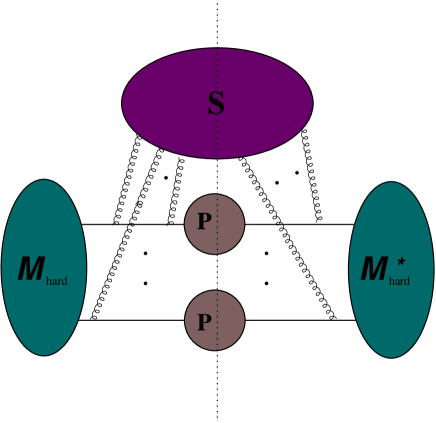
Figure 1: General structure of infrared factorization at any perturbative order. (From Ref. [18] with permission of S. Catani.)

The analytic expression for the soft factorization of the QCD matrix elements can be derived using the soft-gluon insertion technique [2, 18]. To describe this technique, we use the colour-state notation [8] for the amplitudes and the operator notation [16] for taking the soft limit of the amplitude. In the colour-state notation the amplitude for $n$ external partons is represented by the ket vector $|{\mathcal{}M}_{n}(p_{1},\dots,p_{n})\rangle$. In the limit, when momentum $p_{r}^{\mu}$ becomes soft, the $m+1$ parton amplitude fulfills the following factorization formula (for the precise meaning of the operator ${\mbox{\boldmath$\mathrm{S}$}}_{r}$ and also that of the operator ${\mbox{\boldmath$\mathrm{C}$}}_{ir}$ used below, we refer to Ref. [16])

$${\mbox{\boldmath$\mathrm{S}$}}_{r}\langle c_{r}|{\mathcal{}M}_{m+1}(p_{r},\dots)\rangle=\varepsilon^{\mu}(p_{r}){\mbox{\boldmath$J$}}_{\mu}(r,\epsilon)|{\mathcal{}M}_{m}(\dots)\rangle\,,$$ (2.1)

where $c_{r}$ is the colour-index of parton $r$. Both the amplitude and the soft current $J_{r}$ can be expanded in perturbation theory,

$$|{\mathcal{}M}\rangle =|{\mathcal{}M}^{(0)}\rangle+|{\mathcal{}M}^{(1)}\rangle+\dots\,,$$ (2.2)

$${\mbox{\boldmath$J$}}_{\alpha}(r,\epsilon) =g_{\mathrm{s}}\mu^{\epsilon}\Big{[}{\mbox{\boldmath$J$}}_{\alpha}^{(0)}(r)+(g_{\mathrm{s}}\mu^{\epsilon})^{2}{\mbox{\boldmath$J$}}_{\alpha}^{(1)}(r)+\dots\Big{]}\;.$$ (2.3)

In this letter we concentrate on the leading terms. The leading-order contribution to the soft current is

$${\mbox{\boldmath$J$}}_{\mu}^{(0)}(r)=\sum_{k=1}^{m}{\mbox{\boldmath$T$}}_{k}^{r}\frac{p_{k\mu}}{p_{k}\!\cdot\!p_{r}}\,,$$ (2.4)

where ${\mbox{\boldmath$T$}}_{k}^{r}\equiv\langle c_{r}|T_{k}^{c_{r}}$ is the colour-charge operator of parton $k$ if the emitted gluon has colour index $c_{r}$. The amplitude is a colour-singlet state, therefore colour conservation can be expressed as

$$\sum_{k=1}^{m}{\mbox{\boldmath$T$}}_{k}^{r}|{\mathcal{}M}_{m}(p_{1},\dots,p_{m})\rangle=0\,,$$ (2.5)

which implies conserved eikonal current,

$$p_{r}^{\mu}{\mbox{\boldmath$J$}}_{\mu}^{(0)}(r)|{\mathcal{}M}_{m}(p_{1},\dots,p_{m})\rangle=\sum_{k=1}^{m}{\mbox{\boldmath$T$}}_{k}^{r}|{\mathcal{}M}_{m}(p_{1},\dots,p_{m})\rangle=0\,.$$ (2.6)

The soft limit of the squared matrix element can be obtained by squaring Eq. (2.1),

$${\mbox{\boldmath$\mathrm{S}$}}_{r}|{\mathcal{}M}_{m+1}^{(0)}{(p_{r},\dots)}|^{2}=8\pi\alpha_{\mathrm{s}}\mu^{2\epsilon}\sum_{i=1}^{m}\sum_{k=1}^{m}\sum_{\rm pol.}\varepsilon_{\mu}(p_{r})\varepsilon_{\nu}^{*}(p_{r})\frac{1}{2}{\mathcal{}S}_{ik}^{\mu\nu}(r)|{\mathcal{}M}_{m;(i,k)}^{(0)}{(\dots)}|^{2}\,,$$ (2.7)

with

$${\mathcal{}S}_{ik}^{\mu\nu}(r)=\frac{4p_{i}^{\mu}p_{k}^{\nu}}{s_{ir}s_{kr}}\,,$$ (2.8)

where $s_{ir}=2p_{i}\!\cdot\!p_{r}$ and $|{\mathcal{}{M}}_{m;\,(i,k)}^{(0)}|^{2}{}$ denotes the colour-connected squared matrix element. In evaluating the square, we use axial gauge with a light-like gauge vector $n^{\mu}$ ($n^{2}=0$) to sum over the gluon polarizations, which leads to the gluon polarization tensor $d^{\mu\nu}$:

$$d^{\mu\nu}(p_{r},n)=\sum_{\rm pol.}\varepsilon_{\mu}(p_{r})\varepsilon_{\nu}^{*}(p_{r})=-g^{\mu\nu}+\frac{p_{r}^{\mu}n^{\nu}+p_{r}^{\nu}n^{\mu}}{p_{r}\!\cdot\!n}\,.$$ (2.9)

As discussed above, in a physical gauge the collinear singularities are due to the collinear splitting of an external parton, which remains true in the soft limit. The physical picture of collinear and soft emissions suggests that the collinear part of the soft gluon emission can be singled out by the diagonal term in the double sum ($i=k$) in the soft limit of the squared amplitude. As mentioned, colour-conservation implies conserved eikonal current (see Eq. (2.6)), therefore, the gauge terms in the gluon polarization tensor do not contribute. However, if we want to separate the diagonal terms from the rest, we must keep the gauge dependent terms. A short calculation yields our new formula for the soft limit of the squared matrix element:

$${\mbox{\boldmath$\mathrm{S}$}}_{r}|{\mathcal{}M}_{m+1}^{(0)}{(p_{r},\dots)}|^{2}=-8\pi\alpha_{\mathrm{s}}\mu^{2\epsilon}\sum_{i=1}^{m} \Bigg{[}\frac{1}{2}\sum_{k\neq i}^{m}\Bigg{(}{\mathcal{}S}_{ik}(r)-\frac{2s_{in}}{s_{rn}s_{ir}}-\frac{2s_{kn}}{s_{rn}s_{kr}}\Bigg{)}|{\mathcal{}M}_{m;(i,k)}^{(0)}{(\dots)}|^{2}$$ (2.10)

$$-{\mbox{\boldmath$T$}}_{i}^{2}\frac{2}{s_{ir}}\frac{s_{in}}{s_{rn}}|{\mathcal{}M}_{m}^{(0)}{(\dots)}|^{2}\Bigg{]}\,,$$

where $s_{in}=2p_{i}\!\cdot\!n$ and ${\mathcal{}S}_{ik}(r)=g_{\mu\nu}{\mathcal{}S}_{ik}^{\mu\nu}(r)$, i.e.

$${\mathcal{}S}_{ik}(r)=\frac{2s_{ik}}{s_{ir}s_{kr}}\,.$$ (2.11)

Exploiting colour conservation, the gauge-dependent terms cancel and we obtain the well-known form of soft-gluon factorization. It is easy to check that the terms in the first line, containing the colour correlations, are finite when parton $r$ is collinear to either $i$ or $k$, while those in the second line become

$${\mbox{\boldmath$\mathrm{C}$}}_{ir}{\mbox{\boldmath$\mathrm{S}$}}_{r}|{\mathcal{}M}_{m+1}^{(0)}{(p_{r},\dots)}|^{2}=8\pi\alpha_{\mathrm{s}}\mu^{2\epsilon}\sum_{i=1}^{m}{\mbox{\boldmath$T$}}_{i}^{2}\frac{2}{s_{ir}}\frac{z_{i}}{z_{r}}|{\mathcal{}M}_{m}^{(0)}{(\dots)}|^{2}\,,$$ (2.12)

in agreement with Ref. [16]. Therefore, the soft-collinear contribution has been separated in the second line.

In order to define the soft limit in Eq. (2.10) explicitly, we have to fix the gauge vector $n^{\mu}$. The choice for the gauge vector defines the infrared subtraction scheme employed for the computation of radiative corrections because if we want to avoid the double counting of the soft-collinear contribution, we have to be able to identify exactly the same expression for the soft-collinear contribution both in the soft limit (colour-diagonal piece in Eq. (2.10)) and in the collinear limit expressed in terms of momentum fractions (like in Eq. (2.12)). The momentum fractions in the Sudakov parametrization of the collinear limit are defined only in the strict collinear limit, and in order to define subtraction terms one has to extend their definition over the whole phase space. This can be done using a reference momentum $P^{\mu}$ as

$$z_{i}=\frac{s_{iP}}{s_{(ir)P}}\,,\qquad z_{r}=\frac{s_{rP}}{s_{(ir)P}}\,,$$ (2.13)

where $s_{(ir)P}=s_{iP}+s_{rP}$ so that $z_{i}+z_{r}=1$. If one aims at setting up a subtraction scheme valid at any order in perturbation theory, $P^{\mu}$ has to be chosen such that $s_{(ir)P}$ must not vanish in any of the multiple unresolved (soft and/or collinear) regions of the phase space. In Ref. [9] $P^{\mu}$ was chosen to be the total incoming momentum $Q^{\mu}$ of the event, when $z_{i}/z_{r}=s_{iQ}/s_{rQ}$, so Eq. (2.12) reads

$${\mbox{\boldmath$\mathrm{C}$}}_{ir}{\mbox{\boldmath$\mathrm{S}$}}_{r}|{\mathcal{}M}_{m+1}^{(0)}{(p_{r},\dots)}|^{2}=8\pi\alpha_{\mathrm{s}}\mu^{2\epsilon}\sum_{i=1}^{m}{\mbox{\boldmath$T$}}_{i}^{2}\frac{2}{s_{ir}}\frac{s_{iQ}}{s_{rQ}}|{\mathcal{}M}_{m}^{(0)}{(\dots)}|^{2}\,.$$ (2.14)

This expression would be identical to the colour-diagonal piece in Eq. (2.10) if the gauge vector were chosen $n^{\mu}=Q^{\mu}$, which is not possible in light-cone gauge. We may however, choose $n^{\mu}$ as

$$n^{\mu}=a_{r}(Q^{\mu}-b_{r}p_{r}^{\mu})\,,$$ (2.15)

such that $n^{2}=0$ and $s_{rn}=s_{rQ}\equiv 2p_{r}\!\cdot\!Q$. These two requirements determine $a_{r}=1$ and $b_{r}=Q^{2}/s_{rQ}$ uniquely. This choice is equivalent to the Coulomb gauge in the center of mass frame (rest frame of $Q^{\mu}$). With this gauge vector and using colour-conservation, we can rewrite Eq. (2.10) as

$${\mbox{\boldmath$\mathrm{S}$}}_{r}|{\mathcal{}M}_{m+1}^{(0)}{(p_{r},\dots)}|^{2}=-8\pi\alpha_{\mathrm{s}}\mu^{2\epsilon}\sum_{i=1}^{m} \Bigg{[}\frac{1}{2}\sum_{k\neq i}^{m}\Bigg{(}{\mathcal{}S}_{ik}(r)-\frac{2s_{iQ}}{s_{rQ}s_{ir}}-\frac{2s_{kQ}}{s_{rQ}s_{kr}}\Bigg{)}|{\mathcal{}M}_{m;(i,k)}^{(0)}{(\dots)}|^{2}$$ (2.16)

$$-{\mbox{\boldmath$T$}}_{i}^{2}\frac{2}{s_{ir}}\frac{s_{iQ}}{s_{rQ}}|{\mathcal{}M}_{m}^{(0)}{(\dots)}|^{2}\Bigg{]}\,,$$

that is, formally we can make the simple replacement $n^{\mu}\to Q^{\mu}$. Therefore, in order to avoid double subtractions, we simply drop the colour-diagonal terms from the soft factorization formula,

$${\mbox{\boldmath$\mathrm{S}$}}_{r}|{\mathcal{}M}_{m+1}^{(0)}{(p_{r},\dots)}|^{2}\to-8\pi\alpha_{\mathrm{s}}\mu^{2\epsilon}\sum_{i=1}^{m}\frac{1}{2}\sum_{k\neq i}^{m}\Bigg{(}{\mathcal{}S}_{ik}(r)-\frac{2s_{iQ}}{s_{rQ}s_{ir}}-\frac{2s_{kQ}}{s_{rQ}s_{kr}}\Bigg{)}|{\mathcal{}M}_{m;(i,k)}^{(0)}{(\dots)}|^{2}\,.$$ (2.17)

Using this purely soft limit, the collinear limit and the phase-space factorizations of Ref. [9], we arrive at the same NLO subtraction scheme as in Ref. [9]. Thus it appears that our proposal for separating the soft and collinear limits has not brought any advantage as compared to the usual technique of subtracting both and adding back a proper soft-collinear compensation term. Note however, that the separation of the soft and collinear limits based on the colour structure makes the procedure very simple to any order in perturbation theory. Furthermore, it allows for defining helicity-dependent subtractions and consequently, Monte Carlo summation of helicities in the computation of radiative corrections to jet cross sections. We discuss these two points in turn.

3 Separation of soft and collinear singularities in multiple infrared emissions

The overlapping structure of soft and collinear divergences in multiple infrared emissions becomes very complex rapidly with increasing number of unresolved partons. Already for two unresolved partons there are triply overlapping regions. The separation of these requires very careful analysis of the various infrared limits [16] and is a rather laborous excercise. The simple rules defined in the previous section can be applied to automate this cumbersome procedure as we discuss below.

We consider first the doubly soft-collinear limit when momenta $p_{i}^{\mu}$ and $p_{r}^{\mu}$ are collinear and the gluon momentum $p_{s}^{\mu}$, $(s\neq i,r)$ is soft. The factorization formula may be written in the form [18]

$${\mbox{\boldmath$\mathrm{C}$}}\kern-2.0pt{\mbox{\boldmath$\mathrm{S}$}}_{ir;s}|{\mathcal{}M}_{m+2}^{(0)}{(p_{i},p_{r},p_{s},\ldots)}|^{2}=(8\pi\alpha_{\mathrm{s}}\mu^{2\epsilon})^{2}\frac{1}{s_{ir}}$$ (3.1)

$$\times\langle{\mathcal{}M}_{m}^{(0)}(p_{(ir)},\ldots)|\frac{1}{2}\left[{\mbox{\boldmath$J$}}_{(ir)}^{\mu{\dagger}}(s,\varepsilon)d_{\mu\nu}(p_{s},n){\mbox{\boldmath$J$}}_{(ir)}^{\nu}(s,\varepsilon)\right]\hat{P}_{f_{i}f_{r}}^{(0)}(z_{i},z_{r},k_{\perp};\varepsilon)|{\mathcal{}M}_{m}^{(0)}(p_{(ir)},\ldots)\rangle\,,$$

where the soft current ${\mbox{\boldmath$J$}}_{(ir)}^{\mu}(s,\varepsilon)$ is given by Eqs. (2.3) and (2.4) with the replacement $r\to s$. The subscript $(ir)$ serves simply to remind us that in the summation in Eq. (2.4), $k$ may take the value $(ir)$, in which case the summand is

$${\mbox{\boldmath$T$}}_{(ir)}^{s}\frac{p_{(ir)\mu}}{p_{(ir)}\!\cdot\!p_{s}}\equiv({\mbox{\boldmath$T$}}_{i}^{s}+{\mbox{\boldmath$T$}}_{r}^{s})\frac{(p_{i}+p_{r})_{\mu}}{(p_{i}+p_{r})\!\cdot\!p_{s}}\,.$$ (3.2)

Retracing the steps leading to Eq. (2.16), in particular using colour conservation to make the replacement $n^{\mu}\to Q^{\mu}$, we find

$${\mbox{\boldmath$\mathrm{C}$}}\kern-2.0pt{\mbox{\boldmath$\mathrm{S}$}}_{ir;s}|{\mathcal{}M}_{m+2}^{(0)}{(p_{i},p_{r},p_{s},\ldots)}|^{2}=-(8\pi\alpha_{\mathrm{s}}\mu^{2\epsilon})^{2}\frac{1}{s_{ir}}\Bigg{[}\sum_{j=1}^{m}\sum_{k\neq j}^{m}\frac{1}{2}\left({\mathcal{}S}_{jk}(s)-\frac{2s_{jQ}}{s_{sQ}s_{js}}-\frac{2s_{kQ}}{s_{sQ}s_{ks}}\right)$$

$$\qquad\qquad\qquad\qquad\quad\times\langle{\mathcal{}M}_{m}^{(0)}(p_{(ir)},\ldots)|\hat{P}_{f_{i}f_{r}}^{(0)}(z_{i},z_{r},k_{\perp};\varepsilon){\mbox{\boldmath$T$}}_{j}{\mbox{\boldmath$T$}}_{k}|{\mathcal{}M}_{m}^{(0)}(p_{(ir)},\ldots)\rangle$$

$$\qquad\qquad\quad-\,\sum_{j\neq(ir)}^{m}{\mbox{\boldmath$T$}}_{j}^{2}\frac{2}{s_{js}}\frac{s_{jQ}}{s_{sQ}}\langle{\mathcal{}M}_{m}^{(0)}(p_{(ir)},\ldots)|\hat{P}_{f_{i}f_{r}}^{(0)}(z_{i},z_{r},k_{\perp};\varepsilon)|{\mathcal{}M}_{m}^{(0)}(p_{(ir)},\ldots)\rangle$$

$$\qquad\qquad\quad-\,{\mbox{\boldmath$T$}}_{(ir)}^{2}\frac{2}{s_{(ir)s}}\frac{s_{(ir)Q}}{s_{sQ}}\langle{\mathcal{}M}_{m}^{(0)}(p_{(ir)},\ldots)|\hat{P}_{f_{i}f_{r}}^{(0)}(z_{i},z_{r},k_{\perp};\varepsilon)|{\mathcal{}M}_{m}^{(0)}(p_{(ir)},\ldots)\rangle\Bigg{]}\,.$$ (3.3)

It is straightfroward that the product in the first two lines is finite when $p_{s}^{\mu}$ is collinear to any other momentum that appears in the matrix elements on the right hand side, including $p_{(ir)}^{\mu}$. Furthermore, defining the momentum fractions as in Ref. [10], we see that the third and fourth lines just reproduce the double and triple collinear limits of the doubly soft-collinear factorization formula (Eqs. (4.36) and (4.32) in Ref. [16]) respectively.

Next, we discuss the case of double soft parton emission. The soft-gluon insertion rules are applicable in any order of perturbation theory [18], therefore, the soft-factorization formula for the amplitude can easily be given. For instance, for two soft partons the soft current has the expansion

$${\mbox{\boldmath$J$}}_{\alpha\beta}(r,s,\varepsilon)=(g_{\mathrm{s}}\mu^{\epsilon})^{2}\Big{[}{\mbox{\boldmath$J$}}_{\alpha\beta}^{(0)}(r,s)+(g_{\mathrm{s}}\mu^{\epsilon})^{2}{\mbox{\boldmath$J$}}_{\alpha\beta}^{(1)}(r,s)+\dots\Big{]}\,,$$ (3.4)

where the leading-order contribution in light-cone gauge is [18]

$${\mbox{\boldmath$J$}}_{gg,\mu\nu}^{(0)}(r,s) =\sum_{i}^{m}\sum_{j\neq i}^{m}{\mbox{\boldmath$T$}}_{i}^{r}\,\frac{p_{i\mu}}{p_{i}\!\cdot\!p_{r}}\,{\mbox{\boldmath$T$}}_{j}^{s}\,\frac{p_{j\nu}}{p_{j}\!\cdot\!p_{s}}$$ (3.5)

$$+\sum_{i}^{m}\left({\mbox{\boldmath$T$}}_{i}^{r}\,{\mbox{\boldmath$T$}}_{i}^{s}\,\frac{p_{i\nu}}{p_{i}\!\cdot\!p_{s}}\,\frac{p_{i\mu}}{p_{i}\!\cdot\!p_{(rs)}}+{\mbox{\boldmath$T$}}_{i}^{s}\,{\mbox{\boldmath$T$}}_{i}^{r}\,\frac{p_{i\mu}}{p_{i}\!\cdot\!p_{r}}\,\frac{p_{i\nu}}{p_{i}\!\cdot\!p_{(rs)}}\right)$$

$$+\sum_{i}^{m}[{\mbox{\boldmath$T$}}_{i}^{r},{\mbox{\boldmath$T$}}_{i}^{s}]\frac{p_{i\alpha}}{p_{i}\!\cdot\!p_{(rs)}}\,d^{\alpha\beta}(p_{(rs)},n)\frac{1}{p_{r}\!\cdot\!p_{s}}V_{\beta\mu\nu}(p_{r},p_{s})\,,$$

$${\mbox{\boldmath$J$}}_{q{\bar{q}}}^{(0)}(r,s) =\sum_{i}^{m}[{\mbox{\boldmath$T$}}_{i}^{r},{\mbox{\boldmath$T$}}_{i}^{s}]\frac{p_{i\alpha}}{p_{i}\!\cdot\!p_{(rs)}}\,d^{\alpha\beta}(p_{(rs)},n)\frac{1}{p_{r}\!\cdot\!p_{s}}\gamma_{\beta}\,.$$ (3.6)

In Eqs. (3.5) and (3.6) $p_{(rs)}^{\mu}=p_{r}^{\mu}+p_{s}^{\mu}$ and

$$V_{\beta\mu\nu}(p_{r},p_{s})=\left[\frac{1}{2}(p_{r}-p_{s})_{\beta}g_{\mu\nu}+p_{s\mu}g_{\nu\beta}-p_{r\nu}g_{\mu\beta}\right]\,.$$ (3.7)

In order to separate the soft and collinear terms, we apply the same procedure as in the case of single unresolved emission, which means taking the square of the soft current and separating the colour-diagonal terms. In the case of soft-$q{\bar{q}}$ emission the algebra is relatively simple. Using $({\mbox{\boldmath$T$}}_{i}\!\cdot\!{\mbox{\boldmath$T$}}_{r})^{\dagger}({\mbox{\boldmath$T$}}_{k}\!\cdot\!{\mbox{\boldmath$T$}}_{r})=T_{\mathrm{R}}\,{\mbox{\boldmath$T$}}_{i}\!\cdot\!{\mbox{\boldmath$T$}}_{k}$, we obtain

$${\mbox{\boldmath$J$}}_{q{\bar{q}}}^{(0)\,{\dagger}}(r,s)p\kern-5.0pt/_{r}p\kern-5.0pt/_{s}{\mbox{\boldmath$J$}}_{q{\bar{q}}}^{(0)}(r,s)=\sum_{i}^{m}\sum_{k}^{m}{\mbox{\boldmath$T$}}_{i}\!\cdot\!{\mbox{\boldmath$T$}}_{k}\,\frac{p_{i}^{\mu}\,d_{\mu\alpha}(p_{(rs)},n)}{p_{i}\!\cdot\!p_{(rs)}}\,\Pi_{q{\bar{q}}}^{\alpha\beta}(p_{r},p_{s})\,\frac{d_{\beta\nu}(p_{(rs)},n)\,p_{k}^{\nu}}{p_{k}\!\cdot\!p_{(rs)}}\,,$$ (3.8)

where $\Pi_{q{\bar{q}}}^{\alpha\beta}(p_{r},p_{s})$ is the quark contribution to the discontinuity of the gluon propagator,

$$\Pi_{q{\bar{q}}}^{\alpha\beta}(p_{r},p_{s})=\frac{T_{\mathrm{R}}}{(p_{r}\!\cdot\!p_{s})^{2}}\Big{(}p_{r}^{\alpha}p_{s}^{\beta}+p_{s}^{\alpha}p_{r}^{\beta}-g^{\alpha\beta}p_{r}\!\cdot\!p_{s}\Big{)}\,.$$ (3.9)

Separating the colour-diagonal contributions we find

$${\mbox{\boldmath$J$}}_{q{\bar{q}}}^{(0)\,{\dagger}}(r,s)p\kern-5.0pt/_{r}p\kern-5.0pt/_{s}{\mbox{\boldmath$J$}}_{q{\bar{q}}}^{(0)}(r,s)=$$

$$\qquad\sum_{i}^{m}\Bigg{\{}\sum_{k\neq i}^{m}{\mbox{\boldmath$T$}}_{i}\!\cdot\!{\mbox{\boldmath$T$}}_{k}\,\frac{p_{i}^{\mu}\,d_{\mu\alpha}(p_{(rs)},n)}{p_{i}\!\cdot\!p_{(rs)}}\,\Pi_{q{\bar{q}}}^{\alpha\beta}(p_{r},p_{s})\,\frac{d_{\beta\nu}(p_{(rs)},n)\,p_{k}^{\nu}}{p_{k}\!\cdot\!p_{(rs)}}$$

$$\qquad\qquad+4\,{\mbox{\boldmath$T$}}_{i}^{2}\,T_{\mathrm{R}}\,\frac{2}{s_{i(rs)}s_{rs}}\left[\frac{s_{in}}{s_{(rs)n}}-\frac{(s_{ir}s_{sn}-s_{is}s_{rn})^{2}}{s_{i(rs)}s_{rs}s_{(rs)n}^{2}}\right]\Bigg{\}}\,.$$ (3.10)

It is now straighforward to check that in the limit when the momenta $p_{r}^{\mu}$, $p_{s}^{\mu}$ and either $p_{i}^{\mu}$ or $p_{k}^{\mu}$ are collinear, the first line in Eq. (3.10) does not contain leading collinear singularities, while the expression in the second line becomes

$${\mbox{\boldmath$\mathrm{C}$}}_{irs}{\mbox{\boldmath$J$}}_{q{\bar{q}}}^{(0)\,{\dagger}}(r,s)p\kern-5.0pt/_{r}p\kern-5.0pt/_{s}{\mbox{\boldmath$J$}}_{q{\bar{q}}}^{(0)}(r,s)=\sum_{i}^{m}4\,{\mbox{\boldmath$T$}}_{i}^{2}\,T_{\mathrm{R}}\,\frac{2}{s_{i(rs)}s_{rs}}\left[\frac{z_{i}}{z_{r}+z_{s}}-\frac{(s_{ir}z_{s}-s_{is}z_{r})^{2}}{s_{i(rs)}s_{rs}(z_{r}+z_{s})^{2}}\right]\,,$$ (3.11)

which agrees with the expression in Eq. (4.37) of Ref. [16].

We choose the gauge vector similarly as in Eq. (2.15),

$$n^{\mu}=a_{rs}(Q^{\mu}-c_{r}p_{r}^{\mu}-c_{s}p_{s}^{\mu})\,.$$ (3.12)

Requiring $n^{2}=0$, $s_{rn}=s_{rQ}$ and $s_{sn}=s_{sQ}$ (so that also $s_{(rs)n}=s_{(rs)Q}$), we can determine

$$a_{rs}=\frac{1}{R}\,,\qquad c_{r}=\frac{s_{sQ}}{s_{rs}}\,(1-R)\,,\qquad c_{s}=\frac{s_{rQ}}{s_{rs}}\,(1-R)\,,\qquad R=\sqrt{1-\frac{Q^{2}s_{rs}}{s_{rQ}s_{sQ}}}\,.$$ (3.13)

We can now use colour-conservation to see that the formal substitution $n^{\mu}\to Q^{\mu}$ can again be applied to obtain

$${\mbox{\boldmath$J$}}_{q{\bar{q}}}^{(0)\,{\dagger}}(r,s)p\kern-5.0pt/_{r}p\kern-5.0pt/_{s}{\mbox{\boldmath$J$}}_{q{\bar{q}}}^{(0)}(r,s)=\sum_{i}^{m} \Bigg{\{}\sum_{k\neq i}^{m}{\mbox{\boldmath$T$}}_{i}\!\cdot\!{\mbox{\boldmath$T$}}_{k}\,\frac{p_{i}^{\mu}\,d_{\mu\alpha}(p_{(rs)},Q)}{p_{i}\!\cdot\!p_{(rs)}}\,\Pi_{q{\bar{q}}}^{\alpha\beta}(p_{r},p_{s})\,\frac{d_{\beta\nu}(p_{(rs)},Q)\,p_{k}^{\nu}}{p_{k}\!\cdot\!p_{(rs)}}$$ (3.14)

$$+4\,{\mbox{\boldmath$T$}}_{i}^{2}\,T_{\mathrm{R}}\,\frac{2}{s_{i(rs)}s_{rs}}\left[\frac{s_{iQ}}{s_{(rs)Q}}-\frac{(s_{ir}s_{sQ}-s_{is}s_{rQ})^{2}}{s_{i(rs)}s_{rs}s_{(rs)Q}^{2}}\right]\Bigg{\}}\,.$$

The soft-collinear term is now separated in the term proportional to ${\mbox{\boldmath$T$}}_{i}^{2}$. This term can simply be dropped because it also appears in the Altarelli–Parisi splitting function of the $q\to q_{i}{\bar{q}}_{r}^{\prime}q_{s}^{\prime}$ collinear splitting [18] if the momentum fractions are defined as in Ref. [10].

The same procedure works also when two soft gluons are emitted. In this case it is more convenient to rewrite the double-current in an equivalent form in terms of colour-charge anticommutators and commutators:

$${\mbox{\boldmath$J$}}_{gg,\mu\nu}^{(0)}(r,s)=\sum_{i}^{m}\sum_{j}^{m}\frac{1}{2}\{{\mbox{\boldmath$T$}}_{i}^{r},{\mbox{\boldmath$T$}}_{j}^{s}\}\,A_{\mu\nu}^{ij}(p_{r},p_{s})+\sum_{i}^{m}[{\mbox{\boldmath$T$}}_{i}^{r},{\mbox{\boldmath$T$}}_{i}^{s}]\,C_{\mu\nu}^{i}(p_{r},p_{s})\,,$$ (3.15)

where

$$A_{\mu\nu}^{ij}(p_{r},p_{s})=\frac{p_{i\mu}}{p_{i}\!\cdot\!p_{r}}\,\frac{p_{j\nu}}{p_{j}\!\cdot\!p_{s}}$$ (3.16)

and

$$C_{\mu\nu}^{i}(p_{r},p_{s})=\frac{p_{i\alpha}d^{\alpha\beta}(p_{(rs)},n)\,V_{\beta\mu\nu}(p_{r},p_{s})}{p_{r}\!\cdot\!p_{s}\,p_{i}\!\cdot\!p_{(rs)}}-\frac{1}{2}\frac{p_{i}\!\cdot\!(p_{r}-p_{s})}{p_{i}\!\cdot\!(p_{r}+p_{s})}\frac{p_{i\mu}p_{i\nu}}{p_{i}\!\cdot\!p_{r}\,p_{i}\!\cdot\!p_{s}}\,.$$ (3.17)

In evaluating the square, we use the following colour identities:

$$\frac{1}{4}\{{\mbox{\boldmath$T$}}_{i}^{r},{\mbox{\boldmath$T$}}_{j}^{s}\}^{\dagger}\{{\mbox{\boldmath$T$}}_{k}^{r},{\mbox{\boldmath$T$}}_{l}^{s}\} =\frac{1}{2}\{{\mbox{\boldmath$T$}}_{j}\!\cdot\!{\mbox{\boldmath$T$}}_{l},{\mbox{\boldmath$T$}}_{i}\!\cdot\!{\mbox{\boldmath$T$}}_{k}\}+\frac{1}{4}C_{\mathrm{A}}\,{\mbox{\boldmath$T$}}_{i}\!\cdot\!{\mbox{\boldmath$T$}}_{k}\,\delta_{ij}\,\delta_{kl}$$ (3.18)

$$+\frac{1}{2}C_{\mathrm{A}}\Big{[}{\mbox{\boldmath$T$}}_{i}\!\cdot\!{\mbox{\boldmath$T$}}_{k}\,\delta_{il}-{\mbox{\boldmath$T$}}_{i}\!\cdot\!{\mbox{\boldmath$T$}}_{l}\,(\delta_{ik}+\delta_{kl})\Big{]}\,\delta_{jk}$$

$$+\frac{{\mathrm{i}}}{2}\>f_{abc}({\mbox{\boldmath$T$}}_{j}^{a}\,{\mbox{\boldmath$T$}}_{i}^{b}\,{\mbox{\boldmath$T$}}_{k}^{c}\,\delta_{il}-{\mbox{\boldmath$T$}}_{l}^{a}\,{\mbox{\boldmath$T$}}_{k}^{b}\,{\mbox{\boldmath$T$}}_{i}^{c}\,\delta_{jk})\,,$$

$$\frac{1}{2}\{{\mbox{\boldmath$T$}}_{i}^{r},{\mbox{\boldmath$T$}}_{j}^{s}\}^{\dagger}[{\mbox{\boldmath$T$}}_{k}^{r},{\mbox{\boldmath$T$}}_{k}^{s}] +\>\frac{1}{2}[{\mbox{\boldmath$T$}}_{k}^{r},{\mbox{\boldmath$T$}}_{k}^{s}]^{\dagger}\{{\mbox{\boldmath$T$}}_{i}^{r},{\mbox{\boldmath$T$}}_{j}^{s}\}=C_{\mathrm{A}}\,{\mbox{\boldmath$T$}}_{i}\!\cdot\!{\mbox{\boldmath$T$}}_{j}(\delta_{ik}-\delta_{jk})\,,$$ (3.19)

$$[{\mbox{\boldmath$T$}}_{i}^{r},{\mbox{\boldmath$T$}}_{i}^{s}]^{\dagger}\,[{\mbox{\boldmath$T$}}_{j}^{r},{\mbox{\boldmath$T$}}_{j}^{s}] =C_{\mathrm{A}}\,{\mbox{\boldmath$T$}}_{i}\!\cdot\!{\mbox{\boldmath$T$}}_{j}\,.$$ (3.20)

The terms proportional to the structure constants $f_{abc}$ in Eq. (3.18) are antisymmetric, while the kinematic factors that these terms multiply are symmetric when $i$ with $k$ and $j$ with $l$ are simultaneously interchanged. Therefore, these do not contribute to the square. The remaining terms contain four-fold and two-fold summations. That with four summations has single diagonal ($\sum_{i}{\mbox{\boldmath$T$}}_{i}^{2}\sum_{j}\sum_{l\neq j}{\mbox{\boldmath$T$}}_{j}\!\cdot\!{\mbox{\boldmath$T$}}_{l}$) and double diagonal ($\sum_{i}{\mbox{\boldmath$T$}}_{i}^{2}\sum_{j\neq i}{\mbox{\boldmath$T$}}_{j}^{2}$ or $\sum_{i}{\mbox{\boldmath$T$}}_{i}^{2}{\mbox{\boldmath$T$}}_{i}^{2}$) terms, which separate the soft-collinear (Eq. (4.45) in Ref. [16]), doubly-collinear (Eq. (4.43) in Ref. [16]) and abelian triply-collinear (Eq. (4.40) in Ref. [16]) contributions in the doubly-soft emissions, respectively. The contribution with two summations has single diagonal terms ($\sum_{i}{\mbox{\boldmath$T$}}_{i}^{2}$), which separate the non-abelian triply-collinear pieces (Eq. (4.41) in Ref. [16]). Again, the colour non-diagonal pieces do not have leading singularities in the various collinear limits. We choose the gauge vector as in Eq. (3.12).

4 Monte Carlo treatment of helicity summation in NLO computations

In Refs. [19, 20] a Monte Carlo integration over a phase variable for reproducing the helicity sums in the squared matrix element was introduced in order to save CPU time when computing multijet cross sections. While this approach has been found useful for computing cross sections at the LO accuracy, its extension to NLO computations is hampered by the explicit summation over the helicities in the subtraction terms used in any of the known NLO calculations. With the separation of singularities presented here, the Monte Carlo treatment of the helicity summation becomes possible by keeping the helicity states for the unresolved partons.

The Monte Carlo treatment of the helicity summation requires helicity-dependent subtraction terms. Although the soft and collinear limits of helicity amplitudes are well-known [21], the overlap between these cannot be determined at the amplitude level. In taking the square of the amplitude, keeping the helicity-dependence in the collinear subtractions is straightforward. In order to keep the helicity-dependence in the soft subtractions, one needs soft terms from which the collinear singularities are subtracted in a helicity-independent way. Our recipe does precisely that: the soft-collinear terms are identified in the colour sum. In order to define helicity-dependent soft subtractions, we do not substitute the polarization tensor $d_{\mu\nu}$ for the summations over gluon polarizations. The collinear contributions can nevertheless be separated in the colour-diagonal terms as discussed in Sect. 2.

We start from the soft factorization formula Eq. (2.7), but now we do not sum over the polarizatons of gluon $r$ or the helicities of the other $m$ partons. Separating the colour-diagonal terms as before, we have

$${\mbox{\boldmath$\mathrm{S}$}}_{r}|{\mathcal{}M}_{m+1}^{(0)}{(p_{r}^{\lambda},\dots)}|^{2}=8\pi\alpha_{\mathrm{s}}\mu^{2\epsilon}\sum_{i=1}^{m} \Bigg{[}\sum_{k\neq i}^{m}\varepsilon_{\mu}^{\lambda}(p_{r},n)\,\frac{1}{2}{\mathcal{}S}_{ik}^{\mu\nu}(r)\,\varepsilon_{\nu}^{-\lambda}(p_{r},n)|{\mathcal{}M}_{m;(i,k)}^{(0)}{(\dots)}|^{2}$$ (4.1)

$$+{\mbox{\boldmath$T$}}_{i}^{2}\,\varepsilon_{\mu}^{\lambda}(p_{r},n)\,\frac{1}{2}{\mathcal{}S}_{ii}^{\mu\nu}(r)\,\varepsilon_{\nu}^{-\lambda}(p_{r},n)|{\mathcal{}M}_{m}^{(0)}{(\dots)}|^{2}\Bigg{]}\,.\qquad~{}$$

Next, notice that the double summation over $i$ and $k$ in the first line of Eq. (4.1) effectively symmetrizes ${\mathcal{}S}^{\mu\nu}_{ik}(r)$ in its Lorentz indices, while ${\mathcal{}S}^{\mu\nu}_{ii}(r)$ in the second line is already symmetric in $\mu$ and $\nu$. Thus only the symmetric part of $\varepsilon_{\mu}^{\lambda}(p_{r},n)\varepsilon_{\nu}^{-\lambda}(p_{r},n)$ contributes. However

$$\varepsilon_{(\mu}^{\lambda}(p_{r},n)\varepsilon_{\nu)}^{-\lambda}(p_{r},n)\equiv\frac{1}{2}\left(\varepsilon_{\mu}^{\lambda}(p_{r},n)\varepsilon_{\nu}^{-\lambda}(p_{r},n)+\varepsilon_{\nu}^{\lambda}(p_{r},n)\varepsilon_{\mu}^{-\lambda}(p_{r},n)\right)=\frac{1}{2}d_{\mu\nu}(p_{r},n)\,,$$ (4.2)

and so by exactly the same steps that lead to Eq. (2.16), we obtain

$${\mbox{\boldmath$\mathrm{S}$}}_{r}|{\mathcal{}M}_{m+1}^{(0)}{(p_{r}^{\lambda},\dots)}|^{2}=-4\pi\alpha_{\mathrm{s}}\mu^{2\epsilon}\sum_{i=1}^{m} \Bigg{[}\frac{1}{2}\sum_{k\neq i}^{m}\Bigg{(}{\mathcal{}S}_{ik}(r)-\frac{2s_{iQ}}{s_{rQ}s_{ir}}-\frac{2s_{kQ}}{s_{rQ}s_{kr}}\Bigg{)}|{\mathcal{}M}_{m;(i,k)}^{(0)}{(\dots)}|^{2}$$ (4.3)

$$-{\mbox{\boldmath$T$}}_{i}^{2}\frac{2}{s_{ir}}\frac{s_{iQ}}{s_{rQ}}|{\mathcal{}M}_{m}^{(0)}{(\dots)}|^{2}\Bigg{]}\,.$$

Eq. (4.3) shows that the soft factorization formula is independent of the polarization of the emitted soft gluon. Performing the summation over the helecity $\lambda$ of the soft gluon (a multiplication by two) as well as the helicities of the rest of the partons, we trivially recover the expression in Eq. (2.16). Dropping the soft-collinear term in the second line, we find the helicity-dependent purely soft subtraction term, that clearly does not contain leading singularities when parton $r$ is collinear to either parton $i$ or parton $k$. The helicity-dependent collinear subtraction terms, including the soft-collinear contributions, can be obtained by squaring the collinear factorization formulae for helicity-amplitudes [21, 22]. Helicity-dependent subtraction terms may also be defined using the antennae factorization expressions of Refs. [23, 24].

We note that we have checked the validity of Eq. (4.3) explicitly for the processes $e^{+}e^{-}\to q{\bar{q}}g$ and $e^{+}e^{-}\to q{\bar{q}}gg$ starting from the expressions for the relevant helicity amplitudes as given in Ref. [25].

5 Summary

We have defined a new method for separating the soft and the collinear singularities in the QCD factorization formulae. The rules of the method are very simple. One starts with the soft-gluon insertion rules for finding the soft limit of the amplitudes. In taking the square of those we do not exploit colour-conservation for cancelling the gauge terms that appear in the physical polarisations of the soft gluon, rather we separate the colour-diagonal contributions. The colour non-diagonal contributions are free of leading collinear singularities, while the collinear limit of the diagonal contributions lead to the known singular expressions.

For the gauge vector $n^{\mu}$ we may choose a light-like vector whose space-like component points into opposite to that of the unresolved gluon $r$ and require that $s_{rn}=s_{rQ}$, which ensures that we can perform the formal substitution $n^{\mu}\to Q^{\mu}$, where $Q^{\mu}$ is the total four-momentum of the event. This amounts to using Coulomb gauge. We have shown that this gauge can be easily generalized to any order in perturbation theory. Choosing the momentum fractions in the collinear subtractions as in Ref. [9], the terms separated in the colour-diagonal contributions can be identified also in the collinear subtractions, therefore, can be dropped. Other choices for the gauge vectors are also possible, but we do not discuss that further in this letter.

This technique can be automatized easily and applied in any order of perturbation theory. It also facilitates the use of Monte Carlo helicity summation in the computation of the radiative corrections, therefore, can lead to significant reduction of CPU time when there are many partons in the final state, which is the most interesting case for the LHC. We should mention that a Monte Carlo treatment of colour summation also results in significant reduction of CPU time. Such treatment of colour in NLO computations is also facilitated by this new method.

Our method could be useful also for improving parton shower Monte Carlo algorithms. The algorithms that are implemented presently treat the colour correlations approximately in the large $N_{c}$ limit and sum up the leading and the next-to-leading logarithms at leading-colour accuracy. The summation of the subleading logarithms with exact colour treatment is rather difficult. However, one can go beyond the leading-colour approximation systematically by considering the subleading colour contributions pertubatively instead of exponentiating them. To do this we have to introduce subtraction terms for the subleading colour contributions in the parton shower algorithm. The technique presented here can be used to define splitting kernels and the corresponding counterterms for a parton shower algorithm since the separation of the singularities is governed by the colour structure, which provides a good control over the large logarithms and the colour structure simultaneously. We shall elaborate these ideas in separate publications.

References

• [1] G. Altarelli and G. Parisi, Nucl. Phys. B 126, 298 (1977).
• [2] A. Bassetto, M. Ciafaloni and G. Marchesini, Phys. Rept.  100, 201 (1983).
• [3] W. T. Giele and E. W. N. Glover, Annihilation,” Phys. Rev.  D 46, 1980 (1992).
• [4] W. T. Giele, E. W. N. Glover and D. A. Kosower, Nucl. Phys.  B 403, 633 (1993) [arXiv:hep-ph/9302225].
• [5] S. Frixione, Z. Kunszt and A. Signer, Nucl. Phys. B 467, 399 (1996) [arXiv:hep-ph/9512328].
• [6] Z. Nagy and Z. Trócsányi, Nucl. Phys. B 486, 189 (1997) [arXiv:hep-ph/9610498].
• [7] S. Frixione, Nucl. Phys. B 507, 295 (1997) [arXiv:hep-ph/9706545].
• [8] S. Catani and M. H. Seymour, Nucl. Phys. B 485, 291 (1997) [Erratum-ibid. B 510, 503 (1998)] [arXiv:hep-ph/9605323].
• [9] G. Somogyi and Z. Trócsányi, Acta Phys. Chim. Debr. XL, 101 (2006) [arXiv:hep-ph/0609041].
• [10] G. Somogyi, Z. Trócsányi and V. Del Duca, JHEP 0701, 070 (2007) [arXiv:hep-ph/0609042].
• [11] G. Somogyi and Z. Trócsányi, JHEP 0701, 052 (2007) [arXiv:hep-ph/0609043].
• [12] R. K. Ellis, D. A. Ross and A. E. Terrano, Nucl. Phys. B 178, 421 (1981).
• [13] J. M. Campbell, M. A. Cullen and E. W. N. Glover, Eur. Phys. J.  C 9, 245 (1999) [arXiv:hep-ph/9809429].
• [14] A. Gehrmann-De Ridder, T. Gehrmann and E. W. N. Glover, JHEP 0509, 056 (2005) [arXiv:hep-ph/0505111].
• [15] A. Daleo, T. Gehrmann and D. Maitre, arXiv:hep-ph/0612257.
• [16] G. Somogyi, Z. Trócsányi and V. Del Duca, JHEP 0506, 024 (2005) [arXiv:hep-ph/0502226].
• [17] G. Curci, W. Furmanski and R. Petronzio, Nucl. Phys.  B 175, 27 (1980).
• [18] S. Catani and M. Grazzini, Nucl. Phys. B 570, 287 (2000) [arXiv:hep-ph/9908523].
• [19] P. Draggiotis, R. H. P. Kleiss and C. G. Papadopoulos, Phys. Lett.  B 439, 157 (1998) [arXiv:hep-ph/9807207].
• [20] P. D. Draggiotis, R. H. P. Kleiss and C. G. Papadopoulos, Eur. Phys. J.  C 24, 447 (2002) [arXiv:hep-ph/0202201].
• [21] M. L. Mangano and S. J. Parke, Phys. Rept.  200, 301 (1991) [arXiv:hep-th/0509223].
• [22] T. G. Birthwright, E. W. N. Glover, V. V. Khoze and P. Marquard, JHEP 0507, 068 (2005) [arXiv:hep-ph/0505219].
• [23] D. A. Kosower, Phys. Rev.  D 57, 5410 (1998) [arXiv:hep-ph/9710213].
• [24] D. A. Kosower, Phys. Rev.  D 67, 116003 (2003) [arXiv:hep-ph/0212097].
• [25] Z. Bern, L. J. Dixon and D. A. Kosower, Nucl. Phys. B 513, 3 (1998) [arXiv:hep-ph/9708239].