Reducing the spectral index in F-term hybrid inflation through
a complementary modular inflation

Abstract

We consider two-stage inflationary models in which a superheavy scale F-term hybrid inflation is followed by an intermediate scale modular inflation. We confront these models with the restrictions on the power spectrum $P_{\cal R}$ of curvature perturbations and the spectral index $n_{\rm s}$ implied by the recent data within the power-law cosmological model with cold dark matter and a cosmological constant. We show that these restrictions can be met provided that the number of e-foldings $N_{\rm HI*}$ suffered by the pivot scale $k_{*}=0.002/{\rm Mpc}$ during hybrid inflation is appropriately restricted. The additional e-foldings required for solving the horizon and flatness problems can be naturally generated by the subsequent modular inflation. For central values of $P_{\cal R}$ and $n_{\rm s}$, we find that, in the case of standard hybrid inflation, the values obtained for the grand unification scale are close to its supersymmetric value $M_{\rm GUT}=2.86\times 10^{16}~{}{\rm GeV}$, the relevant coupling constant is relatively large ($\approx 0.005-0.14$), and $10\lesssim N_{\rm HI*}\lesssim 21.7$. In the case of shifted [smooth] hybrid inflation, the grand unification scale can be identified with $M_{\rm GUT}$ provided that $N_{\rm HI*}\simeq 21$ [$N_{\rm HI*}\simeq 18$].

1 Introduction

The recently announced three-year results wmap3 from the Wilkinson microwave anisotropy probe (WMAP3) bring under considerable stress the well-motivated, popular, and quite natural models hsusy of supersymmetric (SUSY) F-term hybrid inflation (FHI) hybrid , realized susyhybrid at (or close to) the SUSY grand unified theory (GUT) scale $M_{\rm GUT}=2.86\times 10^{16}~{}{\rm GeV}$. This is due to the fact that, in these models, the predicted spectral index $n_{\rm s}$ is too close to unity and without much running. Moreover, in the presence of non-renormalizable terms generated by supergravity (SUGRA) corrections with canonical Kähler potential, $n_{\rm s}$ approaches senoguz unity more drastically and can even exceed it. This is in conflict with the WMAP3 prediction. Indeed, fitting the WMAP3 data with the standard power-law cosmological model with cold dark matter and a cosmological constant ($\Lambda$CDM), one obtains wmap3 that, at the pivot scale $k_{*}=0.002/{\rm Mpc}$,

$$n_{\rm s}=0.958\pm 0.016~{}\Rightarrow~{}0.926\lesssim n_{\rm s}\lesssim 0.99$$ (1)

at 95$\%$ confidence level.

A way out of this inconsistency is lofti ; king based on the utilization of a quasi-canonical Kähler potential. With a convenient arrangement of the signs, a negative mass term can be induced king ; gpp in the inflationary potential of the FHI models. As a consequence, the inflationary path acquires a local maximum. Under suitable initial conditions, the so-called hilltop inflation lofti can take place as the inflaton rolls from this maximum down to smaller values. In this case, $n_{\rm s}$ can become consistent with Eq. (1), but only at the cost of an extra indispensable mild tuning gpp of the initial conditions. Alternatively, it is suggested battye that $n_{\rm s}$’s between 0.98 and 1 can be made compatible with the data by taking into account a sub-dominant contribution to the curvature perturbation due to cosmic strings, which may be (but are not necessarily trotta ) formed during the phase transition at the end of FHI. In such a case, the resulting GUT scale is constrained to values well below the SUSY GUT scale mairi ; jp ; gpp .

In this paper, we propose a two-step inflationary set-up which allows acceptable $n_{\rm s}$’s in the context of the FHI models even with canonical Kähler potential and without cosmic strings. The key point in our proposal is that the total number of e-foldings $N_{\rm tot}$ required for the resolution of the horizon and flatness problems of the standard big bang cosmology does not have to be produced exclusively during the GUT scale FHI. Since $n_{\rm s}$ within the FHI models generally decreases with the number of e-foldings $N_{\rm HI*}$ that the pivot scale $k_{*}$ suffers during FHI, we could constrain $N_{\rm HI*}$ so that Eq. (1) is satisfied. The residual number of e-foldings $N_{\rm tot}-N_{\rm HI*}$ can be obtained by a second stage of inflation realized at a lower scale. We call this type of inflation, which complements the number of e-foldings produced during the GUT scale inflation, complementary inflation. In our scenario, modular inflation (MI), which can be easily realized modular by a string axion, plays this role and produces the required additional number of e-foldings $N_{\rm tot}-N_{\rm HI*}$ with natural values of the relevant parameters. Such a construction is also beneficial for MI, since the perturbations of the inflaton in this model are not sufficiently large to account for the observations, due to its low inflationary energy scale. As an extra bonus, the gravitino constraint gravitino and the potential topological defect kibble problem of FHI can be significantly relaxed due to the enormous entropy release taking place after MI (which naturally assures a low reheat temperature). However, for the same reason, baryogenesis is made more difficult but not impossible benakli in the context of a larger scheme with (large) extra dimensions. It is interesting to note that a constrained $N_{\rm HI*}$ was previously used in Ref. yamaguchi to achieve a sufficient running of the spectral index. The additional e-foldings were provided by new inflation new .

Below, we briefly review the basic FHI models (Sec. 2) and describe the calculation of the relevant inflationary observables (Sec. 3). Then, we sketch the main features of MI (Sec. 4) and exhibit the constraints imposed on our cosmological set-up (Sec. 5). We end up with our numerical results (Sec. 6) and conclusions (Sec. 7).

2 The FHI models

The FHI can be realized hsusy adopting one of the superpotentials below:

$$W=\left\{\matrix{\kappa S\left(\bar{\Phi}\Phi-M^{2}\right)\hfill&\mbox{for standard FHI},\hfill\cr\kappa S\left(\bar{\Phi}\Phi-M^{2}\right)-S{(\bar{\Phi}\Phi)^{2}\over M_{\rm S}^{2}}\hfill&\mbox{for shifted FHI},\hfill\cr S\left({(\bar{\Phi}\Phi)^{2}\over M_{\rm S}^{2}}-\mu_{\rm S}^{2}\right)\hfill&\mbox{for smooth FHI},\hfill\cr}\right.$$ (2)

where $\bar{\Phi}$, $\Phi$ is a pair of left handed superfields belonging to non-trivial conjugate representations of a GUT gauge group $G$ and reducing its rank by their vacuum expectation values (VEVs), $S$ is a gauge singlet left handed superfield, $M_{\rm S}\sim 5\times 10^{17}~{}{\rm GeV}$ is an effective cutoff scale of the order of the string scale, and the parameters $\kappa$ and $M,~{}\mu_{\rm S}~{}(\sim M_{\rm GUT})$ are made positive by field redefinitions.

The superpotential for standard FHI in Eq. (2) is the most general renormalizable superpotential consistent with a global ${\rm U}(1)$ R symmetry susyhybrid under which

$$S\ \to\ e^{i\alpha}\,S,~{}\bar{\Phi}\Phi\ \to\ \bar{\Phi}\Phi,~{}W\to\ e^{i\alpha}\,W.$$ (3)

Including in the superpotential for standard FHI the leading non-renormalizable term, one obtains the superpotential for shifted jean FHI in Eq. (2). The superpotential for smooth pana1 FHI is produced by further imposing an extra $Z_{2}$ symmetry under which $\Phi\rightarrow-\Phi$ and, thus, allowing only even powers of the combination $\bar{\Phi}\Phi$.

From the emerging scalar potential, we can deduce that the vanishing of the D-terms implies that $|\langle\bar{\Phi}\rangle|=|\langle\Phi\rangle|$, while the vanishing of the F-terms gives the VEVs of the fields in the SUSY vacuum (in the case where $\bar{\Phi}$, $\Phi$ are not standard model (SM) singlets, $\langle\bar{\Phi}\rangle$, $\langle{\Phi}\rangle$ stand for the VEVs of their SM singlet directions). These VEVs are $\langle S\rangle=0$ and $|\langle\bar{\Phi}\rangle|=|\langle\Phi\rangle|=v_{{}_{G}}$ with

$$v_{{}_{G}}=\left\{\matrix{M\hfill&\mbox{for standard FHI},\hfill\cr\frac{M}{\sqrt{2\xi}}\sqrt{1-\sqrt{1-4\xi}}\hfill&\mbox{for shifted FHI},\hfill\cr\sqrt{\mu_{\rm S}M_{\rm S}}\hfill&\mbox{for smooth FHI},\hfill\cr}\right.$$ (4)

where $\xi=M^{2}/\kappa M_{\rm S}^{2}$ with $1/7.2<\xi<1/4$ jean . As a consequence, $W$ leads to the spontaneous breaking of $G$. The same superpotential $W$ gives also rise to hybrid inflation. This is due to the fact that, for large enough values of $|S|$, there exist flat directions i.e. valleys of local minima of the classical potential with constant (or almost constant in the case of smooth FHI) potential energy density. If we call $V_{\rm HI0}$ the dominant contribution to the (inflationary) potential energy density along these directions, we have

$$V_{\rm HI0}=\left\{\matrix{\kappa^{2}M^{4}\hfill&\mbox{for standard FHI},\hfill\cr\kappa^{2}M_{\xi}^{4}\hfill&\mbox{for shifted FHI},\hfill\cr\mu_{\rm S}^{4}\hfill&\mbox{for smooth FHI},\hfill\cr}\right.$$ (5)

with $M_{\xi}=M\sqrt{1/4\xi-1}$. Inflation can be realized if a slope along the flat direction (inflationary valley) can be generated for driving the inflaton towards the vacua. In the cases of standard susyhybrid and shifted jean FHI, this slope can be generated by the SUSY breaking on this valley. Indeed, $V_{\rm HI0}>0$ breaks SUSY and gives rise to logarithmic radiative corrections to the potential originating from a mass splitting in the $\bar{\Phi}$, $\Phi$ supermultiplets. On the other hand, in the case of smooth pana1 FHI, the inflationary valley is not classically flat and, thus, there is no need of radiative corrections. Introducing the canonically normalized inflaton field $\sigma=\sqrt{2}|S|$, the relevant correction $V_{\rm HIc}$ to the inflationary potential can be written as follows:

$$V_{\rm HIc}=\left\{\matrix{{\kappa^{4}M^{4}{\sf N}\over 32\pi^{2}}\left(2\ln{\kappa^{2}xM^{2}\over Q^{2}}+(x+1)^{2}\ln(1+x^{-1})\!+\!(x-1)^{2}\ln(1-x^{-1})\right)\hfill&\mbox{for standard FHI},\hfill\cr{\kappa^{4}M_{\xi}^{4}\over 16\pi^{2}}\left(2\ln{2\kappa^{2}x_{\xi}M_{\xi}^{2}\over Q^{2}}+(x_{\xi}+1)^{2}\ln(1+x_{\xi}^{-1})\!+\!(x_{\xi}-1)^{2}\ln(1-x_{\xi}^{-1})\right)\hfill&\mbox{for shifted FHI,}\hfill\cr-2\mu_{\rm S}^{6}M_{\rm S}^{2}/27\sigma^{4}\hfill&\mbox{for smooth FHI},\hfill\cr}\right.$$ (6)

where ${\sf N}$ is the dimensionality of the representations to which $\bar{\Phi}$ and $\Phi$ belong in the case of standard FHI, $Q$ is a renormalization scale, $x=|S|^{2}/M^{2}$, and $x_{\xi}=\sigma^{2}/M^{2}_{\xi}$. Although in our work rather large $\kappa$’s are used in the cases of standard and shifted FHI, renormalization group effects espinoza remain negligible.

For minimal Kähler potential, the leading SUGRA correction $V_{\rm HIS}$ to the scalar potential along the inflationary valley reads hybrid ; senoguz ; jp

$$V_{\rm HIS}=V_{\rm HI0}{\sigma^{4}\over 8m^{4}_{\rm P}},$$ (7)

where $m_{\rm P}\simeq 2.44\times 10^{18}~{}{\rm GeV}$ is the reduced Planck scale.

Let us also note that the most important contribution sstad to the inflationary potential from the soft SUSY breaking terms starts sstad ; jp playing an important role, in the case of standard FHI, for $\kappa\lesssim 5\times 10^{-4}$ and so it remains negligibly small in our set-up due to the large $\kappa$’s encountered (see Sec. 6). This contribution, in general, does not have sstad a significant effect in the cases of shifted and smooth FHI too.

All in all, the general form of the potential which drives the various versions of FHI reads

$$V_{\rm HI}=V_{\rm HI0}+V_{\rm HIc}+V_{\rm HIS}.$$ (8)

It is worth mentioning that the crucial difference between the standard and the other two realizations of FHI is that, during standard FHI, both $\bar{\Phi}$ and $\Phi$ vanish and so the GUT gauge group $G$ is restored. As a consequence, topological defects such as strings jp ; mairi ; gpp , monopoles, or domain walls may be produced pana1 via the Kibble mechanism kibble during the spontaneous breaking of $G$ at the end of FHI. This is avoided in the other two cases, since the form of $W$ allows the existence of non-trivial inflationary valleys along which $G$ is spontaneously broken (with the appropriate Higgs fields $\bar{\Phi}$ and $\Phi$ acquiring non-zero values). Therefore, no topological defects are produced in these cases.

3 The dynamics of FHI

Assuming (see below) that all the cosmological scales cross outside the horizon during FHI and are not reprocessed during the subsequent MI, we can apply the standard calculations (see e.g. Ref. lectures ) for the inflationary observables of FHI.

Namely, the number of e-foldings $N_{\rm HI*}$ that the pivot scale $k_{*}$ suffers during FHI can be found from

$$N_{\rm HI*}=\>\frac{1}{m^{2}_{\rm P}}\;\int_{\sigma_{\rm f}}^{\sigma_{*}}\,d\sigma\>\frac{V_{\rm HI}}{V^{\prime}_{\rm HI}},$$ (9)

where the prime denotes derivation with respect to (w.r.t.) $\sigma$, $\sigma_{*}$ is the value of $\sigma$ when the pivot scale $k_{*}$ crosses outside the horizon of FHI, and $\sigma_{\rm f}$ is the value of $\sigma$ at the end of FHI, which can be found, in the slow-roll approximation, from the condition

$$~{}~{}~{}{\sf max}\{\epsilon(\sigma_{\rm f}),|\eta(\sigma_{\rm f})|\}=1,~{}~{}\mbox{where}~{}~{}$$

$$\epsilon\simeq{m^{2}_{\rm P}\over 2}\left(\frac{V^{\prime}_{\rm HI}}{V_{\rm HI}}\right)^{2}~{}~{}\mbox{and}~{}~{}\eta\simeq m^{2}_{\rm P}~{}\frac{V^{\prime\prime}_{\rm HI}}{V_{\rm HI}}\cdot$$ (10)

In the cases of standard susyhybrid and shifted jean FHI, the end of inflation coincides with the onset of the GUT phase transition, i.e. the slow-roll conditions are violated infinitesimally close to the critical point $\sigma_{\rm c}=\sqrt{2}M$ [$\sigma_{\rm c}=M_{\xi}$] for standard [shifted] FHI, where the waterfall regime commences (this is valid even in the case where the term in Eq. (7) plays an important role). On the contrary, the end of smooth pana1 FHI is not abrupt since the inflationary path is stable w.r.t. variations in $\bar{\Phi}$, $\Phi$ for all $\sigma$’s and $\sigma_{\rm f}$ is found from Eq. (3).

The power spectrum $P_{\cal R}$ of the curvature perturbation can be calculated at the pivot scale $k_{*}$ by

$$P^{1/2}_{\cal R}=\>\frac{1}{2\sqrt{3}\,\pi m^{3}_{\rm P}}\;\left.\frac{V_{\rm HI}^{3/2}}{|V^{\prime}_{\rm HI}|}\right|_{\sigma=\sigma_{*}}\cdot$$ (11)

Finally, the spectral index $n_{\rm s}$ and its running $dn_{\rm s}/d\ln k$ are given by

$$n_{\rm s}=\>1-6\epsilon(\sigma_{*})\ +\ 2\eta(\sigma_{*})~{}~{}\mbox{and}~{}~{}~{}~{}~{}~{}~{}$$

$$dn_{\rm s}/d\ln k=\>2\left(4\eta(\sigma_{*})^{2}-(n_{\rm s}-1\right)^{2})/3-2\xi(\sigma_{*})\ ~{}~{}~{}~{}~{}$$ (12)

respectively with $\xi\simeq m_{\rm P}^{4}~{}V^{\prime}_{\rm HI}V^{\prime\prime\prime}_{\rm HI}/V^{2}_{\rm HI}$.

4 The Basics of MI

After the gravity mediated soft SUSY breaking, the potential which can support MI has the form modular

$$V_{\rm MI}=V_{\rm MI0}-\frac{1}{2}m_{s}^{2}s^{2}+\dots,$$ (13)

where the ellipsis denotes terms which are expected to stabilize $V_{\rm MI}$ at $s\sim m_{\rm P}$ with $s$ being the canonically normalized real string axion field. Therefore, in the above formula, we have

$$V_{\rm MI0}=v_{s}(m_{3/2}m_{\rm P})^{2}~{}~{}{\rm and}~{}~{}m_{s}\sim m_{3/2},$$ (14)

where $m_{3/2}\sim 1~{}{\rm TeV}$ is the gravitino mass and the coefficient $v_{s}$ is of order unity, yielding $V_{\rm MI0}^{1/4}\simeq 3\times 10^{10}~{}{\rm GeV}$. In this model, inflation can be of the fast-roll type fastroll . The field evolution is given fastroll by

$$s=s_{\rm i}e^{F_{s}\Delta N_{\rm MI}}~{}~{}{\rm with}~{}~{}F_{s}\equiv\sqrt{{9\over 4}+\left(\frac{m_{s}}{H_{s}}\right)^{2}}-{3\over 2}.$$ (15)

Here $s_{\rm i}$ is the initial value of $s$ (i.e. the value of $s$ at the onset of MI), $H_{s}\simeq\sqrt{V_{\rm MI0}}/\sqrt{3}m_{\rm P}$ is the Hubble parameter corresponding to $V_{\rm MI0}$, and $\Delta N_{\rm MI}$ is the number of e-foldings obtained from $s=s_{\rm i}$ until a given $s$.

From Eq. (15), we can estimate the total number of e-foldings during MI as

$$N_{\rm MI}\simeq\frac{1}{F_{s}}\ln\left(\frac{s_{\rm f}}{s_{\rm i}}\right),$$ (16)

where $s_{\rm f}$ is the final value of $s$. This value is given by $s_{\rm f}={\sf min}\{\langle s\rangle,s_{\rm sr}\}$, where $\langle s\rangle\sim m_{\rm P}$ is the VEV of $s$ and $s_{\rm sr}$ is determined by the condition

$$\epsilon_{\rm MI}=1~{}~{}{\rm with}~{}~{}\epsilon_{\rm MI}\equiv-\frac{\dot{H}_{\rm MI}}{H^{2}_{\rm MI}}\simeq\frac{1}{2}F_{s}^{2}\left(\frac{s}{m_{\rm P}}\right)^{2}$$ (17)

being the slow-roll parameter for MI ($H_{\rm MI}$ is the Hubble parameter during MI and the dot denotes derivation w.r.t. the cosmic time). To derive Eq. (17), we use the equation of motion for $s$ during MI and Eq. (15). For definiteness, we take $\langle s\rangle=m_{\rm P}$ in our calculation.

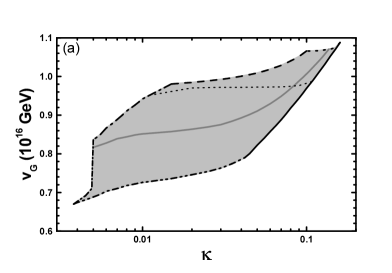
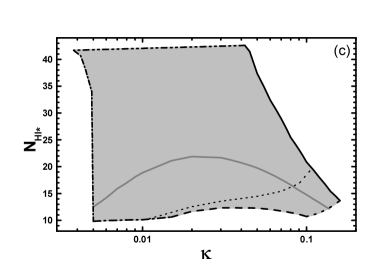
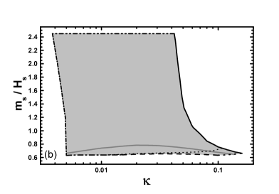
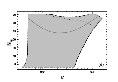
Figure 1: Allowed (lightly gray shaded) regions in the (a) $\kappa-v_{{}_{G}}$, (b) $\kappa-m_{s}/H_{s}$, (c) $\kappa-N_{\rm HI*}$, and (d) $\kappa-N_{\rm MI}$ plane for standard FHI. The black solid [dashed] lines correspond to the upper [lower] bound on $n_{\rm s}$ in Eq. (1), whereas the gray solid lines have been obtained by fixing $n_{\rm s}$ to its central value in Eq. (1). The dot-dashed [double dot-dashed] lines correspond to the lower [upper] bound on $N_{\rm HI*}~{}[m_{s}/H_{s}]$ from Eq. (21) [Eq. (23)]. The bold [faint] dotted lines correspond to $dn_{\rm s}/d\ln k=-0.01$ [$dn_{\rm s}/d\ln k=-0.005$]. Finally, the short dash-dotted lines correspond to the lower bound on $V_{\rm HI0}$ from Eq. (25). In the allowed regions, Eqs. (18) and (20) are also satisfied.

5 Observational Constraints

The cosmological scenario under consideration needs to satisfy a number of constraints. These can be outlined as follows:

• The power spectrum in Eq. (11) is to be confronted with the WMAP3 data wmap3

  $$~{}~{}~{}~{}P^{1/2}_{\cal R}\simeq\>4.86\times 10^{-5}~{}~{}\mbox{at}~{}~{}k_{*}=0.002/{\rm Mpc}.$$ (18)

• According to the inflationary paradigm, the horizon and flatness problems of the standard big bang cosmology can be successfully resolved provided that the pivot scale $k_{*}$ suffers a certain total number of e-foldings $N_{\rm tot}$, which depends on some details of the cosmological scenario. In our set-up, $N_{\rm tot}$ consists of two contributions:

  $$N_{\rm tot}=\>N_{\rm HI*}+N_{\rm MI}\,.$$ (19)

  Employing standard methods hybrid ; anupam , we can easily derive, in our case, the required $N_{\rm tot}$:

  $$~{}~{}~{}~{}N_{\rm tot}\simeq 22.6+{2\over 3}\ln{V^{1/4}_{\rm HI0}\over{1~{}{\rm GeV}}}+{1\over 3}\ln{T_{\rm Mrh}\over{1~{}{\rm GeV}}},$$ (20)

  where $T_{\rm Mrh}$ is the reheat temperature after the completion of MI. Here, we have assumed that the reheat temperature after FHI is lower than $V_{\rm MI0}^{1/4}$ (as in the majority of these models senoguz ) and, therefore, the whole inter-inflationary period is matter dominated.

  

  

  

  

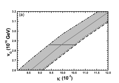
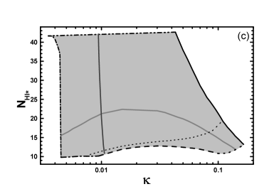
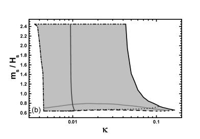
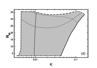
  Figure 2: Allowed regions in the (a) $\kappa-v_{{}_{G}}$, (b) $\kappa-m_{s}/H_{s}$, (c) $\kappa-N_{\rm HI*}$, and (d) $\kappa-N_{\rm MI}$ plane for shifted FHI with $M_{\rm S}=5\times 10^{17}~{}{\rm GeV}$. The notation is the same as in Fig. 1. We also include dark gray solid lines corresponding to $v_{{}_{G}}=M_{\rm GUT}$.

• We have also to assure that all the cosmological scales (i) leave the horizon during FHI and (ii) do not re-enter the horizon before the onset of MI (this would be possible since the scale factor increases faster than the horizon during the inter-inflationary era anupam ). Both these requirements can be met if we demand anupam ; astro that

  $$N_{\rm HI*}\gtrsim N^{\rm min}_{\rm HI*}\simeq 3.9+{1\over 6}\ln{V_{\rm HI0}\over V_{\rm MI0}}\cdot$$ (21)

  The first term in the expression for $N^{\rm min}_{\rm HI*}$ is the number of e-foldings elapsed between the horizon crossing of the pivot scale $k_{*}$ and the scale $0.1/{\rm Mpc}$ during FHI. Note that length scales of the order of $10~{}{\rm Mpc}$ are starting to feel nonlinear effects and it is, thus, difficult to constrain astro primordial density fluctuations on smaller scales. Given that $(V_{\rm HI0}/V_{\rm MI0})^{1/4}\sim 10^{14}/10^{10}\sim 10^{4}$, we expect that $N^{\rm min}_{\rm HI*}\sim 10$.

• As it is well known espinoza , in the models under consideration, $|dn_{\rm s}/d\ln k|$ increases as $N_{\rm HI*}$ decreases. Therefore, limiting ourselves to $|dn_{\rm s}/d\ln k|$’s consistent with the assumptions of the power-law $\Lambda$CDM cosmological model, we obtain a lower bound on $N_{\rm HI*}$. Since, within the cosmological models with running spectral index, $|dn_{\rm s}/d\ln k|$’s of order 0.01 are encountered wmap3 , we impose the following upper bound on $|dn_{\rm s}/d\ln k|$:

  $$|dn_{\rm s}/d\ln k|\ll 0.01\,.$$ (22)

  In our numerical investigation (see Sec. 6), we display boundary curves for $dn_{\rm s}/d\ln k=-0.005$ and $-0.01$.

• For MI to be natural, we constrain the dimensionless parameter $v_{s}$ in Eq. (14) as follows:

  $$~{}~{}0.5\leq v_{s}\leq 10~{}~{}\Rightarrow~{}~{}2.45\gtrsim m_{s}/H_{s}\gtrsim 0.55,$$ (23)

  where we take $m_{s}=m_{3/2}$ (see below). The lower bound on $v_{s}$ is chosen so that the sum of the two explicitly displayed terms in the right hand side of Eq. (13) is positive for $s<m_{\rm P}$. From Eq. (17), we see that, for the values of $m_{s}/H_{s}$ in Eq. (23), $s_{\rm sr}>m_{\rm P}$ and, thus, $s_{\rm f}=m_{\rm P}$. Using Eq. (16), we then find that the upper bound on $m_{s}/H_{s}$ implies the constraint $N_{\rm MI}\gtrsim 0.73\ln(m_{\rm P}/s_{\rm i})$. Note, though, that Eqs. (15)–(17) are not very accurate near the upper bound on $m_{s}/H_{s}$ since, in this region, the slow-roll parameter $\epsilon_{\rm MI}$ gets too close to unity at $s=m_{\rm P}$ and, thus, the Hubble parameter does not remain constant as $s$ approaches $m_{\rm P}$. So our results at large values of $m_{s}/H_{s}$ should be considered only as indicative. Fortunately, as we will see below, the interesting solutions are found near the lower bound on $m_{s}/H_{s}$, where the accuracy of these formulas is much better (of the order of a few per cent for $s_{\rm i}\sim 0.01\,m_{\rm P}$). Moreover, the slow-roll parameter for MI

  $$\eta_{\rm MI}\equiv m_{\rm P}^{2}\frac{V_{\rm MI}^{(2)}}{V_{\rm MI}}\simeq-\frac{1}{3}\left(\frac{m_{s}}{H_{s}}\right)^{2},$$ (24)

  where we again take $m_{s}=m_{3/2}$, satisfies the inequality $|\eta_{\rm MI}|\leq 1$ for $m_{s}/H_{s}\lesssim 1.73$ (the superscript $(n)$ denotes the $n$th derivative w.r.t. the string axion $s$). So the interesting solutions correspond to slow- rather than fast-roll MI. We should also point out that the presence of the (unspecified) terms in the ellipsis in the right hand side of Eq. (13), which are needed for stabilizing the potential at $s\sim m_{\rm P}$, also generates an uncertainty in Eqs. (15)–(17). We assume that this uncertainty is small and neglect it.

• Finally, we assume that FHI lasts long enough so that the value of the almost massless string axion $s$ is completely randomized randomize as a consequence of its quantum fluctuations from FHI. We further assume that

  $$V_{\rm MI0}\lesssim H^{4}_{\rm HI0},$$ (25)

  where $H_{\rm HI0}=\sqrt{V_{\rm HI0}}/\sqrt{3}m_{\rm P}$ is the Hubble parameter corresponding to $V_{\rm HI0}$, so that all the values of $s$ belong to the randomization region randomize . The field $s$ remains practically frozen during the inter-inflationary period since the Hubble parameter is larger than its mass. Under these circumstances, all the initial values $s_{\rm i}$ of $s$ from zero to $m_{\rm P}$ are equally probable. However, we take $s_{\rm i}\gg H_{\rm HI0}/2\pi$ so that the homogeneity of our present universe is not jeopardized by the quantum fluctuations of $s$ from FHI. Note that randomization of the value of a scalar field via inflationary quantum fluctuations requires that this field remains almost massless during inflation. For this, it is important that the field does not acquire hybrid ; effmass mass of the order of the Hubble parameter via the SUGRA scalar potential. This is, indeed, the case for the string axion during FHI (and the subsequent inter-inflationary era). In the opposite case, this field could decrease to very small values until the onset of MI as the inflaton of new inflation new in Refs. yamaguchi ; kawasaki .

6 Numerical results

In the case of standard FHI, we take ${\sf N}=2$. This corresponds to the left-right symmetric GUT gauge group ${\rm SU(3)_{c}\times SU(2)_{L}\times SU(2)_{R}\times U(1)_{B-L}}$ with $\bar{\Phi}$ and $\Phi$ belonging to ${\rm SU(2)_{R}}$ doublets with $B-L=-1$ and $1$ respectively. It is known trotta that no cosmic strings are produced during this realization of standard FHI. As a consequence, we are not obliged to impose extra restrictions on the parameters (as e.g. in Refs. mairi ; jp ). Let us mention, in passing, that, in the case of shifted jean FHI, the GUT gauge group is the Pati-Salam group ${\rm SU(4)_{c}\times SU(2)_{L}\times SU(2)_{R}}$. We take $T_{\rm Mrh}=1~{}{\rm GeV}$ and $m_{3/2}=m_{s}=1~{}{\rm TeV}$ throughout. These are indicative values which do not affect crucially our results. Indeed, $T_{\rm Mrh}$ appears in Eq. (20) through its logarithm and so its variation has a minor influence on the value of $N_{\rm tot}$. Furthermore, $N_{\rm MI}$ depends crucially only on $F_{s}$ – see Eq. (16) – which in turn depends on the ratio $m_{s}/H_{s}$ and not separately on $m_{s}$ or $H_{s}$. Finally, we choose the initial value $s_{\rm i}$ of the string axion $s$ at the onset of MI to be given by $s_{\rm i}=0.01\,m_{\rm P}$ in all the cases that we consider. This value is close enough to $m_{\rm P}$ to have a non-negligible probability to be achieved by the randomization of $s$ during FHI (see point (f) in Sec. 5). At the same time, it is adequately smaller than $m_{\rm P}$ to guarantee good accuracy of Eqs. (15)–(17) near the interesting solutions and justify the fact that we neglect the uncertainty from the terms in the ellipsis in Eq. (13) (see point (e) in Sec. 5). Moreover, larger $s_{\rm i}$’s lead to smaller parameter space for interesting solutions (with $n_{s}$ near its central value).

Table 1: Convention for the various lines in Figs. 1$-$3.

Type of Line	Corresponding Condition
Black Solid	Upper bound on $n_{\rm s}$ in Eq. (1)
Dashed	Lower bound on $n_{\rm s}$ in Eq. (1)
Short Dash-dotted	Lower bound on $V_{\rm HI0}$ from Eq. (25)
Bold Dotted	$dn_{\rm s}/d\ln k=-0.01$
Faint Dotted	$dn_{\rm s}/d\ln k=-0.005$
Dot-dashed	Lower bound on $N_{\rm HI*}$ in Eq. (21)
Double Dot-dashed	Upper bound on $m_{s}/H_{s}$ in Eq. (23)
Gray Solid	Central value of $n_{\rm s}$ in Eq. (1)
Dark Gray Solid	$v_{{}_{G}}=M_{\rm GUT}=2.86\times 10^{16}~{}{\rm GeV}$

In our numerical computation, we use, as input parameters, $\kappa$ (for standard and shifted FHI with fixed $M_{\rm S}=5\times 10^{17}~{}{\rm GeV}$) or $M_{\rm S}$ (for smooth FHI) and $\sigma_{*}$. Using Eqs. (3) and (18), we extract $n_{\rm s}$ and $v_{{}_{G}}$ respectively. For every chosen $\kappa$ or $M_{\rm S}$, we then restrict $\sigma_{*}$ so as to achieve $n_{\rm s}$ in the range of Eq. (1) and take the output values of $N_{\rm HI*}$ (contrary to the conventional strategy – see e.g. Refs. sstad ; jp – in which $N_{\rm HI*}\simeq 53$ is treated as a constraint and $n_{\rm s}$ is an output parameter). Finally, we find, from Eqs. (19) and (20), the required $N_{\rm MI}$ and the corresponding $v_{s}$ or $m_{s}/H_{s}$ from Eq. (16).

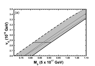
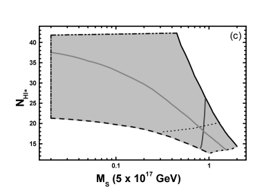
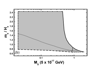
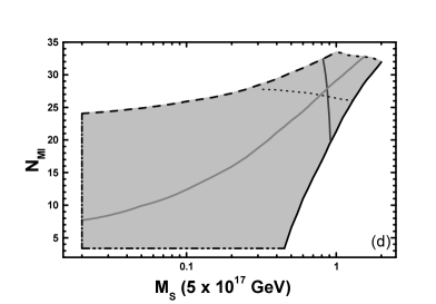
Figure 3: Allowed regions in the (a) $M_{\rm S}-v_{{}_{G}}$, (b) $M_{\rm S}-m_{s}/H_{s}$, (c) $M_{\rm S}-N_{\rm HI*}$, and (d) $M_{\rm S}-N_{\rm MI}$ plane for smooth FHI. The notation is the same as in Fig. 2. We included small $M_{\rm S}$’s of less physical interest just to show the effect of the constraints.

Our results for the three versions of FHI are presented in Figs. 1$-$3. The conventions adopted for the various lines are displayed in Table 1. In Fig. 2(a) [Fig. 3(a)], we focus on a limited range of $\kappa$’s [$M_{\rm S}$’s] for the sake of clarity of the presentation. Let us discuss each case separately:

Standard FHI.

In Fig. 1, we present the regions allowed by Eqs. (1), (18)–(23), and (25) in the (a) $\kappa-v_{{}_{G}}$, (b) $\kappa-m_{s}/H_{s}$, (c) $\kappa-N_{\rm HI*}$, and (d) $\kappa-N_{\rm MI}$ plane for standard FHI. We observe that (i) the resulting $v_{{}_{G}}$’s and $\kappa$’s are restricted to rather large values compared to those allowed within the conventional (i.e. when $N_{\rm MI}=0$) set-up (compare with Refs. sstad ; jp ), (ii) as $\kappa$ increases above 0.01 the SUGRA corrections in Eq. (7) become more and more significant, (iii) as $\kappa$ decreases below about 0.015 [0.042] the constraint from the lower [upper] bound on $n_{\rm s}$ in Eq. (1) ceases to restrict the parameters, since it is overshadowed by the lower [upper] bound on $N_{\rm HI*}$ [$m_{s}/H_{s}$] in Eq. (21) [Eq. (23)] (indeed, on the dot-dashed lines $9.84\lesssim N_{\rm HI*}=N_{\rm HI}^{\rm min}\lesssim 10.62$, which implies that $0.949\gtrsim n_{\rm s}\gtrsim 0.926$, while on the double dot-dashed ones $m_{s}/H_{s}\simeq 2.45\Rightarrow N_{\rm MI}\simeq 3.35$ yielding $n_{\rm s}\simeq 0.98-0.99$), (iv) $|dn_{\rm s}/d\ln k|$ remains well below the bound in Eq. (22) in the largest part of the regions allowed by the other constraints, whereas $-0.005\gtrsim dn_{\rm s}/d\ln k\gtrsim-0.01$ in a very limited part of these regions, and (v) for $n_{\rm s}=0.958$, we obtain $0.004\lesssim\kappa\lesssim 0.14$, $0.79\lesssim v_{{}_{G}}/(10^{16}~{}{\rm GeV})\lesssim 1.08$, and $-0.002\gtrsim dn_{\rm s}/d\ln k\gtrsim-0.01$ as well as $10\lesssim N_{\rm HI*}\lesssim 21.7$, $35\gtrsim N_{\rm MI}\gtrsim 24$, and $0.64\lesssim m_{s}/H_{s}\lesssim 0.77$.

Table 2: Input and output parameters for our scenario with shifted ($M_{\rm S}=5\times 10^{17}~{}{\rm GeV}$) or smooth FHI for $n_{\rm s}=0.958$ and $v_{{}_{G}}=M_{\rm GUT}$.

Shifted FHI			Smooth FHI
$\sigma_{*}~{}(10^{16}~{}{\rm GeV})$	$2.2$		$\sigma_{*}~{}(10^{16}~{}{\rm GeV})$	$23.53$
$\kappa$	$0.01$		$M_{\rm S}~{}(5\times 10^{17}~{}{\rm GeV})$	$0.87$
$M~{}(10^{16}~{}{\rm GeV})$	$2.35$		$\mu_{\rm S}~{}(10^{16}~{}{\rm GeV})$	$0.188$
$1/\xi$	4.54		$\sigma_{\rm f}~{}(10^{16}~{}{\rm GeV})$	$13.42$
$N_{\rm HI*}$	$21$		$N_{\rm HI*}$	$18$
$dn_{\rm s}/d\ln k$	$-0.0018$		$dn_{\rm s}/d\ln k$	$-0.0055$
$N_{\rm MI}$	$24.3$		$N_{\rm MI}$	$27.8$
$m_{s}/H_{s}$	$0.77$		$m_{s}/H_{s}$	$0.72$

Shifted FHI.

In Fig. 2, we delineate the regions allowed by Eqs. (1), (18)–(23), and (25) in the (a) $\kappa-v_{{}_{G}}$, (b) $\kappa-m_{s}/H_{s}$, (c) $\kappa-N_{\rm HI*}$, and (d) $\kappa-N_{\rm MI}$ plane for shifted FHI with $M_{\rm S}=5\times 10^{17}~{}{\rm GeV}$. We observe that (i) in contrast to the case of standard FHI, the lower [upper] bound on $N_{\rm HI*}$ [$m_{s}/H_{s}$] in Eq. (21) [Eq. (23)] gives a lower [upper] bound on $v_{{}_{G}}$ in the $\kappa-v_{{}_{G}}$ plane, (ii) the results on $m_{s}/H_{s}$, $N_{\rm HI*}$, and $N_{\rm MI}$ are quite similar to those for standard FHI (note that the bounds on $\xi$ do not cut out any slices of the allowed parameter space), and (iii) $v_{{}_{G}}$ comes out considerably larger than in the case of standard FHI and can be equal to the SUSY GUT scale (some key inputs and outputs for the interesting case $v_{{}_{G}}=M_{\rm GUT}$ with $n_{\rm s}=0.958$ are presented in Table 2).

Smooth FHI.

In Fig. 3, we present the regions allowed by Eqs. (1), (18)–(23), and (25) in the (a) $M_{\rm S}-v_{{}_{G}}$, (b) $M_{\rm S}-m_{s}/H_{s}$, (c) $M_{\rm S}-N_{\rm HI*}$, and (d) $M_{\rm S}-N_{\rm MI}$ plane for smooth FHI. We observe that (i) the SUGRA corrections in Eq. (7) play an important role for every $M_{\rm S}$ in the allowed regions of Fig. 3, (ii) in contrast to standard and shifted FHI, $|dn_{\rm s}/d\ln k|$ is considerably enhanced with $-0.005\gtrsim dn_{\rm s}/d\ln k\gtrsim-0.01$ holding in a sizable portion of the parameter space for $v_{{}_{G}}\sim M_{\rm GUT}$, (iii) the constraint of Eq. (21) does not restrict the parameters unlike the cases of standard and shifted FHI (on the dashed lines we have $0.02\lesssim M_{\rm S}/(5\times 10^{17}~{}{\rm GeV})\lesssim 1.05$, $12.6\lesssim N_{\rm HI*}\lesssim 21.3$, whereas $N^{\rm min}_{\rm HI*}\sim 10-11$), and (iv) as in the case of shifted FHI, we can find an acceptable solution fixing $n_{\rm s}=0.958$ and $v_{{}_{G}}=M_{\rm GUT}$ (some key inputs and outputs of this solution are arranged in Table 2).

7 Conclusions

We investigated a cosmological scenario tied to two bouts of inflation. The first one is a GUT scale FHI which reproduces the current data on $P_{\cal R}$ and $n_{\rm s}$ within the power-law $\Lambda$CDM cosmological model and generates a limited number of e-foldings $N_{\rm HI*}$. The second one is an intermediate scale MI which produces the residual number of e-foldings. We assume that the field which is responsible for MI is a string axion which remains naturally almost massless during FHI. We have taken into account extra restrictions on the parameters originating from (i) the resolution of the horizon and flatness problems of the standard big bang cosmology, (ii) the requirements that FHI lasts long enough to generate the observed primordial fluctuations on all the cosmological scales and that these scales are not reprocessed by the subsequent MI, (iii) the limit on the running of $n_{\rm s}$, (iv) the naturalness of MI, (v) the homogeneity of the present universe, and (vi) the complete randomization of the string axion during FHI. Fixing $n_{\rm s}$ to its central value, we concluded that (i) relatively large $\kappa$’s and $v_{{}_{G}}$’s are required within the standard FHI with $10\lesssim N_{\rm HI*}\lesssim 21.7$ and (ii) identification of the GUT breaking VEV with the SUSY GUT scale is possible within shifted [smooth] FHI with $N_{\rm HI*}\simeq 21$ [$N_{\rm HI*}\simeq 18$]. In all these cases, MI of the slow-roll type with $m_{s}/H_{s}\sim 0.6-0.8$ and a very mild tuning (of order 0.01) of the initial value of the string axion produces the necessary additional number of e-foldings. Therefore, MI complements successfully FHI.

References

- (1) D.N. Spergel et al., astro-ph/0603449.
- (2) G. Lazarides, hep-ph/0011130; R. Jeannerot, S. Khalil, and G. Lazarides, hep-ph/0106035.
- (3) E.J. Copeland, A.R. Liddle, D.H. Lyth, E.D. Stewart, and D. Wands, Phys. Rev. D 49, 6410 (1994) [astro-ph/9401011].
- (4) G.R. Dvali, Q. Shafi, and R.K. Schaefer, Phys. Rev. Lett. 73, 1886 (1994) [hep-ph/9406319]; G. Lazarides, R.K. Schaefer, and Q. Shafi, Phys. Rev. D 56, 1324 (1997) [hep-ph/9608256].
- (5) V.N. Şenoğuz and Q. Shafi, Phys. Lett. B 567, 79 (2003) [hep-ph/0305089]; ibid. 582, 6 (2003) [hep-ph/0309134].
- (6) L. Boubekeur and D. Lyth, J. Cosmol. Astropart. Phys. 07, 010 (2005) [hep-ph/0502047].
- (7) M. Bastero-Gil, S.F. King, and Q. Shafi, hep-ph/0604 198; M. ur Rehman, V.N. Şenoğuz, and Q. Shafi, Phys. Rev. D 75, 043522 (2007) [hep-ph/0612023].
- (8) B. Garbrecht, C. Pallis, and A. Pilaftsis, J. High Energy Phys. 12, 038 (2006) [hep-ph/0605264].
- (9) R.A. Battye, B. Garbrecht, and A. Moss, J. Cosmol. Astropart. Phys. 09, 007 (2006) [astro-ph/0607339].
- (10) G. Lazarides, R. Ruiz de Austri, and R. Trotta, Phys. Rev. D 70, 123527 (2005) [hep-ph/0409335].
- (11) R. Jeannerot and M. Postma, J. High Energy Phys. 05, 071 (2005) [hep-ph/0503146].
- (12) J. Rocher and M. Sakellariadou, J. Cosmol. Astropart. Phys. 03, 004 (2005) [hep-ph/0406120].
- (13) P. Binétruy and M.K. Gaillard, Phys. Rev. D 34, 3069 (1986); F.C. Adams, J.R. Bond, K. Freese, J.A. Frieman, and A.V. Olinto, ibid. 47, 426 (1993) [hep-ph/9207245]; T. Banks, M. Berkooz, S.H. Shenker, G.W. Moore, and P.J. Steinhardt, ibid. 52, 3548 (1995) [hep-th/9503114]; R. Brustein, S.P. De Alwis, and E.G. Novak, ibid. 68, 023517 (2003) [hep-th/0205042].
- (14) M.Yu. Khlopov and A.D. Linde, Phys. Lett. B 138, 265 (1984); J. Ellis, J.E. Kim, and D.V. Nanopoulos, ibid. 145, 181 (1984).
- (15) T.W.B. Kibble, J. Phys. A 9, 387 (1976).
- (16) K. Benakli and S. Davidson, Phys. Rev. D 60, 025004 (1999) [hep-ph/9810280].
- (17) M. Kawasaki, M. Yamaguchi, and J. Yokoyama, Phys. Rev. D 68, 023508 (2003) [hep-ph/0304161]; M. Yamaguchi and J. Yokoyama, ibid. 68, 123520 (2003) [hep-ph/0307373]; ibid. 70, 023513 (2004) [hep-ph/0402 282]; M. Kawasaki, T. Takayama, M. Yamaguchi, and J. Yokoyama, ibid. 74, 043525 (2006) [hep-ph/0605271].
- (18) A.D. Linde, Phys. Lett. B 108, 389 (1982); A. Albrecht and P.J. Steinhardt, Phys. Rev. Lett. 48, 1220 (1982).
- (19) R. Jeannerot, S. Khalil, G. Lazarides, and Q. Shafi, J. High Energy Phys. 10, 012 (2000) [hep-ph/0002151].
- (20) G. Lazarides and C. Panagiotakopoulos, Phys. Rev. D 52, 559 (1995) [hep-ph/9506325]; G. Lazarides, C. Panagiotakopoulos, and N.D. Vlachos, ibid. 54, 1369 (1996) [hep-ph/9606297]; R. Jeannerot, S. Khalil, and G. Laza- rides, Phys. Lett. B 506, 344 (2001) [hep-ph/0103229].
- (21) G. Ballesteros, J.A. Casas, and J.R. Espinosa, J. Cosmol. Astropart. Phys. 03, 001 (2006) [hep-ph/0601134].
- (22) V.N. Şenoğuz and Q. Shafi, Phys. Rev. D 71, 043514 (2005) [hep-ph/0412102]; hep-ph/0512170.
- (23) G. Lazarides, Lect. Notes Phys. 592, 351 (2002) [hep- ph/0111328]; J. Phys. Conf. Ser. 53, 528 (2006) [hep- ph/0607032].
- (24) A. Linde, J. High Energy Phys. 11, 052 (2001) [hep- th/0110195].
- (25) C.P. Burgess, R. Easther, A. Mazumdar, D.F. Mota, and T. Multamaki, J. High Energy Phys. 05, 067 (2005) [hep-th/0501125].
- (26) U. Seljak, A. Slosar, and P. McDonald, J. Cosmol. Astropart. Phys. 10, 014 (2006) [astro-ph/0604335].
- (27) A.A. Starobinsky and J. Yokoyama, Phys. Rev. D 50, 6357 (1994) [astro-ph/9407016]; E.J. Chun, K. Dimo- poulos, and D. Lyth, ibid. 70, 103510 (2004) [hep-ph/04 02059].
- (28) M. Dine, L. Randall, and S. Thomas, Phys. Rev. Lett. 75, 398 (1995) [hep-ph/9503303]; M.K. Gaillard, H. Murayama, and K.A. Olive, Phys. Lett. B 355, 71 (1995) [hep-ph/9504307].
- (29) K.I. Izawa, M. Kawasaki, and T. Yanagida, Phys. Lett. B 411, 249 (1997) [hep-ph/9707201]; M. Kawasaki, N. Sugiyama, and T. Yanagida, Phys. Rev. D 57, 6050 (1998) [hep-ph/9710259]; M. Kawasaki and T. Yanagida, ibid. 59, 043512 (1999) [hep-ph/9807544].