String Effects on Fermi–Dirac Correlation Measurements

Abstract:

We investigate some recent measurements of Fermi–Dirac correlations by the LEP collaborations indicating surprisingly small source radii for the production of baryons in $e^{+}e^{-}$-annihilation at the $Z^{0}$ peak. In the hadronization models there are besides the Fermi–Dirac correlation effect also a strong dynamical (anti-)correlation. We demonstrate that the extraction of the pure FD effect is highly dependent on a realistic Monte Carlo event generator, both for separation of those dynamical correlations which are not related to Fermi–Dirac statistics, and for corrections of the data and background subtractions. Although the model can be tuned to well reproduce single particle distributions, there are large model-uncertainties when it comes to correlations between identical baryons. We therefore, unfortunately, have to conclude that it is at present not possible to make any firm conclusion about the source radii relevant for baryon production at LEP.

1 Introduction

Hanbury-Brown and Twiss used Bose–Einstein (BE) correlations between photons to measure the size of distant stars [1]. A pair of bosons produced incoherently from an extended source will have an enhanced probability, $P_{12}$, to be found close in momentum space when detected simultaneously, as compared to if they are detected separately ($P_{1}$, $P_{2}$). If the production region has a Gaussian shape with some radius, $R$, it is fairly easy to show that the enhancement is given by

$$C_{\mathrm{BE}}\equiv\frac{P_{12}}{P_{1}P_{2}}=1+e^{-Q^{2}R^{2}},$$ (1)

where $Q^{2}=-(k_{1}-k_{2})^{2}$ is the negative of the square of their four-momentum difference.

It was also early proposed to use a similar analysis to gain information on the geometry of the production region for pions in high-energy collisions [2]. The assumption of completely incoherent production in a Gaussian region is obvious when considering photons from a star, and also very reasonable for the production of pions in central heavy-ion collisions. For hadronic collisions or $e^{+}e^{-}$ annihilation it may, however, seem much less natural. The assumption of incoherent production implies that the source is undisturbed by the emission, and thus not affected by the enhanced radiation. In $e^{+}e^{-}$ annihilation the source disappears in the hadronization process. Energy–momentum conservation is an important constraint, and the source is not even approximately constant. The distribution of pions is also far from isotropic, usually concentrated in narrow jets, and further complicated by the fact that the pions often come from decays of long-lived heavier resonances. In spite of all these problems, introducing a so-called caoticity parameter in eq. (1), and still assuming a Gaussian production region, all $e^{+}e^{-}$ experiments arrive at a remarkably consistent value for the size of the production region: $R\approx 0.5-1$ fm.

With a confining force, or string tension, of the order 1 GeV/fm this might have been regarded as a small production region for collisions at e.g. LEP energies where the $q\bar{q}$ pair is separated by about 90 fm before they are stopped. However, in successful models based on strings or cluster chains, hadrons which are close in momentum space originate from regions which are also close in coordinate space. Although the origin for the correlation is not fully understood, a production region for pions or kaons of the order of 1 fm is therefore quite reasonable.

An attempt to explain the observed correlation as an effect of quantum interference between different contributions to the production amplitude in the string hadronization process is presented in refs. [3, 4]. Although this approach gives a qualitatively correct result, quantitative predictions at LEP energies have been hampered by technical difficulties. Within this approach it has been argued that the correlation between string pieces separated by a gluon should be strongly reduced. When the center-of-mass energy is increased the number of gluons is also large, and the mass of a straight string piece between two gluons is kept relatively small. The result is therefore sensitive to the hadronization of small string systems. The iterative solution to the Lund string hadronization model [5] is only exact for high mass systems, and although the corrections due to finite energy normally can be neglected for inclusive distributions, they do have a large impact on correlations [6].

A natural parallel to BE correlations is to look at the corresponding correlation between identical fermions. Here one would expect a depletion of fermion pairs close in momentum space, and using the same assumptions for the production region as above we arrive at

$$C_{\mathrm{FD}}=1-\lambda e^{-Q^{2}R^{2}},$$ (2)

where we now have explicitly included the “caoticity parameter” $\lambda$. Recently three of the LEP experiments have published results on such Fermi–Dirac (FD) correlations for $pp$, $\bar{p}\bar{p}$, $\Lambda\Lambda$ and $\bar{\Lambda}\bar{\Lambda}$, again finding consistent results giving $R\sim 0.15$ fm. This result is a bit disturbing, not only because the size of the production is much smaller than the one obtained for mesons, but also because the size is smaller than the baryons themselves. It is therefore important to thoroughly investigate possible theoretical and/or experimental problems in the analyses.

An essential problem in extracting the correlation is the estimate of the reference distribution $P_{1}P_{2}$ in eq. (1). The distributions $P_{1}$ and $P_{2}$ must here correspond to exactly identical events, i.e. events with the same emission of gluon radiation (and the same orientation). If there are other correlations beside the BE or FD effect, the distribution $P_{1}P_{2}$ should be replaced by a reference distribution corresponding to the two-particle distribution in a hypothetical world without BE or FD correlations. If $N(Q)$ and $N_{\mathrm{ref}}(Q)$ represent the number of pairs in the real and the reference sample respectively, the correlation is determined by the ratio

$$C(Q)=\frac{N(Q)}{N_{\mathrm{ref}}(Q)}.$$ (3)

Such a reference sample is obviously not directly observable in an experiment. Different methods have been applied for the construction of reference samples, but they all suffer from serious limitations. One possibility is to use a phenomenological hadronization model without BE or FD correlations, implemented in a Monte Carlo event generator. Besides a strong model dependence this method is also sensitive to any imperfection in the event-generator implementation of the underlying hadronization model.

To reduce the model sensitivity it is therefore preferable to construct reference samples directly from data. Two different methods have been used for this purpose: To use opposite sign pairs and to use pairs from mixed events. When studying correlations in $\pi^{+}\pi^{+}$ or $\pi^{-}\pi^{-}$ pairs it may seem reasonable to use a reference sample of $\pi^{+}\pi^{-}$ pairs, which are free from the BE effect. The $\pi^{+}\pi^{-}$ pairs have, however, strong correlations due to resonance contributions, and when using the ratio $N_{\pi^{+}\pi^{+}}(Q^{2})/N_{\pi^{+}\pi^{-}}(Q^{2})$ to determine the BE effect, it is therefore necessary to cut out the resonance regions in the fit, or else to estimate their contributions to the distribution. The method to use a reference sample with pairs of particles from different events (a mixed reference sample) has the problem that the hadronization is dependent on the gluon radiation, which differs from event to event. This bias can be reduced (but not eliminated) by a cut in thrust, which limits the radiation, and by orienting the events to align the thrust axes.

In this paper we want to discuss the special problems encountered when trying to extract the effect of FD correlations in pairs of (anti-)protons and $\Lambda$s. Naturally there are great experimental difficulties in a determination of $\bar{p}\bar{p}$ or $\Lambda\Lambda$ correlations, which are associated with acceptance limitations, an admixture of pions in the (anti-)proton sample and limited statistics in the $\Lambda\Lambda$ sample. We will here show that the experimental analyses of momentum correlations also depend very strongly on a realistic hadronization model, which can introduce large errors due to uncertainties both in the model used and in its implementation in P YTHIA [7, 8]. We therefore conclude that it presently is not possible to confirm the very small production regions presented in the literature. It should be mentioned that there is also a model-independent method to study the FD effect, which is based on the spin correlation in $\Lambda\Lambda$ pairs. This method is, however, limited by low statistics, which also here prevents a definite conclusion.

The layout of the paper is as follows: In section 2 we describe how the experiments extract FD effects in correlations between identical baryons. Then in section 3 we present the basics of the Lund string hadronization model, where we in particular discuss baryon production and baryon–baryon correlation. In sec. 4 we discuss in more detail the uncertainties in the Lund model and the approximations in its implementation in the P YTHIA event generator, which have an impact on the baryon correlations. Finally our main results are summarized in sec. 5.

2 Measurements of Fermi–Dirac correlations

As mentioned in the introduction there are two different method, which have been used to determine the FD correlations between identical baryons. One is based on momentum correlations similar to the analyses of BE correlations between meson pairs discussed above, while the other uses spin correlations in $\Lambda\Lambda$ pairs. While the first is model dependent the second is hampered by low statistics. We will in this section discuss the results of both methods.

2.1 Momentum correlations

Experimental measurements (and theoretical expectations) show strong correlations between a proton and an anti-proton or between a $\Lambda$ and an $\bar{\Lambda}$. In the recent measurements of FD correlations between protons and $\Lambda$s, the reference samples have therefore typically been constructed using pairs of particles coming from different events, rather than opposite charge particles. To reduce the bias due to gluon radiation the events have frequently been oriented so that the thrust axes end event planes coincide, and sometimes also a lower cut on the thrust value has been applied.

Associated with the baryon–anti-baryon correlations there are in current hadronization models also very strong correlations between identical baryons, besides those caused by gluon emission. These correlations must be separated before the true FD effect can be extracted. A way to reduce the bias due to both the gluon radiation when using a mixed reference sample, and the dynamical correlations which are not due to FD statistics, is to compare with expectations from a Monte Carlo (MC) simulation program. This is usually done by studying the ”double ratio”

$$C(Q)=\left(\frac{N^{\mathrm{exp}}(Q)}{N_{\mathrm{ref}}^{\mathrm{exp}}(Q)}\right)\bigg{/}\left(\frac{N^{\mathrm{MC}}(Q)}{N_{\mathrm{ref}}^{\mathrm{MC}}(Q)}\right).$$ (4)

Here $N^{\mathrm{MC}}$ and $N_{\mathrm{ref}}^{\mathrm{MC}}$ represent the MC generated real pairs and pairs from a generated reference sample of mixed events. With a realistic MC this method should isolate the true FD effect.

We want to emphasize that this method necessarily has the problem, that the result is very sensitive to the description of the correlations in the MC, which should be free of FD effects. These correlations are much more uncertain than the inclusive distributions, which have been accurately tuned to experimental data (see e.g. [9]). Note also that they cannot be constrained by data, as it is not possible to switch off FD effects in the experiment. It is exactly the difference between the data and the FD-free MC, which is interpreted as the FD effect. If the model and/or its MC implementation is imperfect the result will be wrong. We here also note that if the MC is tuned to correctly describe the single proton spectrum, then it automatically also reproduces the pairs in the mixed events. This implies that the double ratio in eq. (4) is actually very close to the single ratio, with the MC result as the reference sample in eq. (3). As far as we know, there has been no measurements of correlations between non-identical baryons, e.g. $p\Lambda$ and $\bar{p}\bar{\Lambda}$. Such a measurement would be a very effective tool for validating the baryon–baryon correlations in the hadronization models in the absence of FD effects.

The method with double ratios has been used in analyses by the three LEP experiments ALEPH, OPAL, and DELPHI. Their results are presented in table 1, and we see that they all find similar results with a production radius of the order of 0.15 fm.

	$R\>(fm)$	$\lambda$	Experiment
$\bar{p}\bar{p}$	$0.14\pm 0.06$	$0.76\pm 0.33$	OPAL	[10]
	$0.11\pm 0.01$	$0.49\pm 0.09$	ALEPH	[11]
	$0.16\pm 0.05$	$0.67\pm 0.25$	DELPHI	[12, 13]
$\Lambda\Lambda$	$0.11\pm 0.02$	$0.59\pm 0.10$	ALEPH	[14]
	$0.17\pm 0.14$	Spin Analysis	ALEPH	[14]
	$0.19\begin{array}[c]{c}+0.37\\[-5.69054pt] -0.07\end{array}$	Spin Analysis	OPAL	[15]
	$0.11\begin{array}[c]{c}+0.05\\[-5.69054pt] -0.03\end{array}$	Spin Analysis	DELPHI	[16]

Table 1: Experimental results for $\lambda$ and $R$ from FD correlations between baryon-pairs produced in $e^{+}e^{-}$ annihilations at the LEP collider.

2.2 Spin–spin correlations

An alternative way to study the FD effect, which does not rely on theoretical models and Monte Carlo simulations, is offered by the fact that $\Lambda$ particles reveal their spin in the orientation of their decay products. A $\Lambda\Lambda$ pair with total spin 1 must have an antisymmetric spacial wave function and is therefore expected to show a suppression for small relative momenta $Q$. $\Lambda\Lambda$ pairs with total spin 0 has a symmetric spacial wave function, and should therefore show an enhancement for small $Q$, similar to the correlation for bosons. Therefore one expects pairs with small $Q$-values to be dominantly $S=0$. This ought to be revealed in a preference for the protons from the decaying $\Lambda$s to be more back to back in the di-$\Lambda$ center-of-mass system for small $Q$.

Analyses at LEP [15, 17, 14] do indicate such an effect. An example is the distribution in $dN/dy^{*}$ as obtained by the ALEPH collaboration (figure 4 in [14]). Here $y^{*}$ is the cosine of the angle between two protons in the di-$\Lambda$ center of mass system. When fitted to a straight line the resulting slope does increase for low $Q$-values, thus favouring back-to-back correlations. Results from three LEP experiments are presented in table 1, and the fitted production radii are consistent with those from analyses of momentum correlations. This type of fit to an expected form gives a very small error, but looking at the result in [14], this error cannot represent the real uncertainty in the data, which can also be well fitted by a horizontal line for all values of $Q$. Unfortunately we have to conclude that the statistics is too limited for a reliable determination of the range of the FD effect using this method. (Although in principle model independent, also this method needs Monte Carlo simulations to correct for losses due to acceptance and for background contributions.)

3 Baryon production in the Lund String Model

The most successful model of hadron production is the Lund string fragmentation model. In this model it is easy to show that two identical baryons cannot be produced close in rapidity along a jet and, hence, with small $Q$, since flavour-number conservation requires that an anti-baryon is produced in between. This need not be the case in other models. In e.g. the cluster hadronization model, two nearby clusters may both decay isotropically into baryon–anti-baryon pairs resulting in two identical baryons close in momentum space. It should be noted that although the models can be tuned to reproduce inclusive particle spectra with high accuracy, there are large uncertainties in the description of particle correlations in general and baryon correlation in particular.

As the Lund string model is used in the experimental analyses, we will here describe this model in some detail. The Lund model is based on the assumption that the colour-electric field is confined to a linear structure, analogous to a vortex line in a superconductor. The model contains two basic components: A model for the breakup of a straight force field and a model for a gluon as an excitation on the string-like field.

3.1 Breakup by $q\bar{q}$ pair production.

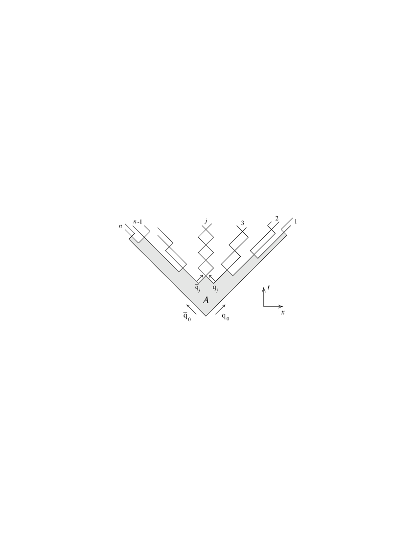
Figure 1: Schematic space–time picture of hadron production in the Lund string model.

The breakup of a high energy $q\bar{q}$ system is illustrated in fig. 1. We study first a simplified one-dimensional world with only one meson mass and no baryon production. The probability for a final state with $n$ mesons with mass $m$ and momenta $p_{i}$ is then given by the relation

$$dP\propto\prod_{i}^{n}\Bigl{[}Nd^{2}p_{i}\delta(p_{i}^{2}-m^{2})\Bigr{]}\delta\!\left(\sum p_{i}-P_{\mathrm{tot}}\right)\times\exp(-bA).$$ (5)

Here $A$ is the space-time area indicated in fig. 1, while $N$ and $b$ are two free parameters of the model. The expression in eq. (5) is a product of a phase space factor and the exponent of a ”colour coherence area”, $A$, which can be interpreted as the imaginary part of an action. The phase space is specified by the parameter $N$, where a large $N$-value favours many particles and a small $N$ few particles. The value of $b$ specifies the strength of the imaginary action, and here a large value favours early breakups and correspondingly few particles in the final mesonic state.

For a high energy system the result in eq. 5 can be generated in an iterative way. The mesons can be ”peeled off” one by one from one end, where the $i$th meson takes the fraction $z_{i}$ of the remaining (light-cone) momentum. The fractions $z_{i}$ are determined by the ”splitting function”

$$f(z)=N\frac{(1-z)^{a}}{z}\exp(-\,\frac{bm^{2}}{z}).$$ (6)

Here the parameters $N$ and $b$ are the same as in eq. (5) (if measured in units such that the string tension is 1) and $a$ is determined by the normalization constraint $\int f(z)dz=1$. (In practice, $a$ and $b$ are treated as the free parameters and $N$ is determined from normalization.)

In the real world there are different quark species and different meson masses. This is simulated by different weights $N_{i}$ in eq. (6), representing a suppression of strange quarks and of the heavier vector mesons relative to pseudo-scalar mesons. The parameter $b$ has to be a universal constant, but $a$ can in principle vary depending on the quark flavour at the breakup, although most fits to data assume a single value. It is also necessary to include transverse momenta, where the meson mass, $m$, in eqs. (5, 6) is replaced by the transverse mass $m_{\perp}=\sqrt{m^{2}+p_{\perp}^{2}}$.

We emphasized that the iterative procedure works only when the energy is large. This implies that it is a bad approximation at the end of the generation, when only little energy is remaining. In the P YTHIA program this problem is solved by peeling off mesons randomly from both ends of the string, making two hadrons when the remaining invariant mass is small enough. This implies that the error from the “junction” between the two halfs will be spread out and not visible in inclusive distributions. This method will, however, not remove the error on the correlations. They will still remain, as we will discuss further below.

3.2 Gluon emission

The second basic feature of the Lund model is the assumption that in three dimensions the dynamics of the confined force field is well represented by the massless relativistic string, and that the gluons act as transverse excitations on this string [18, 19]. This assumption implies angular asymmetries, which were first observed by the JADE collaboration at the PETRA accelerator [20]. A most important feature of this gluon model is infrared stability. Soft or collinear gluons give only small modifications of the string motion, and hence also on the final hadronic state.

Although the breakup of a string, which is bent by many gluons, should also be determined by the area law in eq. (5), there are here ambiguities and technical problems. Is the projection of a bent string piece onto a meson state the same as for a straight string piece? The generalization of eq. (5) and its formulation in an iterative process in an event generator also imply ambiguities [21]. Although an error here does not show up in inclusive distributions, it could well have effects on correlations, and thus be important in analyses of the FD effects.

3.3 Baryon production

Baryon–anti-baryon pairs can be produced when the string breaks by the production of a diquark–antidiquark pair in a $\bar{3}\!-\!3$ colour state. The weights must here be adjusted so that the baryons become fully symmetric spin-flavour states, which also preserves isospin invariance. This mechanism gives strong correlations between the baryon and the anti-baryon, which must have two quark flavours in common. This correlation is stronger than what is observed, and for this reason we have to imagine that the diquarks can be produced in a step-like manner, allowing a meson to be produced between the baryon and the anti-baryon, as indicated in fig. 2 [22]. This so called ”popcorn” mechanism also implies that the baryon and the anti-baryon come farther apart in rapidity and momentum space.

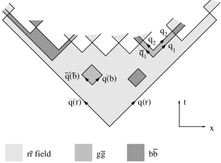
Figure 2: Representation of colour fluctuations in the string. The wrongly coloured pair $q_{1}(b)\bar{q}_{1}(\bar{b})$ together with $q_{2}(g)\bar{q}_{2}(\bar{g})$ form an effective diquark–antidiquark pair, yielding a baryon and an anti-baryon, neighbors in rank. At the left-hand side we show the production of a baryon and an anti-baryon with a meson between them, arising from two breakups in a colour fluctuation region.

A more elaborate model for baryon production is developed in ref. [23]. As we find no significant differences between this model and the standard popcorn model for the distributions of interest in this paper, we will not discuss it further here.

3.4 Baryon–anti-baryon correlations

The ordering of the hadrons along the string, the so called rank ordering, agrees on average with the ordering in rapidity, with an average separation, $\Delta y$, of the order of half a unit in rapidity. As baryon production is suppressed compared to meson production, a baryon–anti-baryon pair frequently originates from a single diquark–antidiquark breakup. The baryon and the anti-baryon are then produced as neighbours in rank, or with one (or a few) mesons in between, which implies that they are not far away from each other in momentum space. Two baryons must necessarily come from two different $B\bar{B}$ pairs, and must always be separated in rank by at least one anti-baryon (and normally also with one or more mesons). This will give a strong anti-correlation between two baryons in rapidity and in momentum. This is illustrated in fig. 3, which shows correlations in $pp$ and $p\bar{p}$ pairs. We see that there is a very strong positive correlation between protons and anti-protons, which are frequently neighbours in rank, but a negative correlation between two protons.

Figure 3: Monte Carlo results for the ratio $C_{MC}(Q)=MC(Q)/MC_{\mathrm{mix}}(Q)$ for $pp$- ($\times$) and $p\bar{p}$-pairs (+).

In fig. 3 we see that the range for the $pp$ correlation is given by $Q\sim 1.5\,\mathrm{GeV}\sim 1/(0.15\,\mathrm{fm})$. We note that this corresponds exactly to the correlation length reported in the experiments. The strength of the correlation is, however, smaller in the simulation than in the data.

This raises the question: Is the difference between data and P YTHIA really a FD effect, or could the event generator underestimate the strength of the correlation?

In the model there is a strong correlation between momentum and space coordinates for the produced hadrons. Thus two identical baryons are (in the model) well separated also in coordinate space, and we would from this picture expect Fermi–Dirac correlations to correspond to a radius $\sim 2-3$ fm. If the dynamical anti-correlation is indeed underestimated in P YTHIA , we would in the model expect that the real FD correlation corresponds to a larger radius, and therefore show up for $Q$-values around $1/(2\,\mathrm{fm})\approx 0.1\,\mathrm{GeV}$. Since the phase space is suppressed for these small $Q$-values, this effect would be impossible to observe in the LEP experiments.

Although the fundamental nature of BE correlations is not understood, its effects have been fairly well reproduced by a model in which the momenta of the produced hadrons are shifted so that identical mesons come closer in momentum space [24, 25]. This model is implemented in the program PYBOEI and included in the P YTHIA package. With minor modifications, PYBOEI can also be used to simulate FD correlations, in which case one would see an expected drop for very small $Q$-values below 0.5 GeV assuming a source radius of 1 fm.

4 Uncertainties in the event generator model

There are a number of sources for uncertainty in the P YTHIA program:

(1) There are two fundamental parameters, $a$ and $b$, in the splitting function in eq. (6). The hadron multiplicity depends essentially on the ratio $(a+1)/b$, This ratio is therefore well determined by experiments, but $a$ and $b$ separately are more uncertain. Small values of $a$ and $b$ correspond to a wide distribution $f(z)$, and a wide distribution in the separation, $\Delta y$, between hadrons which are neighbours in rank. Large values of $a$ and $b$ imply a narrow $\Delta y$-distribution and therefore lower probability for two particles to be close in momentum space. The effect of varying $a$ and $b$ keeping the multiplicity unchanged is shown in fig. 4. We see that larger $a$- and $b$-values give a stronger anti-correlation for small $Q$.

Figure 4: The ratio $C_{MC}(Q)=MC(Q)/MC_{\mathrm{mix}}(Q)$ for different values of the parameters $a$ and $b$. Larger $(a,b)$-values give a stronger correlation and a deeper dip for small $Q$. The default values in the P

YTHIA

program is $a=0.3$ and $b=0.58$ GeV^-2

Figure 5: A single jet without a junction has a large dip in $C_{MC}(Q)=MC(Q)/MC_{\mathrm{mix}}(Q)$ for small $Q$ ($\times$). This correlation is reduced by the approximate treatment in the Monte Carlo of the small mass systems close to the ”junction” (+).

Figure 6: $C_{MC}(Q)=MC(Q)/MC_{\mathrm{mix}}(Q)$ with (+) and without ($\times$) a 15% admixture of pions.

(2) The parameter $b$ is a universal constant, but $a$ may be different for baryons, although data are well fitted by a universal $a$-value. This gives some extra uncertainty.

(3) As discussed in the previous section the P YTHIA program does not exactly reproduce the Lund hadronization model. The splitting function in eq. (6) gives a correct result when the remaining energy in the system is large. To minimize the error at the end of the cascade, when the remaining invariant mass is small, the MC cuts off hadrons from both ends randomly, and joins the two ends of the system by producing two single hadrons. It is possible to adjust the cutoff so that this method works well for inclusive distributions, but it implies that the correlations do not correspond to the model prediction for particles close to the “junction”. To estimate the error from this approximation we show in fig. 5 the $pp$ correlations in a single high energy jet without a junction, and compare it with the standard result for a 91 GeV $q\bar{q}$-system. In both cases no gluon radiation is included. We note here that a significant part of the anti-correlation present in the model has disappeared in the standard Monte Carlo implementation, as the approximation in (and around) the junction allows baryons to be produced with momenta close to each other.

(4) Gluon emissions imply that straight string pieces are small compared to the mass of a $B\bar{B}B$ system. This gives also extra uncertainty. The gluon corners on the string imply ambiguities and approximations in the hadronization model [21], which even if not seen in inclusive distributions may be important for correlations. This may well be a major reason why $\pi\pi$ correlations are not so well reproduced by P YTHIA (see e.g. [26, 27]).

(5) Besides these model uncertainties, there are uncertainties in the experimental correction procedure, such as the problems with event mixing and thrust alignment mentioned in section 2. In addition the identification of anti-protons is not perfect in the experimental data. As an example the Delphi anti-proton sample contains 15% pions. As mentioned above, the pion correlations are not perfectly reproduced by P YTHIA . Fig. 6 shows results with and without a 15% pion admixture. We see that an error in the simulation of the pion–pion or pion–proton correlations also will affect the estimated proton–proton correlations.

In summary we see that there are many effects which make the Monte Carlo predictions for $pp$ or $\Lambda\Lambda$ correlations quite uncertain. As the experimental determination of the correlations rely so strongly on a correct Monte Carlo simulation, it is therfore at present premature to conclude that the production radius has the very small value around 0.15 fm. As the expected dynamical $BB$ correlation has the same range ($Q\sim 1.5\,\mathrm{GeV}$) as the published results for the FD effect, we believe that it is more likely that the strength of the dynamical $BB$ correlation is underestimated in the P YTHIA event generator. The true FD effect may then correspond to a larger production region and therefore show up at $Q$-values too small for experimental observation.

5 Conclusions

The reported results on the production radius for baryon pairs is clearly not consistent with the conventional picture of string fragmentation. In fact, a production radius of $0.15$ fm, which is smaller than the size of the baryons themselves seems difficult to reconcile with any conceivable hadronization model.

There are principal problems in the construction of a reference sample which contains all dynamical baryon–baryon correlations but not the effects of Fermi–Dirac statistics. When an event generator is tuned to inclusive distributions, the use of the double ratio in eq. (4) implies that the result depends critically on a perfect simulation program.

In this article we have noted a number of uncertainties in the Lund string fragmentation model and its implementation in the P YTHIA event generator used in the correction of the data when extracting the Fermi–Dirac effects. In particular we noted that the strong dynamical correlation between baryons in the model appears in the same range of $Q$ as the claimed FD correlations in the data, and that the model uncertainties for these correlations are large and have not been independently constrained by data.

In conclusion we feel that it is premature to claim that the observed discrepancy between data and Monte Carlo is really only due to Fermi–Dirac effects, which would indicate a new kind of production mechanism. To make such claims one would first have to demonstrate that the models correctly describe baryon–baryon correlations in the absence of FD effects, e.g. by comparing model predictions for $p\Lambda$ and $\bar{p}\bar{\Lambda}$ correlations to experimental data.

References

- [1] R. Hanbury Brown and R. Q. Twiss Nature 178 (1956) 1046–1048.
- [2] G. Goldhaber, S. Goldhaber, W.-Y. Lee, and A. Pais Phys. Rev. 120 (1960) 300–312.
- [3] B. Andersson and W. Hofmann Phys. Lett. B169 (1986) 364.
- [4] B. Andersson and M. Ringner Nucl. Phys. B513 (1998) 627–644, hep-ph/9704383.
- [5] B. Andersson, G. Gustafson, and B. Soderberg Z. Phys. C20 (1983) 317.
- [6] S. Mohanty. private communication.
- [7] T. Sjöstrand, L. Lönnblad, S. Mrenna, and P. Skands hep-ph/0308153.
- [8] T. Sjostrand, S. Mrenna, and P. Skands JHEP 05 (2006) 026, hep-ph/0603175.
- [9] K. Hamacher and M. Weierstall hep-ex/9511011.
- [10] OPAL Collaboration, “Fermi-Dirac correlations between antiprotons in hadronic Z0 decays.” OPAL note PN486, 2001.
- [11] ALEPH Collaboration, S. Schael et al. Phys. Lett. B611 (2005) 66–80.
- [12] DELPHI Collaboration, M. Kucharczyk and H. Palka, “Fermi-Dirac correlations in Z.” DELPHI note 2004-038 CONF-713, 2004.
- [13] DELPHI Collaboration, M. Kucharczyk and H. Palka, “Fermi-Dirac correlations in Z events.” DELPHI note 2005-010 CONF-730, 2004.
- [14] ALEPH Collaboration, R. Barate et al. Phys. Lett. B475 (2000) 395–406.
- [15] OPAL Collaboration, G. Alexander et al. Phys. Lett. B384 (1996) 377–387.
- [16] DELPHI Collaboration, T. Lesiak and H. Palka. Prepared for 29th International Conference on High-Energy Physics (ICHEP 98), Vancouver, British Columbia, Canada, 23-29 Jul 1998.
- [17] OPAL Collaboration, G. Abbiendi et al. Eur. Phys. J. C13 (2000) 185–195, hep-ex/9808031.
- [18] B. Andersson and G. Gustafson Zeit. Phys. C3 (1980) 223.
- [19] B. Andersson, G. Gustafson, and T. Sjostrand Zeit. Phys. C6 (1980) 235.
- [20] JADE Collaboration, W. Bartel et al. Phys. Lett. B101 (1981) 129.
- [21] T. Sjostrand Nucl. Phys. B248 (1984) 469.
- [22] B. Andersson, G. Gustafson, and T. Sjostrand Phys. Scripta 32 (1985) 574.
- [23] P. Eden and G. Gustafson Z. Phys. C75 (1997) 41–49, hep-ph/9606454.
- [24] T. Sjostrand, “Multiple Interactions, Intermittency And Other Studies,” in Multiparticle production. Proceedings, Workshop, Perugia, Italy, June 21-28, 1988, R. C. Hwa, G. Pancheri, and Y. Srivastava, eds., p. 327. 1988.
- [25] L. Lonnblad and T. Sjostrand Phys. Lett. B351 (1995) 293–301.
- [26] E. A. De Wolf. In *Santiago de Compostela 1992, Proceedings, Multiparticle dynamics* 263-274 and Brussels Interuniv. Inst. High Energy - IIHE-92-04 (92/11) 11 p. (303571) (see Conference Index).
- [27] B. Andersson, G. Gustafson, and J. Samuelsson Z. Phys. C64 (1994) 653–658.