The current problems of the minimal SO(10) GUT and their solutions

Abstract

This talk consists of two parts. In part I we review how the minimal renormalizable supersymmetric SO(10) model, an SO(10) framework with only one ${\bf 10}$ and one $\overline{\bf 126}$ Higgs multiplets in the Yukawa sector, is attractive because of its highly predictive power. Indeed it not only gives a consistent predictions on neutrino oscillation data but also gives reasonable and interesting values for leptogenesis, LFV, muon $g-2$, neutrinoless double beta decay etc. However, this model suffers from problems related to running of gauge couplings. The gauge coupling unification may be spoiled due to the presence of Higgs multiplets much lighter than the grand unification (GUT) scale. In addition, the gauge couplings blow up around the GUT scale because of the presence of Higgs multiplets of large representations. In part II we consider the minimal SO(10) model in the warped extra dimension and show a possibility to solve these problems.

1 Part I

The successful gauge coupling unification in the minimal supersymmetric standard model (MSSM), strongly supports the emergence of a supersymmetric (SUSY) GUT around $M_{\rm GUT}\simeq 2\times 10^{16}$ GeV. SO(10) is the smallest simple gauge group under which the entire SM matter content of each generation is unified into a single anomaly-free irreducible representation, ${\bf 16}$ representation. This ${\bf 16}$ representation includes right-handed neutrino and SO(10) GUT incorporates the see-saw mechanism [see-saw]. Among several models based on the gauge group SO(10), the renormalizable minimal SO(10) model has been paid a particular attention, where two Higgs multiplets $\{{\bf 10}\oplus{\bf\overline{126}}\}$ are utilized for the Yukawa couplings with matters ${\bf 16}_{i}~{}(i=\mbox{generation})$. A remarkable feature of the model is its high predictivity of the neutrino oscillation parameters as well as reproducing charged fermion masses and mixing angles.

1.1 Minimal supersymmetric SO(10) model

First we give a brief review of the renormalizable minimal SUSY SO(10) model. This model was first applied to neutrino oscillation in Ref. [Babu:1992ia]. However it did not reproduce the large mixing angles. It has been pointed out that CP-phases in the Yukawa sector play an important role to reproduce the neutrino oscillation data [Matsuda:2000zp]. More detailed analysis incorporating the renormalization group (RG) effects in the context of MSSM [Fukuyama:2002ch] has explicitly shown that the model is consistent with the neutrino oscillation data at that time and became a realistic model. We give a brief review of this renormalizable minimal SUSY SO(10) model. Yukawa coupling is given by

$$W_{Y}=Y_{10}^{ij}{\bf 16}_{i}H_{10}{\bf 16}_{j}+Y_{126}^{ij}{\bf 16}_{i}H_{126}{\bf 16}_{j}\;,$$ (1)

where ${\bf 16}_{i}$ is the matter multiplet of the $i$-th generation, $H_{10}$ and $H_{126}$ are the Higgs multiplet of 10 and $\overline{\bf 126}$ representations under SO(10), respectively. Note that, by virtue of the gauge symmetry, the Yukawa couplings, $Y_{10}$ and $Y_{126}$, are, in general, complex symmetric $3\times 3$ matrices. After the symmetry breaking pattern of SO(10) to ${\rm SU}(3)_{c}\times{\rm SU}(2)_{L}\times{\rm U}(1)_{Y}$ via ${\rm SU}(4)_{c}\times{\rm SU}(2)_{L}\times{\rm SU}(2)_{R}$ or ${\rm SU}(5)\times{\rm U}(1)$, we find two pair of Higgs doublets in the same representation as the pair in the MSSM. One pair comes from $({\bf 1},{\bf 2},{\bf 2})\subset{\bf 10}$ and the other comes from $({\bf 15},{\bf 2},{\bf 2})\subset\overline{\bf 126}$. Using these two pairs of the Higgs doublets, the Yukawa couplings of Eq. (1) are rewritten as

$$W_{Y} = (U^{c})_{i}\left(Y_{10}^{ij}H^{u}_{10}+Y_{126}^{ij}H^{u}_{126}\right)Q+(D^{c})_{i}\left(Y_{10}^{ij}H^{d}_{10}+Y_{126}^{ij}H^{d}_{126}\right)Q_{j}$$ (2)

$$+ (N^{c})_{i}\left(Y_{10}^{ij}H^{u}_{10}-3Y_{126}^{ij}H^{u}_{126}\right)L_{j}+(E^{c})_{i}\left(Y_{10}^{ij}H^{d}_{10}-3Y_{126}^{ij}H^{d}_{126}\right)L_{j}$$

$$+ L_{i}\left(Y_{126}^{ij}\;v_{T}\right)L_{j}+(N^{c})_{i}\left(Y_{126}^{ij}\;v_{R}\right)(N^{c})_{j}\;,\$$

where $U^{c}$, $D^{c}$, $N^{c}$ and $E^{c}$ are the right-handed ${\rm SU}(2)_{L}$ singlet quark and lepton superfields, $Q$ and $L$ are the left-handed ${\rm SU}(2)_{L}$ doublet quark and lepton superfields, $H_{10}^{u,d}$ and $H_{126}^{u,d}$ are up-type and down-type Higgs doublet superfields originated from $H_{10}$ and $H_{126}$, respectively, and the last term is the Majorana mass term of the right-handed neutrinos developed by the vacuum expectation value (VEV) of the $({\bf 10},{\bf 1},{\bf 3})$ Higgs, $v_{R}$. The factor $-3$ in the lepton sector is the Clebsch-Gordan (CG) coefficient.

In order to preserve the successful gauge coupling unification, suppose that one pair of Higgs doublets given by a linear combination $H_{10}^{u,d}$ and $H_{126}^{u,d}$ is light while the other pair is heavy ($\geq M_{\rm GUT}$). The light Higgs doublets are identified as the MSSM Higgs doublets ($H_{u}$ and $H_{d}$) and given by

$$H_{u} = \tilde{\alpha}_{u}H_{10}^{u}+\tilde{\beta}_{u}H_{126}^{u}\;,$$

$$H_{d} = \tilde{\alpha}_{d}H_{10}^{d}+\tilde{\beta}_{d}H_{126}^{d}\;,$$ (3)

where $\tilde{\alpha}_{u,d}$ and $\tilde{\beta}_{u,d}$ denote elements of the unitary matrix which rotate the flavor basis in the original model into the (SUSY) mass eigenstates. Omitting the heavy Higgs mass eigenstates, the low energy superpotential is described by only the light Higgs doublets $H_{u}$ and $H_{d}$ such that

$$W_{Y} = (U^{c})_{i}\left(\alpha^{u}Y_{10}^{ij}+\beta^{u}Y_{126}^{ij}\right)H_{u}\,Q_{j}+(D^{c})_{i}\left(\alpha^{d}Y_{10}^{ij}+\beta^{d}Y_{126}^{ij}\right)H_{d}\,Q_{j}$$ (4)

$$+ (N^{c})_{i}\left(\alpha^{u}Y_{10}^{ij}-3\beta^{u}Y_{126}^{ij}\right)H_{u}\,L_{j}+(E^{c})_{i}\left(\alpha^{d}Y_{10}^{ij}-3\beta^{d}Y_{126}^{ij}\right)H_{d}\,L_{j}$$

$$+ L_{i}\left(Y_{126}^{ij}\;v_{T}\right)L_{j}+(N^{c})_{i}\left(Y_{126}^{ij}v_{R}\right)(N^{c})_{j}\;,$$

where the formulas of the inverse unitary transformation of Eq. (3), $H_{10}^{u,d}=\alpha^{u,d}H_{u,d}+\cdots$ and $H_{126}^{u,d}=\beta^{u,d}H_{u,d}+\cdots$, have been used. Note that the elements of the unitary matrix, $\alpha^{u,d}$ and $\beta^{u,d}$, are in general complex parameters, through which CP-violating phases are introduced into the fermion mass matrices.

Providing the Higgs VEVs, $H_{u}=v\sin\beta$ and $H_{d}=v\cos\beta$ with $v=174\mbox{GeV}$, the quark and lepton mass matrices can be read off as

$$M_{u} = c_{10}M_{10}+c_{126}M_{126}$$

$$M_{d} = M_{10}+M_{126}$$

$$M_{D} = c_{10}M_{10}-3c_{126}M_{126}$$

$$M_{e} = M_{10}-3M_{126}$$

$$M_{T} = c_{T}M_{126}$$

$$M_{R} = c_{R}M_{126}\;,$$ (5)

where $M_{u}$, $M_{d}$, $M_{D}$, $M_{e}$, $M_{T}$, and $M_{R}$ denote the up-type quark, down-type quark, Dirac neutrino, charged-lepton, left-handed Majorana, and right-handed Majorana neutrino mass matrices, respectively. Note that all the quark and lepton mass matrices are characterized by only two basic mass matrices, $M_{10}$ and $M_{126}$, and four complex coefficients $c_{10}$, $c_{126}$, $c_{T}$ and $c_{R}$, which are defined as $M_{10}=Y_{10}\alpha^{d}v\cos\beta$, $M_{126}=Y_{126}\beta^{d}v\cos\beta$, $c_{10}=(\alpha^{u}/\alpha^{d})\tan\beta$, $c_{126}=(\beta^{u}/\beta^{d})\tan\beta$, $c_{T}=v_{T}/(\beta^{d}v\cos\beta)$) and $c_{R}=v_{R}/(\beta^{d}v\cos\beta)$), respectively. These are the mass matrix relations required by the minimal SO(10) model. In the following in Part I we set $c_{T}=0$ as the first approximation. Except for $c_{R}$, which is used to determine the overall neutrino mass scale, this system has fourteen free parameters in total [Matsuda:2000zp], which are fixed from thirteen experimental data of quarks and charged leptons leaving only one parameter $\sigma$ undetermined. (See Ref. [Fukuyama:2002ch] for the definition of $\sigma$.) Then we can fit all the neutrino oscillation data by fitting $\sigma$ and $c_{R}$. The reasonable results found in Ref. [Fukuyama:2002ch] are listed in Table 1.

The input values of $\tan\beta$, $m_{s}(M_{Z})$ and $\delta$ in the CKM matrix and the outputs for the neutrino oscillation parameters. $\tan\beta$ $m_{s}(M_{Z})$ $\delta$ $\sigma$ $\sin^{2}2\theta_{12}$ $\sin^{2}2\theta_{23}$ $\sin^{2}2\theta_{13}$ $\Delta m_{\odot}^{2}/\Delta m_{\oplus}^{2}$ 40 0.0718 $93.6^{\circ}$ 3.190 0.738 0.900 0.163 0.205 45 0.0729 $86.4^{\circ}$ 3.198 0.723 0.895 0.164 0.188 50 0.0747 $77.4^{\circ}$ 3.200 0.683 0.901 0.164 0.200 55 0.0800 $57.6^{\circ}$ 3.201 0.638 0.878 0.152 0.198

Figure 1: Three mixing angles in the MNS matrix as functions of $\sigma\mbox{[rad]}$. The graphs with the highest, middle and lowest peaks correspond to $\sin^{2}2\theta_{23}$, $\sin^{2}2\theta_{12}$ and $\sin^{2}2\theta_{13}$, respectively. The plots of $\sin^{2}2\theta_{23}$ and $\sin^{2}2\theta_{13}$ have the sharp peaks at $\sigma\sim 3.2[\mbox{rad}]$, while $\sin^{2}2\theta_{12}$ has the sharp peak at $\sigma\sim 3.3[\mbox{rad}]$ cited from Ref. [4].

As mentioned above, our resultant neutrino oscillation parameters are sensitive to all the input parameters. In other words, if we use the neutrino oscillation data as the input parameters, the other input, for example, the CP-phase in the CKM matrix can be regarded as the prediction of our model. It is a very interesting observation that the CP-phases listed above are in the region consistent with experiments. The CP-violation in the lepton sector is characterized by the Jarlskog parameter defined as

$$J_{CP}=\mbox{Im}\left[U_{e2}U_{\mu 2}^{*}U_{e3}^{*}U_{\mu 3}\right]\;,$$ (6)

where $U_{fi}$ is the MNS matrix element.

It is well known that the SO(10) GUT model possesses a simple mechanism of baryogenesis through the out-of-equilibrium decay of the right-handed neutrinos, namely, the leptogenesis [Fukugita-Yanagida]. The lepton asymmetry in the universe is generated by CP-violating out-of-equilibrium decay of the heavy neutrinos, $N\rightarrow\ell_{L}H_{u}^{*}$ and $N\rightarrow\overline{\ell_{L}}H_{u}$. The leading contribution is given by the interference between the tree level and one-loop level decay amplitudes, and the CP-violating parameter is found to be

$$\epsilon=\frac{1}{8\pi(Y_{\nu}Y_{\nu}^{\dagger})_{11}}\sum_{j=2,3}\mbox{Im}\left[(Y_{\nu}Y_{\nu}^{\dagger})_{1j}^{2}\right]\left\{f(M_{Rj}^{2}/M_{R1}^{2})+2g(M_{Rj}^{2}/M_{R1}^{2})\right\}\;.$$ (7)

Here $f(x)$ and $g(x)$ correspond to the vertex and the wave function corrections,

$$f(x) \equiv \sqrt{x}\left[1-(1+x)\mbox{ln}\left(\frac{1+x}{x}\right)\right]\;,$$

$$g(x) \equiv \frac{\sqrt{x}}{2(1-x)}\;,$$ (8)

respectively, and both are reduced to $\sim-\frac{1}{2\sqrt{x}}$ for $x\gg 1$. So in this approximation, $\epsilon$ becomes

$$\epsilon=-\frac{3}{16\pi(Y_{\nu}Y_{\nu}^{\dagger})_{11}}\sum_{j=2,3}\mbox{Im}\left[(Y_{\nu}Y_{\nu}^{\dagger})_{1j}^{2}\right]\frac{M_{R1}}{M_{Rj}}\;.$$ (9)

These quantities are evaluated by using the results presented in Table 1, and the results are listed in Table 2.

The input values of $\tan\beta$ and the outputs for the CP-violating observables $\tan\beta$ $\langle m_{\nu}\rangle_{ee}~{}(\mbox{eV})$ $J_{CP}$ $\epsilon$ 40 0.00122 $~{}~{}0.00110$ $7.39\times 10^{-5}$ 45 0.00118 $-0.00429$ $6.80\times 10^{-5}$ 50 0.00119 $-0.00631$ $6.50\times 10^{-5}$ 55 0.00117 $-0.00612$ $11.2\times 10^{-5}$

Now we turn to the discussion about the rate of the lepton flavor violating (LFV) processes and the muon $g-2$. The evidence of the neutrino flavor mixing implies that the lepton flavor of each generation is not individually conserved. Therefore the LFV processes in the charged-lepton sector such as $\mu\rightarrow e\gamma$, $\tau\rightarrow\mu\gamma$ are allowed. In simply extended models so as to incorporate massive neutrinos into the standard model, the rate of the LFV processes is accompanied by a highly suppression factor, the ratio of neutrino mass to the weak boson mass, because of the GIM mechanism, and is far out of the reach of the experimental detection. However, in supersymmetric models, the situation is quite different. In this case, soft SUSY breaking parameters can be new LFV sources, and the rate of the LFV processes are suppressed by only the scale of the soft SUSY breaking parameters which is assumed to be the electroweak scale. Thus the huge enhancement occurs compared to the previous case. In fact, the LFV processes can be one of the most important processes as the low-energy SUSY search. we evaluate the rate of the LFV processes in the minimal SUSY SO(10) model [fukuyama2], where the neutrino Dirac Yukawa couplings are the primary LFV sources. Although in Ref. [Fukuyama:2002ch] various cases with given $\tan\beta=40-55$ have been analyzed, we consider only the case $\tan\beta=45$ in the following. Our final result in the next section is almost insensitive to $\tan\beta$ values in the above range. The predictions of the minimal SUSY SO(10) model necessary for the LFV processes are as follows [Fukuyama:2002ch]: with $\sigma=3.198$ fixed, the right-handed Majorana neutrino mass eigenvalues are found to be (in GeV) $M_{R_{1}}=1.64\times 10^{11}$, $M_{R_{2}}=2.50\times 10^{12}$ and $M_{R_{3}}=8.22\times 10^{12}$, where $c_{R}$ is fixed so that $\Delta m_{\oplus}^{2}=2\times 10^{-3}\mbox{eV}^{2}$. In the basis where both of the charged-lepton and right-handed Majorana neutrino mass matrices are diagonal with real and positive eigenvalues, the neutrino Dirac Yukawa coupling matrix at the GUT scale is found to be

$$Y_{\nu}=\left(\begin{array}[]{ccc}-0.000135-0.00273i&0.00113+0.0136i&0.0339+0.0580i\\ 0.00759+0.0119i&-0.0270-0.00419i&-0.272-0.175i\\ -0.0280+0.00397i&0.0635-0.0119i&0.491-0.526i\end{array}\right)\;.$$ (13)

LFV effect most directly emerges in the left-handed slepton mass matrix through the RGEs such as [Hisano]:

$$\mu\frac{d}{d\mu}\left(m^{2}_{\tilde{\ell}}\right)_{ij} = \mu\frac{d}{d\mu}\left(m^{2}_{\tilde{\ell}}\right)_{ij}\Big{|}_{\mbox{MSSM}}$$

$$+ \frac{1}{16\pi^{2}}\left(m^{2}_{\tilde{\ell}}Y_{\nu}^{\dagger}Y_{\nu}+Y_{\nu}^{\dagger}Y_{\nu}m^{2}_{\tilde{\ell}}+2Y_{\nu}^{\dagger}m^{2}_{\tilde{\nu}}Y_{\nu}+2m_{H_{u}}^{2}Y_{\nu}^{\dagger}Y_{\nu}+2A_{\nu}^{\dagger}A_{\nu}\right)_{ij}\;,$$

where the first term in the right hand side denotes the normal MSSM term with no LFV. We have found $Y_{\nu}$ explicitly and we can calculate LFV and related phenomena unambiguously [fukuyama2] In the leading-logarithmic approximation, the off-diagonal components ($i\neq j$) of the left-handed slepton mass matrix are estimated as

$$\left(\Delta m^{2}_{\tilde{\ell}}\right)_{ij}\sim-\frac{3m_{0}^{2}+A_{0}^{2}}{8\pi^{2}}\left(Y_{\nu}^{\dagger}LY_{\nu}\right)_{ij}\;,$$ (15)

where the distinct thresholds of the right-handed Majorana neutrinos are taken into account by the matrix $L=\log[M_{\rm GUT}/M_{R_{i}}]\delta_{ij}$.

The effective Lagrangian relevant for the LFV processes ($\ell_{i}\rightarrow\ell_{j}\gamma$) and the muon $g-2$ is described as

$${\cal L}_{\mbox{eff}}=-\frac{e}{2}m_{\ell_{i}}\overline{\ell}_{j}\sigma_{\mu\nu}F^{\mu\nu}\left(A_{L}^{ji}P_{L}+A_{R}^{ji}P_{R}\right)\ell_{i}\;,$$ (16)

where $P_{R,L}=(1\pm\gamma_{5})/2$ is the chirality projection operator, and $A_{L,R}$ are the photon-penguin couplings of 1-loop diagrams in which chargino-sneutrino and neutralino-charged slepton are running. The explicit formulas of $A_{L,R}$ etc. used in our analysis are summarized in Ref. [Hisano-etal, Okada-etal]. The rate of the LFV decay of charged-leptons is given by

$$\Gamma(\ell_{i}\rightarrow\ell_{j}\gamma)=\frac{e^{2}}{16\pi}m_{\ell_{i}}^{5}\left(|A_{L}^{ji}|^{2}+|A_{R}^{ji}|^{2}\right)\;,$$ (17)

while the real diagonal components of $A_{L,R}$ contribute to the anomalous magnetic moments of the charged-leptons such as

$$\delta a_{\ell_{i}}^{\rm SUSY}=\frac{g_{\ell_{i}}-2}{2}=-m_{\ell_{i}}^{2}\mbox{Re}\left[A_{L}^{ii}+A_{R}^{ii}\right]\;.$$ (18)

In order to clarify the parameter dependence of the decay amplitude, we give here an approximate formula of the LFV decay rate [Hisano-etal],

$$\Gamma(\ell_{i}\rightarrow\ell_{j}\gamma)\sim\frac{e^{2}}{16\pi}m_{\ell_{i}}^{5}\times\frac{\alpha_{2}}{16\pi^{2}}\frac{\left|(\Delta m^{2}_{\tilde{\ell}})_{ij}\right|^{2}}{M_{S}^{8}}\tan^{2}\beta\;,$$ (19)

where $M_{S}$ is the average slepton mass at the electroweak scale, and $\left(\Delta m^{2}_{\tilde{\ell}}\right)_{ij}$ is the slepton mass estimated in Eq. (15). We can see that the neutrino Dirac Yukawa coupling matrix plays the crucial role in calculations of the LFV processes. We use the neutrino Dirac Yukawa coupling matrix of Eq. (13) in our numerical calculations.

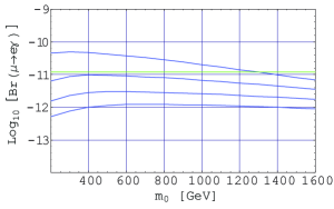
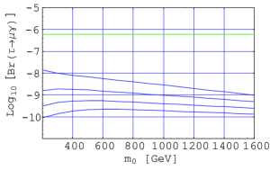
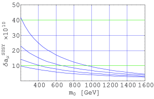
Figure 2: The branching ratios, (a) $\mbox{Log}_{10}\left[\mbox{Br}(\mu\rightarrow e\gamma)\right]$, (b) $\mbox{Log}_{10}\left[\mbox{Br}(\tau\rightarrow\mu\gamma)\right]$. and (c) the SUSY contribution to the muon $g-2$ in units of $10^{-10}$, $\delta a_{\ell_{i}}^{\rm SUSY}=\frac{g_{\ell_{i}}-2}{2}$. All these figures are plotted as a function of $m_{0}$ (GeV) for $M_{1/2}=400,600,800,1000$ GeV (from top to bottom) with $A_{0}=0$ and $\mu>0$ cited from Ref. [6].

The recent Wilkinson Microwave Anisotropy Probe (WMAP) satellite data [WMAP] provide estimations of various cosmological parameters with greater accuracy. The current density of the universe is composed of about 73% of dark energy and 27% of matter. Most of the matter density is in the form of the CDM, and its density is estimated to be (in 2$\sigma$ range)

$$\Omega_{\rm CDM}h^{2}=0.1126^{+0.0161}_{-0.0181}\;.$$ (20)

The parameter space of the CMSSM which allows the neutralino relic density suitable for the cold dark matter has been recently re-examined in the light of the WMAP data [CDM]. It has been shown that the resultant parameter space is dramatically reduced into the narrow stripe due to the great accuracy of the WMAP data. It is interesting to combine this result with our analysis of the LFV processes and the muon $g-2$. In the case relevant for our analysis, $\tan\beta=45$, $\mu>0$ and $A_{0}=0$, we can read off the approximate relation between $m_{0}$ and $M_{1/2}$ such as (see Figure 1 in the second paper of Ref. [CDM].)

$$m_{0}(\mbox{GeV})=\frac{9}{28}M_{1/2}(\mbox{GeV})+150(\mbox{GeV})\;,$$ (21)

along which the neutralino CDM is realized. $M_{1/2}$ parameter space is constrained within the range $300\mbox{GeV}\leq M_{1/2}\leq 1000\mbox{GeV}$ due to the experimental bound on the SUSY contribution to the $b\rightarrow s\gamma$ branching ratio and the unwanted stau LSP parameter region. We show $\mbox{Br}(\mu\rightarrow e\gamma)$ and the muon $g-2$ as functions of $M_{1/2}$ in Fig. 3 and 3, respectively, along the neutralino CDM condition of Eq. (21). We find the parameter region, $560\mbox{GeV}\leq M_{1/2}\leq 800\mbox{GeV}$, being consistent with all the experimental data.

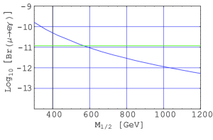
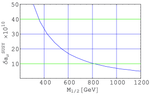
Figure 3: The branching ratio, (a) $\mbox{Log}_{10}\left[{\rm Br}(\mu\rightarrow e\gamma)\right]$, (b) the SUSY contribution to the muon $g-2$ in units of $10^{-10}$, $\delta a_{\ell_{i}}^{\rm SUSY}=\frac{g_{\ell_{i}}-2}{2}$, and (c) the electron EDM, $\mbox{Log}_{10}\left[|d_{e}|[\mbox{e cm}]\right]$. All these figures are plotted as a function of $M_{1/2}$ (GeV) along the cosmological constraint of Eq. (21) cited from Ref. [6].

There are a variety of other applications in this model: The semileptonic flavor violation processes were considered in Ref. [fukuyama3], for instance, $\tau^{-}\to\ell^{-}\,M\;(M=\pi^{0},~{}\eta,~{}\eta^{\prime},\cdots)$, $\tau^{-}\to\ell^{-}\,V\;(V=\rho^{0},~{}\phi,~{}\omega,\cdots)$. The (transition) magnetic moments of the Majorana neutrino in the MSSM were first considered in Ref. [NMM], and found to be an order of magnitude larger than those calculated in the standard model extended to incorporate the see-saw mechanism. However, they are still too small to make the spin flavor precession in the solar and in the supernovae observable.

When the KamLAND data [Eguchi:2002dm] was released, the results in Ref. [Fukuyama:2002ch] were found to be deviated by 3$\sigma$ from the observations. Afterward this minimal SO(10) was modified by many authors, using the so-called type-II see-saw mechanism [Bajc:2002iw] ($c_{T}\neq 0$) and/or considering a ${\bf 120}$ Higgs coupling to the matter in addition to the ${\bf\overline{126}}$ Higgs [Goh:2003hf]. Based on an elaborate input data scan [Babu:2005ia, Bertolini:2006pe], it has been shown that the minimal SO(10) is essentially consistent with low energy data of fermion masses and mixing angles.

On the other hand, it has been long expected to construct a concrete Higgs sector of the minimal SO(10) model. The simplest Higgs superpotential at the renormalizable level is given by [clark, lee, aulakh]

$$W=m_{1}\Phi^{2}+m_{2}\Delta\overline{\Delta}+m_{3}H^{2}+\lambda_{1}\Phi^{3}+\lambda_{2}\Phi\Delta\overline{\Delta}+\lambda_{3}\Phi\Delta H+\lambda_{4}\Phi\overline{\Delta}H\;,$$ (22)

where $\Phi={\bf 210}$, $\Delta={\bf 126}$, $\overline{\Delta}={\bf\overline{126}}$ and $H={\bf 10}$. The interactions of ${\bf 210}$, ${\bf\overline{126}}$, ${\bf 126}$ and ${\bf 10}$ lead to some complexities in decomposing the GUT representations to the MSSM and in getting the low energy mass spectra. Particularly, the CG coefficients corresponding to the decompositions of ${\rm SO}(10)\to{\rm SU}(3)_{C}\times{\rm SU}(2)_{L}\times{\rm U}(1)_{Y}$ have to be found. This problem was first attacked by X. G. He and S. Meljanac [he] and further by D. G. Lee [lee] and by J. Sato [Joe]. But they did not present the explicit form of mass matrices for a variety of Higgs fields and did not perform a formulation of the proton decay analysis. We completed that program in [Fukuyama:2004xs, Bajc:2004xe, Aulakh:2004hm]. This construction gives some constraints among the VEVs of several Higgs multiplets, which give rise to a trouble in the gauge coupling unification [Bertolini:2006pe]. The importance of the threshold corrections was also discussed in Ref. [Parida]. The trouble comes from the fact that the observed neutrino oscillation data suggests the right-handed neutrino mass around $10^{13-14}$ GeV, which is far below the GUT scale. This intermediate scale is provided by Higgs field VEV, and several Higgs multiplets are expected to have their masses around the intermediate scale and contribute to the running of the gauge couplings. Therefore, the gauge coupling unification at the GUT scale may be spoiled. This fact has been explicitly shown in Ref. [Bertolini:2006pe], where the gauge couplings are not unified any more and even the ${\rm SU}(2)$ gauge coupling blows up below the GUT scale. In order to avoid this trouble and keep the successful gauge coupling unification as usual, it is desirable that all Higgs multiplets have masses around the GUT scale, but some Higgs fields develop VEVs at the intermediate scale. More Higgs multiplets and some parameter tuning in the Higgs sector are necessary to realize such a situation.

In addition to the issue of the gauge coupling unification, the minimal SO(10) model potentially suffers from the problem that the gauge coupling blows up around the GUT scale. This is because the model includes many Higgs multiplets of higher dimensional representations. In field theoretical point of view, this fact implies that the GUT scale is a cutoff scale of the model, and more fundamental description of the minimal SO(10) model would exist above the GUT scale.

2 Part II

In this Part we propose a solution to the problem of the minimal SO(10) discussed in Part I.

2.1 Minimal SO(10) model in a warped extra dimension

We consider the minimal SUSY SO(10) model in the following 5D warped geometry [RS],

$$ds^{2}=e^{-2kr_{c}|y|}\eta_{\mu\nu}dx^{\mu}dx^{\nu}-r_{c}^{2}dy^{2}\;,$$ (23)

for $-\pi\leq y\leq\pi$, where $k$ is the AdS curvature, and $r_{c}$ and $y$ are the radius and the angle of $S^{1}$, respectively. The most important feature of the warped extra dimension model is that the mass scale of the IR brane is warped down to a low scale by the warp factor [RS], $\omega\equiv e^{-kr_{c}\pi}$, in four dimensional effective theory. For simplicity, we take the cutoff of the original five dimensional theory and the AdS curvature as $M_{5}\simeq k\simeq M_{P}$, the four dimensional Planck mass, and so we obtain the effective cutoff scale as $\Lambda_{\rm IR}=\omega M_{P}$ in effective four dimensional theory. Now let us take the warp factor so as for the GUT scale to be the effective cutoff scale $M_{\rm GUT}=\Lambda_{\rm IR}=\omega M_{P}$ [Nomura:2006pn]. As a result, we can realize, as four dimensional effective theory, the minimal SUSY SO(10) model with the effective cutoff at the GUT scale.

Before going to a concrete setup of the minimal SO(10) model in the warped extra dimension, let us see Lagrangian for the hypermultiplet in the bulk,

$${\cal L} = \int dy\left\{\int d^{4}\theta\;r_{c}\;e^{-2kr_{c}|y|}\left(H^{\dagger}e^{-V}H+H^{c}e^{V}H^{c\dagger}\right)\right.$$ (24)

$$+ \left.\int d^{2}\theta e^{-3kr_{c}|y|}H^{c}\left[\partial_{y}-\left(\frac{3}{2}-c\right)kr_{c}\epsilon(y)-\frac{\chi}{\sqrt{2}}\right]H+h.c.\right\}\;,$$

where $c$ is a dimensionless parameter, $\epsilon(y)=y/|y|$ is the step function, $H,~{}H^{c}$ is the hypermultiplet charged under some gauge group, and $V,~{}\chi$ are the vector multiplet and the adjoint chiral multiplets, which form an $N=2$ SUSY gauge multiplet. $Z_{2}$ parity for $H$ and $V$ is assigned as even, while odd for $H^{c}$ and $\chi$.

When the gauge symmetry is broken down, it is generally possible that the adjoint chiral multiplet develops its VEV [Kitano:2003cn]. Since its $Z_{2}$ parity is odd, the VEV has to take the form,

$$\left<\Sigma\right>=2\alpha kr_{c}\epsilon(y)\;,$$ (25)

where the VEV has been parameterized by a parameter $\alpha$. In this case, the zero mode wave function of $H$ satisfies the following equation of motion:

$$\left[\partial_{y}-\left(\frac{3}{2}-c+\alpha\right)kr_{c}\epsilon(y)\right]H=0$$ (26)

which yields

$$H=\frac{1}{\sqrt{N}}e^{(3/2-c+\alpha)kr_{c}|y|}\;h(x^{\mu})\;,$$ (27)

where $h(x^{\mu})$ is the chiral multiplet in four dimensions. Here, $N$ is a normalization constant by which the kinetic term is canonically normalized,

$$\frac{1}{N}=\frac{(1-2c+2\alpha)k}{e^{(1-2c+2\alpha)kr_{c}\pi}-1}\;.$$ (28)

Lagrangian for a chiral multiplets on the IR brane is given by

$${\cal L}_{\rm IR}=\int d^{4}\theta\;\omega^{\dagger}\omega\;\Phi^{\dagger}\Phi+\left[\int d^{2}\theta\;\omega^{3}\;W(\Phi)+h.c.\right]\;,$$ (29)

where we have omitted the gauge interaction part for simplicity. If it is allowed by the gauge invariance, we can write the interaction term between fields in the bulk and on the IR brane,

$${\cal L}_{int}=\int d^{2}\theta\omega^{3}\frac{Y}{\sqrt{M_{5}}}\Phi^{2}H(y=\pi)+h.c.\;,$$ (30)

where $Y$ is a Yukawa coupling constant, and $M_{5}$ is the five dimensional Planck mass (we take $M_{5}\sim M_{P}$ as mentioned above, for simplicity). Rescaling the brane field $\Phi\rightarrow\Phi/\omega$ to get the canonically normalized kinetic term and substituting the zero-mode wave function of the bulk fields, we obtain Yukawa coupling constant in effective four dimensional theory as

$$Y_{4D}\sim Y$$ (31)

if $e^{(1/2-c+\alpha)kr_{c}\pi}\gg 1$, while

$$Y_{4D}\sim Y\times e^{(1/2-c+\alpha)kr_{c}\pi}\ll Y\;,$$ (32)

for $e^{(1/2-c+\alpha)kr_{c}\pi}\ll 1$. In the latter case, we obtain a suppression factor since $H$ is localized around the UV brane.

Now we give a simple setup of the minimal SO(10) model in the warped extra dimension. We put all ${\bf 16}$ matter multiplets on the IR ($y=\pi$) brane, while the Higgs multiplets ${\bf 10}$ and $\overline{\bf 126}$ are assumed to live in the bulk. In Eq. (30), replacing the brane field into the matter multiplets and the bulk field into the Higgs multiplets, we obtain Yukawa couplings in the minimal SO(10) model. The Lagrangian for the bulk Higgs multiplets are given in the same form as Eq. (24), where $\chi$ is the SO(10) adjoint chiral multiplet, ${\bf 45}$. As discussed above, since the SO(10) gauge group is broken down to the SM one, some components in $\chi$ which is singlet under the SM gauge group can in general develop VEVs. Here we consider a possibility that the ${\rm U}(1)_{X}$ component in the adjoint $\chi={\bf 45}$ under the decomposition SO(10) $\supset{\rm SU}(5)\times{\rm U}(1)_{X}$ has a non-zero VEV,

$${\bf 45}={\bf 1}_{0}\oplus{\bf 10}_{+4}\oplus\overline{\bf 10}_{-4}\oplus{\bf 24}_{0}\;.$$

The $\overline{\bf 126}$ Higgs multiplet are decomposed under ${\rm SU}(5)\times{\rm U}(1)_{X}$ as

$$\overline{\bf 126} = {\bf 1}_{+10}\oplus{\bf 5}_{+2}\oplus\overline{\bf 10}_{+6}\oplus{\bf 15}_{-6}\oplus\overline{\bf 45}_{-2}\oplus{\bf 50}_{+2}\;.$$

In this decomposition, the coupling between a bulk Higgs multiplet and the ${\rm U}(1)_{X}$ component in $\chi$ is proportional to ${\rm U}(1)_{X}$ charge,

$${\cal L}_{int}\supset\frac{1}{2}\int d^{2}\theta\omega^{3}Q_{X}\langle\Sigma_{X}\rangle H^{c}H+h.c.\;,$$ (33)

and thus each component effectively obtains the different bulk mass term,

$$\left(\frac{3}{2}-c\right)kr_{c}+\frac{1}{2}Q_{X}\langle\Sigma_{X}\rangle,$$ (34)

where $Q_{X}$ is the ${\rm U}(1)_{X}$ charge of corresponding Higgs multiplet, and $\Sigma_{X}$ is the scalar component of the ${\rm U}(1)_{X}$ gauge multiplet (${\bf 1}_{0}$). Now we obtain different configurations of the wave functions for these Higgs multiplets. Since the ${\bf 1}_{+10}$ Higgs has a large ${\rm U}(1)_{X}$ charge relative to other Higgs multiplets, we can choose parameters $c$ and $\langle\Sigma_{X}\rangle$ so that Higgs doublets are mostly localized around the IR brane while the ${\bf 1}_{+10}$ Higgs is localized around the UV brane. Therefore, we obtain a suppression factor as in Eq. (32) for the effective Yukawa coupling between the Higgs and right-handed neutrinos. In effective four dimensional description, the GUT mass matrix relation is partly broken down, and the last term in Eq. (4) is replaced into

$$Y_{126}^{ij}v_{R}\rightarrow Y_{126}^{ij}(\epsilon v_{R})\;,$$ (35)

where $\epsilon$ denotes the suppression factor. By choosing an appropriate parameters so as to give $\epsilon=10^{-2}-10^{-3}$, we can take $v_{R}\sim M_{\rm GUT}$ and keep the successful gauge coupling unification in the MSSM.

In our setup, all the matters reside on the brane while the Higgs multiplets reside in the bulk. This setup shares the same advantage as the so-called orbifold GUT [Kawamura:2000ev, Altarelli:2001qj, Hall:2001pg]. We can assign even $Z_{2}$ parity for MSSM doublet Higgs superfields while odd for triplet Higgs superfields, as a result, the proton decay process through dimension five operators are forbidden. This is especially important for the minimal supersymmetric SO(10) model since it gives rather large $\tan\beta$, as was shown in Tables 1 and 2, and since the proton decay ratio is proportional to $\tan^{4}\beta$ [Goh:2003nv, Fukuyama:2004pb, Dutta:2004zh].

2.2 Conclusion

The minimal renormalizable supersymmetric SO(10) model is a simple framework to reproduce current data for fermion masses and flavor mixings with some predictions. Above that it gives full informations of all mass matrices including those of Dirac neutrino, left-handed and heavy right-handed neutrino with full phases, unambiguously. This enables us to predict the wide ranges of physics, for instance, neutrinoless double beta decay, LFV, lepton anomalous moments, leptogenesis etc., which gave all consistent with the present data. However, this model suffers from some problems related to the running of the gauge couplings. To fit the neutrino oscillation data, the mass scale of right-handed neutrinos lies at the intermediate scale. This implies the presence of some Higgs multiplets lighter than the GUT scale. As a result, the gauge coupling unification in the MSSM may be spoiled. In addition, since Higgs multiplets of large representations are introduced in the model, the gauge couplings blow up around the GUT scale. Thus, the minimal SO(10) model would be effective theory with a cutoff around the GUT scale, far below the Planck scale.

In order to solve these problems, we have considered the minimal SO(10) model in the warped extra dimension. As a simple setup, we have assumed that matter multiplets reside on the IR brane while the Higgs multiplets reside in the bulk. The warped geometry leads to a low scale effective cutoff in effective four dimensional theory, and we fix it at the GUT scale. Therefore, the four dimensional minimal SO(10) model is realized as the effective theory with the GUT scale cutoff.

References

- [1] T. Yanagida, in Proceedings of the workshop on the Unified Theory and Baryon Number in the Universe, edited by O. Sawada and A. Sugamoto (KEK, Tsukuba, 1979); M. Gell-Mann, P. Ramond, and R. Slansky, in Supergravity, edited by D. Freedman and P. van Niewenhuizen (north-Holland, Amsterdam 1979); R. N. Mohapatra and G. Senjanović, Phys. Rev. Lett. 44, 912 (1980).
- [2] K. S. Babu and R. N. Mohapatra, Phys. Rev. Lett. 70, 2845 (1993) [arXiv:hep-ph/9209215].
- [3] K. Matsuda, Y. Koide and T. Fukuyama, Phys. Rev. D 64, 053015 (2001) [arXiv:hep-ph/0010026]; K. Matsuda, Y. Koide, T. Fukuyama and H. Nishiura, Phys. Rev. D 65, 033008 (2002) [Erratum-ibid. D 65, 079904 (2002)] [arXiv:hep-ph/0108202].
- [4] T. Fukuyama and N. Okada, JHEP 0211, 011 (2002) [arXiv:hep-ph/0205066].
- [5] M. Fukugita and T. Yanagida, Phys. Lett. B 174, 45 (1986); for a recent review, see, W. Buchmuller, R. D. Peccei and T. Yanagida, Ann. Rev. Nucl. Part. Sci. 55, 311 (2005) [arXiv:hep-ph/0502169].
- [6] T. Fukuyama, T. Kikuchi, N. Okada, Phys. Rev. D 68, 033012 (2003) [arXive: hep-ph/0304190].
- [7] For a recent review, see, for example, J. Hisano, Nucl. Phys. Proc. Suppl. 111, 178 (2002) [arXiv:hep-ph/0204100], and references therein.
- [8] J. Hisano, T. Moroi, K. Tobe and M. Yamaguchi, Phys. Rev. D 53, 2442 (1996) [arXiv:hep-ph/9510309].
- [9] Y. Okada, K. i. Okumura and Y. Shimizu, Phys. Rev. D 61, 094001 (2000) [arXiv:hep-ph/9906446].
- [10] C. L. Bennett et al. [WMAP Collaboration], Astrophys. J. Suppl. 148, 1 (2003) [arXiv:astro-ph/0302207]; D. N. Spergel et al. [WMAP Collaboration], Astrophys. J. Suppl. 148, 175 (2003) [arXiv:astro-ph/0302209].
- [11] J. R. Ellis, K. A. Olive, Y. Santoso and V. C. Spanos, Phys. Lett. B 565, 176 (2003) [arXiv:hep-ph/0303043]; A. B. Lahanas and D. V. Nanopoulos, Phys. Lett. B 568, 55 (2003) [arXiv:hep-ph/0303130].
- [12] T. Fukuyama, A. Ilakovac, T. Kikuchi and S. Meljanac, Nucl. Phys. Proc. Suppl. 144, 143 (2005) [arXiv:hep-ph/0411282]; T. Fukuyama, A. Ilakovac and T. Kikuchi, arXiv:hep-ph/0506295.
- [13] T. Fukuyama, T. Kikuchi and N. Okada, Int. J. Mod. Phys. A 19, 4825 (2004) [arXiv:hep-ph/0306025].
- [14] K. Eguchi et al. [KamLAND Collaboration], Phys. Rev. Lett. 90, 021802 (2003) [arXiv:hep-ex/0212021].
- [15] B. Bajc, G. Senjanović and F. Vissani, Phys. Rev. Lett. 90, 051802 (2003) [arXiv:hep-ph/0210207]; H. S. Goh, R. N. Mohapatra and S. P. Ng, Phys. Lett. B 570, 215 (2003) [arXiv:hep-ph/0303055].
- [16] H. S. Goh, R. N. Mohapatra and S. P. Ng, Phys. Rev. D 68, 115008 (2003) [arXiv:hep-ph/0308197]; B. Dutta, Y. Mimura and R. N. Mohapatra, Phys. Rev. D 69, 115014 (2004) [arXiv:hep-ph/0402113]; ibid., Phys. Lett. B 603, 35 (2004) [arXiv:hep-ph/0406262]; S. Bertolini, M. Frigerio and M. Malinsky, Phys. Rev. D 70, 095002 (2004) [arXiv:hep-ph/0406117]; S. Bertolini and M. Malinsky, Phys. Rev. D 72, 055021 (2005) [arXiv:hep-ph/0504241].
- [17] K. S. Babu and C. Macesanu, Phys. Rev. D 72, 115003 (2005) [arXiv:hep-ph/0505200].
- [18] S. Bertolini, T. Schwetz and M. Malinsky, Phys. Rev. D 73, 115012 (2006) [arXiv:hep-ph/0605006].
- [19] T. E. Clark, T. K. Kuo and N. Nakagawa, Phys. Lett. B 115, 26 (1982); C. S. Aulakh and R. N. Mohapatra, Phys. Rev. D 28, 217 (1983).
- [20] D. G. Lee, Phys. Rev. D 49, 1417 (1994).
- [21] C. S. Aulakh, B. Bajc, A. Melfo, G. Senjanović and F. Vissani, Phys. Lett. B 588, 196 (2004) [arXiv:hep-ph/0306242].
- [22] X. G. He and S. Meljanac, Phys. Rev. D 41 (1990) 1620.
- [23] J. Sato, Phys. Rev. D 53, 3884 (1996) [arXiv:hep-ph/9508269].
- [24] T. Fukuyama, A. Ilakovac, T. Kikuchi, S. Meljanac and N. Okada, Eur. Phys. J. C 42, 191 (2005) [arXiv:hep-ph/0401213]; ibid., J. Math. Phys. 46, 033505 (2005) [arXiv:hep-ph/0405300]; ibid., Phys. Rev. D 72, 051701 (2005) [arXiv:hep-ph/0412348].
- [25] B. Bajc, A. Melfo, G. Senjanović and F. Vissani, Phys. Rev. D 70, 035007 (2004) [arXiv:hep-ph/0402122].
- [26] C. S. Aulakh and A. Girdhar, Nucl. Phys. B 711, 275 (2005) [arXiv:hep-ph/0405074].
- [27] For the early work of threshold correction, see, D. Chang, R. N. Mohapatra and M. K. Parida, Phys. Rev. D 30, 1052 (1984).
- [28] T. Fukuyama, T. Kikuchi and N. Okada, arXive:hep-ph/0702048.
- [29] L. Randall and R. Sundrum, Phys. Rev. Lett. 83, 3370 (1999) [arXiv:hep-ph/9905221].
- [30] Y. Nomura, D. Poland and B. Tweedie, JHEP 0612, 002 (2006) [arXiv:hep-ph/0605014].
- [31] R. Kitano and T. j. Li, Phys. Rev. D 67, 116004 (2003) [arXiv:hep-ph/0302073].
- [32] Y. Kawamura, Prog. Theor. Phys. 105, 999 (2001) [arXiv:hep-ph/0012125].
- [33] G. Altarelli and F. Feruglio, Phys. Lett. B 511, 257 (2001) [arXiv:hep-ph/0102301].
- [34] L. J. Hall and Y. Nomura, Phys. Rev. D 64, 055003 (2001) [arXiv:hep-ph/0103125].
- [35] H. S. Goh, R. N. Mohapatra, S. Nasri and S. P. Ng, Phys. Lett. B 587, 105 (2004) [arXiv:hep-ph/0311330].
- [36] T. Fukuyama, A. Ilakovac, T. Kikuchi, S. Meljanac and N. Okada, JHEP 0409, 052 (2004) [arXiv:hep-ph/0406068].
- [37] B. Dutta, Y. Mimura and R. N. Mohapatra, Phys. Rev. Lett. 94, 091804 (2005) [arXiv:hep-ph/0412105].