Bose-Einstein condensation in linear sigma model at Hartree and large $N$ approximation

Abstract

The BEC of charged pions is investigated in the framework of O(4) linear sigma model. By using Cornwall-Jackiw-Tomboulis formalism, we have derived the gap equations for the effective masses of the mesons at finite temperature and finite isospin density. The BEC is discussed in chiral limit and non-chiral limit at Hartree approximation and also at large $N$ approximation.

I Introduction

In recent years a isospin chemical potential has been introduced into the study for QCD phase structure ref1 ; ref2 ; ref3 . It allows one to have a new dimension to study the rich phases of QCD theory. When compared to the baryon chemical, this isospin chemical potential in principle has no fermion sign problem on a lattice simulation ref1 . From recent lattice calculation and the investigation of chiral perturbation theory at finite isospin chemical potential, it has been indicated that there will be a pion condensation or pion superfluid phase ref4 ; ref5 . At finite temperature and finite isospin density it is in essence a Bose-Einstein condensation (BEC) of charged pion in momentum space. This kind phenomenon has been also studied by using NJL model ref6 ; ref7 ; ref8 and ladder QCD ref9 .

In the low energy effective models, the linear sigma model is very simple and illustrative. When only considering the mesonic part of the model, there are only four scalar fields, the sigma field and the usually three pion fields which display a O(4) symmetry. The model is so called O(4) linear sigma model. It has been usually used to study the chiral phase transition and it is also well suited for describing the physics of meson ref10 ; ref11 ; ref12 . This model has been well studied at finite temperature within the Cornwall-Jackiw-Tomboulis (CJT) formalism ref10 . In our previous work, we have introduced the isospin chemical potential into the linear sigma model and discussed the BEC of pions and its relation to the chiral phase transition in the chiral limit within the same formalism ref13 . In this paper, we will extend this work to discuss the BEC not only in chiral limit but also in non-chiral limit at the Hartree approximation and also at the large $N$ approximation. Through this work we wish to give a clearer picture of BEC in linear sigma model at finite temperature and finite isospin density.

The organization of this paper is as follows. In section 2 we give a brief introduction of the O(4) linear sigma model, then we introduce the isospin chemical potential. The CJT formalism will be briefly described based on $\lambda\phi^{4}$ theory. In section 3, the CJT method is used to derive the gap equations and thermodynamic functions, then we will discuss the BEC in chiral limit and non-chiral limit at Hartree approximation. In section 4, the BEC is discussed at large $N$ approximation. The last section is the summary.

II The linear sigma model at finite isospin chemical potential and the CJT formalism

We start our discussion from the Lagrangian of the linear sigma model with only the mesonic part presented,

$${\cal L}=\frac{1}{2}(\partial\bf\sigma)^{2} + \frac{1}{2}(\partial\vec{\pi})^{2}-\frac{1}{2}m^{2}\sigma^{2}-\frac{1}{2}m^{2}\vec{\pi}^{2}$$ (1)

$$- \frac{\lambda}{24}(\sigma^{2}+{\vec{\pi}}^{2})^{2}+\varepsilon\sigma,$$

where $\sigma$ and ${\vec{\pi}}$ are the sigma field and the three pion fields ($\pi_{1},\pi_{2},\pi_{3}$) respectively. $\varepsilon\sigma$ is the explicit chiral symmetry breaking term, where $\varepsilon=f_{\pi}m^{2}_{\pi}$ and $f_{\pi}=93MeV$ is the pion decay constant. At tree level and zero temperature the parameters of the Lagrangian are fixed in the way that the masses agree with the observed value of pion mass $m_{\pi}=138MeV$ and the most commonly accepted value for sigma mass $m_{\sigma}=600MeV$. Then the coupling constant $\lambda$ and negative mass parameter $m^{2}$ of the model are chosen to be $\lambda=3(m^{2}_{\sigma}-m^{2}_{\pi})/f^{2}_{\pi}$ and $-m^{2}=(m^{2}_{\sigma}-3m^{2}_{\pi})/2>0$. When $\varepsilon=0$, the chiral symmetry is spontaneously broken, and pion is the Goldstone boson which mass is $m_{\pi}=0$ at zero temperature.

The isospin chemical potential can be introduced by different means. In Ref. ref14 , the chemical potential is introduced according to the covariant way fixed by the gauge invariance. In our previous work ref13 , the chemical potential is introduced through the conserved isospin charge. Both give the identical results. If we redefine the pion fields as

$$\pi_{-}\equiv\frac{1}{\sqrt{2}}(\pi_{1}+i\pi_{2}),\ \ \pi_{+}\equiv\frac{1}{\sqrt{2}}(\pi_{1}-i\pi_{2}),\ \ \pi_{0}\equiv\pi_{3}.$$ (2)

the Lagrangian with the isospin chemical potential $\mu$ included can be written as

$${\cal L}=\frac{1}{2}(\partial_{\mu}\sigma)(\partial^{\mu}\sigma)+\frac{1}{2}(\partial_{\mu}\pi_{0})(\partial^{\mu}\pi_{0})+(D_{\mu}\pi)^{+}(D^{\mu}\pi)^{-}-V(\sigma,\vec{\pi}),$$ (3)

where the potential is

$$V(\sigma,\vec{\pi})=\frac{m^{2}}{2}(\sigma^{2}+\vec{\pi}^{2})+\frac{\lambda}{24}(\sigma^{2}+\vec{\pi}^{2})-\varepsilon\sigma,$$ (4)

and $(D_{0}\pi)^{\pm}=(\partial_{0}\pm i\mu)\pi_{\pm}$, $(D_{i}\pi)^{\pm}=\partial_{i}\pi_{\pm}$ for $i=1,2,3$.

By shifting the sigma field as $\sigma\to\sigma+\phi$, where $\phi$ is the expectation value of the sigma field and it is also the order parameter of the chiral phase transition, the classical potential takes the form

$$U(\phi)=\frac{1}{2}m^{2}\phi^{2}+\frac{\lambda}{24}\phi^{4}-\varepsilon\phi,$$ (5)

while the interaction Lagrangian which describes the vertices of the shifted theory is given by

$${\cal L}_{int}=-\frac{\lambda}{12}\sigma^{2}\vec{\pi}^{2}-\frac{\lambda}{24}\sigma^{4}-\frac{\lambda}{24}\vec{\pi}^{4}-\frac{\lambda}{6}\phi\sigma\vec{\pi}^{2}-\frac{\lambda}{6}\phi\sigma^{3}.$$ (6)

By a generating functional theory, one can obtain the effective potential based the above Lagrangian. At finite temperature the effective potential is identical to the thermodynamic potential which is very important in discussing the thermodynamic properties of the system. The usually effective potential $V(\phi)$ depends on $\phi$, a possible expectation value of the quantum field $\Phi$. A generalized effective potential for composite operators has been introduced by Cornwall, Jackiw and Tomboulis(CJT) ref15 . According to this formalism, the effective potential $V(\phi,G)$ depends not only on $\phi$, but also on $G(x,y)$, a possible expectation value of the time-ordered product $T\Phi(x)\Phi(y)$, which is also the full propagator of the field. Physical solutions demand minimization of the effective potential with respect to both $\phi$ and $G$, which means

$$\frac{dV(\phi,G)}{d\phi}=0,\ \ \ \ \ \ \frac{dV(\phi,G)}{dG}=0.$$ (7)

The derivations to $\phi$ and $G$ are functional. This formalism was originally written at zero temperature. Then it was extended to finite temperature by Amelino-Camelia and Pi for investigations of the effective potential of the $\lambda\phi^{4}$ theory ref16 .

In our following discussions of linear sigma model at finite temperature, we use the imaginary time formalism, which is also known as the Matsubara formalism ref17 . This means

$$\int\frac{d^{4}k}{(2\pi)^{4}}f(k)\to\frac{1}{\beta}\sum_{n}\int\frac{d^{3}\bf k}{(2\pi)^{3}}f(i\omega_{n},{\bf k})\equiv\int_{\beta}f(i\omega_{n},{\bf k}),$$ (8)

where $\beta$ is the inverse temperature, $\beta=1/T$; the integration over the time component $k_{0}$ has been replaced by a summation over discrete frequencies. For boson there are $\omega_{n}=2\pi nT$ and $n=0,\pm 1,\pm 2,\cdots$. For the sake of simplicity in what follows, a shorthand notation $\int_{\beta}$ is used to denote the integration and the summation.

For $\lambda\phi^{4}$ theory, according to the CJT formalism ref16 , the effective potential can be written as

$$V(\phi,G)=U(\phi)+\frac{1}{2}\int_{\beta}\ln G^{-1}(\phi;k)+\frac{1}{2}\int_{\beta}[D^{-1}(\phi;k)G(\phi;k)-1]+V_{2}(\phi,G),$$ (9)

where $D$ and $G$ are the bare and full propagators of the shifted $\lambda\phi^{4}$ theory respectively. The last term $V_{2}(\phi,G)$ represents the sum of all two and higher-order loop two-particle irreducible graphs of the theory with vertices given by the interaction Lagrangian and propagators set equal to $G(\phi;k)$. The diagram contribution to $V_{2}(\phi,G)$ for $\lambda\phi^{4}$ theory are shown in figure 1. $\phi$ and $G$ will be self-consistently determined by equation (7). In the case of $\lambda\phi^{4}$ theory, the first diagram of figure 1(a) is the leading order in $V_{2}(\phi,G)$ in both the loop expansion and the $1/N$ expansion. In our later discussion of linear sigma model at Hartree and large $N$ approximation, one needs to take into account the “$\infty$” type diagram only.

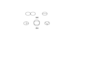
Figure 1: Two-particle irreducible graphs which contribute to the effective potential of a $\lambda\phi^{4}$ theory in the CJT formalism up to (a) two loop level and (b) three loop level. The solid line represents the full propagator.

III BEC at Hartree approximation

From the Lagrangian (3), after shifting the sigma field we can write down the tree level inverse propagators of $\sigma$, $\pi_{0}$ and $\pi_{\pm}$ respectively as

$$D^{-1}_{\sigma} = \omega^{2}_{n}+{\bf k}^{2}+m^{2}+\frac{\lambda}{2}\phi^{2},$$ (10)

$$D^{-1}_{0} = \omega^{2}_{n}+{\bf k}^{2}+m^{2}+\frac{\lambda}{6}\phi^{2},$$ (11)

$$D^{-1} = (\omega_{n}+i\mu)^{2}+{\bf k}^{2}+m^{2}+\frac{\lambda}{6}\phi^{2}.$$ (12)

The equation (12) represents the inverse propagator of $\pi_{+}$ and $\pi_{-}$. As the summation in equation (8) is symmetric over $n$ from $-\infty$ to $+\infty$, $\omega_{n}+i\mu$ and $\omega_{n}-i\mu$ are equivalent in describing the propagators of $\pi_{+}$ and $\pi_{-}$. According to the CJT formalism, the effective potential at finite temperature and finite isospin chemical potential can be written as,

$$V(\phi,G)=U(\phi)+\frac{1}{2}\int_{\beta}\ln G^{-1}_{\sigma}+\frac{1}{2}\int_{\beta}\left[D^{-1}_{\sigma}G_{\sigma}-1\right]$$ (13)

$$+ \frac{1}{2}\int_{\beta}\ln G^{-1}_{0}+\frac{1}{2}\int_{\beta}\left[D^{-1}_{0}G_{0}-1\right]+\int_{\beta}\ln G^{-1}+\int_{\beta}\left[D^{-1}G-1\right]+V_{2}(\phi,G),$$

where $G_{\sigma},G_{0}$ and $G$ are the full propagators of $\sigma,\pi_{0}$ and $\pi_{\pm}$ respectively. They are determined by the stationary condition (7). $V_{2}(\phi,G)$ represents the infinite sum of the two particle irreducible vacuum graphs. However, at the Hartree approximation we need only to calculate the “$\infty$” (or “double bubble”) diagrams and treat each loop line as the full propagator ref10 ; ref15 . Therefore, $V_{2}$ can be written as

$$V_{2}(\phi,G) = \frac{\lambda}{8}\left[\int_{\beta}G_{\sigma}\right]^{2}+\frac{\lambda}{3}\left[\int_{\beta}G\right]^{2}+\frac{\lambda}{8}\left[\int_{\beta}G_{0}\right]^{2}$$ (14)

$$+ \frac{\lambda}{6}\int_{\beta}G_{\sigma}\int_{\beta}G+\frac{\lambda}{12}\int_{\beta}G_{\sigma}\int_{\beta}G_{0}+\frac{\lambda}{6}\int_{\beta}G\int_{\beta}G_{0}.$$

For the full propagators we could take the following ansatz,

$$G^{-1}_{\sigma} = \omega^{2}_{n}+{\bf k}^{2}+M^{2}_{\sigma},$$ (15)

$$G^{-1}_{0} = \omega^{2}_{n}+{\bf k}^{2}+M^{2}_{0},$$ (16)

$$G^{-1} = (\omega_{n}+i\mu)^{2}+{\bf k}^{2}+M^{2},$$ (17)

where the effective masses $M_{\sigma},M_{0}$ and $M$ have been introduced for $\sigma,\pi_{0}$ and $\pi_{\pm}$ respectively. As in the Hartree approximation, only the tadpole diagrams contribute to the self-energies. The effective masses are independent of momentum. From the stationary condition (7), we obtain a set of effective mass gap equations,

$$M^{2}_{\sigma} = m^{2}+\frac{\lambda}{2}\phi^{2}+\frac{\lambda}{2}\int_{\beta}G_{\sigma}+\frac{\lambda}{3}\int_{\beta}G+\frac{\lambda}{6}\int_{\beta}G_{0},$$ (18)

$$M^{2}_{0} = m^{2}+\frac{\lambda}{6}\phi^{2}+\frac{\lambda}{2}\int_{\beta}G_{0}+\frac{\lambda}{6}\int_{\beta}G_{\sigma}+\frac{\lambda}{3}\int_{\beta}G,$$ (19)

$$M^{2} = m^{2}+\frac{\lambda}{6}\phi^{2}+\frac{2\lambda}{3}\int_{\beta}G+\frac{\lambda}{6}\int_{\beta}G_{\sigma}+\frac{\lambda}{6}\int_{\beta}G_{0}.$$ (20)

Accordingly the effective potential can be written as

$$V(\phi,M) = U(\phi)+\frac{1}{2}\int_{\beta}\ln G^{-1}_{\sigma}$$ (21)

$$- \frac{1}{2}\int_{\beta}(M^{2}_{\sigma}-m^{2}-\frac{\lambda}{2}\phi^{2})G_{\sigma}+\frac{1}{2}\int_{\beta}\ln G^{-1}_{0}$$

$$- \frac{1}{2}\int_{\beta}(M^{2}_{0}-m^{2}-\frac{\lambda}{6}\phi^{2})G_{0}+\int_{\beta}\ln G^{-1}$$

$$- \int_{\beta}(M^{2}-m^{2}-\frac{\lambda}{6}\phi^{2})G+V_{2}(\phi,M).$$

By minimizing the potential with respect to the order parameter $\phi$, we obtain one more equation,

$$\left[m^{2}+\frac{\lambda}{6}\phi^{2}+\frac{\lambda}{2}\int_{\beta}G_{\sigma}+\frac{\lambda}{6}\int_{\beta}G_{0}+\frac{\lambda}{3}\int_{\beta}G\right]\phi-\varepsilon=0.$$ (22)

From equations (18)—(20) and (22), the effective masses and order parameter can be solved self-consistently at given temperature and chemical potential. There are four types of integrals in above equations. After performing the Matsubara frequency sums they are

$$Q(M) = \int_{\beta}\ln[(\omega_{n}+i\mu)^{2}+{\bf k}^{2}+M^{2}]$$ (23)

$$= Q_{0}(M)+Q_{\beta}(M)$$

$$= \frac{1}{\beta}\int\frac{d^{3}{\bf k}}{(2\pi)^{3}}\frac{\omega}{2}+\frac{1}{\beta}\int\frac{d^{3}{\bf k}}{(2\pi)^{3}}\left[\ln(1-e^{-\beta(\omega+\mu)})+\ln(1-e^{-\beta(\omega-\mu)})\right],$$

$$F(M) = \int_{\beta}\frac{1}{(\omega_{n}+i\mu)^{2}+{\bf k}^{2}+M^{2}}$$ (24)

$$= F_{0}(M)+F_{\beta}(M)$$

$$= \int\frac{d^{3}{\bf k}}{(2\pi)^{3}}\frac{1}{2\omega}+\int\frac{d^{3}{\bf k}}{(2\pi)^{3}}\frac{1}{2\omega}\left[\frac{1}{e^{\beta(\omega+\mu)}-1}+\frac{1}{e^{\beta(\omega-\mu)}-1}\right],$$

$$Q(S) = \int_{\beta}\ln(\omega_{n}^{2}+{\bf k}^{2}+S^{2})$$ (25)

$$= Q_{0}(S)+Q_{\beta}(S)$$

$$= \frac{1}{\beta}\int\frac{d^{3}{\bf k}}{(2\pi)^{3}}\frac{\omega_{\bf k}}{2}+\frac{2}{\beta}\int\frac{d^{3}{\bf k}}{(2\pi)^{3}}\ln(1-e^{-\beta\omega_{\bf k}}),$$

$$F(S) = \int_{\beta}\frac{1}{\omega_{n}^{2}+{\bf k}^{2}+S^{2}}$$ (26)

$$= F_{0}(S)+F_{\beta}(S)$$

$$= \int\frac{d^{3}{\bf k}}{(2\pi)^{3}}\frac{1}{2\omega_{\bf k}}+\int\frac{d^{3}{\bf k}}{(2\pi)^{3}}\frac{1}{\omega_{\bf k}}\frac{1}{e^{\beta\omega_{\bf k}}-1},$$

where $\omega=\sqrt{{\bf k}^{2}+M^{2}}$, $\omega_{\bf k}=\sqrt{{\bf k}^{2}+S^{2}}$ and $S=M_{\sigma},M_{0}$. Each integral is divided into two parts: the zero-temperature part which is divergent and the finite- temperature part which is finite. The evaluation of the integral requires renormalization. There are some discussions concerning the renormalization on the CJT formalism in different models ref16 ; ref18 ; ref19 . The investigations about the renormalization of the $O(N)$ linear sigma model can be referred to ref11 ; ref20 . In our discussion, we only keep the finite temperature parts ($Q_{\beta}$ and $F_{\beta}$). The divergent parts of the integrals are neglected as is done in ref10 ; ref13 ; ref14 .

In the discussion of the thermodynamic system, the effective potential $V$ is equivalent to the thermodynamic potential $\Omega$. Thus we have

$$\Omega = U(\phi)+\frac{1}{2}Q_{\beta}(M_{\sigma})-\frac{1}{2}(M^{2}_{\sigma}-m^{2}-\frac{\lambda}{2}\phi^{2})F_{\beta}(M_{\sigma})$$ (27)

$$+ \frac{1}{2}Q_{\beta}(M_{0})-\frac{1}{2}(M^{2}_{0}-m^{2}-\frac{\lambda}{6}\phi^{2})F_{\beta}(M_{0})+Q_{\beta}(M)-(M^{2}-m^{2}-\frac{\lambda}{6}\phi^{2})F_{\beta}(M)+\Omega_{2},$$

where

$$\Omega_{2} = \frac{\lambda}{8}\left[F_{\beta}(M_{\sigma})\right]^{2}+\frac{\lambda}{3}\left[F_{\beta}(M)\right]^{2}+\frac{\lambda}{8}\left[F_{\beta}(M_{0})\right]^{2}$$ (28)

$$+ \frac{\lambda}{6}F_{\beta}(M_{\sigma})F_{\beta}(M)+\frac{\lambda}{12}F_{\beta}(M_{\sigma})F_{\beta}(M_{0})+\frac{\lambda}{6}F_{\beta}(M)F_{\beta}(M_{0}).$$

According to the relation

$$\rho=-\frac{\partial\Omega}{\partial\mu},$$ (29)

and equation (20), we can get the net charge density

$$\rho=\int\frac{d^{3}{\bf k}}{(2\pi)^{3}}\left[\frac{1}{e^{\beta(\omega-\mu)}-1}-\frac{1}{e^{\beta(\omega+\mu)}-1}\right].$$ (30)

This expression of density seems very similar to that of ideal gas, but actually they are different. Because here the effective mass $M$ in $\omega$ is a function of temperature and will be determined self-consistently by the gap equations.

Now we are in a position to discuss BEC. If we lower the temperature of the system from a high temperature, it is known that BEC will occur at the place where $\mu=M$ is reached. When BEC occurs, equation (30) should be written as

$$\rho=\rho_{0}+\rho^{*}(\beta,\mu=M),$$

$$\rho^{*}(\beta,\mu=M)=\int\frac{d^{3}{\bf k}}{(2\pi)^{3}}\left[\frac{1}{e^{\beta(\omega-M)}-1}-\frac{1}{e^{\beta(\omega+M)}-1}\right],$$ (31)

where $\rho_{0}$ represents the charge density of the zero-momentum state ref17 .

III.1 Chiral Limit $\varepsilon=0$

In the chiral limit ($\varepsilon=0$), the corresponding coupling constant and the negative mass parameter are given by $\lambda\approx 125$ and $-m^{2}\approx 1.8\times 10^{5}MeV^{2}$. From equation (30), when $\rho$ is fixed, by solving the gap equations (18)—(20) and equation (22), we find both $\mu$ and $M$ are functions of $T$. It can be plotted in figure 2. We can see that with $T$ decreasing, $M$ decreases first and then increases, while $\mu$ keeps increasing quickly and approaches $M$. At certain temperature, $\mu$ catches up with $M$ and BEC happens. From equation (31), we know the critical temperature $T_{c}$ is determined implicitly by the equation

$$\rho=\rho^{*}(\beta_{c},\mu=M).$$ (32)

When $T\leq T_{c}$, the system goes into BEC phase. The equation (31) will be solved together with the gap equations with $\rho$ fixed. We find $\mu$ and $M$ are still functions of $T$ and $\mu(T)=M(T)$. They both decrease with temperature decreasing, which is indicated in figure 2.

Figure 2: $\mu$ and $M$ as functions of $T$ at the fixed total charge density $\rho=0.06fm^{-3}$. BEC happens at $T_{c}=80MeV$.

For different fixed total density $\rho$, there will be different values of critical temperature $T_{c}$ and chemical potential $\mu(T_{c})$, so one can study the $\mu-T$ phase diagram of BEC. It is shown in figure 3. In the chiral limit, at $T=0$, the pion mass $M=0$, so the curve starts from the point $T=0$ and $\mu=0$. There is a disjunction at $T\approx 143MeV$. This is due to the first order chiral phase transition in the chiral limit at Hartree approximation. At low temperature $\phi\neq 0$; at certain high temperature $\phi=0$. From $\phi\neq 0$ to $\phi=0$ is discontinuous, which is reflected in the BEC phase diagram as a disjunction from low temperature to high temperature. Thorough discussion about the relation of the BEC and the chiral phase transition in the chiral limit can be referred to our previous work ref13 . In the chiral symmetry broken state ($\phi\neq 0$), the pion mass is non-zero ($\mu=M\neq 0$) which means the Nambu-Goldstone(NG) theorem is not observed at Hartree approximation as also indicated in the previous literatures ref10 ; ref21 ; ref22 . Recent discussions of this direction can be referred to ref23 ; ref24 . In this paper, we mainly discuss BEC at the usually Hartree approximation and large $N$ approximation. In our later discussion, we will see that at large $N$ approximation the NG theorem will be preserved. In figure 3, we can see clear that the whole phase plane has been divided into the BEC phase and the normal phase.

Figure 3: The phase diagram of $\mu$ versus $T$ for BEC in the chiral limit at Hartree approximation.

III.2 Non-Chiral Limit $\varepsilon\neq 0$

In the non-chiral limit ($\varepsilon\neq 0$), the corresponding coupling constant, the negative mass parameter and the explicit symmetry breaking term are given by $\lambda\approx 1.18\times 10^{2}$, $-m^{2}\approx 1.51\times 10^{5}MeV^{2}$ and $\varepsilon\approx 1.77\times 10^{6}MeV^{3}$. When equation (30) is solved together with the gap equations (18)—(20) and equation (22) at fixed $\rho$, the critical temperature $T_{c}$ of BEC will be determined at $\mu=M$ which is shown in figure 4.

Figure 4: $\mu$ and $M$ as functions of $T$ at the fixed total charge density $\rho=0.3fm^{-3}$. BEC happens at $T_{c}=132MeV$.

The procedure is similar to that of the chiral limit. For different fixed $\rho$, $\mu$ varies with $T_{c}$, so the $\mu-T$ phase diagram of BEC in the non-chiral limit can be plotted as shown in figure 5. At zero temperature, the vacuum mass of pion is $138MeV$, so the curve starts from the value of $\mu_{c}=m_{\pi}=138MeV$. The chiral phase transition in the non-chiral limit is a smooth crossover. There is no discontinuity in the BEC phase diagram.

Figure 5: The phase diagram of $\mu$ versus $T$ for BEC in the non-chiral limit at Hartree approximation.

IV BEC at large $N$ approximation

The generalized version of the meson sector of the linear sigma model is called $O(N)$ model and is based on a set of $N$ real scalar fields. The $O(N)$ model Lagrangian can be written as

$${\cal L}=\frac{1}{2}(\partial\bm{\Phi})^{2}-\frac{1}{2}m^{2}\bm{\Phi}^{2}-\frac{1}{6N}\lambda\bm{\Phi}^{2}+\varepsilon\sigma,$$ (33)

where $\bm{\Phi}$ can be identified as $\bm{\Phi}=(\sigma,\pi_{1},\pi_{2},\cdots,\pi_{N-1})$. The last term is the symmetry breaking term in order to generate the observed masses of the pions. If $N=4$, it becomes the $O(4)$ linear sigma which has been discussed above.

For the $O(N)$ linear sigma model, after introducing the chemical potential and shifting the sigma field the Lagrangian can be written as

$${\cal L} = (D_{\mu}\pi)^{+}(D^{\mu}\pi)^{-}-(m^{2}+\frac{2\lambda}{3N}\phi^{2})|\pi|^{2}+\frac{1}{2}\sum_{i}(\partial\pi_{i})^{2}+\frac{1}{2}(\partial\sigma)^{2}$$ (34)

$$- \frac{1}{2}(m^{2}+\frac{2\lambda}{3N}\phi^{2})\sum_{i}\pi^{2}_{i}-\frac{1}{2}(m^{2}+\frac{2\lambda}{N}\phi^{2})\sigma^{2}-\frac{1}{2}m^{2}\phi^{2}-\frac{\lambda}{6N}\phi^{4}+\varepsilon\phi$$

$$- \frac{\lambda}{6N}\sum_{i,j}\left[\sigma^{4}+4|\pi|^{4}+4\sigma^{2}|\pi|^{2}+2\sigma^{2}\pi_{i}^{2}+4|\pi|^{2}\pi_{i}^{2}+\pi_{i}^{4}+2\pi_{i}^{2}\pi_{j}^{2}\right]$$

where $|\pi|^{2}=\pi_{+}\pi_{-}$, the sum over $i$ or $j$ is from $3$ to $N-1$ and $i\neq j$. The chemical potential here is associated with the conserved charge of an $O(2)$ symmetry ref25 . Then we can write down the tree level inverse propagators of $\sigma$, $\pi_{i}$ and $\pi_{\pm}$ respectively as

$$D^{-1}_{\sigma} = \omega^{2}_{n}+{\bf k}^{2}+m^{2}+\frac{2\lambda}{N}\phi^{2},$$ (35)

$$D^{-1}_{i} = \omega^{2}_{n}+{\bf k}^{2}+m^{2}+\frac{2\lambda}{3N}\phi^{2},$$ (36)

$$D^{-1} = (\omega_{n}+i\mu)^{2}+{\bf k}^{2}+m^{2}+\frac{2\lambda}{3N}\phi^{2}.$$ (37)

From the CJT formalism, the thermodynamic potential of the $O(N)$ linear sigma model can be written as

$$\Omega(\phi,G)=\frac{1}{2}m^{2}\phi^{2}+\frac{\lambda}{6N}\phi^{4}-\varepsilon\phi+\frac{1}{2}\int_{\beta}\ln G^{-1}_{\sigma}+\frac{1}{2}\int_{\beta}\left[D^{-1}_{\sigma}G_{\sigma}-1\right]$$ (38)

$$+ \frac{N-3}{2}\int_{\beta}\ln G^{-1}_{i}+\frac{N-3}{2}\int_{\beta}\left[D^{-1}_{i}G_{i}-1\right]+\int_{\beta}\ln G^{-1}+\int_{\beta}\left[D^{-1}G-1\right]+\Omega_{2}(\phi,G),$$

where

$$\Omega_{2}(\phi,G) = \frac{\lambda}{2N}\left[\int_{\beta}G_{\sigma}\right]^{2}+\frac{4\lambda}{3N}\left[\int_{\beta}G\right]^{2}+\frac{(N-1)(N-3)\lambda}{6N}\left[\int_{\beta}G_{i}\right]^{2}$$ (39)

$$+ \frac{2\lambda}{3N}\int_{\beta}G_{\sigma}\int_{\beta}G+\frac{(N-3)\lambda}{3N}\int_{\beta}G_{\sigma}\int_{\beta}G_{i}+\frac{2(N-3)\lambda}{3N}\int_{\beta}G\int_{\beta}G_{i}.$$

By minimizing the thermodynamic potential with the full propagators, we obtain the following set of effective mass gap equations

$$M^{2}_{\sigma} = m^{2}+\frac{2\lambda}{N}\phi^{2}+\frac{2\lambda}{N}\int_{\beta}G_{\sigma}+\frac{4\lambda}{3N}\int_{\beta}G+\frac{2(N-3)\lambda}{3N}\int_{\beta}G_{i},$$ (40)

$$M^{2}_{i} = m^{2}+\frac{2\lambda}{3N}\phi^{2}+\frac{2(N-1)\lambda}{3N}\int_{\beta}G_{i}+\frac{2\lambda}{3N}\int_{\beta}G_{\sigma}+\frac{4\lambda}{3N}\int_{\beta}G,$$ (41)

$$M^{2} = m^{2}+\frac{2\lambda}{3N}\phi^{2}+\frac{8\lambda}{3N}\int_{\beta}G+\frac{2\lambda}{3N}\int_{\beta}G_{\sigma}+\frac{2(N-3)\lambda}{3N}\int_{\beta}G_{i},$$ (42)

where $M_{i}$ stands for the effective mass of $\pi_{i}$ ($i=3,\cdots,N-1$). By minimizing the thermodynamic potential with the order parameter $\phi$, we have one more equation

$$\left[m^{2}+\frac{2\lambda}{3N}\phi^{2}+\frac{2\lambda}{N}\int_{\beta}G_{\sigma}+\frac{2(N-3)\lambda}{3N}\int_{\beta}G_{i}+\frac{4\lambda}{3N}\int_{\beta}G\right]\phi-\varepsilon=0.$$ (43)

In the large $N$ approximation, which means that we ignore the terms of $O(1/N)$, the equations $(\ref{eq1})-(\ref{eq2})$ reduce to

$$M^{2}_{\sigma}=m^{2}+\frac{2\lambda}{N}\phi^{2}+\frac{2\lambda}{3}F_{\beta}(M_{i}),$$ (44)

$$M^{2}_{i}=m^{2}+\frac{2\lambda}{3N}\phi^{2}+\frac{2\lambda}{3}F_{\beta}(M_{i}),$$ (45)

$$M^{2}=m^{2}+\frac{2\lambda}{3N}\phi^{2}+\frac{2\lambda}{3}F_{\beta}(M_{i}).$$ (46)

$$\left[m^{2}+\frac{2\lambda}{3N}\phi^{2}+\frac{2\lambda}{3}F_{\beta}(M_{i})\right]\phi-\varepsilon=0.$$ (47)

The terms quadratic in $\phi$ are not of $O(1/N)$ but of $O(1)$ since $\phi$ depends on $N$ as $\phi^{2}=3Nm^{2}/2\lambda$. For the integration only the finite temperature part is preserved as done in Hartree approximation. The effective mass equations (45) and (46) are identical which shows the effective mass of $\pi_{\pm}$ is equal to that of $\pi_{i}$.

From the thermodynamic potential we can also derive the net charge density as

$$\rho=\int\frac{d^{3}{\bf k}}{(2\pi)^{3}}\left[\frac{1}{e^{\beta(\omega-\mu)}-1}-\frac{1}{e^{\beta(\omega+\mu)}-1}\right],$$ (48)

where $\omega=\sqrt{{\bf k}^{2}+M^{2}}$. In the following discussion we will set $N=4$ for our numerical evaluation.

IV.1 Chiral Limit $\varepsilon=0$

In the chiral limit, by the equation (46), the equation (47) could be written as

$$\phi M^{2}=0.$$ (49)

When $\phi\neq 0$, the effective mass of pion will be zero.

Figure 6: $\mu$ and $M$ as functions of $T$ at the fixed total charge density $\rho=0.1fm^{-3}$. BEC happens at $T_{c}=190MeV$.

Therefore the pions are massless Goldstone bosons in the chiral symmetry broken phase which means the NG theorem is observed in the large $N$ approximation. In chiral symmetry broken phase BEC will happen at $\mu=M=0$. At certain high temperature that the chiral symmetry restored and $\phi=0$, pion becomes massive because of the thermal contribution to the effective mass. In this case the equation (46) and (48) will be solved together at fixed density to determine the critical temperature of BEC as shown in figure 6.

Figure 7: The phase diagram of $\mu$ versus $T$ for BEC in the chiral limit at large $N$ approximation.

For different density by determining the critical temperature and chemical potential, we can plot The $\mu-T$ phase diagram of BEC as show in figure 7. At low temperature when chiral symmetry is not restored, the BEC will happen at $\mu(T)=M(T)=0$ which reflects the requirements of the NG theorem; At high temperature when chiral symmetry is restored, the BEC happens when $\mu$ equal to the nonzero effective mass of pion.

IV.2 Non-Chiral Limit $\varepsilon\neq 0$

In the non-chiral limit, the equation (46), (47) and (48) will be solved together at fixed density to find the critical temperature of BEC.

Figure 8: $\mu$ and $M$ as functions of $T$ at the fixed total charge density $\rho=0.1fm^{-3}$. BEC happens at $T_{c}=125MeV$.

The figure 8 shows the critical temperature at the fixed density is determined just at the time $\mu(T)=M(T)$. By the same procedure as that in the chiral limit, the $\mu-T$ phase diagram could be plotted as in figure 9.

Figure 9: The phase diagram of $\mu$ versus $T$ for BEC in the non-chiral limit at large $N$ approximation.

At zero temperature the vacuum mass of pion is $138MeV$, and the BEC happens at critical chemical potential $\mu_{c}=138MeV$. When temperature increases the critical chemical potential also increases. The BEC phase is in the upper plane of the phase diagram.

V summary

By the CJT formalism we have derived the temperature and density dependent effective potential based on the linear sigma model. The BEC is investigated at the Hartree approximation and the large $N$ approximation. The critical temperature of BEC is determined by lowering the temperature of the system at the fixed density to find the critical point at which $\mu(T)=M(T)$. The $\mu-T$ phase diagram of BEC has been plotted in different situations. The main features of BEC at different approximations can be summarized as below:

(1) At Hartree approximation and in chiral limit, for the $\mu-T$ phase diagram of BEC, the phase separate line is discontinuous from low temperature to high temperature. At low temperature phase ($\phi\neq 0$), BEC happens at $\mu=M\geq 0$, which shows the NG theorem is not observed.

(2)At Hartree approximation and in non- chiral limit, the critical chemical potential of BEC at zero temperature is exactly the vacuum mass of pion ($138MeV$). With temperature increasing the critical chemical potential increases continuously.

(3) At large $N$ approximation and in chiral limit, at low temperature phase before chiral symmetry restored ($\phi\neq 0$), BEC happens exactly at $\mu(T)=M(T)=0$, which shows the NG theorem is observed. Above certain temperature when chiral symmetry is restored, the critical chemical potential of BEC becomes non-zero and increases with temperature increasing.

(4) At large $N$ approximation and in non-chiral limit, the critical chemical potential of BEC is $138MeV$ at zero temperature then increases with temperature increasing.

References

(1)
Son D T and Stephanov M A 2001 Phys.Rev.Lett.86 592
(2)
Kogut J B and Toublan D 2001 Phys. Rev. D 64 034007
(3)
Loewe M and Villavicencio C 2003 Phys. Rev. D 67
074034
(4)
Kogut J B and Sinclair D K 2002 Phys. Rev. D 66 014508
(5)
Kogut J B and Sinclair D K 2004 Phys. Rev. D 70 094501
(6)
Toublan D and Kogut J B 2003 Phys. Lett. B 564 212
(7)
Barducci A, Casalbuoni R, Pettini G and Ravagli L 2005 Phys.
Rev. D 71 016011
(8)
He L Y, Jin M and Zhuang P F 2005 Phys. Rev. D 71
116001
(9)
Barducci A, Casalbuoni R, Pettini G and Ravagli L 2003 Phys.
Lett. B 564 217
(10)
Petropoulos N 1999 J. Phys. G 25 2225
(11)
Lenaghan J and Rischke D 2000 J. Phys. G 26 431
(12)
Scavenius O et al 2001 Phys. Rev. C 64 045202
(13)
Shu S and Li J R 2005 J. Phys. G 31 459
(14)
Mao H, Petropoulos N, Shu S and Zhao W Q 2006 J. Phys. G
32 2187
(15)
Cornwall J, Jackiw R and Tomboulis E 1974 Phys. Rev. D 10 2428
(16)
Amelino-Camelia G and Pi So-Young 1993 Phys. Rev. D 47
2356
(17)
Kapusta J 1989 Finite-Temperature Field Theory (Cambridge
Univ. Press)
(18)
Amelino-Camelia G 1997 Phys. Lett. B 407 268
(19)
Amelino-Camelia G 1996 Nucl. Phys. B 476 255
(20)
Lenaghan J and Rischke D and Schaffner-Bielich J 2000 Phys.
Rev. D 62 085008
(21)
Baym G and Grinstein G 1977 Phys. Rev. D 10 2897
(22)
Randrup 1997 Phys. Rev. D 55 1188
(23)
Hees H and Knoll J 2002 Phys. Rev. D 66 025028
(24)
Ivanov Y B, Riek F, Hees H and Knoll J 2005 Phys. Rev. D
72 036008
(25)
Haber H and Weldon H 1982 Phys. Rev. D 25 502