Gravitino production in the Randall-Sundrum II braneworld cosmology

Abstract

Braneworld modifications to the Friedmann expansion law can have an important effect on the cosmological evolution of the early universe. In particular, the primordial particle abundances crucially depend on the rate at which the universe expanded at early times. In this article, we study the production of stable and unstable gravitinos, both from thermal creation and from the decay of a heavy scalar, in the Randall-Sundrum II braneworld context. We conclude that, depending on the value of the 5D fundamental Planck mass, some of the usual standard cosmology constraints on the reheating temperature and on the mass of the heavy scalar can be evaded.

I Introduction

The (over)production of gravitinos can have striking impact on cosmology Khlopov and Linde (1984). If gravitinos are unstable, their overabundance would spoil the success of big-bang nucleosynthesis (BBN). On the other hand, if they are stable particles, which is the case if they are the lightest supersymmetric particle (LSP) contributing to the total amount of dark matter, the present abundance of gravitinos is constrained in order to avoid the overclosure of the universe.

It is long known that gravitinos can be thermally produced through scatterings in the plasma. However, it has been recently pointed out Endo et al. (2006a); Nakamura and Yamaguchi (2006), in the context of the moduli problem Coughlan et al. (1983), that the decay rate of the scalar field into a pair of gravitinos is much higher than previously thought Hashimoto et al. (1998). This “new” source of gravitinos coming from a scalar field decay might have important consequences for the evolution of the universe. In fact, we expect that the universe was once dominated by a scalar field, for example, the inflaton (see, e.g., Ref. Lyth and Riotto (1999) for a review), or the dilaton and moduli fields in superstring theories. The production of gravitinos from inflaton/dilaton/scalar decays, and the problems that might result, have been widely studied in standard cosmology (SC) Endo et al. (2006a); Nakamura and Yamaguchi (2006); Kawasaki et al. (2006a, b); Asaka et al. (2006); Endo et al. (2006b, c); Dine et al. (2006).

In the last years, there has also been much interest in the so-called braneworld cosmology (BC) scenarios. Whilst theories formulated in extra dimensions have been around since the early twentieth century, recent developments in string theory have opened up the possibility that our universe could be a 1+3-surface, the brane, embedded in a higher-dimensional space-time, called the bulk, with all (minimal supersymmetric) standard model particles and fields trapped on the brane, while gravity is free to access the bulk (see Ref. Maartens (2004) for a review). A remarkable feature of BC is the modification of the expansion rate of the universe before the BBN era. In the so-called Randall-Sundrum II (RSII) braneworld construction Randall and Sundrum (1999), in which one has a single brane with positive tension $\lambda$, the Friedmann equation receives an additional term quadratic in the density Binetruy et al. (2000a); Csaki et al. (1999); Cline et al. (1999); Shiromizu et al. (2000); Binetruy et al. (2000b); Kraus (1999); Ida (2000); Mukohyama et al. (2000). Setting the 4D cosmological constant to zero and assuming that inflation rapidly makes any dark radiation term negligible, one obtains

$$H^{2}=\frac{8\pi}{3M_{P}^{2}}~{}\rho~{}\left(1+\frac{\rho}{2\lambda}\right)~{},\quad\quad M_{P}=\sqrt{\frac{3}{4\pi}}\frac{M_{5}^{3}}{\sqrt{\lambda}}~{},$$ (1)

where $M_{P}=1.22\times 10^{19}$ GeV is the 4D Planck mass and $M_{5}$ the 5D fundamental mass. Notice that Eq. (1) reduces to the usual Friedmann equation, $H\propto\sqrt{\rho}$, at sufficiently low energies, $\rho\ll\lambda$, but at very high energies one has $H\propto\rho$. Successful BBN requires that the change in the expansion rate due to the new terms in the Friedmann equation be sufficiently small at scales $\sim\mathcal{O}$(MeV); this implies $M_{5}\gtrsim 40~{}\mbox{TeV}$. A more stringent bound, $M_{5}\gtrsim 10^{5}~{}\mbox{TeV}$, is obtained by requiring the theory to reduce to Newtonian gravity on scales larger than 1 mm.

As is well known, the above modification in the Friedmann expansion rate can have important implications for inflation Maartens et al. (2000), baryogenesis Mazumdar (2001); Bento et al. (2004c), dark matter Okada and Seto (2004) and thermal gravitino production Okada and Seto (2005). In this paper we aim to investigate its effect in the decay of a heavy scalar field into a pair of gravitinos. After a brief discussion on the decay of heavy scalars and the production of gravitinos in the RSII brane scenario, we study the resulting constraints on the parameter space, both for the stable and unstable gravitino cases.

II Heavy scalar decay and RSII cosmology

We consider here the case in which the scalar particle $X$ dominates the energy of the universe when it decays, $\rho\simeq\rho_{X}$. This scenario can be achieved if the scalar is, for example, the inflaton. We will assume that $X$ is a singlet under the standard model gauge group.

Of particular interest is the reheating temperature, $T_{rh}$, which is defined here by assuming an instantaneous conversion of $X$ energy into radiation, when the decay width of $X$, $\Gamma_{X}$, equals the expansion rate of the universe. If the total energy density of the scalar $X$ is instantaneously converted into radiation, then we can identify $\rho_{X}=\rho_{R}=(\pi^{2}/30)\,g_{\ast}\,T^{4}\,$, where $g_{\ast}$ is the effective number of relativistic degrees of freedom at the temperature $T$. In particular, $g_{\ast}=915/4=228.75$ in the minimal supersymmetric standard model (MSSM), for temperatures above the SUSY breaking scale $\sim\mathcal{O}$(TeV). For a radiation dominated universe, Eq. (1) can then be written as

$$H^{2}=H_{SC}^{2}(T)\left[1+\left(\dfrac{T}{T_{t}}\right)^{4}\right]~{},$$ (2)

where

$$H_{SC}(T)=\dfrac{2\pi}{3}\,\sqrt{\dfrac{\pi\,g_{*}}{5}}\;\dfrac{T^{2}}{M_{P}}~{}$$ (3)

is the usual SC expansion law, and we have defined

$$T_{t}=\left(\dfrac{45M_{5}^{6}}{\pi^{3}g_{*}M_{P}^{2}}\right)^{1/4}=8.1\times 10^{4}\,{\rm GeV}\,\left(\dfrac{M_{5}}{10^{10}\,{\rm GeV}}\right)^{3/2}~{},$$ (4)

as the transition temperature from the high energy brane regime expansion to the standard expansion. From the condition

$$H(T_{rh})=\Gamma_{X}$$ (5)

one gets the reheating temperature $T_{rh}$, where $\Gamma_{X}$ is the total decay rate of $X$. In the high-energy limit of BC, i.e. for $T\gg T_{t}$, Eq. (2) reads

$$H_{BC}\simeq\frac{2\pi^{3}g_{\ast}}{45}\frac{T^{4}}{M_{5}^{3}}~{},$$ (6)

and the condition in Eq. (5) leads then to the relation

$$T_{rh}=\left(\frac{45}{2\pi^{3}g_{\ast}}\Gamma_{X}M_{5}^{3}\right)^{1/4}~{}.$$ (7)

In the SC limit ($T\ll T_{t}$) one obtains

$$T_{rh}=\left(\frac{45}{4\pi^{3}g_{\ast}}\right)^{1/4}\sqrt{\Gamma_{X}M_{P}}~{}.$$ (8)

The total decay rate of $X$ is determined from all the interactions of $X$ with the other particles of the supersymmetric model, and so it is model dependent. However we can in general write

$$\Gamma_{X}=\alpha_{t}^{2}\,\dfrac{M_{X}^{3}}{M_{P}^{2}}~{}.$$ (9)

In fact, when $X$ has only Planck suppressed interaction, $\alpha_{t}$ is expected to be of order one. For example, if $X$ is the heavy moduli field that couples to gauge supermultiplets in the gauge kinetic function through a Planck suppressed interaction, the decay rate of $X$ is of the form of Eq. (9) with $\alpha_{t}={\cal O}(1)$ Endo et al. (2006a); Nakamura and Yamaguchi (2006).

Using Eq. (9), the reheating temperature in the BC regime can be written as

$$T_{rh}=6.8\times 10^{4}\,{\rm GeV}\,\alpha_{t}^{1/2}\left(\dfrac{M_{X}}{10^{10}\,{\rm GeV}}\right)^{3/4}\left(\dfrac{M_{5}}{10^{10}\,{\rm GeV}}\right)^{3/4}~{},$$ (10)

while in the SC limit one obtains

$$T_{rh}=5.7\times 10^{4}\,{\rm GeV}\,\alpha_{t}\left(\dfrac{M_{X}}{10^{10}\,{\rm GeV}}\right)^{3/2}~{}.$$ (11)

At this point one should notice that $T_{rh}>7$ MeV in order to be consistent with BBN theory. This implies that in BC regime the relation $M_{X}M_{5}\gtrsim 4.8\times 10^{10}\,\alpha_{t}^{-2/3}\,{\rm GeV}^{2}$ should be satisfied, while in SC one should have $M_{X}\gtrsim 2.5\times 10^{5}\,\alpha_{t}^{-2/3}\,{\rm GeV}$. However, in order to have the BC regime one should also impose $T_{rh}>T_{t}$, i.e. to obtain such a low reheating temperature in the BC regime one needs also a low $T_{t}$ which corresponds to a low value of $M_{5}$. Such low values of $M_{5}$ are not compatible with the bound $M_{5}\gtrsim 10^{5}~{}\mbox{TeV}$, obtained by requiring the theory to reduce to Newtonian gravity on scales larger than 1 mm. This implies that the only relevant bound is coming from the SC regime

$$M_{X}\gtrsim 2.5\times 10^{5}\,{\rm GeV}~{}\dfrac{1}{\alpha_{t}^{2/3}}~{}.$$ (12)

One should also point out that in order to have $T_{rh}>T_{t}$, one must impose

$$M_{X}>\left(\dfrac{2}{\alpha_{t}^{2}}\right)^{1/3}M_{5}~{}.$$ (13)

Here we are mainly interested in the gravitino production, and hence in the decay of a heavy scalar field $X$ into a pair of gravitinos

$$X\rightarrow\psi_{3/2}+\psi_{3/2}~{}.~{}$$ (14)

Before we proceed with the discussion of the decay of the heavy scalar into gravitinos, we should specify better our brane setup, namely the localization of gravitinos on the brane. We are considering here the supersymmetric extension of the RSII braneworld model Gherghetta and Pomarol (2000). As already mentioned, in the Randall-Sundrum construction under consideration, only gravity propagates in the bulk: the zero-mode graviton is localized around the ultraviolet (UV) brane (our brane), while the graviton Kaluza-Klein (KK) modes are localized around the infrared brane (which in the RSII is located at the infinite boundary). In the supersymmetric generalization, all the fields in the same supermultiplet will take the same configuration in the fifth dimensional direction. Hence, the zero-mode gravitino will also be localized around the UV brane. As an approximation we will consider it as a field residing on the UV brane, as done previously in other works Okada and Seto (2005); Bento et al. (2004c). The zero-mode gravitino will obtain its mass through the super-Higgs mechanism, as in the usual 4D supergravity. Since supersymmetry is broken only locally on the UV brane, the KK gravitinos will remain the same. We will not consider here the production of these KK gravitinos and its possible influence on the brane particle content. We will only consider the zero-mode gravitino as a field residing on the brane and apply 4D supersymmetry and the usual Boltzmann equation to describe its production.

Let us now briefly discuss the decay channel in Eq. (14). For simplicity, we will assume that $M_{X}>>m_{3/2}$. In fact, the gravitino is likely to be much lighter than either a heavy modulus or the inflaton, because a too large gravitino mass requires a fine-tuning in the Higgs sector due to the anomaly-mediated effects. With this assumption, the decay rate for this process, as recently calculated in Refs. Endo et al. (2006a); Nakamura and Yamaguchi (2006), can be written as

$$\Gamma_{3/2}=\dfrac{\alpha_{3/2}^{2}}{36}\dfrac{M_{X}^{3}}{M_{P}^{2}}~{}.$$ (15)

The coupling constant $\alpha_{3/2}$ is defined by the relation

$$\alpha_{3/2}\,\,\dfrac{M_{3/2}^{2}}{M_{X}}=\left\langle\left(G_{X\overline{X}}\right)^{-1/2}e^{G/2}\,G_{X}\right\rangle~{},$$ (16)

with $G$ being the total Kähler potential, $G=K+\ln|W|^{2}$, where $K$ and $W$ are the Kähler potential and the superpotential, respectively. The subscript $X$ ($\overline{X}$) denotes differentiation with respect to the $X$ ($\overline{X}$) field and $\langle\,...\;\rangle$ stands for the VEV. In general one has Kawasaki et al. (2006a, b); Asaka et al. (2006); Endo et al. (2006a); Nakamura and Yamaguchi (2006); Endo et al. (2006c, b)

$$\alpha_{3/2}=c\;\dfrac{\left|\left\langle X\right\rangle\right|}{M_{P}}~{},$$ (17)

where the value of the constant $c$ depends on the explicit model. For example, in the scenario discussed in Ref. Kawasaki et al. (2006a), one has $c=\sqrt{3}$. For a moduli field, $\alpha_{3/2}$ is expected to be order unity Asaka et al. (2006), and hence the decay of the moduli field into a pair of gravitinos can be significant, thus leading to cosmological disasters. If $X$ is the inflaton, then $\alpha_{3/2}$ can take values much smaller than unity, as in some new and hybrid inflationary models. If $\alpha_{3/2}$ is zero then no gravitinos are produced in the decay of $X$. This is what happens in the simplest chaotic inflationary models, for which $G_{X}=0$ in the vacuum (see Ref. Asaka et al. (2006); Kawasaki et al. (2006b); Endo et al. (2006b)). In the following we will leave $\alpha_{3/2}$ as a free parameter.

One should note that the expression in Eq. (15) for the decay rate of the gravitino cannot be applicable for $H>m_{3/2}$. As pointed out in Kawasaki et al. (2006b), the decay proceeds only if the Hubble parameter is smaller than the gravitino mass, since the chirality flip of the gravitino forbids the decay to proceed otherwise. This imposes a bound on the maximum value that $M_{X}$ can take, and also on the maximum reheating temperature. The condition $H(T_{rh})<m_{3/2}$ is, by the definition of $T_{rh}$ [cf. Eq. (5)], the same as $\Gamma_{X}<m_{3/2}$. Hence

$$2.5\times 10^{5}\,{\rm GeV}\,\alpha_{t}^{-2/3}\lesssim M_{X}\lesssim 5.3\times 10^{13}\,{\rm GeV}\,\alpha_{t}^{-2/3}\,\left(\dfrac{m_{3/2}}{10^{3}~{}{\rm GeV}}\right)^{1/3}~{},$$ (18)

where the first inequality is the one already presented in Eq. (12). The upper bound on the reheating temperature turns out to be

$$T_{rh}\lesssim 4.2\times 10^{7}\,{\rm GeV}\left(\dfrac{m_{3/2}}{10^{3}~{}{\rm GeV}}\right)^{1/4}\left(\dfrac{M_{5}}{10^{10}~{}{\rm GeV}}\right)^{3/4}$$ (19)

in the high-energy brane regime, and

$$T_{rh}\lesssim 2.2\times 10^{10}\,{\rm GeV}\left(\dfrac{m_{3/2}}{10^{3}~{}{\rm GeV}}\right)^{1/2}$$ (20)

in the SC limit.

Summarizing, one would expect that the brane effects will change the gravitino production for reheating temperatures in the range

$$8.1\times 10^{4}\,{\rm GeV}\,\left(\dfrac{M_{5}}{10^{10}\,{\rm GeV}}\right)^{3/2}\lesssim T_{rh}\lesssim 4.2\times 10^{7}\,{\rm GeV}\left(\dfrac{m_{3/2}}{10^{3}~{}{\rm GeV}}\right)^{1/4}\left(\dfrac{M_{5}}{10^{10}~{}{\rm GeV}}\right)^{3/4}$$ (21)

or, equivalently, heavy scalar masses in the interval

$$\left(\dfrac{2}{\alpha_{t}^{2}}\right)^{1/3}M_{5}\,\lesssim\,M_{X}\,\lesssim\,5.3\times 10^{13}\,{\rm GeV}\,\alpha_{t}^{-2/3}\,\left(\dfrac{m_{3/2}}{10^{3}~{}{\rm GeV}}\right)^{1/3}~{}.$$ (22)

III Gravitino Abundance

As referred in the Introduction, a viable cosmological supergravity-inspired scenario has to avoid the so-called gravitino problem. For unstable gravitinos, their decay products should not alter the BBN predictions for the abundance of light elements in the universe. On the other hand, if they are stable particles they will contribute to the dark matter content, and thus one has to avoid the overclosure of the universe.

In the following we will estimate the contributions to the gravitino abundance, both from thermal production and from the decay of a heavy scalar. Then we will discuss the constraints coming for stable or unstable gravitinos.

III.1 Brane cosmology vs standard cosmology

Gravitinos can be produced by the decay of the heavy scalar particle $X$, and, during the reheating phase, they are also thermally produced through scatterings in the plasma. The total abundance is then given by both contributions

$$Y_{3/2}\equiv\frac{n_{3/2}}{s}=Y_{3/2}^{Th}+Y_{3/2}^{X}~{},$$ (23)

where $s(T)=2\pi^{2}g_{*}T^{3}/45$ is the entropy density, and $Y_{3/2}^{Th(X)}$ stands for the contribution from thermal scatterings ($X$ decay) to the total gravitino abundance.

Let us estimate the contribution of thermal scatterings at reheating. The gravitino abundance at a given temperature $T<T_{rh}$ is obtained from the Boltzmann equation

$$\frac{dn_{3/2}}{dt}+3Hn_{3/2}=C_{3/2}(T)~{},$$ (24)

where $C_{3/2}(T)$ is the collision term given by Bolz et al. (2001)

$$C_{3/2}(T)\simeq\alpha(T)\left(1+\beta(T)\frac{m_{{\tilde{g}}}^{2}}{m_{3/2}^{2}}\right)\frac{T^{6}}{M_{P}^{2}}~{},$$ (25)

where $m_{{\tilde{g}}}$ is the low-energy gluino mass; $\alpha(T)$ and $\beta(T)$ are slowly-varying functions of the temperature. Assuming constant entropy, the integration of Eq. (24) yields

$$Y_{3/2}^{Th}\simeq{\cal A}(T;m_{3/2},m_{{\tilde{g}}})\left(2\,T_{t}-\dfrac{T_{t}^{2}}{T_{rh}}-T\right)~{},$$ (26)

with

$${\cal A}(T;m_{3/2},m_{{\tilde{g}}})=\left(\dfrac{45}{\pi g_{*}}\right)^{3/2}\dfrac{\alpha(T)}{4\pi^{2}M_{P}}\left(1+\beta(T)\frac{m_{{\tilde{g}}}^{2}}{m_{3/2}^{2}}\right)~{}.$$ (27)

This is an approximate solution, obtained by integrating the Boltzmann equation in the BC regime for $T_{rh}>T>T_{t}$ and the SC limit for $T<T_{t}$, considering a small dependence of ${\cal A}(T;m_{3/2},m_{{\tilde{g}}})$ on the temperature. In Ref. Okada and Seto (2005), an analytic solution in terms of a Gauss hypergeometric function was found. However the result presented in Eqs. (26) and (27) is, for our purposes, a very good approximation.

In the high energy limit of BC, Eq. (26) leads to

$$Y_{3/2}^{Th}\simeq 2\,{\cal A}(T_{t};m_{3/2},m_{{\tilde{g}}})\,T_{t}~{},$$ (28)

while in the SC limit one obtains the usual result

$$Y_{3/2}^{Th}\simeq{\cal A}(T_{rh};m_{3/2},m_{{\tilde{g}}})\,T_{rh}~{}.$$ (29)

In the BC regime, the abundance of gravitinos produced by thermal scatterings is proportional to the transition temperature instead of the reheating temperature. This has been proposed as a possible solution for the thermal gravitino problem in the context of supersymmetric thermal leptogenesis Okada and Seto (2005): in SC, the gravitino bound imposed on the reheating temperature, $T_{rh}\lesssim 10^{6}-10^{10}$ GeV (depending on the gravitino mass and the hadronic branching ratio Kohri et al. (2006); Kawasaki et al. (2006b); Endo et al. (2006b)), is barely compatible with the simplest models of supersymmetric thermal leptogenesis which need $T_{rh}\gtrsim 10^{7}-10^{9}$ GeV.

Let us now look at the contribution of the decay process (14) to the total gravitino abundance [cf. Eq. (23)]. The amount of gravitinos produced by this process can be written as

$$Y_{3/2}^{X}=\dfrac{3}{2}\,B_{3/2}\,\dfrac{T_{rh}}{M_{X}}~{},$$ (30)

where

$$B_{3/2}\equiv\dfrac{\Gamma_{3/2}}{\Gamma_{X}}=\dfrac{\alpha_{3/2}^{2}}{36\,\alpha_{t}^{2}}$$ (31)

is the branching ratio of the decay channel (14). If $\alpha_{3/2}\ll 1$ (or/and $\alpha_{t}\gg 1$), $B_{3/2}$ can be much smaller than unity.

The abundance of gravitinos produced from the decay of $X$ can then be written as

$$Y_{3/2}^{X}=\dfrac{\alpha_{3/2}^{2}}{24\,\alpha_{t}^{2}}\,\dfrac{T_{rh}}{M_{X}}=\dfrac{\alpha_{3/2}^{2}\,M_{X}^{2}\,T_{rh}}{24\,H(T_{rh})\,M_{P}^{2}}~{}.$$ (32)

Notice that, in the brane scenario, $H(T_{rh})$ is in fact a function of $T_{rh}$ and $T_{t}$ (or $M_{5}$). In the BC and SC limits, this equation leads, respectively, to

$$Y_{3/2}^{X} =8.9\times 10^{-11}\,\alpha_{3/2}^{2}\left(\dfrac{M_{X}}{10^{10}~{}{\rm GeV}}\right)^{2}\left(\dfrac{M_{5}}{10^{10}~{}{\rm GeV}}\right)^{3}\left(\dfrac{T_{rh}}{10^{6}~{}{\rm GeV}}\right)^{-3}$$

$$=1.0\times 10^{-5}\,B_{3/2}\,\alpha_{t}^{1/2}\left(\dfrac{M_{5}}{10^{10}~{}{\rm GeV}}\right)^{3/4}\left(\dfrac{M_{X}}{10^{10}~{}{\rm GeV}}\right)^{-1/4}~{},$$ (33)

and

$$Y_{3/2}^{X} =1.4\times 10^{-8}\,\alpha_{3/2}^{2}\left(\dfrac{M_{X}}{10^{10}~{}{\rm GeV}}\right)^{2}\left(\dfrac{T_{rh}}{10^{6}~{}{\rm GeV}}\right)^{-1}$$

$$=8.6\times 10^{-6}\,B_{3/2}\,\alpha_{t}\left(\dfrac{M_{X}}{10^{10}~{}{\rm GeV}}\right)^{1/2}~{}.$$ (34)

Note that in both regimes the gravitino abundance is inversely proportional to $T_{rh}$, in opposition to the thermal abundance in SC.

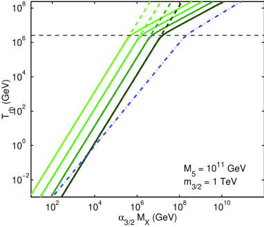
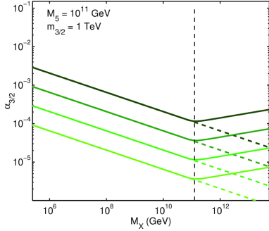
Figure 1: (Color online) Contours of constant $Y_{3/2}^{X}=10^{-17},\,10^{-16},\,10^{-15},\,10^{-14}$ (from lighter to darker green) in the $T_{rh}-\alpha_{3/2}M_{X}$ and $\alpha_{3/2}-M_{X}$ planes, for BC with $M_{5}=10^{11}$ GeV (full lines) and SC (dashed lines). The (black) horizontal dashed line in the left panel represents the value of $T_{t}$; the (black) vertical line in the right panel shows the value of $M_{X}=\left(2/\alpha_{t}^{2}\right)^{1/3}M_{5}$. The (blue) dash-dotted line represents the lower bound on $T_{rh}$ from $B_{3/2}\leq 1$ for $\alpha_{3/2}=10^{-10}$. The gravitino mass is taken to be $m_{3/2}=1$ TeV and, in the right panel, we fixed $\alpha_{t}=1$. The maximum values for $T_{rh}$ and $M_{X}$ shown in the plots are the ones given by the upper bounds of Eqs. (21) and (22), respectively.

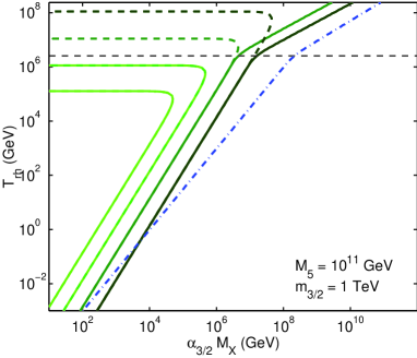
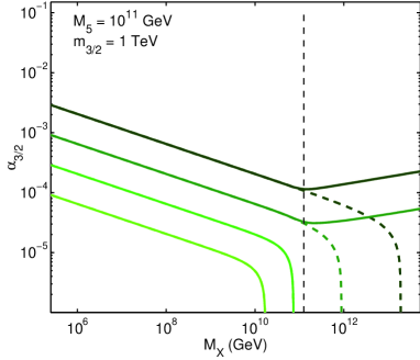
Figure 2: (Color online) Same as in Fig. 1, but for the total abundance of gravitinos: $Y_{3/2}=10^{-17},\,10^{-16},\,10^{-15},\,10^{-14}$ (from lighter to darker green). In the computation of the thermal abundance, the gluino mass was taken to be $m_{{\tilde{g}}}=1$ TeV.

In Fig. 1 we present the contours of constant $Y_{3/2}^{X}$ in the $T_{rh}-\alpha_{3/2}M_{X}$ and $\alpha_{3/2}-M_{X}$ planes. We show the SC case (dashed lines) and the BC one (full lines), for a fixed value of $M_{5}$ ($M_{5}=10^{11}$ GeV). We have chosen the gravitino mass to be $m_{3/2}=1$ TeV. In the right panel, we see the change of behavior in the contours for $M_{X}>\left(2/\alpha_{t}^{2}\right)^{1/3}M_{5}$, for which the high-energy regime of BC is valid. This regime occurs for $T_{rh}$ larger than $T_{t}$, as we can see on the left panel. For the contour plot in the $\alpha_{3/2}-M_{X}$ plane we have chosen $\alpha_{t}=1$. One should notice that if we fix $\alpha_{t}$ at a smaller value, then the lines of constant $Y_{3/2}^{X}$ would move downwards, i.e. only smaller values of $\alpha_{3/2}$ would be allowed.

In the left panel plot, the lower bound on $T_{rh}$ from $B_{3/2}\leq 1$ is also shown by choosing $\alpha_{3/2}=10^{-10}$ (dash-dotted line). This bound can be derived from Eq. (31), which can also be rewritten as

$$B_{3/2}=\dfrac{\alpha_{3/2}^{2}\,M_{X}^{3}}{36\,H(T_{rh})\,M_{P}^{2}}~{},$$ (35)

and that in the high-energy limit of BC reads

$$B_{3/2}=5.9\times 10^{-7}\,\alpha_{3/2}^{2}\left(\dfrac{M_{5}}{10^{10}~{}{\rm GeV}}\right)^{3}\left(\dfrac{M_{X}}{10^{10}~{}{\rm GeV}}\right)^{3}\left(\dfrac{T_{rh}}{10^{6}~{}{\rm GeV}}\right)^{-4}~{}.$$ (36)

This leads to

$$T_{rh}\geq 4.9\,\alpha_{3/2}^{-1/4}\,\left(\dfrac{M_{5}}{10^{10}~{}{\rm GeV}}\right)^{3/4}\,\left(\dfrac{\alpha_{3/2}\,M_{X}}{10^{5}~{}{\rm GeV}}\right)^{3/4}~{}.$$ (37)

In SC one has

$$B_{3/2}=9.1\times 10^{-5}\,\alpha_{3/2}^{2}\left(\dfrac{M_{X}}{10^{10}~{}{\rm GeV}}\right)^{3}\left(\dfrac{T_{rh}}{10^{6}~{}{\rm GeV}}\right)^{-2}~{},$$ (38)

and hence

$$T_{rh}\geq 3.0\times 10^{-4}\,\alpha_{3/2}^{-1/2}\,\left(\dfrac{\alpha_{3/2}\,M_{X}}{10^{5}~{}{\rm GeV}}\right)^{3/2}~{}.$$ (39)

Of course, if one requires a smaller value for $B_{3/2}$, a larger value of the reheating temperature is needed. And if $\alpha_{3/2}$ is larger, the bound will be less stringent, in both cases, for a fixed $\alpha_{3/2}\,M_{X}$.

In Fig. 2 we show the contours of constant $Y_{3/2}=Y_{3/2}^{Th}+Y_{3/2}^{X}$ in the same plane as in Fig. 1, assuming $m_{{\tilde{g}}}=1$ TeV in the computation of the thermal contribution to the gravitino abundance (hereafter we will consider this mass for the gluino). In the right panel, we see that in the SC regime, i.e. for $M_{X}<\left(2/\alpha_{t}^{2}\right)^{1/3}M_{5}$, the heavy scalar mass $M_{X}$ has an upper bound (coming from the thermal production contribution), which corresponds to the upper bound on the reheating temperature (see left panel). These bounds can be easily derived from Eq. (29), which can be rewritten as

$$Y_{3/2}^{th} \simeq 10^{-16}\left[\dfrac{{\cal A}(T_{rh};m_{3/2},m_{{\tilde{g}}})}{10^{-22}~{}{\rm GeV}^{-1}}\right]\left(\dfrac{T_{rh}}{10^{6}~{}{\rm GeV}}\right)$$

$$\simeq 5.7\times 10^{-18}\,\alpha_{t}\,\left[\dfrac{{\cal A}(T_{rh};m_{3/2},m_{{\tilde{g}}})}{10^{-22}~{}{\rm GeV}^{-1}}\right]\left(\dfrac{M_{X}}{10^{10}~{}{\rm GeV}}\right)^{3/2}~{},$$ (40)

from which one gets

$$T_{rh}\lesssim 10^{6}~{}{\rm GeV}\left[\dfrac{{\cal A}(T_{rh};m_{3/2},m_{{\tilde{g}}})}{10^{-22}~{}{\rm GeV}^{-1}}\right]^{-1}\left(\dfrac{Y_{3/2}^{BBN}}{10^{-16}}\right)~{},$$ (41)

and

$$M_{X}\lesssim 6.7\times 10^{10}~{}{\rm GeV}\,\alpha_{t}^{-2/3}\,\left[\dfrac{{\cal A}(T_{rh};m_{3/2},m_{{\tilde{g}}})}{10^{-22}~{}{\rm GeV}^{-1}}\right]^{-2/3}\left(\dfrac{Y_{3/2}^{BBN}}{10^{-16}}\right)^{2/3}~{}.$$ (42)

On the other hand, in order to avoid the overproduction of gravitinos by $X$ decays, the coupling constant $\alpha_{3/2}$ has to satisfy

$$\alpha_{3/2}\lesssim 2.1\times 10^{-5}\,\alpha_{t}^{1/2}\left(\dfrac{M_{X}}{10^{10}~{}{\rm GeV}}\right)^{-1/4}\left(\dfrac{Y_{3/2}^{BBN}}{10^{-16}}\right)^{1/2}~{},$$ (43)

or, in terms of the branching ratio,

$$B_{3/2}\lesssim 1.2\times 10^{-11}\,\alpha_{t}^{-1}\left(\dfrac{M_{X}}{10^{10}~{}{\rm GeV}}\right)^{-1/2}\left(\dfrac{Y_{3/2}^{BBN}}{10^{-16}}\right)~{},$$ (44)

as already derived in Asaka et al. (2006).

For $M_{X}\gtrsim\left(2/\alpha_{t}^{2}\right)^{1/3}M_{5}$, or equivalently $T_{rh}>T_{t}$, the high-energy regime of BC holds. In this regime, the upper bound on the $T_{rh}$ disappears. Indeed, this bound is due to the thermal production of gravitinos, and, as can be seen from Eq. (28), the abundance of gravitinos produced thermally is proportional to $T_{t}$,

$$Y_{3/2}^{th} \simeq 2\times 10^{-16}\left[\dfrac{{\cal A}(T_{t};m_{3/2},m_{{\tilde{g}}})}{10^{-22}~{}{\rm GeV}^{-1}}\right]\left(\dfrac{T_{t}}{10^{6}~{}{\rm GeV}}\right)$$

$$\simeq 1.6\times 10^{-17}\,\left[\dfrac{{\cal A}(T_{t};m_{3/2},m_{{\tilde{g}}})}{10^{-22}~{}{\rm GeV}^{-1}}\right]\left(\dfrac{M_{5}}{10^{10}~{}{\rm GeV}}\right)^{3/2}~{}.$$ (45)

Hence, in the high-energy regime the bound on the reheating temperature is replaced by a bound on the transition temperature,

$$T_{t}\lesssim 5\times 10^{5}~{}{\rm GeV}\left[\dfrac{{\cal A}(T_{t};m_{3/2},m_{{\tilde{g}}})}{10^{-22}~{}{\rm GeV}^{-1}}\right]^{-1}\left(\dfrac{Y_{3/2}^{BBN}}{10^{-16}}\right)~{},$$ (46)

or, equivalently, on the 5D fundamental mass $M_{5}$

$$M_{5}\lesssim 3.4\times 10^{10}\,{\rm GeV}\,\left[\dfrac{{\cal A}(T_{t};m_{3/2},m_{{\tilde{g}}})}{10^{-22}~{}{\rm GeV}^{-1}}\right]^{-2/3}\left(\dfrac{Y_{3/2}^{BBN}}{10^{-16}}\right)^{2/3}~{}.$$ (47)

This is also reflected in the disappearance of the upper bound on the mass of the heavy scalar imposed by the limits on the gravitino abundance, and the only bound that remains on this quantity is the one in Eq. (18), which comes from requiring $m_{3/2}>H$. In fact, in this regime, in order to avoid overproduction of gravitinos in the $X$ decay, one must have

$$T_{rh}\gtrsim 4.5\times 10^{4}\left(\dfrac{\alpha_{3/2}\,M_{X}}{10^{5}~{}{\rm GeV}}\right)^{2/3}\left(\dfrac{M_{5}}{10^{10}~{}{\rm GeV}}\right)\left(\dfrac{Y_{3/2}^{BBN}}{10^{-16}}\right)^{-1/3}~{},$$ (48)

easily obtained from Eq. (33). This means that, like in SC case, the $X$ decay into gravitinos imposes a lower bound on the reheating temperature. In SC one must have [cf. Eq. (34)]

$$T_{rh}\gtrsim 1.4\times 10^{4}\left(\dfrac{\alpha_{3/2}\,M_{X}}{10^{5}~{}{\rm GeV}}\right)^{2}\left(\dfrac{Y_{3/2}^{BBN}}{10^{-16}}\right)^{-1}~{}.$$ (49)

The lower bound coming from $B_{3/2}$, presented in Eqs. (37) and (39), can be stronger than those in Eqs. (48) and (49), depending on the value of $B_{3/2}$ and/or $\alpha_{3/2}$. One finds that the bounds from $B_{3/2}$ can be disregarded, if one considers sufficiently large $\alpha_{3/2}$.

We should also notice that in the high energy regime the upper bound on the coupling constant $\alpha_{3/2}$ becomes

$$\alpha_{3/2}\lesssim 1.9\times 10^{-5}\,\alpha_{t}^{3/4}\left(\dfrac{M_{5}}{10^{10}~{}{\rm GeV}}\right)^{-3/8}\left(\dfrac{M_{X}}{10^{10}~{}{\rm GeV}}\right)^{1/8}\left(\dfrac{Y_{3/2}^{BBN}}{10^{-16}}\right)^{1/2}~{},$$ (50)

and the one on the branching ratio

$$B_{3/2}\lesssim 9.8\times 10^{-12}\,\alpha_{t}^{-1/2}\left(\dfrac{M_{5}}{10^{10}~{}{\rm GeV}}\right)^{-3/4}\left(\dfrac{M_{X}}{10^{10}~{}{\rm GeV}}\right)^{1/4}\left(\dfrac{Y_{3/2}^{BBN}}{10^{-16}}\right)~{}.$$ (51)

As in SC [cf. Eqs. (43) and (44)], a very low value for $\alpha_{3/2}$ (or equivalently for $B_{3/2}$) is also required in the high-energy regime. This implies that the decay of the heavy scalar into gravitinos is very constrained. We will comment more on this in the conclusion.

In the following we will discuss in more detail the additional cosmological constraints on the gravitino amount produced at the reheating by the $X$ decay. Namely, we will use BBN constraints on the amount of unstable gravitinos to impose bounds on the relevant quantities. Afterwards, we will discuss the case when the gravitino is stable and use the WMAP limits on the amount of cold dark matter to derive constraints.

III.2 Unstable gravitino and BBN constraints

Let us start with the unstable gravitino case. In conventional scenarios, the gravitino mass is expected to be comparable to the masses of the supersymmetric partners of the standard model particles and, therefore, $m_{3/2}\lesssim$ a few TeV in order to solve the gauge hierarchy problem. Since the gravitino coupling to matter is suppressed by the Planck mass $M_{P}$ , its lifetime is $\tau_{3/2}\sim M_{P}^{2}/m_{3/2}^{3}\sim 10^{8}(100$ GeV $/m_{3/2})^{3}$ s. For a gravitino mass $\gtrsim 100$ GeV, it decays during or soon after the BBN epoch. Therefore, if gravitinos are overabundant, the high energetic photons and hadrons emitted in their decays may destroy the light elements and hence spoil the success of BBN. However, it has been recently pointed out Kohri et al. (2006) that the hadronic decay gives a more stringent constraint on the abundance of gravitinos, because mesons and nucleons produced in the decay and subsequent hadronization processes significantly affect BBN. For $m_{3/2}=1$ TeV, the bounds that come from BBN are Kawasaki et al. (2006b); Endo et al. (2006b)

$$Y_{3/2}^{BBN}\lesssim\left\{\begin{array}[]{l}4\times 10^{-17}\quad{\rm for}\quad B_{h}=1\quad{\rm(Case~{}I)}~{},\\ 5\times 10^{-14}\quad{\rm for}\quad B_{h}=10^{-3}~{},\\ \end{array}\right.$$ (54)

where $B_{h}$ denotes the hadronic branching ratio of the gravitino. While, for $m_{3/2}=10$ TeV one has Kawasaki et al. (2006b); Endo et al. (2006b)

$$Y_{3/2}^{BBN}\lesssim\left\{\begin{array}[]{l}2\times 10^{-14}\quad{\rm for}\quad B_{h}=1~{},\\ 2\times 10^{-13}\quad{\rm for}\quad B_{h}=10^{-3}\quad{\rm(Case~{}II)}~{}.\\ \end{array}\right.$$ (57)

The region $m_{3/2}\gtrsim 10^{3}$ TeV is disfavored since large gravitinos masses do not solve the gauge hierarchy problem, as mentioned before. The BBN bound disappears for $m_{3/2}\sim 10^{2}-10^{3}$ TeV and, for this mass range, the constraint comes from the abundance of the relic LSP produced by the gravitino decay Nakamura and Yamaguchi (2006); Kawasaki et al. (2006b).

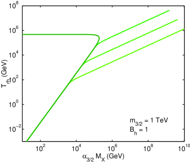
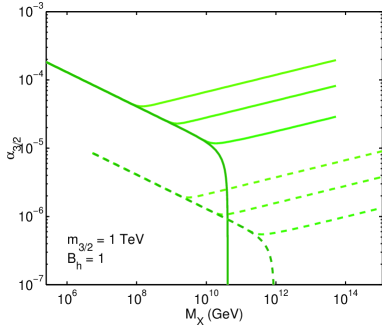
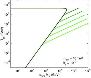
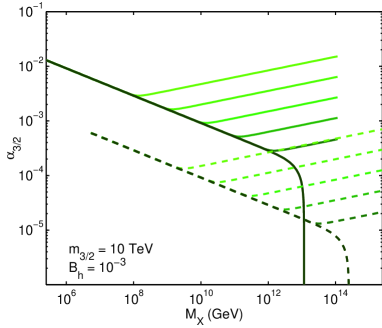
Figure 3: (Color online) Contours of constant $Y_{3/2}=Y_{3/2}^{BBN}$ for $M_{5}=10^{8},\,10^{9},\,10^{10},\,10^{11},\,10^{12},\,10^{13}$ GeV (from lighter to darker green). In the top panels we have $Y_{3/2}^{BBN}=4\times 10^{-17}$ ($m_{3/2}=1$ TeV and $B_{h}=1$), and in the bottom ones $Y_{3/2}^{BBN}=2\times 10^{-13}$ ($m_{3/2}=10$ TeV and $B_{h}=10^{-3}$). In the right panels we show two sets of curves for which we fixed $\alpha_{t}=1$ (full lines) and $\alpha_{t}=10^{-2}$ (dashed lines). For $m_{3/2}=1$ TeV, the $M_{5}\sim 10^{11}$ GeV curves already reproduce the results from SC, while for $m_{3/2}=10$ TeV we obtain the SC results only for $M_{5}\sim 10^{13}$ GeV.

In Fig. 3 we present the contours of constant $Y_{3/2}=Y_{3/2}^{BBN}$ for several values of $M_{5}$. We present the contours for $m_{3/2}=1$ TeV and $B_{h}=1$ (case I), for which $Y_{3/2}^{BBN}\lesssim 4\times 10^{-17}$, and $m_{3/2}=10$ TeV and $B_{h}=10^{-3}$ (case II), for which $Y_{3/2}^{BBN}\lesssim 2\times 10^{-13}$. In the right panels we show two sets of curves, one for $\alpha_{t}=1$ and the other for $\alpha_{t}=10^{-2}$. Once more we have fixed $m_{{\tilde{g}}}=1$ TeV in the computation of the thermal contribution to the gravitino abundance. Some of the curves are broken due to the upper limits on $T_{rh}$ and $M_{X}$ [cf. Eqs. (21) and (22), respectively] which come from $m_{3/2}>H$.

One should notice that for $m_{3/2}=1$ TeV, the curves corresponding to $M_{5}\gtrsim 10^{11}$ GeV already reproduce the results from SC, while for $m_{3/2}=10$ TeV we obtain the SC results only for $M_{5}\gtrsim 10^{13}$ GeV. The value of $M_{5}$ below which the BC effects affect the production of gravitinos can be easily obtained from Eq. (47). One has

$$M_{5}\lesssim 3.3\times 10^{10}\,{\rm GeV}~{},\quad{\rm for}~{}m_{3/2}=1~{}{\rm TeV}~{},$$ (58)

and

$$M_{5}\lesssim 9.7\times 10^{12}\,{\rm GeV}~{},\quad{\rm for}~{}m_{3/2}=10~{}{\rm TeV}~{}.$$ (59)

For 5D Planck masses above these values, the upper bounds on $T_{rh}$, $M_{X}$ and $\alpha_{3/2}$ derived for SC Asaka et al. (2006) are valid. For the reheating temperature one has [cf. Fig. 3 (left) and Eq. (41)]

$$T_{rh}\lesssim\left\{\begin{array}[]{l}4.7\times 10^{5}\,{\rm GeV}\quad{\rm(I)}~{},\\ 2.1\times 10^{9}\,{\rm GeV}\quad{\rm(II)}~{},\\ \end{array}\right.$$ (62)

while for the heavy scalar mass one finds [cf. Fig. 3 (right) and Eq. (42)]

$$M_{X}\lesssim\left\{\begin{array}[]{l}4.1\times 10^{10}\alpha_{t}^{-2/3}\,{\rm GeV}\quad{\rm(I)}~{},\\ 1.2\times 10^{13}\alpha_{t}^{-2/3}\,{\rm GeV}\quad{\rm(II)}~{},\\ \end{array}\right.$$ (65)

and for $\alpha_{3/2}$ [cf. Fig. 3 (right) and Eq. (43)]

$$\alpha_{3/2}\lesssim\left\{\begin{array}[]{l}1.3\times 10^{-5}\,\alpha_{t}^{1/2}\left(\dfrac{M_{X}}{10^{10}~{}{\rm GeV}}\right)^{-1/4}\quad{\rm(I)}~{},\\ 9.4\times 10^{-4}\,\alpha_{t}^{1/2}\left(\dfrac{M_{X}}{10^{10}~{}{\rm GeV}}\right)^{-1/4}\quad{\rm(II)}~{}.\\ \end{array}\right.$$ (68)

The lower bound on the reheating temperature presented in Eq. (49) reads in this case

$$T_{rh}\gtrsim\left\{\begin{array}[]{l}3.4\times 10^{4}\,{\rm GeV}\left(\dfrac{\alpha_{3/2}\,M_{X}}{10^{5}~{}{\rm GeV}}\right)^{2}\quad{\rm(I)}~{},\\ 6.8\,{\rm GeV}\left(\dfrac{\alpha_{3/2}\,M_{X}}{10^{5}~{}{\rm GeV}}\right)^{2}\quad{\rm(II)}~{}.\\ \end{array}\right.$$ (71)

For lower values of the 5D Planck mass, the disappearance of the upper bounds on $T_{rh}$ and $M_{X}$ coming from BBN limits on the amount of gravitinos will allow the Universe to reheat at a larger temperature and, at the same time, the scalar to have a larger mass and a larger decay rate into gravitinos than the ones allowed in SC. The upper bound in $M_{X}$ is simply the one given in Eq. (22), while the reheating temperature, in addition to $T_{rh}>T_{t}$, should satisfy

$$\left.\begin{array}[]{l}6.1\times 10^{4}\,{\rm GeV}\left(\dfrac{\alpha_{3/2}\,M_{X}}{10^{5}~{}{\rm GeV}}\right)^{2/3}\left(\dfrac{M_{5}}{10^{10}~{}{\rm GeV}}\right)\\ 3.5\times 10^{3}\,{\rm GeV}\left(\dfrac{\alpha_{3/2}\,M_{X}}{10^{5}~{}{\rm GeV}}\right)^{2/3}\left(\dfrac{M_{5}}{10^{10}~{}{\rm GeV}}\right)\\ \end{array}\right\}\lesssim T_{rh}\lesssim\left\{\begin{array}[]{l}4.2\times 10^{7}\,{\rm GeV}\left(\dfrac{M_{5}}{10^{10}~{}{\rm GeV}}\right)^{3/4}\quad{\rm(I)}~{},\\ 7.5\times 10^{7}\,{\rm GeV}\left(\dfrac{M_{5}}{10^{10}~{}{\rm GeV}}\right)^{3/4}\quad{\rm(II)}~{},\\ \end{array}\right.$$ (76)

obtained from Eqs. (48) and (19), respectively. In this regime, the upper bound on the coupling constant $\alpha_{3/2}$ will grow with $M_{X}$, in contrast with the SC scenario. From Eq. (50) we obtain

$$\alpha_{3/2}\lesssim\left\{\begin{array}[]{l}1.2\times 10^{-5}\,\alpha_{t}^{3/4}\left(\dfrac{M_{X}}{10^{10}~{}{\rm GeV}}\right)^{1/8}\left(\dfrac{M_{5}}{10^{10}~{}{\rm GeV}}\right)^{-3/8}\quad{\rm(I)}~{},\\ 8.4\times 10^{-4}\,\alpha_{t}^{3/4}\left(\dfrac{M_{X}}{10^{10}~{}{\rm GeV}}\right)^{1/8}\left(\dfrac{M_{5}}{10^{10}~{}{\rm GeV}}\right)^{-3/8}\quad{\rm(II)}~{}.\\ \end{array}\right.$$ (79)

Before concluding this section, it is worth commenting on the possible additional constraints coming from the LSP abundance, which is stable if R-parity is conserved. In this case one must impose that the abundance of LSP does not overclose the universe, as it contributes to the dark matter content. The LSP can be produced both from gravitino and heavy scalar decays. The LSP abundance from gravitino decays does not give additional bounds provided that $m_{3/2}=100~{}{\rm GeV}-10~{}{\rm TeV}$. The constraints coming from the production of the LSP from heavy scalar decays will be model dependent. In Ref. Asaka et al. (2006) the bounds arising from considering the neutral wino $\tilde{W}$ as the LSP, which maximizes the annihilation cross section and hence leads to the most conservative bounds, were derived in SC. In order to avoid the overclosure of the universe, a lower bound in $M_{X}$ is found, namely $M_{X}\gtrsim 2\times 10^{6}$ GeV for $M_{\tilde{W}}=100$ GeV, which becomes more stringent for larger wino masses. Since the brane effects are only present for heavy scalar masses $M_{X}\gtrsim\alpha_{t}^{-2/3}\,M_{5}$ [cf. Eq. (22)], one should expect that for sufficiently high values of $M_{5}$ these bounds will not change.

III.3 Stable gravitino and dark matter

In the case of a stable gravitino, when the gravitino is itself the LSP with exact R-parity, one should check whether the contribution of gravitinos to the energy density of the universe does not exceed the observed matter density limit. From the gravitino abundance, we can estimate their contribution to the closure density

$$\Omega_{3/2}h^{2}=m_{3/2}\,Y_{3/2}\,s_{0}\,h^{2}\rho_{c}^{-1}\,.$$ (80)

Here $\rho_{c}=3H_{0}^{2}M_{P}^{2}/8\pi=8.07\times 10^{-47}h^{2}$ GeV⁴ is the critical density and $s_{0}=2.22\times 10^{-38}$ GeV³ is the present entropy density. The total fraction of gravitinos contributing to dark matter, $\Omega_{3/2}$, is the sum of the two contributions

$$\Omega_{3/2}=\Omega_{3/2}^{X}+\Omega_{3/2}^{th}\,,$$ (81)

the first coming from the abundance of gravitinos due to the decay of the heavy scalar, Eq. (32), and the second from thermal production, Eq. (26). To avoid overclosure one must require

$$\Omega_{3/2}h^{2}\leq\Omega_{DM}h^{2}~{},$$ (82)

where we will use the WMAP bound on the matter density of the universe Bennett et al. (2003),

$$\Omega_{DM}h^{2}=0.143~{}.$$ (83)

If $\Omega_{3/2}=\Omega_{DM}$, the gravitinos constitute (all) the dark matter of the universe.

Let us now consider the two contributions to the gravitino dark matter. From the decay of the heavy scalar one has

$$\Omega_{3/2}^{X}h^{2} =2.8\times 10^{-2}\left(\dfrac{m_{3/2}}{10^{-1}\,{\rm GeV}}\right)\,\left(\dfrac{Y^{X}_{3/2}}{10^{-9}}\right)$$

$$=4.1\times 10^{-1}\,\left(\dfrac{B_{3/2}}{10^{-4}}\right)\,\left(\dfrac{m_{3/2}}{10^{-1}\,{\rm GeV}}\right)\,\left(\dfrac{M_{X}}{10^{10}\,{\rm GeV}}\right)^{-1}\,\left(\dfrac{T_{rh}}{10^{6}\,{\rm GeV}}\right)\,,$$ (84)

and from the thermal production

$$\Omega_{3/2}^{th}h^{2}=2.8\times 10^{-2}\left(\dfrac{m_{3/2}}{10^{-1}\,{\rm GeV}}\right)\,\left(\dfrac{Y^{th}_{3/2}}{10^{-9}}\right)\,.$$ (85)

In the SC case one can write

$$\Omega_{3/2}^{X}h^{2} =2.3\times 10^{-2}\,\alpha_{t}\,\left(\dfrac{B_{3/2}}{10^{-4}}\right)\,\left(\dfrac{m_{3/2}}{10^{-1}\,{\rm GeV}}\right)\,\left(\dfrac{M_{X}}{10^{10}\,{\rm GeV}}\right)^{1/2}\,,$$ (86)

$$\Omega_{3/2}^{th}h^{2} =1.6\times 10^{-2}\,\alpha_{t}\,\left[\dfrac{{\cal A}(T_{rh};m_{3/2},m_{{\tilde{g}}})}{10^{-14}~{}{\rm GeV}^{-1}}\right]\,\left(\dfrac{m_{3/2}}{10^{-1}\,{\rm GeV}}\right)\,\left(\dfrac{M_{X}}{10^{10}\,{\rm GeV}}\right)^{3/2}\,,$$ (87)

while in the BC regime one has

$$\Omega_{3/2}^{X}h^{2} =2.8\times 10^{-2}\,\alpha_{t}^{1/2}\,\left(\dfrac{B_{3/2}}{10^{-4}}\right)\,\left(\dfrac{m_{3/2}}{10^{-1}\,{\rm GeV}}\right)\,\left(\dfrac{M_{X}}{10^{10}\,{\rm GeV}}\right)^{-1/4}\,\left(\dfrac{M_{5}}{10^{10}\,{\rm GeV}}\right)^{3/4}\,,$$ (88)

$$\Omega_{3/2}^{th}h^{2} =4.4\times 10^{-2}\,\left[\dfrac{{\cal A}(T_{t};m_{3/2},m_{{\tilde{g}}})}{10^{-14}~{}{\rm GeV}^{-1}}\right]\,\left(\dfrac{m_{3/2}}{10^{-1}\,{\rm GeV}}\right)\,\left(\dfrac{M_{5}}{10^{10}\,{\rm GeV}}\right)^{3/2}\,.$$ (89)

Notice that, in both BC and SC, $\Omega_{3/2}^{X}h^{2}$ is proportional to $m_{3/2}$, while $\Omega_{3/2}^{th}h^{2}$ is inversely proportional to $m_{3/2}$, since ${\cal A}(T_{t};m_{3/2},m_{{\tilde{g}}})\sim m_{3/2}^{-2}$. This means that for large gravitino masses the $X$ decay contribution will dominate, while for small values of $m_{3/2}$, the main contribution comes from thermal production. On the other hand, the dependence of $\Omega_{3/2}^{X}h^{2}$ on $M_{X}$ is different in BC from that of SC. Once more, this implies that in the brane high-energy regime, there is no upper limit on the heavy scalar mass coming from the gravitino dark matter fraction.

One should notice that the momentum of the gravitinos produced by $X$ decay can be much larger than its mass since $p_{3/2}\simeq M_{X}/2$. Therefore, they can behave as warm dark matter and influence the structure formation: with a non negligible velocity, and before the time of matter-radiation equality, they can freely stream out of overdense regions and into underdense regions, and this can erase the small structures that are observed today. This leads to an upper bound on the present dispersion velocity of the gravitino $v_{3/2}^{0}$ Borgani et al. (1996); Jedamzik et al. (2006); Steffen (2006). The present velocity of dispersion of the gravitinos produced by the $X$ decay is estimated to be Jedamzik et al. (2006)

$$v_{3/2}^{0}\simeq\dfrac{1}{2}\dfrac{M_{X}}{m_{3/2}}\dfrac{T_{0}}{T_{rh}}\left(\dfrac{g_{*}(T_{0})}{g_{*}(T_{rh})}\right)^{1/3}~{},$$ (90)

where $T_{0}=2.35\times 10^{-13}$ GeV is the present photon temperature and $g_{*}(T_{0})=43/11$. Bounds on this velocity are obtained by means of the power spectrum inferred from Lyman-$\alpha$ together with cosmic microwave background radiation and galaxy clustering constraints Viel et al. (2005); Seljak et al. (2006). From Ref. Seljak et al. (2006) it was found Asaka et al. (2006) that $v_{3/2}^{0}\lesssim 4\times 10^{-8}$.

From the limit on the present velocity of dispersion one can estimate an approximate upper bound on the branching ratio of the decay channel into gravitinos $B_{3/2}$. Considering the contribution from the heavy scalar decay to the amount of gravitinos we can write

$$\Omega_{3/2}^{X}=\dfrac{3}{2}\,B_{3/2}\,\dfrac{m_{3/2}T_{rh}}{M_{X}}\,s_{0}\,\rho_{c}^{-1}\,,$$ (91)

from which

$$v_{3/2}^{0}=1.26\times 10^{-5}\dfrac{B_{3/2}}{\Omega_{3/2}^{X}h^{2}}~{}.$$ (92)

Assuming $\Omega_{3/2}^{X}h^{2}=\Omega_{DM}^{X}h^{2}$, one gets the approximate bound

$$B_{3/2}\lesssim 4.5\times 10^{-4}\,.$$ (93)

Notice that this bound is independent of the background cosmology. One can also compute the velocity of dispersion for gravitinos produced thermally, however one finds that for $m_{3/2}\gtrsim 100$ keV they have a negligible free-streaming behavior Steffen (2006). Here we will consider masses well above this bound. The above constraint in $B_{3/2}$ was determined assuming that all dark matter is constituted by gravitinos, $\Omega_{3/2}^{X}=\Omega_{DM}$. However, if gravitinos are only a fraction of dark matter, then the bound becomes weaker, and can even be evaded if

$$\Omega^{X}_{3/2}\lesssim 0.12\,\Omega_{DM}\,,$$ (94)

as derived in Ref. Viel et al. (2005).

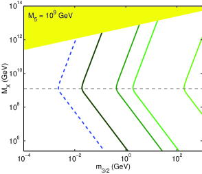
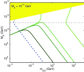
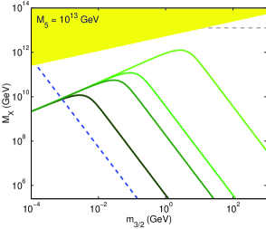
Figure 4: (Color online) Contour of constant $\Omega_{3/2}h^{2}=\Omega_{DM}h^{2}=0.143$ for $B_{3/2}=10^{-2},\,4.5\times 10^{-4},\,10^{-4},\,10^{-6}$ (darker to lighter, or left to right, green full lines) in the $M_{X}-m_{3/2}$ plane. The different panels correspond to various values of $M_{5}$. We have chosen $m_{{\tilde{g}}}=1$ TeV and $\alpha_{t}=1$. Also shown is the contour for $\Omega_{3/2}h^{2}=0.12\Omega_{DM}h^{2}$ (blue dashed line), when $B_{3/2}=10^{-2}$. The yellow shaded area is excluded because of the condition $H(T_{rh})<m_{3/2}$ [cf. Eq. (22)]. The horizontal line represents the value of $M_{X}$ for which the transition from the high to the low energy regime occurs.

In Fig. 4 we present the contours of constant $\Omega_{3/2}h^{2}=\Omega_{DM}h^{2},$ in the $M_{X}-m_{3/2}$ plane, with $\Omega_{DM}h^{2}$ given by the WMAP bound in Eq. (83). The different (green) full lines correspond to various values of $B_{3/2}$, where we fixed $\alpha_{t}=1$ and $m_{{\tilde{g}}}=1$ TeV. The allowed range of masses lies to the left and/or below the contour lines. Moreover the gravitino dark matter is only viable to the right/above the line which corresponds to the upper bound on the branching ratio shown in Eq. (93), $B_{3/2}=4.5\times 10^{-4}$. The yellow shaded area is excluded because of the condition $H(T_{rh})<m_{3/2}$ [cf. Eq. (22)]. The horizontal line represents the value of $M_{X}=\left(2/\alpha_{t}^{2}\right)^{1/3}M_{5}$, for which the transition from the high to the low energy regimes occurs. The contours are shown for three different values of the 5D Planck mass, namely, $M_{5}=10^{9},\,10^{11},\,10^{13}$ GeV.

In SC there is an upper limit on the mass of the heavy scalar $M_{X}$ coming from the bounds on the gravitino abundance. The maximum value of $M_{X}$ is obtained when both contributions to the gravitino production, from the heavy scalar decay and thermal scatterings, are equal; hence, at that point, one can write that the total abundance is $\Omega_{3/2}=2\sqrt{\Omega_{3/2}^{X}\,\Omega_{3/2}^{th}}<\Omega_{DM}$ and obtain

$$M_{X}\lesssim 7\times 10^{9}\,{\rm GeV}\,\alpha_{3/2}^{-1}\,.$$ (95)

We have taken into consideration that, for the gravitino mass in the range $10^{-4}-10^{2}$ GeV , ${\cal A}(T_{rh};m_{3/2},m_{{\tilde{g}}})\simeq 10^{-17}m_{3/2}^{-2}$ is a good approximation. As said before, in the high energy regime there is no such a bound, and the allowed values for $M_{X}$ are only constrained by the condition $H(T_{rh})<m_{3/2}$ [cf. Eq. (22)]. We see that, for low values of $M_{5}$ and a fixed $B_{3/2}$, it is possible to have larger values of both $M_{X}$ and $m_{3/2}$ and yet satisfy the bounds from dark matter. For example, for $M_{5}\sim 10^{9}$ GeV and sufficiently low branching ratio, it is possible to have $M_{X}\sim 10^{12}$ GeV while having $m_{3/2}\sim 100$ GeV.

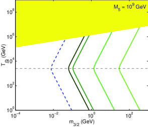
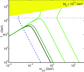
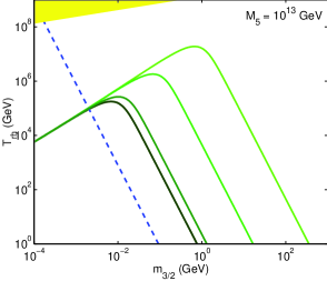
Figure 5: (Color online) Same as in Fig. 4, but in the $T_{rh}-m_{3/2}$ plane and for $\alpha_{3/2}B_{3/2}=10^{-3},\,4.5\times 10^{-4},\,10^{-5},\,10^{-7}$ (darker to lighter, or left to right, green full lines).

If one now takes $T_{rh}$ as the free parameter one can derive the contours of constant $\Omega_{3/2}h^{2}=\Omega_{DM}h^{2}$ in the $T_{rh}-m_{3/2}$, shown in Fig. 5 for different values of $M_{5}$. Here the different (green) full lines correspond to various values of $\alpha_{3/2}B_{3/2}$, and the gravitino dark matter is only viable to the right/above the line which corresponds to the upper bound on the branching ratio $B_{3/2}\lesssim 4.5\times 10^{-4}$ [since $\alpha_{3/2}\lesssim{\cal O}(1)$]. Once again one can distinguish the two behaviors for SC and high-energy BC regimes. The contributions to the gravitino dark matter read as

$$\Omega_{3/2}^{X}h^{2} =1.9\times 10^{-2}\,\left(\dfrac{\alpha_{3/2}B_{3/2}}{10^{-6}}\right)^{2/3}\left(\dfrac{m_{3/2}}{10^{-1}\,{\rm GeV}}\right)\,\left(\dfrac{T_{rh}}{10^{6}\,{\rm GeV}}\right)^{1/3}\,,$$ (96)

$$\Omega_{3/2}^{th}h^{2} =2.8\times 10^{-1}\,\left[\dfrac{{\cal A}(T_{t};m_{3/2},m_{{\tilde{g}}})}{10^{-14}~{}{\rm GeV}^{-1}}\right]\,\left(\dfrac{m_{3/2}}{10^{-1}\,{\rm GeV}}\right)\,\left(\dfrac{T_{rh}}{10^{6}\,{\rm GeV}}\right)\,,$$ (97)

in SC limit. In the BC regime we obtain

$$\Omega_{3/2}^{X}h^{2} =3.5\times 10^{-3}\,\left(\dfrac{\alpha_{3/2}\,B_{3/2}}{10^{-6}}\right)^{2/3}\left(\dfrac{m_{3/2}}{10^{-1}\,{\rm GeV}}\right)\left(\dfrac{T_{rh}}{10^{6}\,{\rm GeV}}\right)^{-1/3}\left(\dfrac{M_{5}}{10^{10}\,{\rm GeV}}\right)\,,$$ (98)

$$\Omega_{3/2}^{th}h^{2} =5.5\times 10^{-1}\,\left[\dfrac{{\cal A}(T_{t};m_{3/2},m_{{\tilde{g}}})}{10^{-14}~{}{\rm GeV}^{-1}}\right]\,\left(\dfrac{m_{3/2}}{10^{-1}\,{\rm GeV}}\right)\,\left(\dfrac{T_{t}}{10^{6}\,{\rm GeV}}\right)\,.$$ (99)

As expected, the bound

$$T_{rh}\lesssim 1.8\times 10^{6}\,{\rm GeV}\,\left(\dfrac{\alpha_{3/2}\,B_{3/2}}{10^{-5}}\right)^{1/2}\,,$$ (100)

derived for the SC case in order to avoid the overclosure of the universe by dark matter disappears when we consider sufficiently low 5D Planck scales $M_{5}$.

If $B_{3/2}>4.5\times 10^{-4}$, then the gravitinos can only contribute to a fraction of the total amount of dark matter. In Figs. 4 and 5 the blue-dashed line represents the contour for $\Omega_{3/2}h^{2}=0.12\Omega_{DM}h^{2}$, the maximum contribution of gravitinos (warm) dark matter that does not spoil the structure formation, for $B_{3/2}=10^{-2}$. We can see that in this case the bound becomes more stringent.

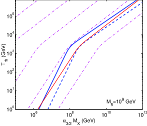
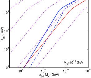
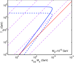
Figure 6: (Color online) Contours of constant $\Omega_{3/2}h^{2}=\Omega_{DM}h^{2}=0.143$ for $m_{3/2}=1$ GeV (full bold line) and $m_{3/2}=0.1$ GeV (dotted bold line) in the $T_{rh}-\alpha_{3/2}M_{X}$ plane. The dash-dotted lines represent the contours of constant $B_{3/2}=1,\,10^{-5},\,10^{-10},\,10^{-15},\,10^{-20}$ (from below to top), and the full line is the contour for $B_{3/2}=4.5\times 10^{-4}$. In the computation of the branching ratio we fixed $\alpha_{3/2}=1$. The different panels correspond to various values for $M_{5}$.

Finally, in Fig. 6 we show the contours of constant $\Omega_{3/2}h^{2}=\Omega_{DM}h^{2}$, in the $T_{rh}-\alpha_{3/2}M_{X}$ plane, for two different gravitino masses: $m_{3/2}=1,~{}0.1$ GeV (full and dotted bold lines, respectively) and $M_{5}=10^{9},10^{11},10^{13}$ GeV. Also shown are the contours of constant $B_{3/2}$ (dash-dotted lines) for a fixed $\alpha_{3/2}=1$. It is clearly seen from the figure that, in the BC regime and for sufficiently low values of $M_{5}$, higher reheating temperatures are allowed for large $M_{X}$.

IV Discussion and conclusion

We have studied the gravitino production in the braneworld cosmology context. Our framework is the RSII construction in which the Friedmann expansion law is modified with a quadratic term in the energy density. As an approximation, we considered the gravitino as a field localized on the UV brane and used 4D supersymmetry and the usual Boltzmann equation to describe its production.

In Figs. 7 and 8 we show the points, in the $T_{rh}-M_{X}$, $T_{rh}-M_{5}$ and $\alpha_{t}-\alpha_{3/2}$ planes, that satisfy the constraints discussed in detail in the other sections. We have allowed a variation of the couplings and masses in the ranges $10^{-8}\leq\alpha_{3/2}\leq 1$, $\,10^{-5}\leq\alpha_{t}\leq 1$, $\,10^{5}\,{\rm GeV}\leq M_{X}\leq 10^{15}\,{\rm GeV}$ and $10^{6}\,{\rm GeV}\leq M_{5}\leq 10^{16}\,{\rm GeV}$. For the stable gravitino case one has $10^{-4}\,{\rm GeV}\lesssim m_{3/2}\lesssim 10^{3}$ GeV. The light and dark green points correspond to the SC and BC high energy regimes, respectively.

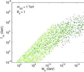
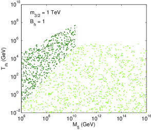
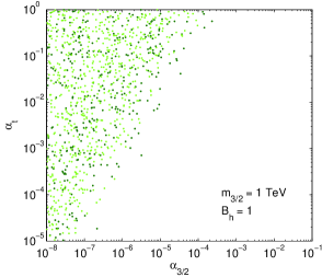
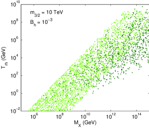
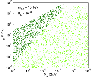
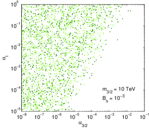
Figure 7: (Color online) Parameter space allowed by the gravitino abundance BBN bounds, in the $T_{rh}-M_{X}$, $T_{rh}-M_{5}$ and $\alpha_{t}-\alpha_{3/2}$ planes. In the top panels we have $Y_{3/2}^{BBN}=4\times 10^{-17}$ ($m_{3/2}=1$ TeV and $B_{h}=1$), and in the bottom one $Y_{3/2}^{BBN}=2\times 10^{-13}$ ($m_{3/2}=10$ TeV and $B_{h}=10^{-3}$). The light and dark green points correspond to the SC and BC high energy regimes, respectively.

For the unstable gravitino case, one can derive the range of $M_{5}$ for which the brane correction to the standard expansion rate is relevant. The upper bound for this range is dependent of the gravitino mass and we have obtained $M_{5}\lesssim 3.3\times 10^{10}$ GeV and $M_{5}\lesssim 9.7\times 10^{12}$ GeV, for $m_{3/2}=1,\,10$ TeV, respectively.

In the BC regime the upper bounds on the mass of the heavy scalar and the reheating temperature, coming from the gravitino abundance, disappear. Thus, with the inclusion of the brane correction, the parameter space with the correct gravitino abundance is enlarged. Both, larger reheating temperatures and larger masses for the heavy scalar are allowed. This is more evident for a smaller gravitino mass and a larger hadronic branching ratio. Although $T_{rh}$ and $M_{X}$ are not constrained by the gravitino abundance limits, they are bounded by the fact that $H>m_{3/2}$ for the gravitino decay to be possible.

On the other hand, in BC, like in SC, one also needs a small coupling $\alpha_{3/2}$ and/or a small branching ratio $B_{3/2}$. However, for a fixed $\alpha_{t}$, it is possible to have a slightly larger $\alpha_{3/2}$ in BC. The required lower value for $\alpha_{3/2}$ does not allow to solve the moduli problem by simply increasing the moduli mass, since, for the range of gravitino masses considered, $\alpha_{3/2}={\cal O}(1)$ is excluded. It also poses severe constraints to inflationary models. In order to achieve a small $\alpha_{3/2}$ one needs a VEV of $X$ (the inflaton in this case), much smaller than $M_{P}$; on the other hand, one can decrease $B_{3/2}$ if one increases $\alpha_{t}$, by demanding interactions of $X$ with the other MSSM particles with strength much larger than $M_{P}^{-1}$. A lower value for $\alpha_{3/2}$ can be achieved in some new and hybrid inflationary models, and in the simplest chaotic inflationary models, for which $G_{X}$ vanishes in the vacuum (see Refs. Asaka et al. (2006); Kawasaki et al. (2006b); Endo et al. (2006b)) one obtains $\alpha_{3/2}=0$ and then no gravitinos are produced in the decay of $X$.

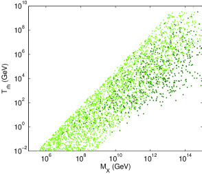
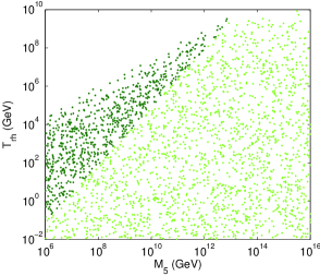
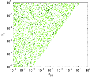
Figure 8: (Color online) Parameter space allowed by the dark matter bounds, $\Omega_{3/2}h^{2}\leq\Omega_{DM}h^{2}=0.143$, and $B_{3/2}\lesssim 4.5\times 10^{-4}$ , in the $T_{rh}-M_{X}$, $T_{rh}-M_{5}$ and $\alpha_{t}-\alpha_{3/2}$planes. The gravitino mass runs in the interval $10^{-4}-10^{3}$ GeV. The light and dark green points correspond to the SC and BC high energy regimes, respectively.

In the stable gravitino case, similar bounds can be derived. Notice however that the overclosure constraint alone allows to have $B_{3/2}\sim 10^{-2}$. Therefore, it would be possible to solve the moduli problem. But, if one takes into account the warm dark matter constraint, then one needs $B_{3/2}\lesssim 10^{-4}$, which means that $\alpha_{3/2}\lesssim 0.1\,\alpha_{t}$ (cf. Fig. 8). In Ref. Asaka et al. (2006) its was suggested that such a suppression in the coupling might be possible in some moduli stabilization mechanism. In that case it would be possible to have gravitino warm dark matter from the decay of a moduli field with mass as large as ${\cal O}(10^{11})-{\cal O}(10^{12})$ GeV, for a gravitino with $m_{3/2}\lesssim 3$ GeV and $M_{5}\sim{\cal O}(10^{9})$ (cf. Fig. 4). In SC, the upper bound for the mass of the moduli would be one order of magnitude bellow the BC one. Moreover, we should point out that the warm dark matter constraint disappears if the gravitino contributes with less than $12\%$ to the total dark matter density.

Finally, it would be interesting to further investigate the gravitino production in specific brane inflationary models. The gravitino production analysis presented here could also be extended to include the KK gravitino production process.