TUM-HEP-657/07

MPP-2007-17

Charged Lepton Flavour Violation and $\bm{(g-2)_{\mu}}$
in the Littlest Higgs Model with T-Parity:
a clear Distinction from Supersymmetry

Monika Blanke^a,b, Andrzej J. Buras^a, Björn Duling^a,
Anton Poschenrieder^a and Cecilia Tarantino^a

^aPhysik Department, Technische Universität München, D-85748 Garching, Germany

^bMax-Planck-Institut für Physik (Werner-Heisenberg-Institut),
D-80805 München, Germany

We calculate the rates for the charged lepton flavour violating decays $\ell_{i}\to\ell_{j}\gamma$, $\tau\to\ell\pi$, $\tau\to\ell\eta$, $\tau\to\ell\eta^{\prime}$, $\mu^{-}\to e^{-}e^{+}e^{-}$, the six three body leptonic decays $\tau^{-}\to\ell_{i}^{-}\ell_{j}^{+}\ell_{k}^{-}$ and the rate for $\mu-e$ conversion in nuclei in the Littlest Higgs model with T-Parity (LHT). We also calculate the rates for $K_{L,S}\to\mu e$, $K_{L,S}\to\pi^{0}\mu e$ and $B_{d,s}\to\ell_{i}\ell_{j}$. We find that the relative effects of mirror leptons in these transitions are by many orders of magnitude larger than analogous mirror quark effects in rare $K$ and $B$ decays analyzed recently. In particular, in order to suppress the $\mu\to e\gamma$ and $\mu^{-}\to e^{-}e^{+}e^{-}$ decay rates and the $\mu-e$ conversion rate below the experimental upper bounds, the relevant mixing matrix in the mirror lepton sector $V_{H\ell}$ must be rather hierarchical, unless the spectrum of mirror leptons is quasi-degenerate. We find that the pattern of the LFV branching ratios in the LHT model differs significantly from the one encountered in the MSSM, allowing in a transparent manner to distinguish these two models with the help of LFV processes. We also calculate $(g-2)_{\mu}$ and find the new contributions to $a_{\mu}$ below $1\cdot 10^{-10}$ and consequently negligible. We compare our results with those present in the literature.

Note added

An additional contribution to the $Z$ penguin in the Littlest Higgs model with T-parity has been pointed out in [1, 2], which has been overlooked in the present analysis. This contribution leads to the cancellation of the left-over quadratic divergence in the calculation of some rare decay amplitudes. Instead of presenting separate errata to the present work and our papers [3, 4, 5, 6] partially affected by this omission, we have presented a corrected and updated analysis of flavour changing neutral current processes in the Littlest Higgs model with T-parity in [7].

1 Introduction

Little Higgs models [8, 9, 10] offer an alternative route to the solution of the little hierarchy problem. One of the most attractive models of this class is the Littlest Higgs model with T-parity (LHT) [11], where the discrete symmetry forbids tree-level corrections to electroweak observables, thus weakening the electroweak precision constraints [12]. In this model, the new gauge bosons, fermions and scalars are sufficiently light to be discovered at LHC and there is a dark matter candidate [13]. Moreover, the flavour structure of the LHT model is richer than the one of the Standard Model (SM), mainly due to the presence of three doublets of mirror quarks and three doublets of mirror leptons and their weak interactions with the ordinary quarks and leptons.

Recently, in two detailed analyses, we have investigated in the LHT model $\Delta F=2$ [14] and $\Delta F=1$ [3] flavour changing neutral current (FCNC) processes, like particle-antiparticle mixings, $B\to X_{s}\gamma$, $B\to X_{s}\ell^{+}\ell^{-}$ and rare $K$ and $B$ decays. The first analysis of particle-antiparticle mixing in this model was presented in [15] and the FCNC processes in the LH model without T-parity have been presented in [17, 18, 19, 16, 20].

The most relevant messages of the phenomenological analyses in [14, 3, 17, 20] are:

• In the LH model without T-parity, which belongs to the class of models with constrained minimal flavour violation (CMFV) [21, 22], the new physics (NP) effects are small as the NP scale $f$ is required to be above $2-3\,{\rm TeV}$ in order to satisfy the electroweak precision constraints.

• In the LHT model, which is not stringently constrained by the latter precision tests and contains new flavour and CP-violating interactions, large departures from the SM predictions are found, in particular for CP-violating observables that are strongly suppressed in the SM. These are first of all the branching ratio for $K_{L}\rightarrow\pi^{0}\nu\bar{\nu}$ and the CP asymmetry $S_{\psi\phi}$ in the $B_{s}\to\psi\phi$ decay, but also $Br(K_{L}\to\pi^{0}\ell^{+}\ell^{-})$ and $Br(K^{+}\to\pi^{+}\nu\bar{\nu})$. Smaller, but still significant, effects have been found in rare $B_{s,d}$ decays and $\Delta M_{s,d}$.

• The presence of left-over divergences in $\Delta F=1$ processes, that signals some sensitivity to the ultraviolet (UV) completion of the theory, introduces some theoretical uncertainty in the evaluation of the relevant branching ratios both in the LH model [20] and the LHT model [3]. On the other hand, $\Delta F=2$ processes and the $B\to X_{s}\gamma$ decay are free from these divergences.

Now, it is well known that in the SM the FCNC processes in the lepton sector, like $\ell_{i}\to\ell_{j}\gamma$ and $\mu^{-}\to e^{-}e^{+}e^{-}$, are very strongly suppressed due to tiny neutrino masses. In particular, the branching ratio for $\mu\to e\gamma$ in the SM amounts to at most $10^{-54}$, to be compared with the present experimental upper bound, $1.2\cdot 10^{-11}$ [23], and with the one that will be available within the next two years, $\sim 10^{-13}$ [24]. Results close to the SM predictions are expected within the LH model without T-parity, where the lepton sector is identical to the one of the SM and the additional ${\cal O}(v^{2}/f^{2})$ corrections have only minor impact on this result. Similarly the new effects on $(g-2)_{\mu}$ turn out to be small [25].

A very different situation is to be expected in the LHT model, where the presence of new flavour violating interactions and of mirror leptons with masses of order $1\,{\rm TeV}$ can change the SM expectations up to 45 orders of magnitude, bringing the relevant branching ratios for lepton flavour violating (LFV) processes close to the bounds available presently or in the near future. Indeed in two recent interesting papers [26, 27], it has been pointed out that very large enhancements of the branching ratios for $\ell_{i}\to\ell_{j}\gamma$ and $\tau\to\mu\pi$ are possible within the LHT model.

The main goal of our paper is a new analysis of $\ell_{i}\to\ell_{j}\gamma$, $\tau\to\mu\pi$, and of other LFV processes not considered in [26, 27], with the aim to find the pattern of LFV in this model and to constrain the mass spectrum of mirror leptons and the new weak mixing matrix in the lepton sector $V_{H\ell}$, that in addition to three mixing angles contains three CP-violating phases. In particular we have calculated the rates for $\mu^{-}\to e^{-}e^{+}e^{-}$ and the six three body leptonic $\tau$ decays $\tau^{-}\to\ell_{i}^{-}\ell_{j}^{+}\ell_{k}^{-}$, as well as the $\mu-e$ conversion rate in nuclei. We have also calculated the rates for $K_{L,S}\to\mu e$, $K_{L,S}\to\pi^{0}\mu e$ and $B_{d,s}\to\ell_{i}\ell_{j}$ that are sensitive to flavour violation both in the mirror quark and mirror lepton sectors. Finally we calculated $(g-2)_{\mu}$ that has also been considered in [26, 27].

Our analysis confirms the findings of [26, 27] at the qualitative level: the impact of mirror leptons on the charged LFV processes $\ell_{i}\to\ell_{j}\gamma$ and $\tau\to\mu\pi$ can be spectacular while the impact on $(g-2)_{\mu}$ is small, although our analytical expressions differ from the ones presented in [26, 27]. Moreover, our numerical analysis includes also other LFV processes, not considered in [26, 27], where very large effects turn out to be possible.

While the fact that in the LHT model several LFV branching ratios can reach their present experimental upper bounds is certainly interesting, it depends sensitively on the parameters of the model. One of the most important results of the present paper is the identification of correlations between various branching ratios that on the one hand are less parameter dependent and on the other hand, and more importantly, differ significantly from corresponding correlations in the Minimal Supersymmetric Standard Model (MSSM) discussed in [29, 30, 31, 32]. The origin of this difference is that the dominance of the dipole operators in the decays in question present in the MSSM is replaced in the LHT model by the dominance of $Z^{0}$-penguin and box diagram contributions with the dipole operators playing now a negligible role. As a consequence, LFV processes can help to distinguish these two models.

A detailed analysis of LFV in the LHT model is also motivated by the prospects in the measurements of LFV processes with much higher sensitivity than presently available. In particular the MEG experiment at PSI [24] should be able to test $Br(\mu\to e\gamma)$ at the level of ${\cal O}(10^{-13}-10^{-14})$, and the Super Flavour Factory [33] is planned to reach a sensitivity for $Br(\tau\to\mu\gamma)$ of at least ${\cal O}(10^{-9})$. The planned accuracy of SuperKEKB of ${\cal O}(10^{-8})$ for $\tau\to\mu\gamma$ is also of great interest. Very important will also be an improved upper bound on $\mu-e$ conversion in Ti. In this context the dedicated J-PARC experiment PRISM/PRIME [34] should reach the sensitivity of ${\cal O}(10^{-18})$, i. e. an improvement by six orders of magnitude relative to the present upper bound from SINDRUM II at PSI [35].

Our paper is organized as follows. In Section 2 we briefly summarize those ingredients of the LHT model that are of relevance for our analysis. Section 3 is devoted to the decays $\ell_{i}\to\ell_{j}\gamma$ with particular attention to $\mu\to e\gamma$, for which a new stringent experimental upper bound should be available in the coming years. In Section 4 we calculate the branching ratio for $\tau\to\mu\pi$ and other semi-leptonic $\tau$ decays for which improved upper bounds are available from Belle. In Section 5 we analyze the decays $\mu^{-}\to e^{-}e^{+}e^{-}$, $\tau^{-}\to\mu^{-}\mu^{+}\mu^{-}$ and $\tau^{-}\to e^{-}e^{+}e^{-}$. In Section 6 we calculate the $\mu-e$ conversion rate in nuclei, and in Section 7 the decays $K_{L,S}\to\mu e$ and $K_{L,S}\to\pi^{0}\mu e$. In Section 8 we give the results for $B_{d,s}\to\mu e,\,\tau e,\,\tau\mu$ and in Sections 9 and 10 for $\tau^{-}\to e^{-}\mu^{+}e^{-},\,\mu^{-}e^{+}\mu^{-},\,\mu^{-}e^{+}e^{-},\,e^{-}\mu^{+}\mu^{-}$. In Section 11 we calculate $(g-2)_{\mu}$. A detailed numerical analysis of all these processes is presented in Section 12. In Section 13 we analyze various correlations between LFV branching ratios and compare them with the MSSM results in [29, 30, 31, 32]. Finally, in Section 14 we conclude our paper with a list of messages from our analysis and with a brief outlook. Few technical details are relegated to the appendices.

2 The LHT Model and its Lepton Sector

A detailed description of the LHT model and the relevant Feynman rules can be found in [3]. Here we just want to state briefly the ingredients needed for the present analysis.

2.1 Gauge Boson Sector

The T-even electroweak gauge boson sector consists only of the SM electroweak gauge bosons $W^{\pm}_{L}$, $Z_{L}$ and $A_{L}$.

The T-odd gauge boson sector consists of three heavy “partners” of the SM gauge bosons

$$W_{H}^{\pm}\,,\qquad Z_{H}\,,\qquad A_{H}\,,$$ (2.1)

with masses given to lowest order in $v/f$ by

$$M_{W_{H}}=gf\,,\qquad M_{Z_{H}}=gf\,,\qquad M_{A_{H}}=\frac{g^{\prime}f}{\sqrt{5}}\,.$$ (2.2)

All three gauge bosons will be present in our analysis. Note that

$$M_{A_{H}}=\frac{\tan{\theta_{W}}}{\sqrt{5}}M_{W_{H}}\simeq\frac{M_{W_{H}}}{4.1}\,,$$ (2.3)

where $\theta_{W}$ is the weak mixing angle.

2.2 Fermion Sector

The T-even sector of the LHT model contains just the SM fermions and the heavy top partner $T_{+}$. Due to the smallness of neutrino masses, the T-even contributions to LFV processes can be neglected with respect to the T-odd sector. We comment on the issue of neutrino masses in the LHT model in Appendix A.

The T-odd fermion sector [36] consists of three generations of mirror quarks and leptons with vectorial couplings under $SU(2)_{L}\times U(1)_{Y}$. In this paper, except for $K_{L,S}\to\mu e$, $K_{L,S}\to\pi^{0}\mu e$, $B_{d,s}\to\ell_{i}\ell_{j}$ and $\tau\to\ell\pi,\ell\eta,\ell\eta^{\prime}$, only mirror leptons are relevant. We will denote them by

$$\begin{pmatrix}\nu^{1}_{H}\\ \ell^{1}_{H}\end{pmatrix}\,,\qquad\begin{pmatrix}\nu^{2}_{H}\\ \ell^{2}_{H}\end{pmatrix}\,,\qquad\begin{pmatrix}\nu^{3}_{H}\\ \ell^{3}_{H}\end{pmatrix}\,,$$ (2.4)

with their masses satisfying to first order in $v/f$

$$m^{\nu}_{H1}=m^{\ell}_{H1}\,,\qquad m^{\nu}_{H2}=m^{\ell}_{H2}\,,\qquad m^{\nu}_{H3}=m^{\ell}_{H3}\,.$$ (2.5)

2.3 Weak Mixing in the Mirror Lepton Sector

As discussed in detail in [15], one of the important ingredients of the mirror sector is the existence of four CKM-like [37] unitary mixing matrices, two for mirror quarks and two for mirror leptons:

$$V_{Hu}\,,\quad V_{Hd}\,,\qquad V_{H\ell}\,,\quad V_{H\nu}\,.$$ (2.6)

They satisfy

$$V_{Hu}^{\dagger}V_{Hd}=V_{\text{CKM}}\,,\qquad V_{H\nu}^{\dagger}V_{H\ell}=V_{\text{PMNS}}^{\dagger}\,,$$ (2.7)

where in $V_{\text{PMNS}}$ [38] the Majorana phases are set to zero as no Majorana mass term has been introduced for right-handed neutrinos. The mirror mixing matrices in (2.6) parameterize flavour violating interactions between SM fermions and mirror fermions that are mediated by the heavy gauge bosons $W_{H}^{\pm}$, $Z_{H}$ and $A_{H}$. The notation in (2.6) indicates which of the light fermions of a given electric charge participates in the interaction.

Thus $V_{H\ell}$, the most important mixing matrix in the present paper, parameterizes the interactions of light charged leptons with mirror neutrinos, mediated by $W_{H}^{\pm}$, and with mirror charged leptons, mediated by $Z_{H}$ and $A_{H}$. Feynman rules for these interactions can be found in [3]. $V_{H\nu}$ parameterizes, on the other hand, the interactions of light neutrinos with mirror leptons.

In the course of our analysis of charged LFV decays it will be useful to introduce the following quantities ($i=1,2,3$):

$$\chi_{i}^{(\mu e)}=V^{*ie}_{H\ell}V^{i\mu}_{H\ell}\,,\qquad\chi_{i}^{(\tau e)}=V^{*ie}_{H\ell}V^{i\tau}_{H\ell}\,,\qquad\chi_{i}^{(\tau\mu)}=V^{*i\mu}_{H\ell}V^{i\tau}_{H\ell}\,,$$ (2.8)

that govern $\mu\to e$, $\tau\to e$ and $\tau\to\mu$ transitions, respectively.

We also recall the analogous quantities in the mirror quark sector $(i=1,2,3)$

$$\xi_{i}^{(K)}=V^{*is}_{Hd}V^{id}_{Hd}\,,\qquad\xi_{i}^{(d)}=V^{*ib}_{Hd}V^{id}_{Hd}\,,\qquad\xi_{i}^{(s)}=V^{*ib}_{Hd}V^{is}_{Hd}\,,$$ (2.9)

that we will need for the analysis of the decays $K_{L,S}\to\mu e$, $K_{L,S}\to\pi^{0}\mu e$ and $B_{d,s}\to\ell_{i}\ell_{j}$.

Following [28], we parameterize $V_{H\ell}$ in terms of three mixing angles $\theta_{ij}^{\ell}$ and three complex phases $\delta_{ij}^{\ell}$ as a product of three rotations, and introducing a complex phase in each of them, thus obtaining

$$V_{H\ell}=\begin{pmatrix}1&0&0\\ 0&c_{23}^{\ell}&s_{23}^{\ell}e^{-i\delta^{\ell}_{23}}\\ 0&-s_{23}^{\ell}e^{i\delta^{\ell}_{23}}&c_{23}^{\ell}\\ \end{pmatrix}\,\cdot\begin{pmatrix}c_{13}^{\ell}&0&s_{13}^{\ell}e^{-i\delta^{\ell}_{13}}\\ 0&1&0\\ -s_{13}^{\ell}e^{i\delta^{\ell}_{13}}&0&c_{13}^{\ell}\\ \end{pmatrix}\,\cdot\begin{pmatrix}c_{12}^{\ell}&s_{12}^{\ell}e^{-i\delta^{\ell}_{12}}&0\\ -s_{12}^{\ell}e^{i\delta^{\ell}_{12}}&c_{12}^{\ell}&0\\ 0&0&1\\ \end{pmatrix}$$ (2.10)

Performing the product one obtains the expression

$$V_{H\ell}=\begin{pmatrix}c_{12}^{\ell}c_{13}^{\ell}&s_{12}^{\ell}c_{13}^{\ell}e^{-i\delta^{\ell}_{12}}&s_{13}^{\ell}e^{-i\delta^{\ell}_{13}}\\ -s_{12}^{\ell}c_{23}^{\ell}e^{i\delta^{\ell}_{12}}-c_{12}^{\ell}s_{23}^{\ell}s_{13}^{\ell}e^{i(\delta^{\ell}_{13}-\delta^{\ell}_{23})}&c_{12}^{\ell}c_{23}^{\ell}-s_{12}^{\ell}s_{23}^{\ell}s_{13}^{\ell}e^{i(\delta^{\ell}_{13}-\delta^{\ell}_{12}-\delta^{\ell}_{23})}&s_{23}^{\ell}c_{13}^{\ell}e^{-i\delta^{\ell}_{23}}\\ s_{12}^{\ell}s_{23}^{\ell}e^{i(\delta^{\ell}_{12}+\delta^{\ell}_{23})}-c_{12}^{\ell}c_{23}^{\ell}s_{13}^{\ell}e^{i\delta^{\ell}_{13}}&-c_{12}^{\ell}s_{23}^{\ell}e^{i\delta^{\ell}_{23}}-s_{12}^{\ell}c_{23}^{\ell}s_{13}^{\ell}e^{i(\delta^{\ell}_{13}-\delta^{\ell}_{12})}&c_{23}^{\ell}c_{13}^{\ell}\\ \end{pmatrix}$$ (2.11)

As in the case of the CKM matrix the angles $\theta_{ij}^{\ell}$ can all be made to lie in the first quadrant with $0\leq\delta^{\ell}_{12},\delta^{\ell}_{23},\delta^{\ell}_{13}<2\pi$. The matrix $V_{H\nu}$ is then determined through $V_{H\nu}=V_{H\ell}V_{\text{PMNS}}$.

2.4 The Parameters of the LHT Model

The new parameters of the LHT model, relevant for the present study, are

$$f\,,\quad m^{\ell}_{H1}\,,\quad m^{\ell}_{H2}\,,\quad m^{\ell}_{H3}\,,\quad\theta_{12}^{\ell}\,,\quad\theta_{13}^{\ell}\,,\quad\theta_{23}^{\ell}\,,\quad\delta_{12}^{\ell}\,\quad\delta_{13}^{\ell}\,\quad\delta_{23}^{\ell}\,,$$ (2.12)

and the ones in the mirror quark sector that can be probed by FCNC processes in $K$ and $B$ meson systems, as discussed in detail in [14, 3].

The determination of the parameters in (2.12) with the help of LFV processes is clearly a formidable task. However, if the new particles present in the LHT model are discovered once LHC starts its operation, the parameter $f$ will be determined from $M_{W_{H}}$, $M_{Z_{H}}$ or $M_{A_{H}}$. Similarly the mirror lepton masses $m^{\ell}_{Hi}$ will be measured.

The only remaining free parameters among the ones listed in (2.12) will then be $\theta_{ij}^{\ell}$ and $\delta_{ij}^{\ell}$, which can be determined once many LFV processes have been measured.

3 $\ell_{i}\to\ell_{j}\gamma$ in the LHT Model

3.1 Preliminaries

In [14] we have shown how one can obtain the branching ratio $Br(B\to X_{s}\gamma)$ in the LHT model directly from the $B\to X_{s}\gamma$ and $b\to s\,\text{gluon}$ decays in the SM by simply changing the arguments of the two SM functions $D^{\prime}_{0}(x)$ and $E^{\prime}_{0}(x)$ and adjusting properly various overall factors. The explicit formulae for these functions are given in Appendix B.

Here we will proceed in an analogous way. We will first derive $Br(\mu\to e\gamma)$ in the SM for arbitrary neutrino masses from the calculation of $Br(B\to X_{s}\gamma)$ in the same model. This will allow us to obtain in a straightforward manner $Br(\mu\to e\gamma)$ in the LHT model, when also some elements of the $Br(B\to X_{s}\gamma)$ calculation in this model in [14] are taken into account. The generalization to $\tau\to\mu\gamma$ and $\tau\to e\gamma$ will be automatic.

The current experimental upper bounds for $\mu\to e\gamma$, $\tau\to\mu\gamma$ and $\tau\to e\gamma$ are given by [23, 39]

$$Br(\mu\to e\gamma)<1.2\cdot 10^{-11}\,,$$ (3.1)

$${Br(\tau\to\mu\gamma)<1.6\cdot 10^{-8}\,,\qquad Br(\tau\to e\gamma)<9.4\cdot 10^{-8}\,.}$$ (3.2)

3.2 $\mu\to e\gamma$ in the SM

The diagrams for the $B\to X_{s}\gamma$ and $\mu\to e\gamma$ decays in the SM are shown in Figs. 1 and 2, respectively. In $R_{\xi}$ gauge also the corresponding diagrams with Goldstone bosons contribute. The diagram with the photon coupled directly to the internal fermion line, present in $B\to X_{s}\gamma$, is absent in the case of $\mu\to e\gamma$ due to the neutrino charge neutrality.

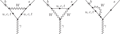
Figure 1: Diagrams contributing to $B\to X_{s}\gamma$ in the SM.

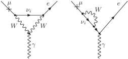
Figure 2: Diagrams contributing to $\mu\to e\gamma$ in the SM.

In the case of the $B\to X_{s}\gamma$ decay the function $D^{\prime}_{0}(x)$ resulting from the diagrams in Fig. 1 can be decomposed as follows

$$D^{\prime}_{0}(x)=\left[D^{\prime}_{0}(x)\right]_{\text{Abelian}}+\left[D^{\prime}_{0}(x)\right]_{\text{triple}}\,,$$ (3.3)

where the first term on the r. h. s. represents the sum of the first and the last diagram in Fig. 1 and the second term the second diagram.

The inspection of an explicit calculation of the $b\to s\gamma$ transition in the ’t Hooft-Feynman gauge gives

$$\left[D^{\prime}_{0}(x)\right]_{\text{Abelian}}=(2Q_{d}-Q_{u})E^{\prime}_{0}(x)\,,$$ (3.4)

with $Q_{d}$ and $Q_{u}$ being the electric charges of external and internal fermions, respectively. Setting $Q_{d}=-1/3$ and $Q_{u}=2/3$ in (3.4) and using (3.3) we find

$$\left[D^{\prime}_{0}(x)\right]_{\text{triple}}=D^{\prime}_{0}(x)+\frac{4}{3}E^{\prime}_{0}(x)\,.$$ (3.5)

This contribution is independent of fermion electric charges and can be directly used in the $\mu\to e\gamma$ decay.

Turning now our attention to the latter decay we find first from (3.4)

$$\left[D^{\prime}_{0}(x)\right]_{\text{Abelian}}^{\mu\to e\gamma}=-2E^{\prime}_{0}(x)\,,$$ (3.6)

as $Q_{u}=0$ and $Q_{d}=-1$ in this case. The final result for the relevant short distance function in the case of $\mu\to e\gamma$ is then given by the sum of (3.5) and (3.6). Denoting this function by $H(x_{\nu}^{i})$ we find

$$H(x_{\nu}^{i})=D^{\prime}_{0}(x_{\nu}^{i})-\frac{2}{3}E^{\prime}_{0}(x_{\nu}^{i})\,,\qquad x_{\nu}^{i}=\left(\frac{m^{i}_{\nu}}{M_{W}}\right)^{2}\,.$$ (3.7)

The generalization of the known SM result to arbitrary neutrino masses reads then

$$Br(\mu\to e\gamma)_{\text{SM}}=\frac{3\alpha}{2\pi}\left|\sum_{i}V_{ei}V^{*}_{\mu i}H(x_{\nu}^{i})\right|^{2}\,,$$ (3.8)

with $V_{ij}$ being the elements of the PMNS matrix.

Now, in the limit of small neutrino masses,

$$H(x_{\nu}^{i}){\longrightarrow}\frac{x^{i}_{\nu}}{4}\qquad\text{as}\quad{x^{i}_{\nu}\rightarrow 0}\,,$$ (3.9)

and we confirm the known result

$$Br(\mu\to e\gamma)_{\text{SM}}=\frac{3\alpha}{32\pi}\left|\sum_{i}V_{ei}V^{*}_{\mu i}x_{\nu}^{i}\right|^{2}\,.$$ (3.10)

Assuming that the angle $\theta_{13}$ of the PMNS matrix is not very small so that $\Delta m_{\text{atm}}^{2}$ dominates the branching ratio, we find

$$Br(\mu\to e\gamma)_{\text{SM}}\simeq 0.015\,\alpha\,s_{13}^{2}\left[\frac{\Delta m_{\text{atm}}^{2}}{M_{W}^{2}}\right]^{2}<10^{-54}\,,$$ (3.11)

where $\Delta m^{2}_{\text{atm}}\mathrel{\hbox to0.0pt{\raise 2.20013pt\hbox{$<$}\hss}{\lower 2.20013pt\hbox{$\sim$}}}3.2\cdot 10^{-3}\,\text{eV}^{2}$ and $s_{13}<0.2$ [42].

3.3 $\mu\to e\gamma$ in the LHT Model

The diagrams contributing to $\mu\to e\gamma$ in the LHT model are shown in Fig. 3. We show only the contributions from the mirror fermion sector as the T-even sector gives a negligible contribution. Note that the heavy scalar triplet $\Phi$ does not contribute at this order in $v/f$ (see [14, 3] for details).

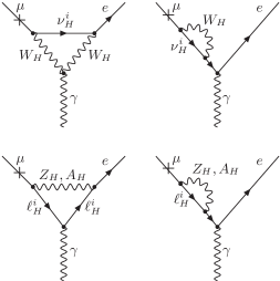
Figure 3: Diagrams contributing to $\mu\to e\gamma$ in the LHT model.

Let us write the resulting branching ratio as follows

$$Br(\mu\to e\gamma)_{\text{LHT}}=\frac{3\alpha}{2\pi}\left|\Delta_{W_{H}}+\Delta_{Z_{H}}+\Delta_{A_{H}}\right|^{2}\,,$$ (3.12)

with the different terms representing the $W_{H}^{\pm}$, $Z_{H}$ and $A_{H}$ contributions.

Defining

$$y_{i}=\frac{{m^{\ell}_{Hi}}^{2}}{M_{W_{H}}^{2}}\,,\qquad y_{i}^{\prime}=a\,y_{i}\quad\text{with }\;a=\frac{5}{\tan^{2}\theta_{W}}\simeq 16.6\,,$$ (3.13)

and including the factor

$$\frac{M_{W_{L}}^{2}}{M_{W_{H}}^{2}}=\frac{1}{4}\frac{v^{2}}{f^{2}}\,,$$ (3.14)

we find, using (3.8),

$$\Delta_{W_{H}}=\frac{1}{4}\frac{v^{2}}{f^{2}}\sum_{i}\chi_{i}^{(\mu e)}H(y_{i})\,,$$ (3.15)

with $H$ defined in (3.7) and $\chi_{i}^{(\mu e)}$ in (2.8).

The neutral gauge boson contributions can directly be deduced from (4.10) of [14]. Including a factor 3 that takes into account the difference between the electric charges of quarks and leptons, we obtain from the last two terms in (4.10) of [14]

$$\Delta_{Z_{H}} = \frac{1}{4}\frac{v^{2}}{f^{2}}\sum_{i}\chi_{i}^{(\mu e)}\left[-\frac{1}{2}E^{\prime}_{0}(y_{i})\right],$$ (3.16)

$$\Delta_{A_{H}} = \frac{1}{4}\frac{v^{2}}{f^{2}}\sum_{i}\chi_{i}^{(\mu e)}\left[-\frac{1}{10}E^{\prime}_{0}(y^{\prime}_{i})\right].$$ (3.17)

Finally, adding the three contributions in (3.15)–(3.17), we find using (3.12)

$$Br(\mu\to e\gamma)_{\text{LHT}}=\frac{3\alpha}{2\pi}\left|\bar{D}^{\prime\,\mu e}_{\text{odd}}\right|^{2}\,,$$ (3.18)

with

$$\bar{D}^{\prime\,\mu e}_{\text{odd}}=\frac{1}{4}\frac{v^{2}}{f^{2}}\left[\sum_{i}\chi_{i}^{(\mu e)}\left(D^{\prime}_{0}(y_{i})-\frac{7}{6}E^{\prime}_{0}(y_{i})-\frac{1}{10}E^{\prime}_{0}(y^{\prime}_{i})\right)\right]\,,$$ (3.19)

with $\chi_{i}^{(\mu e)}$ defined in (2.8), $y_{i}$ in (3.13) and $D^{\prime}_{0}$, $E^{\prime}_{0}$ given in Appendix B. The formulae (3.18) and (3.19) represent the main result of this section.

Let us next compare our result with the one of Goyal [26], which has been obtained without including the interferences between $\Delta_{W_{H}}$, $\Delta_{Z_{H}}$ and $\Delta_{A_{H}}$, whose omission cannot be justified. His results for $|\Delta_{W_{H}}|^{2}$, $|\Delta_{Z_{H}}|^{2}$ and $|\Delta_{A_{H}}|^{2}$ agree with ours, provided the latter contribution is divided by 25 in (15) of [26], once one assumes the straightforward relation $F_{A_{H}}(Z_{A_{H}})=F_{Z_{H}}(aZ_{Z_{H}})$ between the $A_{H}$ and $Z_{H}$ short distance functions. Note that the short distance functions $F_{j}(z_{i})$ in [26] still contain mass independent terms that disappear in the final expressions after the unitarity of the $V_{H\ell}$ matrix has been used. For this reason we have removed such terms from the functions $D^{\prime}_{0}(x)$ and $E^{\prime}_{0}(x)$. Finally, in contrast to [26], we find that the contributions of the scalar triplet $\Phi$ are of higher order in $v/f$.

In a recent paper by Choudhury et al. [27] a new analysis of $\ell_{i}\to\ell_{j}\gamma$ has been presented in which the interference terms have been taken into account. Unfortunately, the formulae in that paper are quite complicated thus preventing us from making an analytic comparison. On the other hand, we have performed a numerical comparison, finding significant differences between our results and those in [27].

3.4 $\tau\to e\gamma$ and $\tau\to\mu\gamma$ in the LHT Model

The branching ratios for $\tau\to e\gamma$ and $\tau\to\mu\gamma$ can easily be found in analogy to $\mu\to e\gamma$. We find

$$Br(\tau\to e\gamma) = \frac{3\alpha}{2\pi}Br(\tau^{-}\to\nu_{\tau}e^{-}\bar{\nu}_{e})\left|\bar{D}^{\prime\,\tau e}_{\text{odd}}\right|^{2}\,,$$ (3.20)

$$Br(\tau\to\mu\gamma) = \frac{3\alpha}{2\pi}Br(\tau^{-}\to\nu_{\tau}\mu^{-}\bar{\nu}_{\mu})\left|\bar{D}^{\prime\,\tau\mu}_{\text{odd}}\right|^{2}\,,$$ (3.21)

where $\bar{D}^{\prime\,\tau e}_{\text{odd}}$ and $\bar{D}^{\prime\,\tau\mu}_{\text{odd}}$ can be obtained from (3.19) by replacing $(\mu e)$ with $(\tau e)$ and $(\tau\mu)$, respectively. Furthermore [43]

$$Br(\tau^{-}\to\nu_{\tau}e^{-}\bar{\nu}_{e})=(17.84\pm 0.05)\%\,,\qquad Br(\tau^{-}\to\nu_{\tau}\mu^{-}\bar{\nu}_{\mu})=(17.36\pm 0.05)\%\,.$$ (3.22)

4 Semi-leptonic $\bm{\tau}$ Decays

Recently the Belle [44] and BaBar [45] collaborations presented improved upper bounds for the decays $\tau\to\ell P$ $(P=\pi,\eta,\eta^{\prime})$, which have been combined [39] to

$${Br(\tau\to\mu\pi)<5.8\cdot 10^{-8}\,,\qquad Br(\tau\to\mu\eta)<5.1\cdot 10^{-8}\,,\qquad Br(\tau\to\mu\eta^{\prime})<5.3\cdot 10^{-8}\,,}$$ (4.1)

$${Br(\tau\to e\pi)<4.4\cdot 10^{-8}\,,\qquad Br(\tau\to e\eta)<4.5\cdot 10^{-8}\,,\qquad Br(\tau\to e\eta^{\prime})<9.0\cdot 10^{-8}\,,}$$ (4.2)

thus increasing the interest in investigating these branching ratios in the LHT model.

The branching ratios for these semi-leptonic decays have already been estimated within the LHT model by Goyal [26], but with the rough approximation consisting in the use of the effective Hamiltonian for $K^{0}-\bar{K}^{0}$ mixing. Here we will study the semileptonic decays in question with a more accurate approach, having at hand the recent analysis of rare $K$ and $B$ decays in the LHT model [3].

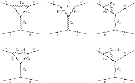
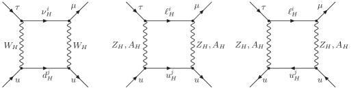
Figure 4: Diagrams contributing to $\tau\to\mu\pi$ in the LHT model. Similar diagrams, but with $d$ quarks in the final state, also contribute.

The diagrams for $\tau\to\mu\pi$ are shown in Fig. 4. As $\pi^{0}$ has the following flavour structure

$$\pi^{0}=\frac{\bar{u}u-\bar{d}d}{\sqrt{2}}\,,$$ (4.3)

there are two sets of diagrams, with $\bar{u}u$ and $\bar{d}d$ in the final state. The corresponding effective Hamiltonians can directly be obtained from [3]. They involve the short-distance functions $\bar{X}_{\text{odd}}^{\tau\mu}$ and $-\bar{Y}_{\text{odd}}^{\tau\mu}$ for $\bar{u}u$ and $\bar{d}d$, respectively. Taking into account the opposite sign that is conventionally chosen to define the two short distance functions, the effective Hamiltonian that includes both sets of diagrams is simply given as follows

$${\cal H}_{\rm eff}=\frac{G_{F}}{\sqrt{2}}\frac{\alpha}{2\pi\sin^{2}\theta_{W}}\left(\bar{X}_{\text{odd}}^{\tau\mu}(\bar{u}u)_{V-A}-\bar{Y}_{\text{odd}}^{\tau\mu}(\bar{d}d)_{V-A}\right)(\bar{\mu}\tau)_{V-A}\,.$$ (4.4)

Here $\bar{X}_{\text{odd}}^{\tau\mu}$ and $\bar{Y}_{\text{odd}}^{\tau\mu}$ have the same structure as the functions calculated in [3] in the context of rare $K$ and $B$ decays. Adapting them to the lepton sector we find:

$$\bar{X}_{\text{odd}}^{\tau\mu} = \left[\chi_{2}^{(\tau\mu)}\big{(}J^{u\bar{u}}(y_{2},z)-J^{u\bar{u}}(y_{1},z)\big{)}+\chi_{3}^{(\tau\mu)}\big{(}J^{u\bar{u}}(y_{3},z)-J^{u\bar{u}}(y_{1},z)\big{)}\right],$$ (4.5)

$$\bar{Y}_{\text{odd}}^{\tau\mu} = \left[\chi_{2}^{(\tau\mu)}\big{(}J^{d\bar{d}}(y_{2},z)-J^{d\bar{d}}(y_{1},z)\big{)}+\chi_{3}^{(\tau\mu)}\big{(}J^{d\bar{d}}(y_{3},z)-J^{d\bar{d}}(y_{1},z)\big{)}\right],$$ (4.6)

where

$$J^{u\bar{u}}\left(y_{i},z\right) = \frac{1}{64}\frac{v^{2}}{f^{2}}\bigg{[}y_{i}S_{\text{odd}}+F^{u\bar{u}}(y_{i},z;W_{H})$$ (4.7)

$$\qquad+4\Big{(}G(y_{i},z;Z_{H})+G_{1}(y^{\prime}_{i},z^{\prime};A_{H})+G_{2}(y_{i},z;\eta)\Big{)}\bigg{]},$$

$$J^{d\bar{d}}\left(y_{i},z\right) = \frac{1}{64}\frac{v^{2}}{f^{2}}\bigg{[}{y_{i}}S_{\text{odd}}+F^{d\bar{d}}(y_{i},z;W_{H})$$ (4.8)

$$\qquad-4\Big{(}G(y_{i},z;Z_{H})+G_{1}(y^{\prime}_{i},z^{\prime};A_{H})-G_{2}(y_{i},z;\eta)\Big{)}\bigg{]},$$

$$S_{\text{odd}} = \frac{1}{\varepsilon}+\log\frac{\mu^{2}}{M_{W_{H}}^{2}}\longrightarrow\log\frac{(4\pi f)^{2}}{M_{W_{H}}^{2}}\,,$$ (4.9)

with the functions $F^{u\bar{u}}$, $F^{d\bar{d}}$, $G$, $G_{1}$ and $G_{2}$ given in Appendix B, the leptonic variables $y_{i}$ and $y_{i}^{\prime}$ defined in (3.13) and the analogous variables for degenerate mirror quarks given by

$$z=\frac{{m^{q}_{H}}^{2}}{M_{W_{H}}^{2}}\,,\qquad z^{\prime}=a\,z\,,\quad\eta=\frac{1}{a}\,.$$ (4.10)

As

$$\langle 0|(\bar{u}u)_{V-A}|\pi^{0}\rangle=-\langle 0|(\bar{d}d)_{V-A}|\pi^{0}\rangle=\frac{F_{\pi}p_{\pi}^{\mu}}{\sqrt{2}}\,,$$ (4.11)

where $F_{\pi}\simeq 131\,{\rm MeV}$ is the pion decay constant, we find

$$Br(\tau\to\mu\pi)=\frac{G_{F}^{2}\alpha^{2}F_{\pi}^{2}m_{\tau}^{3}\tau_{\tau}}{128\pi^{3}\sin^{4}\theta_{W}}\,|\bar{X}_{\text{odd}}^{\tau\mu}+\bar{Y}_{\text{odd}}^{\tau\mu}|^{2}\,,$$ (4.12)

with $\tau_{\tau}$ and $m_{\tau}$ being the lifetime and mass of the decaying $\tau$, and neglecting suppressed pion and muon mass contributions of the order $\mathcal{O}(m_{\pi}^{2}/m_{\tau}^{2})$ and $\mathcal{O}(m_{\mu}^{2}/m_{\tau}^{2})$. The branching ratio for the $\tau\to e\pi$ decay can be obtained very easily from (4.12) by simply replacing $(\tau\mu)$ with $(\tau e)$. The generalization of (4.12) to the decays $\tau\to\mu\eta$ and $\tau\to\mu\eta^{\prime}$ is quite straightforward too, although slightly complicated by mixing in the $\eta-\eta^{\prime}$ system.

The understanding of $\eta-\eta^{\prime}$ mixing has largely improved in the last decade mainly thanks to the formulation of a new mixing scheme [46, 47], where not one but two angles are introduced to relate the physical states ($\eta$, $\eta^{\prime}$) to the octet and singlet states ($\eta_{8}$, $\eta_{0}$), as

$$|\eta\rangle=\cos\theta_{8}|\eta_{8}\rangle-\sin\theta_{0}|\eta_{0}\rangle\,,\qquad|\eta^{\prime}\rangle=\sin\theta_{8}|\eta_{8}\rangle+\cos\theta_{0}|\eta_{0}\rangle\,,$$ (4.13)

with

$$|\eta_{8}\rangle=\frac{1}{\sqrt{6}}(|\bar{u}u\rangle+|\bar{d}d\rangle-2|\bar{s}s\rangle)\,,\qquad|\eta_{0}\rangle=\frac{1}{\sqrt{3}}(|\bar{u}u\rangle+|\bar{d}d\rangle+|\bar{s}s\rangle)\,.$$ (4.14)

In this mixing scheme, four independent decay constants are involved. Each of the two physical mesons ($P=\eta,\eta^{\prime}$), in fact, has both octet ($a=8$) and singlet ($a=0$) components, defined by

$$\langle 0|(\bar{q}{\frac{\lambda^{a}}{2}}q)_{V-A}|P(p)\rangle=\frac{F_{P}^{a}p_{\mu}}{\sqrt{2}}\,,$$ (4.15)

where the $SU(3)$ generators $\lambda^{a}$ satisfy the normalization convention $\text{Tr}[\lambda^{a}\lambda^{b}]=2\delta^{ab}$. They are conveniently parameterized [46] in terms of the two mixing angles ($\theta_{8},\theta_{0}$) and two basic decay constants ($F_{8},F_{0}$), as

$$\begin{pmatrix}F_{\eta}^{8}&F_{\eta}^{0}\\ F_{\eta^{\prime}}^{8}&F_{\eta^{\prime}}^{0}\\ \end{pmatrix}\,=\begin{pmatrix}F_{8}\cos\theta_{8}&-F_{0}\sin\theta_{0}\\ F_{8}\sin\theta_{8}&F_{0}\cos\theta_{0}\\ \end{pmatrix}\,.$$ (4.16)

Working in this mixing scheme and generalizing the expression for the $\tau\to\mu\pi$ branching ratio in (4.12), one obtains

$$Br(\tau\to\mu\eta) = \frac{G_{F}^{2}\alpha^{2}F_{\pi}^{2}m_{\tau}^{3}\tau_{\tau}}{128\pi^{3}\sin^{4}\theta_{W}}\,\left|\frac{\cos\theta_{8}}{\sqrt{3}}\frac{F_{8}}{F_{\pi}}(\bar{X}_{\text{odd}}^{\tau\mu}+\bar{Y}_{\text{odd}}^{\tau\mu})-\sqrt{\frac{2}{3}}\sin\theta_{0}\frac{F_{0}}{F_{\pi}}(\bar{X}_{\text{odd}}^{\tau\mu}-2\,\bar{Y}_{\text{odd}}^{\tau\mu})\right|^{2}\,,$$

$$Br(\tau\to\mu\eta^{\prime}) = \frac{G_{F}^{2}\alpha^{2}F_{\pi}^{2}m_{\tau}^{3}\tau_{\tau}}{128\pi^{3}\sin^{4}\theta_{W}}\,\left|\frac{\sin\theta_{8}}{\sqrt{3}}\frac{F_{8}}{F_{\pi}}(\bar{X}_{\text{odd}}^{\tau\mu}+\bar{Y}_{\text{odd}}^{\tau\mu})+\sqrt{\frac{2}{3}}\cos\theta_{0}\frac{F_{0}}{F_{\pi}}(\bar{X}_{\text{odd}}^{\tau\mu}-2\,\bar{Y}_{\text{odd}}^{\tau\mu})\right|^{2}\,.$$

We conclude this section noting that the function $S_{\text{odd}}$ in (4.9) represents a left-over singularity that signals some sensitivity of the final results to the UV completion of the theory. This issue is known from the study of electroweak precision constraints [11] and has been discussed in detail in the context of the LH model without T-parity [20] and, more recently, also with T-parity [3]. We refer to the latter paper for a detailed discussion. Here we just mention that, in estimating the contribution of these logarithmic singularities as in (4.9), we have assumed the UV completion of the theory not to have a complicated flavour pattern or at least that it has no impact below the cut-off. Clearly, this additional assumption lowers the predictive power of the theory. In spite of that, we believe that the general picture of LFV processes presented here is only insignificantly shadowed by this general property of non-linear sigma models.

5 $\mu^{-}\to e^{-}e^{+}e^{-}$, $\tau^{-}\to\mu^{-}\mu^{+}\mu^{-}$ and $\tau^{-}\to e^{-}e^{+}e^{-}$

Next, we will consider the decay $\mu^{-}\to e^{-}e^{+}e^{-}$, for which the experimental upper bound reads [48]

$$Br(\mu^{-}\to e^{-}e^{+}e^{-})<1.0\cdot 10^{-12}\,.$$ (5.1)

This decay is governed, analogously to the $b\to s\mu^{+}\mu^{-}$ transition, analyzed in the LHT model already in [3], by contributions from $\gamma$- and $Z^{0}$-penguins and by box diagrams. However, the fact that now in the final state two identical particles are present does not allow to use directly the known final expressions for $b\to s\mu^{+}\mu^{-}$, although some intermediate results from the latter decay turned out to be useful here. Also the general result for $\mu^{-}\to e^{-}e^{+}e^{-}$ obtained in [49], which has been corrected in [29, 31], turned out to be very helpful.

Performing the calculation in the unitary gauge, where we found the contribution from the $Z^{0}$-penguin to vanish [3], we find for the relevant amplitudes from photon penguins and box diagrams:

$$\mathcal{A}_{\gamma^{\prime}} = \frac{G_{F}}{\sqrt{2}}\frac{e^{2}}{8\pi^{2}}\frac{1}{q^{2}}\bar{D}^{\prime\,\mu e}_{\text{odd}}\left[\bar{e}(p_{1})(m_{\mu}i\sigma_{\alpha\beta}q^{\beta}(1+\gamma_{5}))\mu(p)\right]\otimes\left[\bar{e}(p_{2})\gamma^{\alpha}e(p_{3})\right]$$ (5.2)

$$\hskip 56.9055pt-(p_{1}\leftrightarrow p_{2})\,,\qquad$$

$$\mathcal{A}_{\gamma} = -\left[4\frac{G_{F}}{\sqrt{2}}\frac{e^{2}}{8\pi^{2}}\bar{Z}^{\mu e}_{\text{odd}}\left[\bar{e}(p_{1})\gamma_{\alpha}(1-\gamma_{5})\mu(p)\right]\otimes\left[\bar{e}(p_{2})\gamma^{\alpha}e(p_{3})\right]-(p_{1}\leftrightarrow p_{2})\right]\,,\qquad$$ (5.3)

$$\mathcal{A}_{\text{box}} = 2\frac{G_{F}}{\sqrt{2}}\frac{\alpha}{2\pi\sin^{2}\theta_{W}}\bar{Y}^{\mu e}_{e,\text{odd}}\left[\bar{e}(p_{1})\gamma_{\alpha}(1-\gamma_{5})\mu(p)\right]\otimes\left[\bar{e}(p_{2})\gamma^{\alpha}(1-\gamma_{5})e(p_{3})\right]\,.$$ (5.4)

The function $\bar{D}^{\prime\,\mu e}_{\text{odd}}$ is given in (3.19), while the functions $\bar{Y}_{e,\text{odd}}^{\mu e}$ and $\bar{Z}_{\text{odd}}^{\mu e}$ can easily be obtained from those calculated in [3]. The analogy with the $b\to s\mu^{+}\mu^{-}$ decay, together with the observation that the $\mu^{-}\to e^{-}e^{+}e^{-}$ decay in question involves only leptons in both the initial and final states, allow us to write

$$\bar{Y}_{e,\text{odd}}^{\mu e} = \chi_{2}^{(\mu e)}\sum_{i=1}^{3}|V_{H\ell}^{ie}|^{2}\left[J^{d\bar{d}}(y_{2},y_{i})-J^{d\bar{d}}(y_{1},y_{i})\right]$$ (5.5)

$$+\,\chi_{3}^{(\mu e)}\sum_{i=1}^{3}|V_{H\ell}^{ie}|^{2}\left[J^{d\bar{d}}(y_{3},y_{i})-J^{d\bar{d}}(y_{1},y_{i})\right]$$

with $J^{d\bar{d}}$ given in (4.8). Following a similar reasoning we can write for the $\bar{Z}_{\text{odd}}^{\mu e}$ function

$$\bar{Z}_{\rm odd}^{\mu e}=\bigg{[}\chi^{(\mu e)}_{2}\big{(}Z_{\rm odd}(y_{2})-Z_{\rm odd}(y_{1})\big{)}+\chi^{(\mu e)}_{3}\big{(}Z_{\rm odd}(y_{3})-Z_{\rm odd}(y_{1})\big{)}\bigg{]}\,,$$ (5.6)

where

$$Z_{\rm odd}(y_{i})=C_{\rm odd}(y_{i})+\frac{1}{4}D_{\rm odd}(y_{i})\,.$$ (5.7)

The explicit expressions of the $C_{\text{odd}}$ and $D_{\text{odd}}$ functions are given in Appendix B. Here, we just note that as a consequence of the charge difference between the leptons involved in $\mu^{-}\to e^{-}e^{+}e^{-}$ and the quarks involved in $b\to s\mu^{+}\mu^{-}$, $D_{\rm odd}$ in (5.7) differs from the analogous function found in [3].

Comparing these expressions to the general expressions for the amplitudes given in [49, 31], we easily obtain $\Gamma(\mu^{-}\to e^{-}e^{+}e^{-})$. Normalizing by $\Gamma(\mu^{-}\to e^{-}\bar{\nu}_{e}\nu_{\mu})$, we find the branching ratio for the decay $\mu^{-}\to e^{-}e^{+}e^{-}$ to be

$$Br(\mu^{-}\to e^{-}e^{+}e^{-}) = \frac{\Gamma(\mu^{-}\to e^{-}e^{+}e^{-})}{\Gamma(\mu^{-}\to e^{-}\bar{\nu}_{e}\nu_{\mu})}$$ (5.8)

$$= \frac{\alpha^{2}}{\pi^{2}}\bigg{[}3\left|\bar{Z}^{\mu e}_{\text{odd}}\right|^{2}+3\,\text{Re}\left(\bar{Z}^{\mu e}_{\text{odd}}(\bar{D}^{\prime\,\mu e}_{\text{odd}})^{*}\right)+\left|\bar{D}^{\prime\,\mu e}_{\text{odd}}\right|^{2}\left(\log\frac{m_{\mu}}{m_{e}}-\frac{11}{8}\right)$$

$$\qquad+\frac{1}{2\sin^{4}\theta_{W}}\left|\bar{Y}^{\mu e}_{e,\text{odd}}\right|^{2}-\frac{2}{\sin^{2}\theta_{W}}\text{Re}\left(\bar{Z}^{\mu e}_{\text{odd}}(\bar{Y}^{\mu e}_{e,\text{odd}})^{*}\right)$$

$$\qquad-\frac{1}{\sin^{2}\theta_{W}}\text{Re}\left(\bar{D}^{\prime\,\mu e}_{\text{odd}}(\bar{Y}^{\mu e}_{e,\text{odd}})^{*}\right)\bigg{]}\,.$$

For $\tau^{-}\to\mu^{-}\mu^{+}\mu^{-}$ we make the following replacements in (5.2)–(5.8):

$$V_{H\ell}^{ie}\to V_{H\ell}^{i\mu}\,,\qquad(\mu e)\to(\tau\mu)\,,\qquad m_{\mu}\to m_{\tau}\,,\qquad m_{e}\to m_{\mu}\,,$$ (5.9)

so that, in particular, $\bar{Y}^{\tau\mu}_{\mu,\text{odd}}$ is now present. Furthermore, in (5.8) the normalization $\Gamma(\mu^{-}\to e^{-}\nu_{\mu}\bar{\nu}_{e})$ is replaced by $\Gamma(\tau^{-}\to\mu^{-}\nu_{\tau}\bar{\nu}_{\mu})$, so that the final result for $Br(\tau^{-}\to\mu^{-}\mu^{+}\mu^{-})$ contains an additional factor $Br(\tau^{-}\to\mu^{-}\nu_{\tau}\bar{\nu}_{\mu})$. In the case of $\tau^{-}\to e^{-}e^{+}e^{-}$ the replacements in (5.5)–(5.8) amount only to

$$(\mu e)\to(\tau e)\,,\qquad m_{\mu}\to m_{\tau}\,,$$ (5.10)

having now $\bar{Y}^{\tau e}_{e,\text{odd}}$, and in (5.8) $\Gamma(\mu^{-}\to e^{-}\nu_{\mu}\bar{\nu}_{e})$ is replaced by $\Gamma(\tau^{-}\to e^{-}\nu_{\tau}\bar{\nu}_{e})$ and an additional factor $Br(\tau^{-}\to e^{-}\nu_{\tau}\bar{\nu}_{e})$ appears. In doing this we neglect in all three expressions $m_{e,\mu}$ with respect to $m_{\tau}$.

6 $\bm{\mu-e}$ Conversion in Nuclei

Similarly to the decays $\mu\to e\gamma$ and $\mu^{-}\to e^{-}e^{+}e^{-}$, stringent experimental upper bounds on $\mu-e$ conversion in nuclei exist. In particular, the experimental upper bound on $\mu-e$ conversion in ${}^{48}_{22}\text{Ti}$ reads [35]

$$R(\mu\text{Ti}\to e\text{Ti})<4.3\cdot 10^{-12}\,,$$ (6.1)

and the dedicated J-PARC experiment PRISM/PRIME should reach a sensitivity of ${\cal O}(10^{-18})$ [34].

A very detailed calculation of the $\mu-e$ conversion rate in various nuclei has been performed in [50], using the methods developed by Czarnecki et al. [51]. It has been emphasized in [50] that the atomic number dependence of the conversion rate can be used to distinguish between different theoretical models of LFV. Useful general formulae can also be found in [49].

We have calculated the $\mu-e$ conversion rate in nuclei in the LHT model using the general model-independent formulae of both [49] and [50]. We have checked numerically that, for relatively light nuclei such as Ti, both results agree within 10%. Therefore, we will give the result for $\mu-e$ conversion in nuclei derived from the general expression given in [49], as it has a more transparent structure than the one of [50].

Following a similar reasoning as in the previous section, we find from (58) of [49]

$$\Gamma(\mu\text{X}\to e\text{X}) = \frac{G_{F}^{2}}{8\pi^{4}}\alpha^{5}\frac{Z_{\text{eff}}^{4}}{Z}|F(q)|^{2}m_{\mu}^{5}$$ (6.2)

$$\cdot\left|Z\left(4\bar{Z}^{\mu e}_{\text{odd}}+\bar{D}^{\prime\,\mu e}_{\text{odd}}\right)-(2Z+N)\frac{\bar{X}^{\mu e}_{\text{odd}}}{\sin^{2}\theta_{W}}+(Z+2N)\frac{\bar{Y}^{\mu e}_{\text{odd}}}{\sin^{2}\theta_{W}}\right|^{2}\,,\qquad$$

where $\bar{X}^{\mu e}_{\text{odd}}$ and $\bar{Y}^{\mu e}_{\text{odd}}$ are obtained from (4.5) and (4.6) by making the replacement $(\tau\mu)\to(\mu e)$, and $\bar{D}^{\prime\,\mu e}_{\text{odd}}$ and $\bar{Z}^{\mu e}_{\text{odd}}$ are given in (3.19) and (5.6), respectively. $Z$ and $N$ denote the proton and neutron number of the nucleus. $Z_{\text{eff}}$ has been determined in [52] and $F(q^{2})$ is the nucleon form factor. For $\text{X}={}^{48}_{22}\text{Ti}$, $Z_{\text{eff}}=17.6$ and $F(q^{2}\simeq-m_{\mu}^{2})\simeq 0.54$ [53].

The $\mu-e$ conversion rate $R(\mu\text{X}\to e\text{X})$ is then given by

$$R(\mu\text{X}\to e\text{X})=\frac{\Gamma(\mu\text{X}\to e\text{X})}{\Gamma^{\text{X}}_{\text{capture}}}\,,$$ (6.3)

with $\Gamma^{\text{X}}_{\text{capture}}$ being the $\mu$ capture rate of the element X. The experimental value is given by $\Gamma^{\text{Ti}}_{\text{capture}}=(2.590\pm 0.012)\cdot 10^{6}\,\text{s}^{-1}$ [54].

In our numerical analysis of Section 12 we will restrict ourselves to $\mu-e$ conversion in ${}^{48}_{22}\text{Ti}$, for which the most stringent experimental upper bound exists and where the approximations entering (6.2) work very well. For details, we refer the reader to [49, 50, 53].

7 $\bm{K_{L,S}\to\mu e}$ and $\bm{K_{L,S}\to\pi^{0}\mu e}$ in the LHT Model

The rare decay $K_{L}\to\mu e$ is well known from the studies of the Pati-Salam (PS) model [55], where it proceeds through a tree level leptoquark exchange in the t-channel. The stringent upper bound on its rate [56]

$$Br(K_{L}\to\mu e)=Br(K_{L}\to\mu^{+}e^{-})+Br(K_{L}\to\mu^{-}e^{+})<4.7\cdot 10^{-12}\,,$$ (7.1)

implies the mass of the leptoquark gauge boson to be above $10^{3}\,{\rm TeV}$ [57]. By increasing the weak gauge group of the PS model in the context of the so-called “Petite Unification” [58] and placing ordinary fermions in multiplets with heavy new fermions, and not with the ordinary SM fermions as in the PS model, it is possible to avoid tree level contributions to $K_{L}\to\mu e$ so that the process is dominated by the box diagrams with new heavy gauge bosons, heavy quarks and heavy leptons exchanged. The relevant masses of these particles can then be decreased to ${\cal O}(1\,{\rm TeV})$ without violating the bound in (7.1).

In the SM the decay $K_{L}\to\mu e$ is forbidden at the tree level but can proceed through box diagrams in the case of non-degenerate neutrino masses. Similarly to $\mu\to e\gamma$ it is too small to be measured.

In the LHT model as well, $K_{L}\to\mu e$ appears first at one loop level. It proceeds through the diagrams shown in Fig. 5 that should be compared with very similar diagrams in Fig. 1 of [14] contributing to particle-antiparticle mixing in the T-odd sector of the LHT model. The main difference is the appearance of leptons in the lower part of the box diagrams instead of quarks, leading to a different structure of the loop functions once the unitarity of the matrices $V_{Hd}$ and $V_{H\ell}$ has been used.

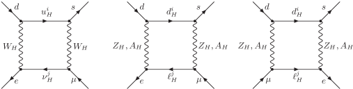
Figure 5: Diagrams contributing to $K_{L}\to\mu^{+}e^{-}$ in the LHT model. Similar diagrams describe $K_{L}\to\mu^{-}e^{+}$.

The effective Hamiltonian for $K_{L}\to\mu e$ can be directly obtained from (3.11) of [14] by removing the QCD factor $\eta_{2}$, appropriately changing the CKM-like factors and the arguments of the short distance functions and multiplying by 2 to correct for a different combinatorial factor.

Taking into account that both the $\mu^{+}e^{-}$ and $\mu^{-}e^{+}$ final states are experimentally detected, the relevant effective Hamiltonian reads

$${\cal H}_{\rm eff} = \frac{G_{F}^{2}}{32\pi^{2}}M_{W_{L}}^{2}\frac{v^{2}}{f^{2}}\sum_{i,j}\xi^{(K)}_{i}F_{H}(z_{i},y_{j})\left[\chi^{(\mu e)}_{j}(\bar{s}d)_{V-A}(\bar{e}\mu)_{V-A}\right.$$ (7.2)

$$\hskip 156.49014pt+\left.{\chi^{(\mu e)}_{j}}^{*}(\bar{s}d)_{V-A}(\bar{\mu}e)_{V-A}\right]+h.c.\,,$$

where $\chi^{(\mu e)}_{i}$ and $y_{i}$ are defined in (2.8) and (3.13), and $\xi_{i}^{(K)}$ and $z_{i}$ belong to the quark sector and are defined as

$$\xi_{i}^{(K)}=V^{*is}_{Hd}V^{id}_{Hd}\,,\qquad z_{i}=\frac{{m^{q}_{Hi}}^{2}}{M_{W_{H}}^{2}}\,.$$ (7.3)

The short distance functions read

$$F_{H}(z_{i},y_{j})=F(z_{i},y_{j};W_{H})+G(z_{i},y_{j};Z_{H})+A_{1}(z_{i},y_{j};Z_{H})+A_{2}(z_{i},y_{j};Z_{H})\,,$$ (7.4)

where the different contributions correspond to “$WW$”, “$ZZ$”, “$AA$” and “$ZA$” diagrams, respectively. Explicit expressions for the functions $F$, $G$, $A_{1}$ and $A_{2}$ can be found in Appendix B.

Using the unitarity of the $V_{Hd}$ and $V_{H\ell}$ matrices we find

$${\cal H}_{\rm eff} = \frac{G_{F}^{2}}{32\pi^{2}}M_{W_{L}}^{2}\frac{v^{2}}{f^{2}}\Bigg{\{}\Big{[}\chi_{2}^{(\mu e)}\xi_{2}^{(K)}R(z_{2},z_{1},y_{1},y_{2})+\chi_{3}^{(\mu e)}\xi_{3}^{(K)}R(z_{3},z_{1},y_{1},y_{3})$$ (7.5)

$$\qquad+\,\chi_{2}^{(\mu e)}\xi_{3}^{(K)}R(z_{3},z_{1},y_{1},y_{2})+\chi_{3}^{(\mu e)}\xi_{2}^{(K)}R(z_{2},z_{1},y_{1},y_{3})\Big{]}(\bar{s}d)_{V-A}(\bar{e}\mu)_{V-A}$$

$$+\,\Big{[}{\chi_{2}^{(\mu e)}}^{*}\xi_{2}^{(K)}R(z_{2},z_{1},y_{1},y_{2})+{\chi_{3}^{(\mu e)}}^{*}\xi_{3}^{(K)}R(z_{3},z_{1},y_{1},y_{3})$$

$$\qquad+\,{\chi_{2}^{(\mu e)}}^{*}\xi_{3}^{(K)}R(z_{3},z_{1},y_{1},y_{2})+{\chi_{3}^{(\mu e)}}^{*}\xi_{2}^{(K)}R(z_{2},z_{1},y_{1},y_{3})\Big{]}(\bar{s}d)_{V-A}(\bar{\mu}e)_{V-A}\Bigg{\}}$$

$$+\,h.c.\,,\qquad$$

where

$$R(z_{i},z_{j},y_{k},y_{l}) = F_{H}(z_{i},y_{l})+F_{H}(z_{j},y_{k})-F_{H}(z_{j},y_{l})-F_{H}(z_{i},y_{k})\,.$$ (7.6)

We remark that the relevant operators differ from $(\bar{d}\gamma_{\mu}e)(\bar{\mu}\gamma^{\mu}s)$ present in the PS model which is characteristic for transitions mediated by leptoquark exchanges. Therefore, the branching ratio for $K_{L}\to\mu e$ in the LHT model is most straightforwardly obtained from the one for $K_{L}\to\mu^{+}\mu^{-}$ in the SM, after the difference between $\mu^{+}\mu^{-}$ and $\mu e$ has been taken into account.

With the help of (XI.44) and (XXV.1) of [59] we easily find

$$Br(K_{L}\to\mu e) = Br(K_{L}\to\mu^{+}e^{-})+Br(K_{L}\to\mu^{-}e^{+})$$ (7.8)

$$= \frac{G_{F}^{2}}{128\pi^{4}}M_{W_{L}}^{4}\frac{v^{4}}{f^{4}}Br(K^{+}\to\mu^{+}\nu)\frac{\tau(K_{L})}{\tau(K^{+})}\frac{1}{|V_{us}|^{2}}$$

$$\hskip 42.67912pt\cdot\left|\sum_{i,j=2,3}\text{Re}(\xi^{(K)}_{i})\chi^{(\mu e)}_{j}R(z_{i},z_{1},y_{1},y_{j})\right|^{2}\,.$$

Here [43, 60]

$$Br(K^{+}\to\mu^{+}\nu)=(63.44\pm 0.14)\%\,,\quad\frac{\tau(K_{L})}{\tau(K^{+})}=4.117\pm 0.019\,,\quad|V_{us}|=0.225\pm 0.001\,.$$ (7.9)

The corresponding expression for $Br(K_{S}\to\mu e)$ is obtained from (7.8) through the replacements [43]

$$\frac{\tau(K_{L})}{\tau(K^{+})}\longrightarrow\frac{\tau(K_{S})}{\tau(K^{+})}=(7.229\pm 0.014)\cdot 10^{-3}\,,\qquad\text{Re}(\xi_{i}^{(K)})\longrightarrow\text{Im}(\xi_{i}^{(K)})\,.$$ (7.10)

Due to $\tau(K_{S})\ll\tau(K_{L})$, the branching ratio $Br(K_{S}\to\mu e)$ is expected to be typically by two orders of magnitude smaller than $Br(K_{L}\to\mu e)$ unless $\text{Im}(\xi_{i}^{(K)})\gg\text{Re}(\xi_{i}^{(K)})$.

The decay $K_{L}\to\pi^{0}\mu e$ in the LHT model is again governed by the effective Hamiltonian in (7.5). This time it is useful to perform the calculation of the branching ratio in analogy with $K_{L}\rightarrow\pi^{0}\nu\bar{\nu}$ [61]. Removing the overall factor 3 in $Br(K_{L}\rightarrow\pi^{0}\nu\bar{\nu})$ corresponding to three neutrino flavours, we find

$$Br(K_{L}\to\pi^{0}\mu e) = Br(K_{L}\to\pi^{0}\mu^{+}e^{-})+Br(K_{L}\to\pi^{0}\mu^{-}e^{+})$$ (7.11)

$$= \frac{G_{F}^{2}M_{W_{L}}^{4}}{128\pi^{4}}\frac{v^{4}}{f^{4}}Br(K^{+}\to\pi^{0}\mu^{+}\nu)\frac{\tau(K_{L})}{\tau(K^{+})}\frac{1}{|V_{us}|^{2}}$$

$$\hskip 42.67912pt\cdot\left|\sum_{i,j=2,3}\text{Im}(\xi_{i}^{(K)})\chi_{j}^{(\mu e)}R(z_{i},z_{1},y_{1},y_{j})\right|^{2}\,.$$

Here [43],

$$Br(K^{+}\to\pi^{0}\mu^{+}\nu)=(3.32\pm 0.06)\%\,.$$ (7.12)

We note that this time $\text{Im}(\xi_{i}^{(K)})$ instead of $\text{Re}(\xi_{i}^{(K)})$ enters, coming from the difference in sign between the relations

$$\langle\pi^{0}|(\bar{d}s)_{V-A}|\bar{K}^{0}\rangle=-\langle\pi^{0}|(\bar{s}d)_{V-A}|K^{0}\rangle$$ (7.13)

and

$$\langle 0|(\bar{d}s)_{V-A}|\bar{K}^{0}\rangle=+\langle 0|(\bar{s}d)_{V-A}|K^{0}\rangle\,.$$ (7.14)

The corresponding expression for $Br(K_{S}\to\pi^{0}\mu e)$ is obtained from (7.11) through the replacements

$$\frac{\tau(K_{L})}{\tau(K^{+})}\longrightarrow\frac{\tau(K_{S})}{\tau(K^{+})}\,,\qquad\text{Im}(\xi_{i}^{(K)})\longrightarrow\text{Re}(\xi_{i}^{(K)})\,.$$ (7.15)

We would like to emphasize that in deriving the formulae for $Br(K_{L,S}\to\mu e)$ and $Br(K_{L,S}\to\pi^{0}\mu e)$ we have neglected the contributions from CP violation in $K^{0}-\bar{K}^{0}$ mixing (indirect CP violation). For instance in the case of $Br(K_{L}\to\pi^{0}\mu e)$ only CP violation in the amplitude (direct CP violation) has been taken into account. The indirect CP violation alone gives the contribution

$$Br(K_{L}\to\pi^{0}\mu e)^{\text{ind.}}=Br(K_{S}\to\pi^{0}\mu e)|\varepsilon_{K}|^{2}$$ (7.16)

and needs only to be taken into account, together with the interference with the contribution from direct CP violation, for $\text{Im}(\xi_{i}^{(K)})\ll\text{Re}(\xi_{i}^{(K)})$. The latter case, however, is uninteresting since it corresponds to an unmeasurably small branching ratio. This should be contrasted with the case of $K_{L}\to\pi^{0}e^{+}e^{-}$, where the indirect CP violation turns out to be dominant [62]. The origin of the difference is that photon penguins, absent in $K_{L}\to\pi^{0}\mu e$, are present in $K_{L}\to\pi^{0}e^{+}e^{-}$ and the structure of ${\cal H}_{\rm eff}$ is rather different from (7.5). Moreover, while the estimate of indirect CP violation to $K_{L}\to\pi^{0}\mu e$ in the LHT model can be done perturbatively, this is not the case for $K_{L}\to\pi^{0}e^{+}e^{-}$, where the matrix elements of the usual $\Delta F=1$ four quark operators have to be taken into account together with renormalization group effects at scales below $M_{W}$.

In summary the branching ratios for $Br(K_{L,S}\to\mu e)$ and $Br(K_{L,S}\to\pi^{0}\mu e)$ in the LHT model can be calculated fully in perturbation theory and are thus as theoretically clean as $K_{L}\rightarrow\pi^{0}\nu\bar{\nu}$. As seen in the formulae (7.8), (7.10), (7.11) and (7.15) above, $Br(K_{L}\to\mu e)$ and $Br(K_{S}\to\pi^{0}\mu e)$ are governed by $\text{Re}(\xi_{i}^{(K)})$, while $Br(K_{S}\to\mu e)$ and $Br(K_{L}\to\pi^{0}\mu e)$ by $\text{Im}(\xi_{i}^{(K)})$. Neglecting the indirect CP violation, we find then that in the so-called “$K$-scenario” of [3], the T-odd contributions to $Br(K_{L}\to\mu e)$ and $Br(K_{S}\to\pi^{0}\mu e)$ are highly suppressed, while $Br(K_{S}\to\mu e)$ and $Br(K_{L}\to\pi^{0}\mu e)$ are generally non-vanishing. The opposite is true in the case of the “$B_{s}$-scenario” in which only $Br(K_{L}\to\mu e)$ and $Br(K_{S}\to\pi^{0}\mu e)$ differ significantly from zero.

This discussion shows that the measurements of $Br(K_{L}\to\mu e)$ and $Br(K_{L}\to\pi^{0}\mu e)$ will transparently shed some light on the complex phases present in the mirror quark sector, and from the point of view of the LHT model, the measurement of $Br(K_{L}\to\pi^{0}\mu e)$ at the level of $10^{-15}$ will be a clear signal of new CP-violating phases at work.

8 $B_{d,s}\rightarrow\mu e$, $B_{d,s}\rightarrow\tau e$ and $B_{d,s}\rightarrow\tau\mu$

The decays of neutral $B$-mesons to two different charged leptons proceed similarly to the $K_{L}\rightarrow\mu e$ decay discussed in Section 7. The effective Hamiltonian describing these processes receive again contributions only from box diagrams. For the $B_{d}\rightarrow\mu e$ decay, it reads

$${\cal H}_{\rm eff}(B_{d}\rightarrow\mu e) = \frac{G_{F}^{2}}{32\pi^{2}}M_{W_{L}}^{2}\frac{v^{2}}{f^{2}}\sum_{i,j}\xi_{i}^{(d)}F_{H}(z_{i},y_{j})\left[\chi^{(\mu e)}_{j}(\bar{b}d)_{V-A}(\bar{e}\mu)_{V-A}\right.$$ (8.1)

$$\hskip 42.67912pt\left.+\chi^{(\mu e)*}_{j}(\bar{b}d)_{V-A}(\bar{\mu}e)_{V-A}\right]\,,$$

with $\xi_{i}^{(d)}=V_{Hd}^{ib*}V_{Hd}^{id}$. Using the unitarity of the $V_{Hd}$ and $V_{H\ell}$ matrices, it becomes

$${\cal H}_{\rm eff}(B_{d}\rightarrow\mu e) = \frac{G_{F}^{2}}{32\pi^{2}}M_{W_{L}}^{2}\frac{v^{2}}{f^{2}}\sum_{i,j=2,3}\xi_{i}^{(d)}R(z_{i},z_{1},y_{1},y_{j})\left[\chi_{j}^{(\mu e)}(\bar{b}d)_{V-A}(\bar{e}\mu)_{V-A}\right.$$ (8.2)

$$\hskip 42.67912pt\left.+\chi_{j}^{(\mu e)*}(\bar{b}d)_{V-A}(\bar{\mu}e)_{V-A}\right]\,,\qquad$$

with $R(z_{i},z_{j},y_{k},y_{l})$ being the combination of short distance functions defined in (7.6).

The effective Hamiltonians describing the remaining decays have a similar structure and can easily be derived from ${\cal H}_{\rm eff}(B_{d}\rightarrow\mu e)$ in (8.2) through the following replacements

$${\cal H}_{\rm eff}(B_{s}\rightarrow\mu e) : \qquad\xi_{i}^{(d)}\rightarrow\xi_{i}^{(s)}\,,$$

$${\cal H}_{\rm eff}(B_{d}\rightarrow\tau e) : \qquad\chi_{j}^{(\mu e)}\rightarrow\chi_{j}^{(\tau e)}\,,$$

$${\cal H}_{\rm eff}(B_{s}\rightarrow\tau e) : \qquad\xi_{i}^{(d)}\rightarrow\xi_{i}^{(s)}\,,\chi_{j}^{(\mu e)}\rightarrow\chi_{j}^{(\tau e)}\,,$$

$${\cal H}_{\rm eff}(B_{d}\rightarrow\tau\mu) : \qquad\chi_{j}^{(\mu e)}\rightarrow\chi_{j}^{(\tau\mu)}\,,$$

$${\cal H}_{\rm eff}(B_{s}\rightarrow\tau\mu) : \qquad\xi_{i}^{(d)}\rightarrow\xi_{i}^{(s)}\,,\chi_{j}^{(\mu e)}\rightarrow\chi_{j}^{(\tau\mu)}\,.$$ (8.3)

The effective Hamiltonians for the $\bar{B}_{d,s}$ decays are simply given by the hermitian conjugates of the corresponding expressions in (8.2) and (8.3).

In calculating the corresponding branching ratios, it is important to observe that while in $K_{L}\rightarrow\mu e$ the decaying meson, $K_{L}\simeq(\bar{s}d+\bar{d}s)/\sqrt{2}$, is a mixture of flavour eigenstates, the decaying $B_{d,s}$ mesons are instead flavour eigenstates (e. g. $B_{d}=\bar{b}d$). For this reason, in $Br(K_{L}\rightarrow\mu e)$ the two conjugate contributions of ${\cal H}_{\rm eff}$ combine together, while in $B_{d,s}$ decays only one contribution enters, with the conjugate one describing $\bar{B}_{d,s}$ decays. With this consideration in mind, starting from $Br(K_{L}\rightarrow\mu e)$ in (7.8), one can straightforwardly find the following expressions

$$Br(\bar{B}_{d}\rightarrow\mu e) = Br(B_{d}\rightarrow\mu e)=Br(B_{d}\rightarrow\mu^{+}e^{-})+Br(B_{d}\rightarrow\mu^{-}e^{+})$$

$$= \frac{G_{F}^{2}M_{W_{L}}^{4}}{512\pi^{4}|V_{ub}|^{2}}\frac{v^{4}}{f^{4}}\frac{\tau(B_{d})}{\tau(B^{+})}Br(B^{+}\rightarrow\mu^{+}\nu_{\mu})$$

$$\cdot\left[\left|\sum_{i,j=2,3}\xi_{i}^{(d)}\chi_{j}^{(\mu e)}R(z_{i},z_{1},y_{1},y_{j})\right|^{2}+\left|\sum_{i,j=2,3}\xi_{i}^{(d)}\chi_{j}^{(\mu e)*}R(z_{i},z_{1},y_{1},y_{j})\right|^{2}\right]\,,$$

$$Br(\bar{B}_{s}\rightarrow\mu e) = Br(B_{s}\rightarrow\mu e)=Br(B_{s}\rightarrow\mu^{+}e^{-})+Br(B_{s}\rightarrow\mu^{-}e^{+})$$ (8.5)

$$= \frac{G_{F}^{2}M_{W_{L}}^{4}}{512\pi^{4}|V_{ub}|^{2}}\frac{v^{4}}{f^{4}}\frac{\tau(B_{s})}{\tau(B^{+})}\frac{M_{B_{s}}}{M_{B_{d}}}\frac{F_{B_{s}}^{2}}{F_{B_{d}}^{2}}Br(B^{+}\rightarrow\mu^{+}\nu_{\mu})$$

$$\cdot\left[\left|\sum_{i,j=2,3}\xi_{i}^{(s)}\chi_{j}^{(\mu e)}R(z_{i},z_{1},y_{1},y_{j})\right|^{2}+\left|\sum_{i,j=2,3}\xi_{i}^{(s)}\chi_{j}^{(\mu e)*}R(z_{i},z_{1},y_{1},y_{j})\right|^{2}\right]\,,$$

$$Br(\bar{B}_{d}\rightarrow\tau e) = Br(B_{d}\rightarrow\tau e)=Br(B_{d}\rightarrow\tau^{+}e^{-})+Br(B_{d}\rightarrow\tau^{-}e^{+})$$

$$= \frac{G_{F}^{2}M_{W_{L}}^{4}}{512\pi^{4}|V_{ub}|^{2}}\frac{v^{4}}{f^{4}}\frac{\tau(B_{d})}{\tau(B^{+})}Br(B^{+}\rightarrow\tau^{+}\nu_{\tau})$$

$$\cdot\left[\left|\sum_{i,j=2,3}\xi_{i}^{(d)}\chi_{j}^{(\tau e)}R(z_{i},z_{1},y_{1},y_{j})\right|^{2}+\left|\sum_{i,j=2,3}\xi_{i}^{(d)}\chi_{j}^{(\tau e)*}R(z_{i},z_{1},y_{1},y_{j})\right|^{2}\right]\,,$$

$$Br(\bar{B}_{s}\rightarrow\tau e) = Br(B_{s}\rightarrow\tau e)=Br(B_{s}\rightarrow\tau^{+}e^{-})+Br(B_{s}\rightarrow\tau^{-}e^{+})$$

$$= \frac{G_{F}^{2}M_{W_{L}}^{4}}{512\pi^{4}|V_{ub}|^{2}}\frac{v^{4}}{f^{4}}\frac{\tau(B_{s})}{\tau(B^{+})}\frac{M_{B_{s}}}{M_{B_{d}}}\frac{F_{B_{s}}^{2}}{F_{B_{d}}^{2}}Br(B^{+}\rightarrow\tau^{+}\nu_{\tau})$$

$$\cdot\left[\left|\sum_{i,j=2,3}\xi_{i}^{(s)}\chi_{j}^{(\tau e)}R(z_{i},z_{1},y_{1},y_{j})\right|^{2}+\left|\sum_{i,j=2,3}\xi_{i}^{(s)}\chi_{j}^{(\tau e)*}R(z_{i},z_{1},y_{1},y_{j})\right|^{2}\right]\,,$$

$$Br(\bar{B}_{d}\rightarrow\tau\mu) = Br(B_{d}\rightarrow\tau\mu)=Br(B_{d}\rightarrow\tau^{+}\mu^{-})+Br(B_{d}\rightarrow\tau^{-}\mu^{+})$$

$$= \frac{G_{F}^{2}M_{W_{L}}^{4}}{512\pi^{4}|V_{ub}|^{2}}\frac{v^{4}}{f^{4}}\frac{\tau(B_{d})}{\tau(B^{+})}Br(B^{+}\rightarrow\tau^{+}\nu_{\tau})$$

$$\cdot\left[\left|\sum_{i,j=2,3}\xi_{i}^{(d)}\chi_{j}^{(\tau\mu)}R(z_{i},z_{1},y_{1},y_{j})\right|^{2}+\left|\sum_{i,j=2,3}\xi_{i}^{(d)}\chi_{j}^{(\tau\mu)*}R(z_{i},z_{1},y_{1},y_{j})\right|^{2}\right]\,,$$

$$Br(\bar{B}_{s}\rightarrow\tau\mu) = Br(B_{s}\rightarrow\tau\mu)=Br(B_{s}\rightarrow\tau^{+}\mu^{-})+Br(B_{s}\rightarrow\tau^{-}\mu^{+})$$

$$= \frac{G_{F}^{2}M_{W_{L}}^{4}}{512\pi^{4}|V_{ub}|^{2}}\frac{v^{4}}{f^{4}}\frac{\tau(B_{s})}{\tau(B^{+})}\frac{M_{B_{s}}}{M_{B_{d}}}\frac{F_{B_{s}}^{2}}{F_{B_{d}}^{2}}Br(B^{+}\rightarrow\tau^{+}\nu_{\tau})$$

$$\cdot\left[\left|\sum_{i,j=2,3}\xi_{i}^{(s)}\chi_{j}^{(\tau\mu)}R(z_{i},z_{1},y_{1},y_{j})\right|^{2}+\left|\sum_{i,j=2,3}\xi_{i}^{(s)}\chi_{j}^{(\tau\mu)*}R(z_{i},z_{1},y_{1},y_{j})\right|^{2}\right]\,.$$

Analogously to $Br(K_{L}\rightarrow\mu e)$, we have chosen to normalize the branching ratios in question introducing the branching ratio of a $B^{+}$ leptonic decay. This normalization will become helpful once $Br(B^{+}\rightarrow\mu^{+}\nu_{\mu})$ and $Br(B^{+}\rightarrow\tau^{+}\nu_{\tau})$ are experimentally measured with sufficient accuracy. Currently the measurements for $Br(B^{+}\rightarrow\tau^{+}\nu_{\tau})$ read

$$Br(B^{+}\to\tau^{+}\nu_{\tau})=\left\{\begin{array}[]{l}\left(1.79^{+0.56+0.39}_{-0.49-0.46}\right)\cdot 10^{-4}\qquad\text{\cite[cite]{[\@@bibref{}{btau-BELLE}{}{}]}}\,,\\ \left(0.88^{+0.68+0.11}_{-0.67-0.11}\right)\cdot 10^{-4}\qquad\text{\cite[cite]{[\@@bibref{}{btau-BABAR}{}{}]}}\,,\end{array}\right.$$ (8.10)

while the experimental upper bound on $Br(B^{+}\rightarrow\mu^{+}\nu_{\mu})$ is given by [65]

$$Br(B^{+}\rightarrow\mu^{+}\nu_{\mu})<6.6\cdot 10^{-6}\qquad(90\%\,\text{C.L.})\,.$$ (8.11)

Therefore, in our numerical analysis in Section 12 we will use the central values of the theoretical predictions for these decays, given by

$$Br(B^{+}\rightarrow\mu^{+}\nu_{\mu}) = \frac{G_{F}^{2}}{8\pi}|V_{ub}|^{2}F_{B_{d}}^{2}M_{B_{d}}m_{\mu}^{2}\tau{(B^{+})}=(3.8\pm 1.1)\cdot 10^{-7}\,,$$ (8.12)

$$Br(B^{+}\to\tau^{+}\nu_{\tau}) = \frac{G_{F}^{2}}{8\pi}|V_{ub}|^{2}F_{B_{d}}^{2}M_{B_{d}}m_{\tau}^{2}\tau{(B^{+})}={(1.1\pm 0.3)\cdot 10^{-4}}\,,$$ (8.13)

where the relevant input parameters are collected in Table 1 of Section 12.

9 $\tau^{-}\to e^{-}\mu^{+}e^{-}$ and $\tau^{-}\to\mu^{-}e^{+}\mu^{-}$

These two decays are of $\Delta L=2$ type and are very strongly suppressed in the SM. In the LHT model they proceed through the box diagrams in Fig. 6.

The effective Hamiltonians for these decays can be obtained from $\Delta B=2$ processes, that is from (3.11) of [14]. In the case of $\tau^{-}\to e^{-}\mu^{+}e^{-}$ we find

$${\cal H}_{\rm eff}=\frac{G_{F}^{2}}{16\pi^{2}}M_{W_{L}}^{2}\frac{v^{2}}{f^{2}}\sum_{i,j}\chi_{i}^{(\tau e)}\chi_{j}^{(\mu e)}F_{H}(y_{i},y_{j})(\bar{e}\tau)_{V-A}(\bar{e}\mu)_{V-A}$$ (9.1)

with the function $F_{H}$ given in (7.4). The additional factor 4 relative to (3.11) of [14] results from the different flavour structure of the operator involved and the two identical particles in the final state.

Figure 6: Diagrams contributing to $\tau^{-}\to e^{-}\mu^{+}e^{-}$ in the LHT model.

The corresponding effective Hamiltonian for $\tau^{-}\to\mu^{-}e^{+}\mu^{-}$ is obtained by simply exchanging $e$ and $\mu$, with $\chi_{j}^{(e\mu)}={\chi_{j}^{(\mu e)}}^{*}$.

The relevant branching ratios can be found by comparing these two decays to the tree level decay $\tau^{-}\to\nu_{\tau}e^{-}\bar{\nu}_{e}$, for which the effective Hamiltonian reads

$${\cal H}_{\rm eff}=\frac{G_{F}}{\sqrt{2}}(\bar{\nu}_{\tau}\tau)_{V-A}(\bar{e}\nu_{e})_{V-A}\,,$$ (9.2)

and yields the decay rate

$$\Gamma(\tau^{-}\to\nu_{\tau}e^{-}\bar{\nu}_{e})=\frac{G_{F}^{2}m_{\tau}^{5}}{192\pi^{3}}\,.$$ (9.3)

For $\tau^{-}\to e^{-}\mu^{+}e^{-}$ we find then

$$Br(\tau^{-}\to e^{-}\mu^{+}e^{-})=\frac{m_{\tau}^{5}\tau_{\tau}}{192\pi^{3}}\left(\frac{G_{F}^{2}M_{W_{L}}^{2}}{16\pi^{2}}\right)^{2}\frac{v^{4}}{f^{4}}\left|\sum_{i,j}\chi_{i}^{(\tau e)}\chi_{j}^{(\mu e)}F_{H}(y_{i},y_{j})\right|^{2},$$ (9.4)

where we neglected $m_{\mu,e}$ with respect to $m_{\tau}$. We have included the factor $1/2$ to take into account the presence of two identical fermions in the final state.

The branching ratio for $\tau^{-}\to\mu^{-}e^{+}\mu^{-}$ is obtained from (9.4) by interchanging $\mu\leftrightarrow e$.

10 $\tau^{-}\to\mu^{-}e^{+}e^{-}$ and $\tau^{-}\to e^{-}\mu^{+}\mu^{-}$

These decays have two types of contributions. First of all they proceed as in $\tau^{-}\to\mu^{-}\mu^{+}\mu^{-}$ and $\tau^{-}\to e^{-}e^{+}e^{-}$ through $\Delta L=1$ penguin and box diagrams. As this time there are no identical particles in the final state, the effective Hamiltonians for these contributions can be directly obtained from the decay $B\to X_{s}\ell^{+}\ell^{-}$. Let us derive explicitly the effective Hamiltonian for $\tau^{-}\to\mu^{-}e^{+}e^{-}$. The generalization to $\tau^{-}\to e^{-}\mu^{+}\mu^{-}$ will then be automatic.

As the QCD corrections are not involved now, only three operators originating in magnetic photon penguins, $Z^{0}$-penguins, standard photon penguins and the relevant box diagrams have to be considered. Keeping the notation from $B\to X_{s}\mu^{+}\mu^{-}$ but translating the quark flavours into lepton flavours these operators are

$$\mathcal{Q}_{7}=\frac{e}{8\pi^{2}}m_{\tau}\bar{\mu}\sigma^{\alpha\beta}(1+\gamma_{5})\tau F_{\alpha\beta}\,,$$ (10.1)

that enters, of course with different external states, also the $\mu\to e\gamma$ decay, and

$$\mathcal{Q}_{9}=(\bar{\mu}\tau)_{V-A}(\bar{e}e)_{V}\,,\qquad\mathcal{Q}_{10}=(\bar{\mu}\tau)_{V-A}(\bar{e}e)_{A}\,.$$ (10.2)

The effective Hamiltonian is then given by

$${\cal H}_{\rm eff}(\tau^{-}\to\mu^{-}e^{+}e^{-})=-\frac{G_{F}}{\sqrt{2}}\left[C_{7}^{\tau\mu}\mathcal{Q}_{7}+C_{9}^{\tau\mu}\mathcal{Q}_{9}+C_{10}^{\tau\mu}\mathcal{Q}_{10}\right]\,.$$ (10.3)

The Wilson coefficient for the operator $\mathcal{Q}_{7}$ can easily be found from Section 3 of the present paper and Section 7 of [3]. We find

$$C_{7}^{\tau\mu}=-\frac{1}{2}\bar{D}^{\prime\,\tau\mu}_{\text{odd}}\,,$$ (10.4)

with $\bar{D}^{\prime\,\tau\mu}_{\text{odd}}$ obtained from (3.19) by replacing $(\mu e)$ with $(\tau\mu)$.

The Wilson coefficients of the operators $\mathcal{Q}_{9}$ and $\mathcal{Q}_{10}$ receive not only contributions from $\Delta L=1$ $\gamma$-penguin, $Z^{0}$-penguin and box diagrams, but also from $\Delta L=2$ box diagrams, as in Section 9. For $C_{9}^{\tau\mu}$ and $C_{10}^{\tau\mu}$ we can then write

$$C_{9}^{\tau\mu}=\frac{\alpha}{2\pi}\tilde{C}_{9}^{\tau\mu}\,,\qquad C_{10}^{\tau\mu}=\frac{\alpha}{2\pi}\tilde{C}_{10}^{\tau\mu}\,,$$ (10.5)

$$\tilde{C}_{9}^{\tau\mu}=\frac{\bar{Y}_{e,\text{odd}}^{\tau\mu}}{\sin^{2}\theta_{W}}-4\bar{Z}_{\text{odd}}^{\mu e}-\Delta_{\tau\mu}\,,\qquad\tilde{C}_{10}^{\tau\mu}=-\frac{\bar{Y}_{e,\text{odd}}^{\tau\mu}}{\sin^{2}\theta_{W}}+\Delta_{\tau\mu}\,,$$ (10.6)

with the functions $\bar{Y}_{e,\text{odd}}^{\tau\mu}$ and $\bar{Z}_{\text{odd}}^{\tau\mu}$ obtained from (5.5) and (5.6) by replacing ($\mu e$) by ($\tau\mu$). $\Delta_{\tau\mu}$ represents the additional $\Delta L=2$ contribution which is not present in the case of $b\to s\ell^{+}\ell^{-}$ and will be explained below. As there are no light fermions in the T-odd sector, the mass independent term present in $C_{9}$ in the case of $b\to s\ell^{+}\ell^{-}$ in (X.5) of [59] is absent here. Effectively this corresponds to setting $\eta=1$ in the latter equation and of course removing QCD corrections.

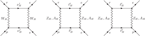
Figure 7: Diagrams of $\Delta L=2$ type contributing to $\tau^{-}\to\mu^{-}e^{+}e^{-}$ in the LHT model.

As already mentioned, also the $\Delta L=2$ diagrams shown in Fig. 7 contribute to this decay. The corresponding effective Hamiltonian can be obtained from (9.1) through the obvious replacements of local operators, removing the symmetry factor 2 and the following change in the mixing factors:

$$\chi_{i}^{(\tau e)}{\chi_{j}^{(\mu e)}}\longrightarrow\chi_{i}^{(\tau e)}{\chi_{j}^{(\mu e)}}^{*}\,,$$ (10.7)

so that we find

$$\Delta_{\tau\mu} = \frac{2\pi}{\alpha}\frac{G_{F}}{32\pi^{2}}\sqrt{2}M_{W_{L}}^{2}\frac{v^{2}}{f^{2}}\sum_{i,j}\chi_{i}^{(\tau e)}{\chi_{j}^{(\mu e)}}^{*}F_{H}(y_{i},y_{j})$$ (10.8)

$$= \frac{1}{16\sin^{2}\theta_{W}}\frac{v^{2}}{f^{2}}\sum_{i,j}\chi_{i}^{(\tau e)}{\chi_{j}^{(\mu e)}}^{*}F_{H}(y_{i},y_{j})\,.$$

Effectively the presence of the diagrams in Fig. 7 introduces corrections to the Wilson coefficients $\tilde{C}_{9}$ and $\tilde{C}_{10}$ in (10.6). As the relevant operator has the structure $(V-A)\otimes(V-A)$, the shifts in $\tilde{C}_{9}$ and $\tilde{C}_{10}$ are equal up to an overall sign.

Finally, introducing

$$\hat{s}=\frac{(p_{e^{+}}+p_{e^{-}})^{2}}{m_{\tau}^{2}}\,,\qquad R^{\tau\mu}(\hat{s})=\frac{\frac{d}{d\hat{s}}{\Gamma(\tau^{-}\to\mu^{-}e^{+}e^{-})}}{\Gamma(\tau^{-}\to\mu^{-}\bar{\nu}_{\mu}\nu_{\tau})}$$ (10.9)

and neglecting $m_{e}$ with respect to $m_{\tau}$ we find for the differential decay rate $R^{\tau\mu}(\hat{s})$

$$R^{\tau\mu}(\hat{s}) = \frac{\alpha^{2}}{4\pi^{2}}(1-\hat{s})^{2}\bigg{[}(1+2\hat{s})\left(|\tilde{C}_{9}^{\tau\mu}|^{2}+|\tilde{C}_{10}^{\tau\mu}|^{2}\right)$$ (10.10)

$$\hskip 71.13188pt+4\left(1+\frac{2}{\hat{s}}\right)|C_{7}^{\tau\mu}|^{2}+12\,\text{Re}\left(C_{7}^{\tau\mu}{(\tilde{C}_{9}^{\tau\mu})}^{*}\right)\bigg{]}\,.$$

The branching ratio is then given as follows:

$$Br(\tau^{-}\to\mu^{-}e^{+}e^{-})=Br(\tau^{-}\to\mu^{-}\bar{\nu}_{\mu}\nu_{\tau})\int_{4m_{e}^{2}/m_{\tau}^{2}}^{1}R^{\tau\mu}(\hat{s})\,d\hat{s}\,.$$ (10.11)

The branching ratio for $\tau^{-}\to e^{-}\mu^{+}\mu^{-}$ can easily be obtained from the above expressions by interchanging $\mu\leftrightarrow e$, where $\chi_{i}^{(e\mu)}={\chi_{i}^{(\mu e)}}^{*}$.

For quasi-degenerate mirror leptons the $\Delta L=1$ part clearly dominates as the GIM-like suppression acts only on one mirror lepton propagator, whereas it acts twice in the $\Delta L=2$ case. Moreover, in the latter case the effective Hamiltonian is quartic in the $V_{H\ell}$ couplings, whereas it is to a very good approximation quadratic in the case of $\Delta L=1$. As these factors are all smaller than 1, quite generally $\Delta L=2$ contributions will then be additionally suppressed by the mixing matrix elements. Consequently, the $\Delta L=1$ part is expected to dominate and the shift $\Delta_{\tau\mu}$ can be neglected. On the other hand, for very special structures of the $V_{H\ell}$ matrix, the double GIM suppression of $\Delta L=2$ with respect to $\Delta L=1$ contributions could be compensated by the $V_{H\ell}$ factors. Therefore it is safer to use the more general expressions given above.

11 $\bm{(g-2)_{\mu}}$ in the LHT Model

The anomalous magnetic moment of the muon $a_{\mu}=(g-2)_{\mu}/2$ provides an excellent test for physics beyond the SM and has been measured very precisely at the E821 experiment [66] in Brookhaven. The latest result of the ${(g-2)}$ Collaboration of E821 reads

$$a_{\mu}^{\rm{exp}}=(11659208.0\pm 6.3)\cdot 10^{-10}\,,$$ (11.1)

whereas the SM prediction is given by [67]

$$a_{\mu}^{\rm{SM}}={a_{\mu}^{\rm{QED}}+a_{\mu}^{\rm{ew}}+a_{\mu}^{\rm{had}}}=(11659180.4\pm 5.1)\cdot 10^{-10}\,.$$ (11.2)

While the QED and electroweak contributions to $a_{\mu}^{\text{SM}}$ are known very precisely [68, 69], the theoretical uncertainty is dominated by the hadronic vacuum polarization and light-by-light contributions. These contributions have been evaluated in [67, 70, 71, 72].

The anomalous magnetic moment $a_{\mu}$ can be extracted from the photon-muon vertex function $\Gamma^{\mu}(p^{\prime},p)$

$$\bar{u}(p^{\prime})\Gamma^{\mu}(p^{\prime},p)u(p)=\bar{u}(p^{\prime})\left[\gamma^{\mu}F_{V}(q^{2})+(p+p^{\prime})^{\mu}F_{M}(q^{2})\right]u(p)\,,$$ (11.3)

where the anomalous magnetic moment of the muon $a_{\mu}$ can be read off as

$$a_{\mu}=-2mF_{M}(0)\,.$$ (11.4)

The diagrams which yield new contributions to $a_{\mu}$ in the LHT model are shown in Fig. 8. They either have a heavy neutral gauge boson ($Z_{H}$ or $A_{H}$) and two heavy charged leptons $\ell_{H}^{i}\,\,(i=1,2,3)$ or two heavy charged gauge bosons ($W_{H}^{\pm}$) and one heavy neutrino $\nu_{H}^{i}\,\,(i=1,2,3)$ running in the loop.

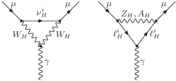
Figure 8: Diagrams contributing to $(g-2)_{\mu}$ in the LHT model.

Calculating the diagrams in Fig. 8 and using the Feynman rules given in [3], the contributions of the new particles for each generation $i=1,2,3$ are found to be:

$$\left[a_{\mu}\right]^{i}_{X=A_{H},Z_{H}} = \frac{1}{2\pi^{2}}\frac{m^{2}_{\mu}}{M^{2}_{X}}\left|C^{i}_{X}\right|^{2}r_{i}\left\{\left(\frac{5}{6}-\frac{5}{2}r_{i}+r_{i}^{2}+\left(r_{i}^{3}-3r_{i}^{2}+2r_{i}\right)\ln\frac{r_{i}-1}{r_{i}}\right)\right.$$ (11.5)

$$\hskip 28.45274pt+\,\frac{{m_{Hi}^{\ell}}^{2}}{2M_{X}^{2}}\left(\frac{5}{6}+\frac{3}{2}r_{i}+r_{i}^{2}+\left(r_{i}^{2}+r_{i}^{3}\right)\ln\frac{r_{i}-1}{r_{i}}\right)\bigg{\}}\,,$$

$$\left[a_{\mu}\right]^{i}_{X=W_{H}} = -\frac{1}{4\pi^{2}}\frac{m^{2}_{\mu}}{M^{2}_{X}}\left|C^{i}_{X}\right|^{2}r_{i}\left\{-2\left(\frac{5}{6}-\frac{3}{2}b_{i}+b_{i}^{2}+\left(b_{i}^{2}-b_{i}^{3}\right)\ln\frac{b_{i}+1}{b_{i}}\right)\right.$$ (11.6)

$$\hskip 28.45274pt-\,\frac{{m_{Hi}^{\ell}}^{2}}{M_{X}^{2}}\left(\frac{5}{6}+\frac{5}{2}b_{i}+b_{i}^{2}-\left(2b_{i}+3b_{i}^{2}+b_{i}^{3}\right)\ln\frac{b_{i}+1}{b_{i}}\right)\Bigg{\}}\,,\qquad$$

where

$$r_{i}=\left(1-\frac{{m_{Hi}^{\ell}}^{2}}{M_{X}^{2}}\right)^{-1},\qquad b=\frac{{m_{Hi}^{\ell}}^{2}}{M_{X}^{2}}\,r_{i}$$ (11.7)

and

$$C^{i}_{A_{H}}=\frac{g^{\prime}}{20}\,V_{H\ell}^{i\mu}\,,\qquad C^{i}_{Z_{H}}=\frac{g}{4}\,V_{H\ell}^{i\mu}\,,\qquad C^{i}_{W_{H}}=\frac{g}{2\sqrt{2}}\,V_{H\ell}^{i\mu}\,.$$ (11.8)

The parameter $m_{Hi}^{\ell}$ in (11.5) and (11.6) denotes the mass of the mirror leptons while $M_{X}$ is the mass of the heavy gauge bosons. We expanded our results in the small parameter $m_{\mu}/M_{X}$. Our results in (11.5) and (11.6) for the muon anomalous magnetic moment are confirmed by the formulae in [73] for general couplings.

Replacing the parameters $r$ and $b$ by the more convenient parameter $y_{i}$, defined in (3.13), leads us to the following expressions

$$\left[a_{\mu}\right]_{Z_{H}} = \frac{\sqrt{2}G_{F}}{32\pi^{2}}\frac{v^{2}}{f^{2}}m_{\mu}^{2}\sum_{i=1}^{3}{\left|V_{H\ell}^{i\mu}\right|^{2}}L_{1}(y_{i})\,,$$ (11.9)

$$\left[a_{\mu}\right]_{A_{H}} = \frac{\sqrt{2}G_{F}}{160\pi^{2}}\frac{v^{2}}{f^{2}}m_{\mu}^{2}\sum_{i=1}^{3}{\left|V_{H\ell}^{i\mu}\right|^{2}}L_{1}(y^{\prime}_{i})\,,$$ (11.10)

$$\left[a_{\mu}\right]_{W_{H}} = \frac{-\sqrt{2}G_{F}}{32\pi^{2}}\frac{v^{2}}{f^{2}}m_{\mu}^{2}\sum_{i=1}^{3}{\left|V_{H\ell}^{i\mu}\right|^{2}}L_{2}(y_{i})\,,$$ (11.11)

where the functions $L_{1}$ and $L_{2}$ are given in Appendix B.

Our final result for ${a_{\mu}}$ in the LHT model therefore is

$$a_{\mu}=\left[a_{\mu}\right]_{\text{SM}}+\frac{\sqrt{2}G_{F}}{32\pi^{2}}\frac{v^{2}}{f^{2}}m_{\mu}^{2}\sum_{i=1}^{3}{\left|V_{H\ell}^{i\mu}\right|^{2}}\left[L_{1}(y_{i})-L_{2}(y_{i})+\frac{1}{5}L_{1}(y_{i}^{\prime})\right]\,.$$ (11.12)

While we disagree with [26], we confirm the result of [27] except that according to us the factors $(V_{H\nu})_{2i}^{*}(V_{H\nu})_{2i}$ and $(V_{H\ell})_{2i}^{*}(V_{H\ell})_{2i}$ in equations (3.22)–(3.24) of that paper should be replaced by $|V_{H\ell}^{i\mu}|^{2}$.

12 Numerical Analysis

12.1 Preliminaries

In contrast to rare meson decays, the number of flavour violating decays in the lepton sector, for which useful constraints exist, is rather limited. Basically only the constraints on $Br(\mu\to e\gamma)$, $Br(\mu^{-}\to e^{-}e^{+}e^{-})$, $R(\mu\text{Ti}\to e\text{Ti})$ and $Br(K_{L}\to\mu e)$ can be mentioned here. The situation may change significantly in the coming years and the next decade through the experiments briefly discussed in the introduction.

$m_{e}=0.5110\,{\rm MeV}$	$\tau(B_{d})/\tau(B^{+})=0.934(7)$
$m_{\mu}=105.66\,{\rm MeV}$	$\tau(B_{s})=1.466(59)\,\text{ps}$
$m_{\tau}=1.7770(3)\,{\rm GeV}$	$\tau(B^{+})=1.638(11)\,\text{ps}$
$\tau_{\tau}=290.6(10)\cdot 10^{-3}\,\text{ps}$	$M_{B_{d}}=5.2794(5)\,{\rm GeV}$
$M_{W}=80.425(38)\,{\rm GeV}$	$M_{B_{s}}=5.3675(18)\,{\rm GeV}$  [43]
$\alpha=1/137$	$|V_{ub}|=3.68(14)\cdot 10^{-3}$ [75]
$G_{F}=1.16637(1)\cdot 10^{-5}\,{\rm GeV}^{-2}$	$F_{8}/F_{\pi}=1.28$ (ChPT)
$\sin^{2}\theta_{W}=0.23122(15)$   [43]	$F_{0}/F_{\pi}=1.18(4)$
$F_{B_{d}}=189(27)\,{\rm MeV}$	$\theta_{8}=-22.2(18)^{\circ}$
$F_{B_{s}}=230(30)\,{\rm MeV}$ [74]	$\theta_{0}=-8.7(21)^{\circ}$ [76]

Table 1: Values of the experimental and theoretical quantities used as input parameters.

In this section we want to analyze numerically various branching ratios that we have calculated in Sections 3–11. In Section 13 we will extend our numerical analysis by studying various ratios of branching ratios and comparing them with those found in the MSSM. Our purpose is not to present a very detailed numerical analysis of all decays, but rather to concentrate on the most interesting ones from the present perspective and indicate rough upper bounds on all calculated branching ratios within the LHT model. To this end we will first set $f=1\,{\rm TeV}$ and consider three benchmark scenarios for the remaining LHT parameters in (2.12), as discussed below.

In Table 1 we collect the values of the input parameters that enter our numerical analysis. In order to simplify the analysis, we will set all input parameters to their central values. As all parameters, except for the decay constants $F_{B_{d,s}}$ and the $\eta-\eta^{\prime}$ mixing angles, are known with quite high precision, including the error ranges in the analysis would amount only to percent effects in the observables considered, which is clearly beyond the scope of our analysis.

12.2 Benchmark Scenarios

We will consider the following three scenarios:

Scenario A (red):

In this scenario we will choose

$$V_{H\ell}=V_{\text{PMNS}}^{\dagger}\,,$$ (12.1)

so that $V_{H\nu}\equiv\mathbbm{1}$, and mirror leptons have no impact on flavour violating observables in the neutrino sector, such as neutrino oscillations. In particular we set the PMNS parameters to [42]

$$\sin\theta_{12}=\sqrt{0.300}\,,\qquad\sin\theta_{13}=\sqrt{0.030}\,,\qquad\sin\theta_{23}=\frac{1}{\sqrt{2}}\,,\qquad\delta_{13}=65^{\circ}\,,$$ (12.2)

which is consistent with the experimental constraints on the PMNS matrix [43]. As no constraints on the PMNS phases exist, we have taken $\delta_{13}$ to be equal to the CKM phase and set the two Majorana phases to zero.

Furthermore, we take the mirror lepton masses to lie in the range

$$300\,{\rm GeV}\leq m^{\ell}_{Hi}\leq 1.5\,{\rm TeV}\,,\qquad{(i=1,2,3)}\,.$$ (12.3)

Scenario B (green):

Here, we take

$$V_{H\ell}=V_{\text{CKM}}\,,$$ (12.4)

so that [75]

$$\theta^{\ell}_{12}=13^{\circ}\,,\qquad\theta^{\ell}_{13}=0.25^{\circ}\,,\qquad\theta^{\ell}_{23}=2.4^{\circ}\,,$$ (12.5)

$$\delta^{\ell}_{12}=0\,,\qquad\delta^{\ell}_{13}=65^{\circ}\,,\qquad\delta^{\ell}_{13}=0\,,$$ (12.6)

and the mirror lepton masses in the range (12.3).

Scenario C (blue):

Here we perform a general scan over the whole parameter space, with the only restriction being the range (12.3) for mirror lepton masses.

At a certain stage we will investigate the dependence on mass splittings in the mirror lepton spectrum.

In the case of $K_{L}\to\mu e$, $B_{d,s}\to\mu e$ and similar decays of Sections 7 and 8, the parameters of the mirror quark sector enter and the constraints from $K$ and $B$ physics, analyzed in [14, 3], have to be taken into account.

12.3 $\mu\to e\gamma$, $\mu^{-}\to e^{-}e^{+}e^{-}$ and $\mu-e$ Conversion

In Fig. 9 we show the correlation between $\mu\to e\gamma$ and $\mu^{-}\to e^{-}e^{+}e^{-}$ in the scenarios in question together with the experimental bounds on these decays. We observe:

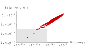
Scenario A

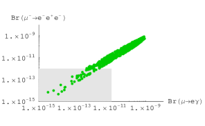
Scenario B

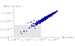
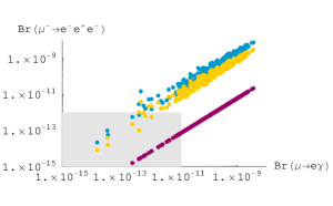
Scenario C

Figure 9: Correlation between $\mu\to e\gamma$ and $\mu^{-}\to e^{-}e^{+}e^{-}$ in the scenarios of Section 12.2. In the right plot of Scenario C we show the contributions to $\mu^{-}\to e^{-}e^{+}e^{-}$ from $\bar{D}_{\text{odd}}^{\prime\,\mu e}$ (purple, lowermost), $\bar{Z}_{\text{odd}}^{\mu e}$ (orange, middle) and $\bar{Y}_{e,\text{odd}}^{\mu e}$ (light-blue, uppermost) separately. The shaded area represents the experimental constraints.

• In Scenario A the great majority of points is outside the allowed range, implying that the $V_{H\ell}$ matrix must be much more hierarchical than $V_{\text{PMNS}}$ in order to satisfy the present upper bounds on $\mu\to e\gamma$ and $\mu^{-}\to e^{-}e^{+}e^{-}$.

• Also in Scenario B most of the points violate the current experimental bounds, although $V_{\text{CKM}}$ is much more hierarchical than $V_{\text{PMNS}}$. The reason is that the CKM hierarchy $s_{13}\ll s_{23}\ll s_{12}$ implies very small effects in transitions between the third and the first generation, like $\tau\to e\gamma$, while allowing relatively large effects in the $\mu\to e$ transitions. Thus in order to satisfy the experimental constraints on $\mu\to e\gamma$ and $\mu^{-}\to e^{-}e^{+}e^{-}$ a very different hierarchy of the $V_{H\ell}$ matrix is required, unless the mirror lepton masses are quasi-degenerate.

• In Scenario C there are more possibilities, but also here a strong correlation between $\mu\to e\gamma$ and $\mu^{-}\to e^{-}e^{+}e^{-}$ is observed. This is easy to understand, as both decays probe dominantly the combinations of $V_{H\ell}$ elements $\chi_{i}^{(\mu e)}$.

• For Scenario C, we also show the contributions to $\mu^{-}\to e^{-}e^{+}e^{-}$ from $\bar{D}_{\text{odd}}^{\prime\,\mu e}$, $\bar{Z}_{\text{odd}}^{\mu e}$ and $\bar{Y}_{e,\text{odd}}^{\mu e}$ separately. We observe that the dominant contributions come from the functions $\bar{Z}_{\text{odd}}^{\mu e}$ and above all $\bar{Y}_{e,\text{odd}}^{\mu e}$, while the contribution of the operator $\mathcal{Q}_{7}$, given by $\bar{D}_{\text{odd}}^{\prime\,\mu e}$, is by roughly two orders of magnitude smaller and thus fully negligible. This should be contrasted with the case of the MSSM where the dipole operator is dominant. We will return to the consequences of this finding in the next section.

• We emphasize that the strong correlation between $\mu\to e\gamma$ and $\mu^{-}\to e^{-}e^{+}e^{-}$ in the LHT model is not a common feature of all extensions of the SM, in which the structure of $\mu^{-}\to e^{-}e^{+}e^{-}$ is generally much more complicated than in the LHT model. It is clear from Fig. 9 that an improved upper bound on $\mu\to e\gamma$ by MEG in 2007 and in particular its discovery will provide important information on $\mu^{-}\to e^{-}e^{+}e^{-}$ within the model in question.

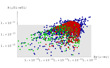
Figure 10: $\mu-e$ conversion rate in ${}^{48}_{22}\text{Ti}$ as a function of $Br(\mu\to e\gamma)$, after imposing the existing constraints on $\mu\to e\gamma$ and $\mu^{-}\to e^{-}e^{+}e^{-}$. The shaded area represents the current experimental upper bound on $R(\mu\text{Ti}\to e\text{Ti})$.

Next, in Fig. 10 we show the correlation between the $\mu-e$ conversion rate in ${}^{48}_{22}\text{Ti}$ and $Br(\mu\to e\gamma)$, after imposing the existing constraints on $\mu\to e\gamma$ and $\mu^{-}\to e^{-}e^{+}e^{-}$. We observe that this correlation is much weaker than the one between $\mu\to e\gamma$ and $\mu^{-}\to e^{-}e^{+}e^{-}$. Furthermore, we find that the $\mu-e$ conversion rate in Ti is likely to be found close to the current experimental upper bound, and that in some regions of the parameter space the latter bound is even the most constraining one.

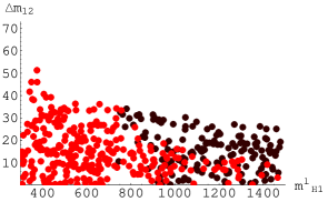
Scenario A

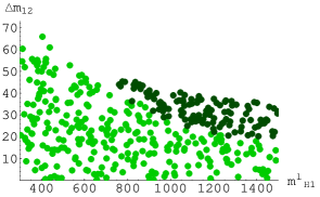
Scenario B

Figure 11: Mirror lepton mass splitting $\Delta m_{12}=|m^{\ell}_{H2}-m^{\ell}_{H1}|$ as a function of $m^{\ell}_{H1}$, after imposing the existing constraints on $\mu\to e\gamma$ and $\mu^{-}\to e^{-}e^{+}e^{-}$. The dark points violate the constraint on $\mu-e$ conversion in Ti, while the light points fulfil also this constraint.

We also show in Fig. 11 the mass splitting $\Delta m_{12}=|m^{\ell}_{H2}-m^{\ell}_{H1}|$ as a function of $m^{\ell}_{H1}$, after imposing the existing constraints on $\mu\to e\gamma$ and $\mu^{-}\to e^{-}e^{+}e^{-}$. We observe that for the scenarios A and B considered here, the first two generations of mirror leptons have to be quasi-degenerate in order to satisfy the experimental constraints. While in the case of Scenario A, $\Delta m_{12}\mathrel{\hbox to0.0pt{\raise 2.20013pt\hbox{$<$}\hss}{\lower 2.20013pt\hbox{$\sim$}}}40\,{\rm GeV}$ is required, $\Delta m_{12}\mathrel{\hbox to0.0pt{\raise 2.20013pt\hbox{$<$}\hss}{\lower 2.20013pt\hbox{$\sim$}}}60\,{\rm GeV}$ is sufficient to fulfil the constraints in Scenario B, provided the mirror lepton masses are relatively small. Generally we find that the allowed mass splittings are larger for smaller values of the mirror lepton masses. This is due to the fact that the functions $J^{u\bar{u}}$ and $J^{d\bar{d}}$, as defined in (4.7) and (4.8), are monotonously increasing, making thus a stronger GIM suppression necessary in the case of large masses. Finally we have studied the impact of the experimental bound on $R(\mu\text{Ti}\to e\text{Ti})$ on the allowed mass splittings. We observe that in particular for large values of the mirror lepton masses, $\mu-e$ conversion turns out to be even more constraining than $\mu\to e\gamma$ and $\mu^{-}\to e^{-}e^{+}e^{-}$.

12.4 $\tau\to\mu\gamma$ and $\tau\to e\gamma$

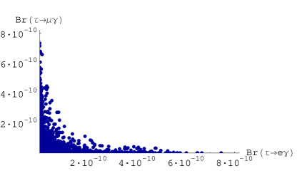
Figure 12: Correlation between $Br(\tau\to e\gamma)$ and $Br(\tau\to\mu\gamma)$.

In Fig. 12 we show the correlation between $Br(\tau\to\mu\gamma)$ and $Br(\tau\to e\gamma)$ in the scenarios considered, imposing the experimental bounds on $\mu\to e\gamma$ and $\mu^{-}\to e^{-}e^{+}e^{-}$. We observe that they both can be individually as high as $\sim 8\cdot 10^{-10}$, but the highest values of $Br(\tau\to\mu\gamma)$ correspond generally to much lower values of $Br(\tau\to e\gamma)$ and vice versa. Still simultaneous values of both branching ratios as high as $2\cdot 10^{-10}$ are possible.

12.5 $\tau\to\mu\pi,\mu\eta,\mu\eta^{\prime}$ and $\tau\to\mu\gamma$

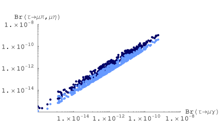
Figure 13: $Br(\tau\to\mu\pi)$ (dark-blue) and $Br(\tau\to\mu\eta)$ (light-blue) as functions of $Br(\tau\to\mu\gamma)$.

In Fig. 13 we show $Br(\tau\to\mu\pi)$ and $Br(\tau\to\mu\eta)$ as functions of $Br(\tau\to\mu\gamma)$, imposing the constraints from $\mu\to e\gamma$ and $\mu^{-}\to e^{-}e^{+}e^{-}$. We find that $Br(\tau\to\mu\pi)$ can reach values as high as $2\cdot 10^{-9}$ and $Br(\tau\to\mu\eta)$ can be as large as $7\cdot 10^{-10}$, which is still by more than one order of magnitude below the recent bounds from Belle and BaBar. We do not show $Br(\tau\to\mu\eta^{\prime})$ as it is very similar to $Br(\tau\to\mu\eta)$.

Completely analogous correlations can be found also for the corresponding decays $\tau\to e\pi,e\eta,e\eta^{\prime}$ and $\tau\to e\gamma$. Indeed, this symmetry between $\tau\to\mu$ and $\tau\to e$ systems turns out to be a general feature of the LHT model, that can be found in all decays considered in the present paper. We will return to this issue in Section 13.

An immediate consequence of these correlations is that, as in the case of $\tau\to\mu\gamma$ and $\tau\to e\gamma$, the highest values for $\tau\to\mu\pi$ are possible if $\tau\to e\pi$ is relatively small, and vice versa. Still the corresponding branching ratios can be simultaneously enhanced to $3\cdot 10^{-10}$. Analogous statements apply to $\tau\to\mu(e)\eta$ and $\tau\to\mu(e)\eta^{\prime}$.

12.6 $K_{L}\to\mu e$ and $K_{L}\to\pi^{0}\mu e$

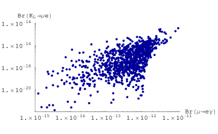
Figure 14: Correlation between $Br(\mu\to e\gamma)$ and $Br(K_{L}\to\mu e)$ for fixed mirror quark parameters $(m^{q}_{H1}\simeq 332\,{\rm GeV},m^{q}_{H2}\simeq 739\,{\rm GeV},m^{q}_{H3}\simeq 819\,{\rm GeV},\theta^{d}_{12}\simeq 95^{\circ},\theta^{d}_{13}\simeq 229^{\circ},\theta^{d}_{23}\simeq 205^{\circ},\delta^{d}_{12}=0,\delta^{d}_{13}\simeq 239^{\circ},\delta^{d}_{23}=0)$.

In Fig. 14 we show the dependence of $Br(K_{L}\to\mu e)$ on $Br(\mu\to e\gamma)$. To this end we have chosen one of the sets of mirror quark parameters for which the most spectacular effects both in $S_{\psi\phi}$ and the $K\to\pi\nu\bar{\nu}$ decays have been found [3]. We observe that for the parameters used here, $Br(K_{L}\to\mu e)$ is still by two orders of magnitude below the current experimental upper bound. However, one can see in Table 2 that $Br(K_{L}\to\mu e)$ could also be found only one order of magnitude below the current bound. This means that large effects in the $K\to\pi\nu\bar{\nu}$ decays do not necessarily imply also large effects in $K_{L}\to\mu e$.

The effects in $K_{L}\to\pi^{0}\mu e$ are even by roughly two orders of magnitude smaller, as can also be seen in Table 2, so that, from the point of view of the LHT model, this decay will not be observed in the foreseeable future.

12.7 Upper Bounds

In Table 2 we show the present LHT upper bounds on all branching ratios considered in the present paper, together with the corresponding experimental bounds. In order to see the strong dependence on the scale $f$, we give these bounds both for $f=1000\,{\rm GeV}$ and $f=500\,{\rm GeV}$ with the range (12.3) for the mirror lepton masses in both cases. We observe that the upper bounds on $\tau$ decays, except for $\tau^{-}\to\mu^{-}e^{+}\mu^{-}$ and $\tau^{-}\to e^{-}\mu^{+}e^{-}$ increase by almost two orders of magnitude, when lowering the scale $f$ down to $500\,{\rm GeV}$, so that these decays could be found close to their current experimental upper bounds. In particular, the most recent upper bounds on $\tau\to\mu\pi,e\pi$ [39] could be violated by roughly a factor 5, as can be seen from Table 2 of the first version of the present paper. Therefore, in deriving the LHT upper bounds for $f=500\,{\rm GeV}$, we have taken into account also the latter bounds. On the other hand, the bounds on $\tau^{-}\to\mu^{-}e^{+}\mu^{-}$ and $\tau^{-}\to e^{-}\mu^{+}e^{-}$ are quite independent of the value of $f$. This striking difference is due to the fact that the present lepton constraints are only effective for $\mu\to e$ transitions. We also note that the upper bounds on some $K$ and $B_{d,s}$ decays, namely $K_{L}\to\mu e$, $K_{L}\to\pi^{0}\mu e$ and $B_{d,s}\to\mu e$, result to be lower when the NP scale is decreased to $f=500\,{\rm GeV}$. The origin of this behaviour is that lowering $f$ the strongest constraints, mainly on $K$ and $B$ systems, start to exclude some range of parameters and, consequently, to forbid very large values for the branching ratios in question.

decay	$f=1000\,{\rm GeV}$	$f=500\,{\rm GeV}$	exp. upper bound
$\mu\to e\gamma$	$1.2\cdot 10^{-11}$ ($1\cdot 10^{-11}$)	$1.2\cdot 10^{-11}$ ($1\cdot 10^{-11}$)	$1.2\cdot 10^{-11}$ [23]
$\mu^{-}\to e^{-}e^{+}e^{-}$	$1.0\cdot 10^{-12}$ ($1\cdot 10^{-12}$)	$1.0\cdot 10^{-12}$ ($1\cdot 10^{-12}$)	$1.0\cdot 10^{-12}$ [48]
$\mu\text{Ti}\to e\text{Ti}$	$2\cdot 10^{-10}$ ($5\cdot 10^{-12}$)	$4\cdot 10^{-11}$ ($5\cdot 10^{-12}$)	$4.3\cdot 10^{-12}$ [35]
$\tau\to e\gamma$	$8\cdot 10^{-10}$ ($7\cdot 10^{-10}$)	${1\cdot 10^{-8}}$ (${1\cdot 10^{-8}}$)	${9.4\cdot 10^{-8}}$ [39]
$\tau\to\mu\gamma$	$8\cdot 10^{-10}$ ($8\cdot 10^{-10}$)	$2\cdot 10^{-8}$ (${1\cdot 10^{-8}}$)	${1.6\cdot 10^{-8}}$ [39]
$\tau^{-}\to e^{-}e^{+}e^{-}$	$7\cdot 10^{-10}$ ($6\cdot 10^{-10}$)	${2\cdot 10^{-8}}$ (${2\cdot 10^{-8}}$)	$2.0\cdot 10^{-7}$ [77]
$\tau^{-}\to\mu^{-}\mu^{+}\mu^{-}$	$7\cdot 10^{-10}$ ($6\cdot 10^{-10}$)	${3\cdot 10^{-8}}$ (${3\cdot 10^{-8}}$)	$1.9\cdot 10^{-7}$ [77]
$\tau^{-}\to e^{-}\mu^{+}\mu^{-}$	$5\cdot 10^{-10}$ ($5\cdot 10^{-10}$)	${2\cdot 10^{-8}}$ (${2\cdot 10^{-8}}$)	$2.0\cdot 10^{-7}$ [78]
$\tau^{-}\to\mu^{-}e^{+}e^{-}$	$5\cdot 10^{-10}$ ($5\cdot 10^{-10}$)	${2\cdot 10^{-8}}$ (${2\cdot 10^{-8}}$)	$1.9\cdot 10^{-7}$ [78]
$\tau^{-}\to\mu^{-}e^{+}\mu^{-}$	$5\cdot 10^{-14}$ ($3\cdot 10^{-14}$)	${2\cdot 10^{-14}}$ (${2\cdot 10^{-14}}$)	$1.3\cdot 10^{-7}$ [77]
$\tau^{-}\to e^{-}\mu^{+}e^{-}$	$5\cdot 10^{-14}$ ($3\cdot 10^{-14}$)	${2\cdot 10^{-14}}$ (${2\cdot 10^{-14}}$)	$1.1\cdot 10^{-7}$ [77]
$\tau\to\mu\pi$	$2\cdot 10^{-9}$ ($2\cdot 10^{-9}$)	${5.8\cdot 10^{-8}}$ (${5.8\cdot 10^{-8}}$)	${5.8\cdot 10^{-8}}$ [39]
$\tau\to e\pi$	$2\cdot 10^{-9}$ ($2\cdot 10^{-9}$)	${4.4\cdot 10^{-8}}$ (${4.4\cdot 10^{-8}}$)	${4.4\cdot 10^{-8}}$ [39]
$\tau\to\mu\eta$	$6\cdot 10^{-10}$ $(6\cdot 10^{-10})$	${2\cdot 10^{-8}}$ ${(2\cdot 10^{-8})}$	${5.1\cdot 10^{-8}}$ [39]
$\tau\to e\eta$	$6\cdot 10^{-10}$ $(6\cdot 10^{-10})$	${2\cdot 10^{-8}}$ ${(2\cdot 10^{-8})}$	${4.5\cdot 10^{-8}}$ [39]
$\tau\to\mu\eta^{\prime}$	$7\cdot 10^{-10}$ $(7\cdot 10^{-10})$	${3\cdot 10^{-8}}$ ${(3\cdot 10^{-8})}$	${5.3\cdot 10^{-8}}$ [39]
$\tau\to e\eta^{\prime}$	$7\cdot 10^{-10}$ $(7\cdot 10^{-10})$	${3\cdot 10^{-8}}$ ${(3\cdot 10^{-8})}$	${9.0\cdot 10^{-8}}$ [39]
$K_{L}\to\mu e$	$4\cdot 10^{-13}$ ($2\cdot 10^{-13}$)	$3\cdot 10^{-14}$ ($3\cdot 10^{-14}$)	$4.7\cdot 10^{-12}$ [56]
$K_{L}\to\pi^{0}\mu e$	$4\cdot 10^{-15}$ ($2\cdot 10^{-15}$)	$5\cdot 10^{-16}$ ($5\cdot 10^{-16}$)	$6.2\cdot 10^{-9}$ [79]
$B_{d}\to\mu e$	$5\cdot 10^{-16}$ ($2\cdot 10^{-16}$)	$9\cdot 10^{-17}$ ($9\cdot 10^{-17}$)	$1.7\cdot 10^{-7}$ [80]
$B_{s}\to\mu e$	$5\cdot 10^{-15}$ ($2\cdot 10^{-15}$)	$9\cdot 10^{-16}$ ($9\cdot 10^{-16}$)	$6.1\cdot 10^{-6}$ [81]
$B_{d}\to\tau e$	$3\cdot 10^{-11}$ ($2\cdot 10^{-11}$)	${2\cdot 10^{-10}}$ ($2\cdot 10^{-10}$)	$1.1\cdot 10^{-4}$ [82]
$B_{s}\to\tau e$	$2\cdot 10^{-10}$ ($2\cdot 10^{-10}$)	${2\cdot 10^{-9}}$ ($2\cdot 10^{-9}$)	—
$B_{d}\to\tau\mu$	$3\cdot 10^{-11}$ ($3\cdot 10^{-11}$)	$3\cdot 10^{-10}$ ($3\cdot 10^{-10}$)	$3.8\cdot 10^{-5}$ [82]
$B_{s}\to\tau\mu$	$2\cdot 10^{-10}$ ($2\cdot 10^{-10}$)	$3\cdot 10^{-9}$ ($3\cdot 10^{-9}$)	—

Table 2: Upper bounds on LFV decay branching ratios in the LHT model, for two different values of the scale $f$, after imposing the constraints on $\mu\to e\gamma$ and $\mu^{-}\to e^{-}e^{+}e^{-}$. The numbers given in brackets are obtained after imposing the additional constraint $R(\mu\text{Ti}\to e\text{Ti})<5\cdot 10^{-12}$. For $f=500\,{\rm GeV}$, also the bounds on $\tau\to\mu\pi,e\pi$ have been included. The current experimental upper bounds are also given.

We have also investigated the effect of imposing in addition the constraint $R(\mu\text{Ti}\to e\text{Ti})<5\cdot 10^{-12}$, which we choose slightly above the experimental value $4.3\cdot 10^{-12}$ in order to account for the theoretical uncertainties involved. We find that all upper bounds collected in Table 2 depend only weakly on that constraint. This finding justifies that we did not take into account this bound in our numerical analysis so far, as it has only a minor impact on the observables discussed.

We would like to stress that the bounds in Table 2 should only be considered as rough upper bounds. They have been obtained from scattering over the allowed parameter space of the model. In particular, no confidence level can be assigned to them. The same applies to the ranges given in Table 3 for the LHT model.

12.8 $(g-2)_{\mu}$

Finally, we have analyzed $(g-2)_{\mu}$ in the LHT model. Even for the scale $f$ being as low as $500\,{\rm GeV}$, we find

$$a_{\mu}^{\text{LHT}}<1.2\cdot 10^{-10}\,,$$ (12.7)

to be compared with the experimental value in (11.1). We observe that the effect of mirror fermions is by roughly a factor of 5 below the current experimental uncertainty, implying that the possible discrepancy between the SM value and the data cannot be solved in the model considered here.

13 Patterns of Correlations and Comparison with Supersymmetry

13.1 Preliminaries

We have seen in the previous section that the branching ratios for several charged LFV processes could reach within the LHT model the level accessible to experiments performed in this decade. However, in view of many parameters involved, it is desirable to look for certain correlations between various branching ratios that are less parameter dependent than individual branching ratios, and whose pattern could provide a clear signature of the LHT model.

In the case of CMFV in the quark sector useful correlations have been summarized at length in [22, 83]. In the case of LFV, in a very interesting paper [29], Ellis et al. noticed a number of correlations characteristic for the MSSM, in the absence of significant Higgs contributions. These correlations have also been analyzed recently in [30, 31, 32]. In particular, in [30, 32] modifications of them in the presence of significant Higgs contributions have been pointed out.

The main goal of this section is a brief review of the correlations discussed in [29, 30, 31, 32] and the comparison of MSSM results with the ones of the LHT model. We will see that indeed the correlations in question could allow for a transparent distinction between MSSM and LHT, which is difficult in high energy collider processes [84].

13.2 Correlations in the MSSM

13.2.1 Dipole Operator Dominance

In the absence of significant Higgs boson contributions, the LFV processes considered in our paper are dominated in the MSSM by the dipole operator with very small contributions from box and $Z$-penguin diagrams. In this case one finds the approximate general formulae [29, 30, 31, 32]

$$\frac{Br(\ell_{i}^{-}\to\ell_{j}^{-}\ell_{j}^{+}\ell_{j}^{-})}{Br(\ell_{i}\to\ell_{j}\gamma)} \simeq \frac{\alpha}{3\pi}\left(\log\frac{m_{\ell_{i}}^{2}}{m_{\ell_{j}}^{2}}-2.7\right)\,,$$ (13.1)

$$\frac{Br(\ell_{i}^{-}\to\ell_{j}^{-}\ell_{k}^{+}\ell_{k}^{-})}{Br(\ell_{i}\to\ell_{j}\gamma)} \simeq \frac{\alpha}{3\pi}\left(\log\frac{m_{\ell_{i}}^{2}}{m_{\ell_{k}}^{2}}-2.7\right)\,.$$ (13.2)

Consequently one finds

$$\frac{Br(\mu^{-}\to e^{-}e^{+}e^{-})}{Br(\mu\to e\gamma)} \simeq \frac{\alpha}{3\pi}\left(\log\frac{m_{\mu}^{2}}{m_{e}^{2}}-2.7\right)\simeq\frac{1}{162}\,,\qquad$$ (13.3)

$$\frac{Br(\tau^{-}\to e^{-}e^{+}e^{-})}{Br(\tau\to e\gamma)}\simeq\frac{Br(\tau^{-}\to\mu^{-}e^{+}e^{-})}{Br(\tau\to\mu\gamma)} \simeq \frac{\alpha}{3\pi}\left(\log\frac{m_{\tau}^{2}}{m_{e}^{2}}-2.7\right)\simeq\frac{1}{95}\,,$$ (13.4)

$$\frac{Br(\tau^{-}\to\mu^{-}\mu^{+}\mu^{-})}{Br(\tau\to\mu\gamma)}\simeq\frac{Br(\tau^{-}\to e^{-}\mu^{+}\mu^{-})}{Br(\tau\to e\gamma)} \simeq \frac{\alpha}{3\pi}\left(\log\frac{m_{\tau}^{2}}{m_{\mu}^{2}}-2.7\right)\simeq\frac{1}{438}\,,$$ (13.5)

and [32]

$$\frac{Br(\tau^{-}\to\mu^{-}e^{+}e^{-})}{Br(\tau^{-}\to\mu^{-}\mu^{+}\mu^{-})}\simeq\frac{Br(\tau^{-}\to e^{-}e^{+}e^{-})}{Br(\tau^{-}\to e^{-}\mu^{+}\mu^{-})}\simeq 4.6\,.$$ (13.6)

Moreover, keeping only the dipole operator contribution in $R(\mu\text{Ti}\to e\text{Ti})$, we find

$$\frac{R(\mu\text{Ti}\to e\text{Ti})}{Br(\mu\to e\gamma)}\simeq 0.7\alpha\,.$$ (13.7)

One also has

$$\frac{Br(\tau\to\ell P)}{Br(\tau\to\ell\gamma)}<{\cal O}(\alpha)\qquad(P=\pi,\eta,\eta^{\prime})\,,$$ (13.8)

where the absence of dipole operator contributions to $Br(\tau\to\ell P)$ makes the ratios in (13.8) significantly smaller than the ones in (13.3)–(13.5).

13.2.2 Including Higgs Contributions: Decoupling Limit

It should be emphasized that the Higgs contributions become competitive with the gauge mediated ones, once the Higgs masses are roughly by one order of magnitude smaller than the sfermion masses and $\tan\beta$ is ${\cal O}(40-50)$. There is a rich literature on Higgs contributions to LFV within supersymmetry. One of the earlier references is the one by Babu and Kolda [85]. Here we concentrate on the modifications of the correlations discussed above in the presence of significant Higgs contributions as analyzed by Paradisi [32], where further references can be found (see in particular [30]).

In the limit of Higgs decoupling, which is achieved in the MSSM, some of the results in (13.1)–(13.8) are modified. In particular

$$\frac{Br(\tau^{-}\to\mu^{-}\mu^{+}\mu^{-})}{Br(\tau\to\mu\gamma)}\mathrel{\hbox to0.0pt{\raise 2.20013pt\hbox{$<$}\hss}{\lower 2.20013pt\hbox{$\sim$}}}\frac{2}{9}\,,\qquad\frac{Br(\tau^{-}\to e^{-}\mu^{+}\mu^{-})}{Br(\tau\to e\gamma)}\mathrel{\hbox to0.0pt{\raise 2.20013pt\hbox{$<$}\hss}{\lower 2.20013pt\hbox{$\sim$}}}\frac{1}{12}$$ (13.9)

can be much larger than in the case of dipole operator dominance, and

$$\frac{Br(\tau^{-}\to\mu^{-}e^{+}e^{-})}{Br(\tau^{-}\to\mu^{-}\mu^{+}\mu^{-})}\mathrel{\hbox to0.0pt{\raise 2.20013pt\hbox{$>$}\hss}{\lower 2.20013pt\hbox{$\sim$}}}0.05\,,\qquad\frac{Br(\tau^{-}\to e^{-}e^{+}e^{-})}{Br(\tau^{-}\to e^{-}\mu^{+}\mu^{-})}\mathrel{\hbox to0.0pt{\raise 2.20013pt\hbox{$>$}\hss}{\lower 2.20013pt\hbox{$\sim$}}}0.13$$ (13.10)

can be much smaller. Moreover one finds

$$\frac{Br(\tau\to\ell\eta)}{Br(\tau\to\ell\gamma)}\mathrel{\hbox to0.0pt{\raise 2.20013pt\hbox{$<$}\hss}{\lower 2.20013pt\hbox{$\sim$}}}1\,,\qquad\frac{Br(\tau\to\mu\eta)}{Br(\tau^{-}\to\mu^{-}\mu^{+}\mu^{-})}\simeq 4.5\,,\qquad\frac{Br(\tau\to e\eta)}{Br(\tau^{-}\to e^{-}\mu^{+}\mu^{-})}\simeq 12\,.$$ (13.11)

13.3 Correlations in the LHT Model

The pattern of correlations in the LHT model differs significantly from the MSSM one presented above. This is due to the fact that the dipole contributions to the decays $\ell_{i}^{-}\to\ell_{j}^{-}\ell_{j}^{+}\ell_{j}^{-}$ and $\ell_{i}^{-}\to\ell_{j}^{-}\ell_{k}^{+}\ell_{k}^{-}$ can be fully neglected in comparison with $Z^{0}$-penguin and box diagram contributions. This is dominantly due to the fact that the neutral gauge boson $(Z_{H},A_{H})$ contributions interfere destructively with the $W_{H}^{\pm}$ contributions to the dipole operator functions $\bar{D}^{\prime\,ij}_{\text{odd}}$, but constructively in the case of the functions $\bar{Y}^{ij}_{k,\text{odd}}$ that summarize the $Z^{0}$-penguin and box contributions in a gauge independent manner. Moreover, the large $\tan\beta$ enhancement of dipole operators characteristic for the MSSM is absent here. In this context it is useful to define the ratios

$$T_{ij}=\left|\frac{\bar{Y}^{ij}_{j,\text{odd}}}{\bar{D}^{\prime\,ij}_{\text{odd}}}\right|^{2}$$ (13.12)

that are strongly enhanced in the case of the LHT model for almost the entire space of parameters, as seen in Fig. 15 for the case of $T_{\mu e}$. Consequently, the logarithmic enhancement of dipole contributions seen in (5.8), (13.1) and (13.2) is eliminated by the strong suppression of $|\bar{D}^{\prime\,ij}_{\text{odd}}|^{2}$ with respect to $|\bar{Y}^{ij}_{j,\text{odd}}|^{2}$. Similarly, $C_{7}^{\tau\mu}$, that is governed by $\bar{D}^{\prime\,\tau\mu}_{\text{odd}}$, can be neglected in (10.10), resulting in the absence of large logarithms in the decays $\tau^{-}\to\mu^{-}e^{+}e^{-}$ and $\tau^{-}\to e^{-}\mu^{+}\mu^{-}$.

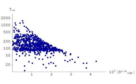
Figure 15: $T_{\mu e}$ as a function of $|\bar{D}^{\prime\,\mu e}_{\text{odd}}|$ for $f=1\,{\rm TeV}$.

We note that the ratios $T_{ij}$ depend on the approximation made for the left-over singularity, as $\bar{Y}^{ij}_{j,\text{odd}}$ suffers from this divergence while $\bar{D}^{{}^{\prime}\,ij}_{\text{odd}}$ does not. However, we find that dropping completely the term proportional to $S_{\text{odd}}$, which is certainly not a good approximation, amounts to at most 50% changes in the allowed ranges for $T_{ij}$ and consequently for the correlations discussed below. Therefore we think that these correlations are only insignificantly affected by this general feature of non-linear sigma models.

These findings make clear that the correlations between various branching ratios in the LHT model, being unaffected by the logarithms present in (13.1)–(13.5), have a very different pattern from those found in the MSSM.

It turns out that within an accuracy of $3\%$ one can set $\bar{D}^{\prime\,ij}_{\text{odd}}$ to zero in all decays with three leptons in the final state. Similarly, the contribution of $\tilde{C}_{9}^{ij}$ in $\tau^{-}\to\mu^{-}e^{+}e^{-}$ and $\tau^{-}\to e^{-}\mu^{+}\mu^{-}$ can be neglected. Neglecting finally $\Delta_{ij}$ in (10.6), which is good to within 20%, allows us to derive simple expressions for various ratios of branching ratios that can directly be compared with those listed in (13.1)–(13.6).

To this end, we define

$$a_{ij}=\frac{\bar{Z}^{ij}_{\text{odd}}}{\bar{Y}^{ij}_{j,\text{odd}}}\,,\qquad b^{k}_{ij}=\left|\frac{\bar{Y}^{ij}_{k,\text{odd}}}{\bar{Y}^{ij}_{j,\text{odd}}}\right|^{2}\,,$$ (13.13)

$$c_{ij}=3\sin^{4}\theta_{W}|a_{ij}|^{2}+\frac{1}{2}-2\sin^{2}\theta_{W}\text{Re}{(a_{ij})}\,.$$ (13.14)

We find then

$$\frac{Br(\mu^{-}\to e^{-}e^{+}e^{-})}{Br(\mu\to e\gamma)}\simeq\frac{2\alpha}{3\pi}\frac{1}{\sin^{4}\theta_{W}}T_{\mu e}c_{\mu e}\,,$$ (13.15)

with analogous expressions for the respective $\tau\to e$ and $\tau\to\mu$ transitions.

We also find

$$\frac{Br(\tau^{-}\to e^{-}\mu^{+}\mu^{-})}{Br(\tau\to e\gamma)} \simeq \frac{\alpha}{12\pi}\frac{1}{\sin^{4}\theta_{W}}T_{\tau e}b^{\mu}_{\tau e}\,.$$ (13.16)

$$\frac{Br(\tau^{-}\to\mu^{-}e^{+}e^{-})}{Br(\tau\to\mu\gamma)} \simeq \frac{\alpha}{12\pi}\frac{1}{\sin^{4}\theta_{W}}T_{\tau\mu}b^{e}_{\tau\mu}\,,$$ (13.17)

Finally, (13.15)–(13.17) imply

$$\frac{Br(\tau^{-}\to e^{-}e^{+}e^{-})}{Br(\tau^{-}\to e^{-}\mu^{+}\mu^{-})} = 8\frac{c_{\tau e}}{b^{\mu}_{\tau e}}\,,$$ (13.18)

$$\frac{Br(\tau^{-}\to\mu^{-}\mu^{+}\mu^{-})}{Br(\tau^{-}\to\mu^{-}e^{+}e^{-})} = 8\frac{c_{\tau\mu}}{b^{e}_{\tau\mu}}\,.$$ (13.19)

In what follows we restrict ourselves to $f=1\,{\rm TeV}$ for simplicity. We note that although the numerical values given below depend slightly on the size of the scale $f$, the qualitative picture found and discussed remains true independently of that value.

The ranges for the ratios in question found in the LHT model are compared in Table 3 with the corresponding values in the MSSM, both in the case of dipole dominance and when Higgs contributions are significant.

ratio	LHT	MSSM (dipole)	MSSM (Higgs)
$\frac{Br(\mu^{-}\to e^{-}e^{+}e^{-})}{Br(\mu\to e\gamma)}$	0.4…2.5	$\sim 6\cdot 10^{-3}$	$\sim 6\cdot 10^{-3}$
$\frac{Br(\tau^{-}\to e^{-}e^{+}e^{-})}{Br(\tau\to e\gamma)}$	0.4…2.3	$\sim 1\cdot 10^{-2}$	${\sim 1\cdot 10^{-2}}$
$\frac{Br(\tau^{-}\to\mu^{-}\mu^{+}\mu^{-})}{Br(\tau\to\mu\gamma)}$	0.4…2.3	$\sim 2\cdot 10^{-3}$	$0.06\dots 0.1$
$\frac{Br(\tau^{-}\to e^{-}\mu^{+}\mu^{-})}{Br(\tau\to e\gamma)}$	0.3…1.6	$\sim 2\cdot 10^{-3}$	$0.02\dots 0.04$
$\frac{Br(\tau^{-}\to\mu^{-}e^{+}e^{-})}{Br(\tau\to\mu\gamma)}$	0.3…1.6	$\sim 1\cdot 10^{-2}$	${\sim 1\cdot 10^{-2}}$
$\frac{Br(\tau^{-}\to e^{-}e^{+}e^{-})}{Br(\tau^{-}\to e^{-}\mu^{+}\mu^{-})}$	1.3…1.7	$\sim 5$	0.3…0.5
$\frac{Br(\tau^{-}\to\mu^{-}\mu^{+}\mu^{-})}{Br(\tau^{-}\to\mu^{-}e^{+}e^{-})}$	1.2…1.6	$\sim 0.2$	5…10
$\frac{R(\mu\text{Ti}\to e\text{Ti})}{Br(\mu\to e\gamma)}$	$10^{-2}\dots 10^{2}$	$\sim 5\cdot 10^{-3}$	$0.08\dots 0.15$

Table 3: Comparison of various ratios of branching ratios in the LHT model and in the MSSM without and with significant Higgs contributions.

While the results in Table 3 are self-explanatory, let us emphasize four striking differences between the LHT and MSSM results in the case of small Higgs contributions:

• The ratio (13.15) and the similar ratios for $\tau\to e$ and $\tau\to\mu$ transitions are ${\cal O}(1)$ in the LHT model as opposed to ${\cal O}(\alpha)$ in the MSSM.

• Also the $\mu-e$ conversion rate in nuclei, normalized to $Br(\mu\to e\gamma)$, can be significantly enhanced in the LHT model, with respect to the MSSM without significant Higgs contributions. However the distinction in this case is not as clear as in the case of $Br(\ell_{i}^{-}\to\ell_{j}^{-}\ell_{j}^{+}\ell_{j}^{-})/Br(\ell_{i}\to\ell_{j}\gamma)$ due to a destructive interference of the different contributions to $\mu-e$ conversion (see (6.2)). On the other hand, in the case of the MSSM with significant Higgs contributions, $R(\mu\text{Ti}\to e\text{Ti})/Br(\mu\to e\gamma)$ is typically much larger than $\alpha$, so that a distinction from the LHT model would be difficult in that case.

• The “inverted” pattern of the ratios in (13.6) is absent in the LHT model as the ratios (13.18) and (13.19) are comparable in magnitude. Moreover they are generally very different from the MSSM values.

• The last finding also implies that while the ratios (13.4) and (13.5) differ roughly by a factor of 5 in the case of the MSSM, they are comparable in the LHT model, as seen in (13.16) and (13.17).

In order to exhibit these different patterns in a transparent manner, let us define the three ratios

$$R_{1} = \frac{Br(\tau^{-}\to e^{-}e^{+}e^{-})}{Br(\tau^{-}\to\mu^{-}\mu^{+}\mu^{-})}\frac{Br(\tau^{-}\to\mu^{-}e^{+}e^{-})}{Br(\tau^{-}\to e^{-}\mu^{+}\mu^{-})}\,,$$ (13.20)

$$R_{2} = \frac{Br(\tau^{-}\to e^{-}e^{+}e^{-})}{Br(\tau^{-}\to\mu^{-}\mu^{+}\mu^{-})}\frac{Br(\tau\to\mu\gamma)}{Br(\tau\to e\gamma)}\,,$$ (13.21)

$$R_{3} = \frac{Br(\tau^{-}\to e^{-}\mu^{+}\mu^{-})}{Br(\tau^{-}\to\mu^{-}e^{+}e^{-})}\frac{Br(\tau\to\mu\gamma)}{Br(\tau\to e\gamma)}\,.$$ (13.22)

Note that in the case of a $\mu\leftrightarrow e$ symmetry, these three ratios should be equal to unity. This symmetry is clearly very strongly broken in the MSSM, due to the sensitivity of the ratios in (13.1) and (13.2) to $m_{e}$ and $m_{\mu}$, where one finds

$$R_{1}\simeq{20}\,,\qquad R_{2}\simeq{5}\,,\qquad R_{3}\simeq 0.2\qquad\text{(MSSM)}\,.$$ (13.23)

On the other hand, in the case of the LHT model the absence of large logarithms allows to satisfy the $\mu\leftrightarrow e$ symmetry in question within 30%, so that we find

$$0.8\mathrel{\hbox to0.0pt{\raise 2.20013pt\hbox{$<$}\hss}{\lower 2.20013pt\hbox{$\sim$}}}R_{1}\mathrel{\hbox to0.0pt{\raise 2.20013pt\hbox{$<$}\hss}{\lower 2.20013pt\hbox{$\sim$}}}1.3\,,\qquad 0.8\mathrel{\hbox to0.0pt{\raise 2.20013pt\hbox{$<$}\hss}{\lower 2.20013pt\hbox{$\sim$}}}R_{2}\mathrel{\hbox to0.0pt{\raise 2.20013pt\hbox{$<$}\hss}{\lower 2.20013pt\hbox{$\sim$}}}1.2\,,\qquad 0.8\mathrel{\hbox to0.0pt{\raise 2.20013pt\hbox{$<$}\hss}{\lower 2.20013pt\hbox{$\sim$}}}R_{3}\mathrel{\hbox to0.0pt{\raise 2.20013pt\hbox{$<$}\hss}{\lower 2.20013pt\hbox{$\sim$}}}1.2\qquad\text{(LHT)}\,.$$ (13.24)

The comparison of (13.23) with (13.24) offers a very clear distinction between these two models.

In the presence of significant Higgs contributions the distinction between MSSM and LHT is less pronounced in $\tau$ decays with $\mu$ in the final state. However even in this case both models can be distinguished, as seen in Table 3. In particular, the four ratios involving $Br(\ell_{i}\to\ell_{j}\gamma)$ are still significantly smaller in the MSSM than in the LHT model, and all decays with electrons in the final state offer excellent means to distinguish these two models.

For the decays $\tau\to\ell P$ with $P=\pi,\eta,\eta^{\prime}$ we find the ranges

$$1\mathrel{\hbox to0.0pt{\raise 2.20013pt\hbox{$<$}\hss}{\lower 2.20013pt\hbox{$\sim$}}}\frac{Br(\tau\to\ell\pi)}{Br(\tau\to\ell\gamma)}\mathrel{\hbox to0.0pt{\raise 2.20013pt\hbox{$<$}\hss}{\lower 2.20013pt\hbox{$\sim$}}}5.5\,,\qquad 0.4\mathrel{\hbox to0.0pt{\raise 2.20013pt\hbox{$<$}\hss}{\lower 2.20013pt\hbox{$\sim$}}}\frac{Br(\tau\to\ell\eta)}{Br(\tau\to\ell\gamma)}\mathrel{\hbox to0.0pt{\raise 2.20013pt\hbox{$<$}\hss}{\lower 2.20013pt\hbox{$\sim$}}}2\,,\qquad 0.3\mathrel{\hbox to0.0pt{\raise 2.20013pt\hbox{$<$}\hss}{\lower 2.20013pt\hbox{$\sim$}}}\frac{Br(\tau\to\ell\eta^{\prime})}{Br(\tau\to\ell\gamma)}\mathrel{\hbox to0.0pt{\raise 2.20013pt\hbox{$<$}\hss}{\lower 2.20013pt\hbox{$\sim$}}}2.8\,.$$ (13.25)

As seen in (13.8), the ratios obtained in the LHT model are much larger than in supersymmetry without significant Higgs contributions. On the other hand, if the Higgs contributions are dominant, the distinction through the first inequality of (13.11) will be difficult. However, we also find

$$0.7\mathrel{\hbox to0.0pt{\raise 2.20013pt\hbox{$<$}\hss}{\lower 2.20013pt\hbox{$\sim$}}}\frac{Br(\tau\to\mu\eta)}{Br(\tau^{-}\to\mu^{-}\mu^{+}\mu^{-})}\mathrel{\hbox to0.0pt{\raise 2.20013pt\hbox{$<$}\hss}{\lower 2.20013pt\hbox{$\sim$}}}1.3\,,\qquad 1.1\mathrel{\hbox to0.0pt{\raise 2.20013pt\hbox{$<$}\hss}{\lower 2.20013pt\hbox{$\sim$}}}\frac{Br(\tau\to e\eta)}{Br(\tau^{-}\to e^{-}\mu^{+}\mu^{-})}\mathrel{\hbox to0.0pt{\raise 2.20013pt\hbox{$<$}\hss}{\lower 2.20013pt\hbox{$\sim$}}}1.8\,,$$ (13.26)

that could be distinguished from the corresponding results in (13.11).

In summary we have demonstrated that the LHT model can be very transparently distinguished from the MSSM with the help of LFV processes, while such a distinction is non-trivial in the case of high energy processes [84]. We consider this result as one of the most interesting ones of our paper.

14 Conclusions

In the present paper we have extended our analysis of flavour and CP-violating processes in the LHT model [14, 3] to the lepton sector.

In contrast to rare $K$ and $B$ decays, where the SM contributions play an important and often the dominant role in the LHT model, the smallness of ordinary neutrino masses assures that the mirror fermion contributions to LFV processes are by far the dominant effects. Moreover, the absence of QCD corrections and hadronic matrix elements allows in most cases to make predictions entirely within perturbation theory. Exceptions are the decays $B_{d,s}\to\ell_{i}\ell_{j}$ that involve the weak decay constants $F_{B_{d,s}}$.

The decays and transitions considered by us can be divided into two broad classes: those which suffer from some sensitivity to the UV completion signalled by the logarithmic dependence on the cut-off (class A) and those which are free from this dependence (class B). We have

Class A

$$\mu^{-}\to e^{-}e^{+}e^{-}\,,\qquad\tau^{-}\to e^{-}e^{+}e^{-}\,,\qquad\tau^{-}\to\mu^{-}\mu^{+}\mu^{-}\,,\qquad\mu\to e\text{ conversion}\,,$$

$$\tau^{-}\to\mu^{-}e^{+}e^{-}\,,\qquad\tau^{-}\to e^{-}\mu^{+}\mu^{-}\,,\qquad{\tau\to\mu(e)\pi\,,\qquad\tau\to\mu(e)\eta\,,\qquad\tau\to\mu(e)\eta^{\prime}}\,.$$

Class B

$$\mu\to e\gamma\,,\qquad\tau\to e\gamma\,,\qquad\tau\to\mu\gamma\,,$$

$$K_{L,S}\to\mu e\,,\qquad K_{L,S}\to\pi^{0}\mu e\,,\qquad B_{d,s}\to\mu e\,,\qquad B_{d,s}\to\tau e\qquad B_{d,s}\to\tau\mu\,,$$

$$\tau^{-}\to e^{-}\mu^{+}e^{-}\,,\qquad\tau^{-}\to\mu^{-}e^{+}\mu^{-}\,,\qquad(g-2)_{\mu}\,.$$

Clearly the predictions for the decays in class B are more reliable, but we believe that also our estimates of the rates of class A decays give at least correct orders of magnitude. Moreover, as pointed out in [3], the logarithmic divergence in question has a universal character and can simply be parameterized by a single parameter $\delta_{\text{div}}$ that one can in principle fit to the data and trade for one observable. At present this is not feasible, but could become realistic when more data for FCNC processes will be available. This reasoning assumes that $\delta_{\text{div}}$ encloses all effects coming from the UV completion, which is true if light fermions do not have a more complex relation to the fundamental fermions of the UV completion, that could spoil its flavour independence.

Bearing this in mind the main messages of our paper are as follows:

• As seen in Table 2, several rates considered by us can reach the present experimental upper bounds, and are very interesting in view of new experiments taking place in this decade. In fact, in order to suppress the $\mu\to e\gamma$ and $\mu^{-}\to e^{-}e^{+}e^{-}$ decay rates and the $\mu-e$ conversion rate in nuclei below the present experimental upper bounds, the relevant mixing matrix in the mirror lepton sector, $V_{H\ell}$, must be rather hierarchical, unless the spectrum of mirror leptons is quasi-degenerate.

• The correlations between various branching ratios analyzed in detail in Section 13 should allow a clear distinction of the LHT model from the MSSM. While in the MSSM without significant Higgs contributions the dominant role in decays with three leptons in the final state and in $\mu-e$ conversion in nuclei is played by the dipole operator, this operator is basically irrelevant in the LHT model, where $Z^{0}$-penguin and box diagram contributions are much more important. While in the Higgs mediated case, the distinction of the MSSM from the LHT model is less pronounced, all ratios involving $\ell_{i}\to\ell_{j}\gamma$ and in particular decays with electrons in the final state still offer excellent means to distinguish these two models.

• The measurements of all rates considered in the present paper should allow the full determination of the matrix $V_{H\ell}$, provided the masses of the mirror fermions and of the new heavy gauge bosons will be measured at the LHC.

• We point out that the measurements of $Br(K_{L}\to\mu e)$ and $Br(K_{L}\to\pi^{0}\mu e)$ will transparently shed some light on the complex phases present in the mirror quark sector.

• The contribution of mirror leptons to $(g-2)_{\mu}$ is negligible. This should also be contrasted with the MSSM with large $\tan\beta$ and not too heavy scalars, where those corrections could be significant, thus allowing to solve the possible discrepancy between SM prediction and experimental data [69].

• Another possibility to distinguish different NP models through LFV processes is given by the measurement of $\mu\to e\gamma$ with polarized muons. Measuring the angular distribution of the outgoing electrons, one can determine the size of left- and right-handed contributions separately [86]. In addition, detecting also the electron spin would yield information on the relative phase between these two contributions [87]. We recall that the LHT model is peculiar in this respect as it does not involve any right-handed contribution.

• It will be interesting to watch the experimental progress in LFV in the coming years with the hope to see some spectacular effects of mirror fermions in LFV decays that in the SM are basically unmeasurable. The correlations between various branching ratios analyzed in detail in Section 13 should be very useful in distinguishing the LHT model from other models, in particular the MSSM. In fact, this distinction should be easier than through high-energy processes at LHC, as LFV processes are theoretically very clean.

The decays $\mu\to e\gamma$, $\tau\to\mu\pi$ and $(g-2)_{\mu}$ have already been analyzed in the LHT model in [26, 27]. While we agree with these papers that mirror lepton effects in $\mu\to e\gamma$ and $\tau\to\mu\pi$ can be very large and are very small in $(g-2)_{\mu}$, we disagree at the quantitative level, as discussed in the text.

Acknowledgements

Our particular thanks go to Stefan Recksiegel for providing us the mirror quark parameters necessary for the study of the $K$ and $B_{d,s}$ decays, and to Paride Paradisi for very informative discussions on his work. We would also like to thank Wolfgang Altmannshofer, Gerhard Buchalla, Vincenzo Cirigliano, Andrzej Czarnecki and Michael Wick for useful discussions. This research was partially supported by the Cluster of Excellence ‘Origin and Structure of the Universe’ and by the German ‘Bundesministerium für Bildung und Forschung’ under contract 05HT6WOA.

Appendix A Neutrino Masses in the LHT Model

Within the LH model without T-parity, there have been several suggestions how to naturally explain the smallness of neutrino masses within the low-energy framework of the model [88, 89, 90, 91]. Although differing in the details, they are all based on a coupling of the form

$$Y_{ij}(L^{i})^{T}\Phi\mathcal{C}^{-1}L^{j}+h.c.\,,$$ (A.1)

where $L^{i}$ are the left-handed SM lepton doublets and $\mathcal{C}$ is the charge conjugation operator. This term violates lepton number by $\Delta L=2$ and generates Majorana masses for the left-handed neutrinos of size

$$m_{ij}=Y_{ij}v^{\prime}\,,$$ (A.2)

with $v^{\prime}$ being the VEV of the scalar triplet $\Phi$.

Thus, in order to explain the observed smallness of neutrino masses, either $Y_{ij}$ or $v^{\prime}/v$ has to be of ${\cal O}(10^{-11})$. While in the case of $Y_{ij}$, this appears to be an extremely fine-tuned scenario, in the case of $v^{\prime}$ some so far unknown mechanism could be at work that ensures the smallness of $v^{\prime}$. Such a mechanism would also be very welcome from the point of view of electroweak precision observables.

Indeed, (A.1) is a concrete example for the general mechanism found and discussed in [92] to generate Majorana neutrino masses for the left-handed neutrinos through their interaction with a triplet scalar field.

One should however be aware of the fact that (A.1) explicitly breaks the enlarged $[SU(2)\times U(1)]^{2}$ gauge symmetry of the LH model, while it is invariant under $SU(2)_{L}\times U(1)_{Y}$. Consequently, in [90] the interaction (A.1) has been encoded in the gauge-invariant expression

$$Y_{ij}(L^{i})^{T}\Sigma^{*}\mathcal{C}^{-1}L^{j}+h.c.\,,$$ (A.3)

where $\Sigma$ is an $SU(5)$ symmetric tensor containing, amongst others, the scalar triplet $\Phi$. Now, $m_{ij}$ is given by

$$m_{ij}=Y_{ij}\left(v^{\prime}+\frac{v^{2}}{4f}\right)\,,$$ (A.4)

so that $Y_{ij}\sim{\cal O}(10^{-11})$ is necessarily required in order to suppress also the second contribution.

In the case of the LHT model, an interaction of the form (A.1) is forbidden by T-parity. However, one could T-symmetrize the interaction term (A.3), leading to

$$Y_{ij}\bigg{[}(L^{i}_{1})^{T}\Sigma^{*}\mathcal{C}^{-1}L^{j}_{1}+(L^{i}_{2})^{T}\Omega\Sigma\Omega\mathcal{C}^{-1}L^{j}_{2}\bigg{]}+h.c.\,,$$ (A.5)

where $\Omega=\text{diag}(1,1,-1,1,1)$. In this way, a neutrino mass matrix

$$m_{ij}=Y_{ij}\frac{v^{2}}{4f}$$ (A.6)

is generated. Note that this corresponds to only the second term in (A.4), as the first term is forbidden by T-parity. So again we are forced to fine-tune $Y_{ij}$ to be ${\cal O}(10^{-11})$, which is almost as unnatural as just introducing a standard Yukawa coupling to make the neutrinos massive.

A different way to implement naturally small neutrino masses in Little Higgs models has been developed for the Simplest Little Higgs model in [93, 94]. Here, three TeV-scale Dirac neutrinos have been introduced, with a small ($\sim 0.1\,{\rm keV}$) lepton number violating Majorana mass term. Like that, naturally small masses for the SM neutrinos are generated radiatively. This idea can easily be applied to the LHT model. However, as already discussed in [94], the mixing of the SM neutrinos with the heavy Dirac neutrinos appears at ${\cal O}(v/f)$, so that $f$ is experimentally constrained in this framework to be at least $\sim 3-4\,{\rm TeV}$. This bound is much stronger than the one coming from electroweak precision constraints, $f\mathrel{\hbox to0.0pt{\raise 2.20013pt\hbox{$>$}\hss}{\lower 2.20013pt\hbox{$\sim$}}}500\,{\rm GeV}$ [12], and re-introduces a significant amount of fine-tuning in the theory. For that reason, we do not follow this approach any further.

Thus so far we did not find a satisfactory way to naturally explain the smallness of neutrino masses in the LHT model. In fact, it is easy to understand why this does not work. In order to keep the relevant couplings of ${\cal O}(1)$, there should be either a very small scale, as $v^{\prime}$ in the LH model, or a large hierarchy of scales, as in the see-saw mechanism [95], present in the theory. However, in the LHT model the only relevant scales are

$$v=246\,{\rm GeV}\,,\qquad f\sim 1\,{\rm TeV}\,,\qquad 4\pi f\sim 10\,{\rm TeV}\,,$$ (A.7)

which are all neither small enough nor widely separated.

To conclude, we find that the LHT model cannot naturally explain the observed smallness of neutrino masses. This, in our opinion, should however not be understood as a failing of the model. After all, the LHT model is an effective theory with a cutoff of ${\cal O}(10\,{\rm TeV})$, while the generation of neutrino masses is, as in see-saw models, usually understood to be related to some much higher scale, which will in turn be described by the UV completion of the model. Consequently, in our analysis we have simply assumed that the mechanism for generating neutrino masses is incorporated in the (unspecified) UV completion, and that the details of this mechanism have only negligible impact on the low-energy observables studied in the present paper.

Appendix B Relevant Functions

$$D_{0}(x) = -\frac{4}{9}\log x+\frac{-19x^{3}+25x^{2}}{36(x-1)^{3}}+\frac{x^{2}(5x^{2}-2x-6)}{18(x-1)^{4}}\log x\,,$$ (B.1)

$$E_{0}(x) = -\frac{2}{3}\log{x}+\frac{x^{2}(15-16x+4x^{2})}{6(1-x)^{4}}\log{x}+\frac{x(18-11x-x^{2})}{12(1-x)^{3}}\,,$$ (B.2)

$$D^{\prime}_{0}(x) = -{\displaystyle{3x^{3}-2x^{2}\over 2(x-1)^{4}}}\log x+{\displaystyle{8x^{3}+5x^{2}-7x\over 12(x-1)^{3}}}\,,$$ (B.3)

$$E^{\prime}_{0}(x) = {\displaystyle{3x^{2}\over 2(x-1)^{4}}}\log x+{\displaystyle{x^{3}-5x^{2}-2x\over 4(x-1)^{3}}}\,.$$ (B.4)

$$R_{2}(y_{i}) = -\left[\frac{y_{i}\log y_{i}}{(1-y_{i})^{2}}+\frac{1}{1-y_{i}}\right]\,,$$ (B.5)

$$F_{2}(y_{i}) = -\frac{1}{2}\left[\frac{y_{i}^{2}\log y_{i}}{(1-y_{i})^{2}}+\frac{1}{1-y_{i}}\right]\,.$$ (B.6)

$$F^{u\bar{u}}\left(y_{i},z;W_{H}\right) = \frac{3}{2}y_{i}-F_{5}\left(y_{i},z\right)-7F_{6}\left(y_{i},z\right)-9U\left(y_{i},z\right)\,,$$ (B.7)

$$F^{d\bar{d}}\left(y_{i},z;W_{H}\right) = \frac{3}{2}y_{i}-F_{5}\left(y_{i},z\right)-7F_{6}\left(y_{i},z\right)+3U\left(y_{i},z\right)\,.$$ (B.8)

$$F_{5}\left(y_{i},z\right) = \frac{y_{i}^{3}\log y_{i}}{\left(1-y_{i}\right)\left(z-y_{i}\right)}+\frac{z^{3}\log z}{\left(1-z\right)\left(y_{i}-z\right)}\,,$$ (B.9)

$$F_{6}\left(y_{i},z\right) = -\left[\frac{y_{i}^{2}\log y_{i}}{\left(1-y_{i}\right)\left(z-y_{i}\right)}+\frac{z^{2}\log z}{\left(1-z\right)\left(y_{i}-z\right)}\right]\,,$$ (B.10)

$$U\left(y_{i},z\right) = \frac{y_{i}^{2}\log y_{i}}{\left(y_{i}-z\right)\left(1-y_{i}\right)^{2}}+\frac{z^{2}\log z}{\left(z-y_{i}\right)\left(1-z\right)^{2}}+\frac{1}{\left(1-y_{i}\right)\left(1-z\right)}\,.$$ (B.11)

$$G\left(y_{i},z;Z_{H}\right) = -\frac{3}{4}U\left(y_{i},z\right)\,,$$ (B.12)

$$G_{1}\left(y_{i}^{\prime},z^{\prime};A_{H}\right) = \frac{1}{25a}G\left(y_{i}^{\prime},z^{\prime};Z_{H}\right)\,,$$ (B.13)

$$G_{2}\left(y_{i},z;\eta\right) = -\frac{3}{10a}\left[\frac{y_{i}^{2}\log y_{i}}{\left(1-y_{i}\right)\left(\eta-y_{i}\right)\left(y_{i}-z\right)}\right.$$ (B.14)

$$+\left.\frac{z^{2}\log z}{\left(1-z\right)\left(\eta-z\right)\left(z-y_{i}\right)}+\frac{\eta^{2}\log\eta}{\left(1-\eta\right)\left(y_{i}-\eta\right)\left(\eta-z\right)}\right]\,.$$

$$C_{\text{odd}}(y_{i}) = \frac{1}{64}\frac{v^{2}}{f^{2}}\left[y_{i}S_{\text{odd}}-8y_{i}R_{2}(y_{i})+\frac{3}{2}y_{i}+2y_{i}F_{2}(y_{i})\right],$$ (B.15)

$$D_{\text{odd}}(y_{i}) = \frac{1}{4}\frac{v^{2}}{f^{2}}\left[D_{0}(y_{i})-\frac{7}{6}E_{0}(y_{i})-\frac{1}{10}{E_{0}}{(y^{\prime}_{i})}\right],$$ (B.16)

$$S_{\text{odd}} = \frac{1}{\varepsilon}+\log\frac{\mu^{2}}{M_{W_{H}}^{2}}\longrightarrow\log\frac{(4\pi f)^{2}}{M_{W_{H}}^{2}}\,.$$ (B.17)

$$F(z_{i},y_{j};W_{H}) = \frac{1}{(1-z_{i})(1-y_{j})}\left(1-\frac{7}{4}z_{i}y_{j}\right)+\frac{z_{i}^{2}\log z_{i}}{(z_{i}-y_{j})(1-z_{i})^{2}}\left(1-2y_{j}+\frac{z_{i}y_{j}}{4}\right)$$ (B.18)

$$-\frac{y_{j}^{2}\log y_{j}}{(z_{i}-y_{j})(1-y_{j})^{2}}\left(1-2z_{i}+\frac{z_{i}y_{j}}{4}\right),$$

$$A_{1}(z_{i},y_{j};Z_{H}) = -\frac{3}{100a}\left[\frac{1}{(1-z^{\prime}_{i})(1-y^{\prime}_{j})}+\frac{z^{\prime}_{i}z_{i}\log z^{\prime}_{i}}{(z_{i}-y_{j})(1-z^{\prime}_{i})^{2}}\right.$$ (B.19)

$$\left.-\frac{y^{\prime}_{j}y_{j}\log y^{\prime}_{j}}{(z_{i}-y_{j})(1-y^{\prime}_{j})^{2}}\right],$$

$$A_{2}(z_{i},y_{j};Z_{H}) = -\frac{3}{10}\left[\frac{\log a}{(a-1)(1-z^{\prime}_{i})(1-y^{\prime}_{j})}+\frac{z_{i}^{2}\log z_{i}}{(z_{i}-y_{j})(1-z_{i})(1-z^{\prime}_{i})}\right.$$ (B.20)

$$\left.-\frac{y_{j}^{2}\log y_{j}}{(z_{i}-y_{j})(1-y_{j})(1-y^{\prime}_{j})}\right].$$

$$L_{1}(y_{i}) = \frac{1}{12(1-y_{i})^{4}}\left[-8+38y_{i}-39y_{i}^{2}+14y_{i}^{3}-5y_{i}^{4}+18y_{i}^{2}\log y_{i}\right]\,,$$ (B.21)

$$L_{2}(y_{i}) = \frac{1}{6(1-y_{i})^{4}}\left[-10+43y_{i}-78y_{i}^{2}+49y_{i}^{3}-4y_{i}^{4}-18y_{i}^{3}\log y_{i}\right]\,.$$ (B.22)

References

- [1] T. Goto, Y. Okada and Y. Yamamoto, Phys. Lett. B 670 (2009) 378 [arXiv:0809.4753 [hep-ph]].
- [2] F. del Aguila, J. I. Illana and M. D. Jenkins, JHEP 0901 (2009) 080 [arXiv:0811.2891 [hep-ph]].
- [3] M. Blanke, A. J. Buras, A. Poschenrieder, S. Recksiegel, C. Tarantino, S. Uhlig and A. Weiler, JHEP 0701, 066 (2007) [arXiv:hep-ph/0610298].
- [4] M. Blanke, A. J. Buras, S. Recksiegel, C. Tarantino and S. Uhlig, Phys. Lett. B 657, 81 (2007) [arXiv:hep-ph/0703254].
- [5] M. Blanke, A. J. Buras, S. Recksiegel, C. Tarantino and S. Uhlig, JHEP 0706, 082 (2007) [arXiv:0704.3329 [hep-ph]].
- [6] M. Blanke, A. J. Buras, S. Recksiegel and C. Tarantino, arXiv:0805.4393 [hep-ph].
- [7] M. Blanke, A. J. Buras, B. Duling, S. Recksiegel and C. Tarantino, arXiv:0906.5454 [hep-ph].
- [8] N. Arkani-Hamed, A. G. Cohen and H. Georgi, Phys. Rev. Lett. 86 (2001) 4757 [arXiv:hep-th/0104005]. N. Arkani-Hamed, A. G. Cohen and H. Georgi, Phys. Lett. B 513 (2001) 232 [arXiv:hep-ph/0105239].
-
[9]
For recent reviews and a comprehensive collection of references,
see:
M. Schmaltz and D. Tucker-Smith, Ann. Rev. Nucl. Part. Sci. 55 (2005) 229 [arXiv:hep-ph/0502182]. M. Perelstein, Prog. Part. Nucl. Phys. 58 (2007) 247 [arXiv:hep-ph/0512128]. - [10] N. Arkani-Hamed, A. G. Cohen, E. Katz and A. E. Nelson, JHEP 0207 (2002) 034 [arXiv:hep-ph/0206021].
- [11] H. C. Cheng and I. Low, JHEP 0309 (2003) 051 [arXiv:hep-ph/0308199]; JHEP 0408 (2004) 061 [arXiv:hep-ph/0405243].
- [12] J. Hubisz, P. Meade, A. Noble and M. Perelstein, JHEP 0601 (2006) 135 [arXiv:hep-ph/0506042].
- [13] J. Hubisz and P. Meade, Phys. Rev. D 71 (2005) 035016 [arXiv:hep-ph/0411264].
- [14] M. Blanke, A. J. Buras, A. Poschenrieder, C. Tarantino, S. Uhlig and A. Weiler, JHEP 0612 (2006) 003 [arXiv:hep-ph/0605214].
- [15] J. Hubisz, S. J. Lee and G. Paz, JHEP 0606 (2006) 041 [arXiv:hep-ph/0512169].
- [16] W. j. Huo and S. h. Zhu, Phys. Rev. D 68 (2003) 097301 [arXiv:hep-ph/0306029].
- [17] A. J. Buras, A. Poschenrieder and S. Uhlig, Nucl. Phys. B 716 (2005) 173 [arXiv:hep-ph/0410309].
- [18] S. R. Choudhury, N. Gaur, A. Goyal and N. Mahajan, Phys. Lett. B 601 (2004) 164 [arXiv:hep-ph/0407050].
- [19] A. J. Buras, A. Poschenrieder and S. Uhlig, arXiv:hep-ph/0501230.
- [20] A. J. Buras, A. Poschenrieder, S. Uhlig and W. A. Bardeen, JHEP 0611(2006) 062 [arXiv:hep-ph/0607189].
- [21] A. J. Buras, P. Gambino, M. Gorbahn, S. Jager and L. Silvestrini, Phys. Lett. B 500 (2001) 161 [arXiv:hep-ph/0007085].
- [22] A. J. Buras, Acta Phys. Polon. B 34 (2003) 5615 [arXiv:hep-ph/0310208].
- [23] M. L. Brooks et al. [MEGA Collaboration], Phys. Rev. Lett. 83 (1999) 1521 [arXiv:hep-ex/9905013].
- [24] S. Yamada, Nucl. Phys. Proc. Suppl. 144 (2005) 185; http://meg.web.psi.ch/.
- [25] S. C. Park and J. h. Song, arXiv:hep-ph/0306112. R. Casalbuoni, A. Deandrea and M. Oertel, JHEP 0402, 032 (2004) [arXiv:hep-ph/0311038].
- [26] A. Goyal, arXiv:hep-ph/0609095.
- [27] S. R. Choudhury, A. S. Cornell, A. Deandrea, N. Gaur and A. Goyal, arXiv:hep-ph/0612327.
- [28] M. Blanke, A. J. Buras, A. Poschenrieder, S. Recksiegel, C. Tarantino, S. Uhlig and A. Weiler, Phys. Lett. B 646 (2007) 253 [arXiv:hep-ph/0609284].
- [29] J. R. Ellis, J. Hisano, M. Raidal and Y. Shimizu, Phys. Rev. D 66 (2002) 115013 [arXiv:hep-ph/0206110].
- [30] A. Brignole and A. Rossi, Nucl. Phys. B 701, 3 (2004) [arXiv:hep-ph/0404211].
- [31] E. Arganda and M. J. Herrero, Phys. Rev. D 73 (2006) 055003 [arXiv:hep-ph/0510405].
- [32] P. Paradisi, JHEP 0510 (2005) 006 [arXiv:hep-ph/0505046]; JHEP 0602 (2006) 050 [arXiv:hep-ph/0508054]; JHEP 0608 (2006) 047 [arXiv:hep-ph/0601100].
- [33] M. A. Giorgi et al. [SuperB Group], INFN Roadmap Report, March 2006.
- [34] Y. Mori et al. [PRISM/PRIME working group], LOI at J-PARC 50-GeV PS, LOI-25, http://psux1.kek.jp/~jhf-np/LOIlist/LOIlist.html.
- [35] C. Dohmen et al. [SINDRUM II Collaboration.], Phys. Lett. B 317 (1993) 631.
- [36] I. Low, JHEP 0410 (2004) 067 [arXiv:hep-ph/0409025].
- [37] N. Cabibbo, Phys. Rev. Lett. 10 (1963) 531 . M. Kobayashi and T. Maskawa, Prog. Theor. Phys. 49 (1973) 652.
- [38] B. Pontecorvo, Sov. Phys. JETP 6 (1957) 429 [Zh. Eksp. Teor. Fiz. 33 (1957) 549]; Sov. Phys. JETP 7 (1958) 172 [Zh. Eksp. Teor. Fiz. 34 (1957) 247]; Z. Maki, M. Nakagawa and S. Sakata, Prog. Theor. Phys. 28 (1962) 870.
- [39] S. Banerjee, arXiv:hep-ex/0702017.
- [40] [Belle Collaboration], arXiv:hep-ex/0609049.
- [41] B. Aubert et al. [BABAR Collaboration], Phys. Rev. Lett. 96 (2006) 041801 [arXiv:hep-ex/0508012].
- [42] O. Mena and S. J. Parke, Phys. Rev. D 69 (2004) 117301 [arXiv:hep-ph/0312131]. R. N. Mohapatra et al., arXiv:hep-ph/0510213. G. Ahuja, M. Gupta and M. Randhawa, arXiv:hep-ph/0611324.
- [43] S. Eidelman et al. [Particle Data Group], Phys. Lett. B 592 (2004) 1.
- [44] Y. Enari et al. [Belle Collaboration], Phys. Lett. B 622 (2005) 218 [arXiv:hep-ex/0503041].
- [45] B. Aubert et al. [BABAR Collaboration], arXiv:hep-ex/0610067.
- [46] R. Kaiser and H. Leutwyler, arXiv:hep-ph/9806336.
- [47] T. Feldmann and P. Kroll, Eur. Phys. J. C 5 (1998) 327 [arXiv:hep-ph/9711231]; Phys. Rev. D 58 (1998) 057501 [arXiv:hep-ph/9805294]. T. Feldmann, P. Kroll and B. Stech, Phys. Rev. D 58 (1998) 114006 [arXiv:hep-ph/9802409]; Phys. Lett. B 449 (1999) 339 [arXiv:hep-ph/9812269]. T. Feldmann, Int. J. Mod. Phys. A 15 (2000) 159 [arXiv:hep-ph/9907491].
- [48] U. Bellgardt et al. [SINDRUM Collaboration], Nucl. Phys. B 299 (1988) 1.
- [49] J. Hisano, T. Moroi, K. Tobe and M. Yamaguchi, Phys. Rev. D 53 (1996) 2442 [arXiv:hep-ph/9510309].
- [50] R. Kitano, M. Koike and Y. Okada, Phys. Rev. D 66 (2002) 096002 [arXiv:hep-ph/0203110].
- [51] A. Czarnecki, W. J. Marciano and K. Melnikov, AIP Conf. Proc. 435 (1998) 409 [arXiv:hep-ph/9801218].
- [52] J. C. Sens, Phys. Rev. 113 (1959) 679. K. W. Ford and J. G. Wills, Nucl. Phys. 35 (1962) 29. R. Pla and J. Bernabeu, An. Fis. 67 (1971) 455. H. C. Chiang, E. Oset, T. S. Kosmas, A. Faessler and J. D. Vergados, Nucl. Phys. A 559 (1993) 526.
- [53] J. Bernabeu, E. Nardi and D. Tommasini, Nucl. Phys. B 409 (1993) 69 [arXiv:hep-ph/9306251].
- [54] T. Suzuki, D. F. Measday and J. P. Roalsvig, Phys. Rev. C 35 (1987) 2212.
- [55] J. C. Pati and A. Salam, Phys. Rev. D 8 (1973) 1240.
- [56] D. Ambrose et al. [BNL Collaboration], Phys. Rev. Lett. 81 (1998) 5734 [arXiv:hep-ex/9811038].
- [57] See A. D. Smirnov, arXiv:hep-ph/0612356 and references therein.
- [58] A. J. Buras and P. Q. Hung, Phys. Rev. D 68 (2003) 035015 [arXiv:hep-ph/0305238].
- [59] G. Buchalla, A. J. Buras and M. E. Lautenbacher, Rev. Mod. Phys. 68 (1996) 1125 [arXiv:hep-ph/9512380].
- [60] E. Blucher et al., arXiv:hep-ph/0512039.
- [61] A. J. Buras, arXiv:hep-ph/9806471.
- [62] G. Buchalla, G. D’Ambrosio and G. Isidori, Nucl. Phys. B 672 (2003) 387 [arXiv:hep-ph/0308008].
- [63] T. Browder [Belle Collaboration], Talk given at ICHEP 2006, Moscow, July 26 - August 2, 2006, http://belle.kek.jp/belle/talks/ICHEP2006/Browder.pdf/.
- [64] B. Aubert et al. [BABAR Collaboration], arXiv:hep-ex/0608019.
- [65] B. Aubert et al. [BABAR Collaboration], Phys. Rev. Lett. 92 (2004) 221803 [arXiv:hep-ex/0401002].
- [66] G. W. Bennett et al. [Muon G-2 Collaboration], Phys. Rev. D 73 (2006) 072003 [arXiv:hep-ex/0602035].
- [67] K. Hagiwara, A. D. Martin, D. Nomura and T. Teubner, Phys. Rev. D 69 (2004) 093003 [arXiv:hep-ph/0312250]; arXiv:hep-ph/0611102.
- [68] T. Kinoshita and M. Nio, Phys. Rev. D 70 (2004) 113001 [arXiv:hep-ph/0402206]. M. Passera, Phys. Rev. D 75 (2007) 013002 [arXiv:hep-ph/0606174].
- [69] A. Czarnecki, W. J. Marciano and A. Vainshtein, Phys. Rev. D 67 (2003) 073006 [Erratum-ibid. D 73 (2006) 119901] [arXiv:hep-ph/0212229]. A. Czarnecki, Nature 442 (2006) 516.
- [70] M. Davier, arXiv:hep-ph/0701163.
- [71] J. F. de Troconiz and F. J. Yndurain, Phys. Rev. D 71 (2005) 073008 [arXiv:hep-ph/0402285].
- [72] M. Knecht and A. Nyffeler, Phys. Rev. D 65 (2002) 073034 [arXiv:hep-ph/0111058]. M. Knecht, A. Nyffeler, M. Perrottet and E. De Rafael, Phys. Rev. Lett. 88 (2002) 071802 [arXiv:hep-ph/0111059]. M. Ramsey-Musolf and M. Wise, Phys. Rev. Lett. 89 (2002) 041601 [arXiv:hep-ph/0201297]. J. Kühn, A. Onishchenko, A. Pivovarov and O. Veretin, Phys. Rev. D 68 (2003) 033018 [arXiv:hep-ph/0301151]. K. Melnikov and A. Vainshtein, Phys. Rev. D 70 (2004) 113006 [arXiv:hep-ph/0312226]. M. Hayakawa, T. Kinoshita and A. I. Sanda, Phys. Rev. Lett. 75 (1995) 790 [arXiv:hep-ph/9503463]. M. Hayakawa and T. Kinoshita, Phys. Rev. D 57 (1998) 465 [Erratum-ibid. D 66 (2002) 019902] [arXiv:hep-ph/9708227]. J. Bijnens, E. Pallante and J. Prades, Phys. Rev. Lett. 75 (1995) 1447 [Erratum-ibid. 75 (1995) 3781] [arXiv:hep-ph/9505251]; Nucl. Phys. B 474 (1996) 379 [arXiv:hep-ph/9511388]; Nucl. Phys. B 626 (2002) 410 [arXiv:hep-ph/0112255]. J. Bijnens and J. Prades, arXiv:hep-ph/0702170.
- [73] J. P. Leveille, Nucl. Phys. B 137 (1978) 63.
- [74] S. Hashimoto, Int. J. Mod. Phys. A 20 (2005) 5133 [arXiv:hep-ph/0411126].
-
[75]
M. Bona et al. [UTfit Collaboration],
JHEP 0610 (2006) 081
[arXiv:hep-ph/0606167];
http://utfit.roma1.infn.it/.
J. Charles et al. [CKMfitter Group], Eur. Phys. J. C 41 (2005) 1 [arXiv:hep-ph/0406184]; updated results and plots available at: http://ckmfitter.in2p3.fr/. - [76] R. Escribano and J. M. Frere, JHEP 0506 (2005) 029 [arXiv:hep-ph/0501072].
- [77] B. Aubert et al. [BABAR Collaboration], Phys. Rev. Lett. 92 (2004) 121801 [arXiv:hep-ex/0312027].
- [78] Y. Yusa et al. [Belle Collaboration], Phys. Lett. B 589 (2004) 103 [arXiv:hep-ex/0403039].
- [79] K. Arisaka et al., Phys. Lett. B 432 (1998) 230.
- [80] M. C. Chang et al. [BELLE Collaboration], Phys. Rev. D 68 (2003) 111101 [arXiv:hep-ex/0309069].
- [81] F. Abe et al. [CDF Collaboration], Phys. Rev. Lett. 81 (1998) 5742.
- [82] A. Bornheim et al. [CLEO Collaboration], Phys. Rev. Lett. 93 (2004) 241802 [arXiv:hep-ex/0408011].
- [83] M. Blanke, A. J. Buras, D. Guadagnoli and C. Tarantino, JHEP 0610 (2006) 003 [arXiv:hep-ph/0604057].
- [84] A. Freitas and D. Wyler, JHEP 0611 (2006) 061 [arXiv:hep-ph/0609103]. A. Belyaev, C. R. Chen, K. Tobe and C. P. Yuan, Phys. Rev. D 74 (2006) 115020 [arXiv:hep-ph/0609179].
- [85] K. S. Babu and C. Kolda, Phys. Rev. Lett. 89 (2002) 241802 [arXiv:hep-ph/0206310].
- [86] Y. Kuno and Y. Okada, Phys. Rev. Lett. 77, 434 (1996) [arXiv:hep-ph/9604296].
- [87] Y. Farzan, arXiv:hep-ph/0701106.
- [88] W. Kilian and J. Reuter, Phys. Rev. D 70 (2004) 015004 [arXiv:hep-ph/0311095].
- [89] J. Y. Lee, JHEP 0506 (2005) 060 [arXiv:hep-ph/0501118].
- [90] T. Han, H. E. Logan, B. Mukhopadhyaya and R. Srikanth, Phys. Rev. D 72 (2005) 053007 [arXiv:hep-ph/0505260].
- [91] A. Goyal, AIP Conf. Proc. 805 (2006) 302 [Mod. Phys. Lett. A 21 (2006) 1931] [arXiv:hep-ph/0506131]. S. R. Choudhury, N. Gaur and A. Goyal, Phys. Rev. D 72 (2005) 097702 [arXiv:hep-ph/0508146].
- [92] J. Schechter and J. W. F. Valle, Phys. Rev. D 22 (1980) 2227. J. F. Gunion, R. Vega and J. Wudka, Phys. Rev. D 42 (1990) 1673; Phys. Rev. D 43 (1991) 2322. W. Grimus, R. Pfeiffer and T. Schwetz, Eur. Phys. J. C 13 (2000) 125 [arXiv:hep-ph/9905320]. E. Ma, M. Raidal and U. Sarkar, Nucl. Phys. B 615 (2001) 313 [arXiv:hep-ph/0012101]. E. J. Chun, K. Y. Lee and S. C. Park, Phys. Lett. B 566 (2003) 142 [arXiv:hep-ph/0304069]. D. Aristizabal Sierra, M. Hirsch, J. W. F. Valle and A. Villanova del Moral, Phys. Rev. D 68 (2003) 033006 [arXiv:hep-ph/0304141].
- [93] J. Lee, arXiv:hep-ph/0504136.
- [94] F. del Aguila, M. Masip and J. L. Padilla, Phys. Lett. B 627 (2005) 131 [arXiv:hep-ph/0506063].
- [95] R. N. Mohapatra and G. Senjanovic, Phys. Rev. Lett. 44 (1980) 912.