Hadronic decays of the tau lepton : Theoretical outlook

Abstract

The structure of the form factors stemmed from the hadronization of QCD currents in the energy region of the resonances can be explored through the analyses of exclusive hadronic decays of the tau lepton. I give a short review on the later theoretical progress achieved in the description of experimental data.

1 Introduction

Our comprehension of the dynamics underlying strong interactions in the hadronic low-energy region is entangled due to our lack of knowledge on the implementation of Quantum Chromodynamics in the non-perturbative regime. In spite of the success of QCD in the description of strong interactions at large energies, in the domain of asymptotic freedom, the study of processes involving the lower part of the hadronic spectrum (characteristically $E\stackrel{{\scriptstyle<}}{{{}_{\sim}}}2\mbox{GeV}$) is not feasible with a strong interaction theory written in terms of dynamical quarks and gluons. Ideally the way out would be to trade partonic QCD for a dual theory written in terms of the relevant degrees of freedom, i.e. mesons and baryons. However we do not (yet) know how to proceed to reach this goal. In Ref. [1] I already pointed out different approaches that are usually followed in order to describe the phenomenology of hadrons (other than lattice gauge calculations), namely ad-hoc parameterisations, phenomenological Lagrangian models and effective field theories. I recall their main features :
Parameterisations
    The main goal is to provide an expression for the amplitudes on account of the supposedly known dynamics that drives the process : resonance saturation, polology, etc. The simplicity of these parameterisations allows their easy implementation in the analyses of experimental data, however the connection between the parameters and QCD is not known. Moreover the initial dynamical assumptions are uncontrolled and may be in conflict with the underlying theory, therefore very little is learned from Nature from this approach.
Models of phenomenological Lagrangians
    Written in terms of hadron fields, phenomenological Lagrangians are driven by assumptions whose link with QCD is, in many cases, not clear. Well known examples of these models describing the strong interaction in the presence of resonances are the Hidden Symmetry or Gauge Symmetry Lagrangians [2] where vector mesons are introduced as gauge bosons of suggested local symmetries.
Effective field theories
    Chiral symmetry of massless QCD and its spontaneous breaking can be used to construct a strong interaction field theory involving the lightest $SU(3)$ octet of pseudoscalar mesons [3, 4]. Known as Chiral Perturbation Theory ($\chi PT$), it has been very much useful in the study of strong interaction effects at very low energy, namely $E\ll M_{\rho}$ (being $M_{\rho}$ the mass of the $\rho(770)$, the lightest hadron not included in the theory), and it is an illustration of an effective field theory (EFT). The latter tries to embody the main features of the fundamental theory in order to handle this one in a specific energy regime where it is, whether more inconvenient or just impossible, to apply it [5]. In order to proceed to the construction of an EFT it is necessary the existence of a gap in the spectrum of masses that sets apart those degrees of freedom to be integrated out from those whose dynamics remain in the theory. In $\chi PT$, for instance, it is the one separating the lightest octet of pseudoscalar mesons from the light-flavoured resonance states.
    Semileptonic processes stemmed from the hadronization of QCD currents into exclusive channels constitute singular physical systems where the study of non-perturbative strong dynamics is easier than in pure non-leptonic processes. This is so because, on one side, lepton and hadron sectors factorise cleanly and, moreover, exclusive channels give valuable information on the dynamics of the interaction itself, hence on the realization of the non-perturbative strong interaction in this energy region. In addition a good deal of information is known about form factors of QCD currents from different model-independent sources such as parton dynamics, analyticity or unitarity. The latter also pervade general amplitudes but their application on the form factors is much simpler.

The tau lepton, $M_{\tau}=\left(1776.99^{+0.29}_{-0.26}\right)\mbox{MeV}$ [6], decays hadronically in an energy region populated by light-flavoured resonances. Hence exclusive semileptonic tau decays offer a unique setting where to explore resonance dynamics through the form factors arisen in the hadronization of QCD currents. Within the Standard Model the matrix amplitude for the exclusive hadronic decays of the tau lepton, $\tau^{-}\rightarrow H^{-}\nu_{\tau}$, is generically given by

$${\cal M}\,=\,\frac{\displaystyle G_{F}}{\displaystyle\sqrt{2}}\,V_{\tiny{CKM}}\,\overline{u}_{\nu_{\tau}}\gamma^{\mu}(1-\gamma_{5})u_{\tau}\,{\cal H}_{\mu}\,,$$ (1)

where

$${\cal H}_{\mu}\,=\,\left\langle\,H\,\left|\,\left({\cal V}_{\mu}-{\cal A}_{\mu}\right)\,e^{i{\cal L}_{QCD}}\,\right|\,0\,\right\rangle\;,$$ (2)

is the hadron matrix element of the left current (notice that it has to be evaluated in the presence of the strong interactions driven by ${\cal L}_{QCD}$). Symmetries help to define a decomposition of ${\cal H}_{\mu}$ in terms of the allowed Lorentz structures of implied momenta and a set of functions of Lorentz invariants, the hadron form factors $F_{i}$ of QCD currents,

$${\cal H}_{\mu}\,=\,\,\sum_{i}\!\!\underbrace{\;(\,\,\ldots\,\,)_{\mu}^{i}\;}_{Lorentz\,structure}\!\!\!\!\!\!F_{i}(q^{2},\ldots)\;.$$ (3)

An analogous discussion of the hadronic decays of the tau lepton can be carried out in terms of the structure functions $W_{X}$ defined in the hadron rest frame [7] :

$$d\Gamma=\frac{G_{F}^{2}}{4M_{\tau}}\,|V_{CKM}|^{2}\,{\cal L}_{\mu\nu}\,{\cal H}^{\mu}\,{\cal H}^{\nu*}\,dPS\;,$$ (4)

with

$${\cal L}_{\mu\nu}\,{\cal H}^{\mu}\,{\cal H}^{\nu*}=\sum_{X}\,L_{X}\,W_{X}\;,$$ (5)

where ${\cal H}_{\mu}$ is the hadronic current in Eq. (2), ${\cal L}_{\mu\nu}$ carries the information of the lepton sector and $dPS$ collects the appropriate phase space terms. Structure functions can be written in terms of the relevant form factors and kinematical components. They contain the dynamics of the hadronic decay and their reconstruction can be accomplished through the study of spectral functions or angular distributions of data. The number of structure functions depends, clearly, of the number of hadrons in the final state. For a two-pseudoscalar case there are 4 of them. For a three-pseudoscalar process the total number of structure functions is 16.

I will focus in the decays of the tau lepton into a few channels with two and three pseudoscalars. The theoretical description of the dynamics that drives the decays into more than three pseudoscalars still relies in the model-independent isospin counting [8].

2 Breit-Wigner parameterisations

As already commented, strong interaction dynamics in hadronic tau decays involves the resonance energy region, hence it is driven by those states. This is the well known concept of resonance dominance that has pervaded hadron dynamics since the first stages of the study of the strong interaction. It is a widespread common lore that resonances should be functionally described by Breit-Wigner parameterisations. While it is clear that polology demands this structure, its connection with QCD is still lacking. In fact it has already been proven, for instance, that the description of hadronic tau decays through them is not consistent with the chiral symmetry of massless QCD [9, 10].

Experiments like ALEPH, CLEO, DELPHI and OPAL [11, 12, 13, 14, 15, 16, 17, 18] have collected an important set of experimental data on hadronic decays of the tau lepton into exclusive channels. In the last two years both BABAR and BELLE experiments have joined in this effort [19, 20, 21], and the prospects for a SuperB factory are very much promising [22]. Analyses of these data are usually carried out using the TAUOLA library [23] that includes parameterisations of the hadronic matrix elements. At present the latter only includes Breit-Wigner specifications for the form factors. Its application to the hadronization of charged QCD currents in tau decays has a long story [24, 25] that boils down into a series of articles [26, 27, 28] that carry an exhaustive analysis of the tau decays up to three pseudoscalars.

The presently employed parameterisation, the Generalized Kühn-Santamaría model (GKS), is obtained by combining Breit-Wigner factors ($BW_{R}(q^{2})$), in general non-linearly, according to the expected resonance dominance in each channel, for instance,

$$F(q^{2})={\cal N}\,\sum_{i}\,\alpha_{i}\,BW_{R_{i}}(q^{2})\;,$$ (6)

where ${\cal N}$ is a normalisation required to fulfill the chiral symmetry expansion at ${\cal O}(p^{2})$. Then data are analysed by fitting the $\alpha_{i}$ parameters and those present in the Breit-Wigner factors (masses, on-shell widths). Two different functions are applied :
a) Kühn-Santamaría Model
The Breit-Wigner factors are given by [24, 25]

$$BW_{R_{i}}^{KS}(s)=\frac{\displaystyle M_{R_{i}}^{2}}{\displaystyle M_{R_{i}}^{2}-s-i\,\sqrt{s}\,\Gamma_{R_{i}}(s)}\,,$$ (7)

that guarantees the right asymptotic behaviour, ruled by QCD, for the form factors.
b) Gounaris-Sakurai Model
Originally constructed to study the role of the $\rho(770)$ resonance in the vector form factor of the pion [29], its use has been extended to other hadronic resonances [11, 12, 28]. The Breit-Wigner function now reads :

$$BW_{R_{i}}^{GS}(s)=\frac{\displaystyle M_{R_{i}}^{2}+f_{R_{i}}(0)}{\displaystyle M_{R_{i}}^{2}-s+f_{R_{i}}(s)-i\sqrt{s}\,\Gamma_{R_{i}}(s)}\,,$$ (8)

where $f_{R_{i}}(s)$ carries information on the specific dynamics of the resonance and $f_{\rho(770)}(s)$ can be read from Ref. [29].
The procedure applied by the experimental groups when using these parameterisations [11, 12] is to regard both models and consider the discrepancy between them as an estimate of the theoretical error.

3 Effective Theory like model : Resonance Chiral Theory

At variance with $\chi PT$, the lack of a mass gap between the spectrum of light-flavoured meson resonances and the perturbative continuum (let us say $E\stackrel{{\scriptstyle>}}{{{}_{\sim}}}2\,\mbox{GeV}$) prevents the construction of an appropriate EFT to handle the strong interaction in the energy region spanned by tau decays. However there are several tools that allow us to grasp relevant features of QCD and to implement them in an EFT-like Lagrangian model. The two key premises are the following :

1) A theorem put forward by S. Weinberg [3] and worked out by H. Leutwyler [30] states that, if one writes down the most general possible Lagrangian, including all terms consistent with assumed symmetry principles, and then calculates matrix elements with this Lagrangian to any given order of perturbation theory, the result will be the most general possible S-matrix amplitude consistent with analyticity, perturbative unitarity, cluster decomposition and the principles of symmetry that have been specified.

2) It has been suggested [31] that the inverse of the number of colours of the gauge group $SU(N_{C})$ could be taken as a perturbative expansion parameter. Indeed large-$N_{C}$ QCD shows features that resemble, both qualitatively and quantitatively, the $N_{C}=3$ case. Relevant consequences of this approach are that meson dynamics in the large-$N_{C}$ limit is described by the tree diagrams of an effective local Lagrangian; moreover, at the leading order, one has to include the contributions of the infinite number of zero-width resonances that constitute the spectrum of the theory.

Both assertions can be merged by constructing a Lagrangian theory in terms of $SU(3)$ (pseudoGoldstone mesons) and $U(3)$ (heavier resonances) flavour multiplets as active degrees of freedom. This has systematically been established [32, 33, 34] and sets forth the following features :
i) The construction of the operators is guided by chiral symmetry for the lightest pseudoscalar mesons and by unitary symmetry for the resonances. Typically,

$${\cal O}\,\sim\;\langle\,R_{1}R_{2}\dots\chi(p^{n})\,\rangle\;,$$ (9)

where $R_{i}$ indicates a resonance field and $\chi(p^{n})$ is a chiral structured tensor, involving the Goldstone bosons, with a chiral counting represented by the power of the momenta. Then chiral symmetry is preserved upon integration of the resonance states and the low-energy expansion of the amplitudes show the appropriate behaviour.
ii) As in $\chi PT$, symmetries do not provide information on the weights of the operators, i.e. on their coupling constants. The latter only incorporate information from higher energies and, in principle, are completely unknown. However if we want to disguise our theory with the role of mediator between the chiral and the parton regimes it is clear that the amplitudes or form factors arising from our Lagrangian have to match the asymptotic behaviour driven by QCD. A heuristic strategy, well supported at the phenomenological level [35, 34], resides in matching the OPE of Green functions (that are order parameters of chiral symmetry) with the corresponding expressions evaluated within the theory. This procedure provides a determination for some of the coupling constants of the Lagrangian. In addition the asymptotic behaviour of form factors of QCD currents is estimated from the spectral structure of two-point functions [36] or the partonic make-up [37].
iii) The theory that we have devised, known as Resonance Chiral Theory ($R\chi T$), lacks an expansion parameter. There is of course the guide given by $1/N_{C}$ that translates into a loop expansion. However there is no counting that limits the number of operators with resonances that have to be included in the initial Lagrangian. This non-perturbative character of $R\chi T$, that may take back the perturbative practitioner, has to be understood properly. On one side the number of resonance fields relies fundamentally in the physical system of interest, on the other, the maximum order of the chiral tensor in Eq. (9) is very much constrained by the enforced high-energy behaviour, as explained in ii) before. Customarily higher powers of momenta lean to spoil the asymptotic conduct that QCD demands [33, 34]. Therefore there is a well defined methodology to deal with $R\chi T$.
As commented above large-$N_{C}$ requires, already at $N_{C}\rightarrow\infty$, an infinite spectrum in order to match the leading QCD logarithms. At present $R\chi T$ only includes one multiplet of resonances for the different quantum numbers : scalars, pseudoscalars, vectors and axial-vectors. It is not known how to include an infinite number of states in a model-independent way and this simplification can produce inconsistencies in the matching procedure described above [38]. In principle a way out of these lean on the inclusion of more states that may delay the appearance of that problem. From a phenomenological point of view, though, the first multiplets drive the relevant dynamics in the systems of interest, as hadronic tau decays, and are clearly enough. However there is no conceptual problem that prevents the addition of more spectra (in a finite number) if needed.

4 Hadronic off-shell widths of meson resonances

The hadronic decays of the tau lepton happen in an energy region where resonances do indeed resonate. Therefore the leading large-$N_{C}$ prescription of zero-width resonances does not allow to perform a phenomenological study of the decays. The introduction of finite widths, in Eqs. (7,8), should be done through the same tools used to handle the amplitudes. For narrow resonances, like most of those with $I=0$ in the energy region spanned by tau decays, it is a good approximation to consider constant widths that can be taken from the phenomenology at hand or fitted from data. Wider resonances, though, have a non-trivial off-shell structure that has to be taken into account.

The off-shell width of the $\rho(770)$ has been studied thoroughly and it is dominated by the $\pi\pi$ contribution. In the GKS parameterisations the imaginary part of the mass in the pole reads [29] :

$$\sqrt{s}\,\Gamma_{\rho}(s)=\Gamma_{\rho}(M_{\rho}^{2})\frac{\displaystyle s}{\displaystyle M_{\rho}}\frac{\sigma^{3}(s)}{\sigma^{3}(M_{\rho}^{2})}\,\theta\left(s-4M_{\pi}^{2}\right),$$ (10)

where $\sigma(s)=\sqrt{1-4M_{\pi}^{2}/s}$. In Ref. [39] it was seen that this width can be evaluated within $R\chi T$ through a Dyson-Schwinger like resummation controlled by the short-distance behaviour required by QCD on the correlator of two vector currents. The result for the imaginary part of the pole is :

$$M_{\rho}\,\Gamma_{\rho}(s)\,=\,\frac{\displaystyle M_{V}^{2}\,s}{\displaystyle 96\,\pi\,F^{2}}\,\sigma^{3}(s)\,\theta\left(s-4M_{\pi}^{2}\right)\,,$$ (11)

were $M_{V}$ is the vector resonance mass and $F$ the decay constant of the pion, both of them in the chiral limit. It is worth to notice that the dependence on the $s$ variable of both imaginary parts in Eqs. (10,11) is the same. However the prescription given in Eq. (11) already accounts for the on-shell width while in the GKS model it is a free parameter to be fitted.

The off-shell width of $K^{*}(892)$ follows from that on $\rho(770)$. However in Ref. [40] it was concluded that it requires a slight modification :

$$\Gamma_{K^{*}}(s)=\frac{\displaystyle G_{V}^{2}M_{K^{*}}s}{\displaystyle 64\pi F^{4}}\sigma_{K\pi}^{3}\frac{D_{1}(rq_{K\pi}(M_{K^{*}}^{2}))}{D_{1}(rq_{K\pi}(s))}\;$$ (12)

for $s>(M_{K}+M_{\pi})^{2}$, where $q_{K\pi}(s)$ is the kaon momentum in the rest frame of the hadronic system, $\sigma_{K\pi}=2q_{K\pi}/\sqrt{s}$ and $D_{1}(x)=1+x^{2}$ is a Blatt-Weisskopf barrier factor with $r$ the interaction radius. We find $r=(3.5\pm 0.6)\,\mbox{GeV}^{-1}$ and $G_{V}=(64.6\pm 0.4)\,\mbox{MeV}$ [40], when the $K\eta$ contribution to the width in Eq. (12) is also included.

The hadronic off-shell widths for other resonances like $\rho(1450)$ or $a_{1}(1260)$, that are also relevant in the decays of the tau lepton, are not so well known. In principle the methodology put forward in Ref. [39] could also be applied but it is necessary to know better the perturbative loop expansion of $R\chi T$ in order to proceed. Therefore one has to resort to appropriate modelizations being the key point the leading behaviour of the off-shell structure in the $s$ variable. Hence it is customary to propose parameterised widths of which the simplest version reads as :

$$\Gamma_{R}(s)=\Gamma_{R}(M_{R}^{2})\frac{\displaystyle\Phi(s)}{\displaystyle\Phi(M_{R}^{2})}\left(\frac{\displaystyle M_{R}^{2}}{\displaystyle s}\right)^{\alpha}\theta(s-s_{th}),$$ (13)

where the $\Phi(s)$ function is related with the available phase-space that corresponds to the threshold given by $s_{th}$. The $\alpha$ parameter can be given by models or fitted to experimental data. This last procedure was used in Ref. [10] to obtain information on the $a_{1}(1260)$ width from the tau decay into three pions, giving $\alpha\sim 5/2$. A thorough study on the off-shell widths of resonances that QCD demands is still missing.

5 $\tau^{-}\rightarrow\pi^{-}\pi^{0}\nu_{\tau}$ : Vector form factor

The vector form factor of the pion, $F_{V}(s)$, is defined by :

$$\left\langle\pi^{+}(p^{\prime})\,\pi^{-}(p)\left|\,{\cal V}_{\mu}^{3}\,\right|0\right\rangle=\,\left(p-p^{\prime}\right)_{\mu}F_{V}(s),$$ (14)

where $s=(p+p^{\prime})^{2}$ and ${\cal V}_{\mu}^{3}$, the third component of the vector current associated to the $SU(3)$ flavour symmetry of the QCD Lagrangian. This form factor drives the isovector hadronic part of $e^{+}e^{-}\rightarrow\pi^{+}\pi^{-}$ and, in the isospin limit, of $\tau^{-}\rightarrow\pi^{-}\pi^{0}\nu_{\tau}$. At very low energies, $E\ll M_{\rho}$, $F_{V}(s)$ has been studied in the $\chi PT$ framework up to ${\cal O}(p^{6})$ [41, 42, 43]. Here we collect the last relevant developments.
a) $M_{\rho}\stackrel{{\scriptstyle<}}{{{}_{\sim}}}E\stackrel{{\scriptstyle<}}{{{}_{\sim}}}1\,\mbox{GeV}$
This energy region is dominated by the $\rho(770)$ and, accordingly, its study is relevant to determine the parameters of this resonance. In addition it gives the largest contribution to the hadronic vacuum polarisation piece of the anomalous magnetic moment of the muon [44, 45].

The authors of Ref. [46] proposed a framework where the ${\cal O}(p^{4})$ $\chi PT$ low-energy result is matched at higher energies with an expression driven by vector meson dominance that is modulated by an Omnès solution of the dispersion relation satisfied by the vector form factor of the pion. It provides an excellent description of the $\rho(770)$ up to energies of $1\,\mbox{GeV}$. The more involved procedure of the unitarization approach [47] gives also a good description of this energy region.

A model-independent parameterisation of the vector form factor constructed on grounds of an Omnès solution for the dispersion relation has also been considered [45, 48, 49]. This approach can be combined with $R\chi T$ [48] and it is able to give some improvement over the previous approach if one includes information on the $\rho(1450)$ through the $\pi\pi$ elastic phase-shift input in the Omnès solution. Hence it extends the description of the form factor up to $E\sim 1.3\,\mbox{GeV}$. Our analysis gets $M_{\rho}=(775.9\pm 0.5)\,\mbox{MeV}$.

A comparison of the theoretical descriptions given by Refs. [46, 48] and the experimental data by ALEPH [11] and CLEO [12] is shown in Figure 1. A new collection of data, still not analysed within the above mentioned frameworks, has recently been provided by CMD-2 [50]. Also final state interactions in KLOE data [51] have been studied with an ad hoc parameterization [52].

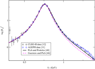
Figure 1: Comparison of the vector form factor of the pion as given by tau data and the theoretical description of Refs. [46, 48].

b) $1\,\mbox{GeV}\stackrel{{\scriptstyle<}}{{{}_{\sim}}}E\stackrel{{\scriptstyle<}}{{{}_{\sim}}}2\,\mbox{GeV}$
The extension of the description of the vector form factor of the pion at higher energies involves the inclusion of further information. Up to $2\,\mbox{GeV}$ two $\rho-$like resonances play the main role : $\rho(1450)$ and $\rho(1700)$. However the interference between resonances, the possible presence of a continuum component, etc. still deserve a study not yet done.

The inclusion of $\rho(1450)$ only improves slightly the behaviour when a Dyson-Schwinger-like resummation is performed in the framework of $R\chi T$ [53]. Lately, and based in a previous modelization proposed in Ref. [54], a procedure to extend the description of the vector form factor of the pion at higher energies has been put forward [28]. The proposal for the form factor embodies a Breit-Wigner parameterisation using the GKS model to describe $\rho(770)$, $\rho(1450)$ and $\rho(1700)$ resonances, appended with a modelization of large-$N_{C}$ QCD which sums up an infinite number of zero-width resonances to yield a Veneziano type of structure.

Figure 2: Comparison of the vector form factor of the pion in the energy region above $1\,\mbox{GeV}$ from Ref. [28]. Solid (dashed) line corresponds to the parameterisation given in Eq. (7) (Eq. (8)).

In Figure 2 it is shown how this parameterisation compares with data. The description is reasonable up to $2\,\mbox{GeV}$. Above this region there is almost no data though, in principle, it looks quite compatible with it. This model has been recently employed to analyse new Belle data [55] and it is claimed that data shows sensitivity to the $\rho(1700)$ resonance.

The key role that plays the vector form factor of the pion in the hadronic vacuum polarisation contribution to the anomalous magnetic moment of the pion [44], together with the seeming discrepancy between the predictions provided by $e^{+}e^{-}\rightarrow\pi^{+}\pi^{-}$ [50, 51] and $\tau^{-}\rightarrow\pi^{-}\pi^{0}\nu_{\tau}$ data, set up the issue of the size of isospin violation. A thorough analysis of the radiative corrections in $\tau^{-}\rightarrow\pi^{-}\pi^{0}\nu_{\tau}$ and other relevant isospin violating sources (kinematics, short-distance electroweak corrections, $\rho-\omega$ mixing) was carried out in Ref. [56]. Recently it has also been stated that further model-dependent resonance contributions not taken into account before are also relevant [57], in particular the seemingly large coupling $\rho\omega\pi$, and may correct significantly the decay rate. Additional evaluations along this claim should be done in order to reach a more sounded conclusion.

6 $\tau\rightarrow K\pi\nu_{\tau}$ : Vector and scalar form factors

The dominant contribution to the Cabibbo-suppressed tau decay rate is due to the decay $\tau\rightarrow K\pi\nu_{\tau}$. The corresponding distribution function has been measured experimentally in the past by ALEPH [58] and OPAL [59]. With the large data sets on hadronic tau decays from the B-factories both BABAR and Belle are, at present, analysing their data [20].

Assuming isospin invariance the relevant hadronic matrix element is guided by two form factors :

$$\langle\,\pi(p)\,K(p^{\prime})\,|\,\overline{s}\,\gamma_{\mu}\,u\,|\,0\,\rangle\,=\,$$

$$\left(g_{\mu\nu}-\frac{Q_{\mu}Q_{\nu}}{Q^{2}}\right)\,\left(p^{\prime}-p\right)^{\nu}\,F_{+}^{K\pi}(Q^{2})\,$$

$$+\,(p^{\prime}+p)_{\mu}\,\frac{\Delta_{K\pi}}{Q^{2}}\,F_{0}^{K\pi}(Q^{2})\,,$$ (15)

where $Q_{\mu}=(p+p^{\prime})_{\mu}$, $\Delta_{K\pi}=M_{K}^{2}-M_{\pi}^{2}$, and $F_{+}^{K\pi}$ ($F_{0}^{K\pi}$) is the vector (scalar) form factor. These have been studied within the GKS model [60]. A more thorough analysis has been carried out recently [40] where both form factors have been constructed according to the following settings :
1) Scalar form factor. We have introduced the meticulous construction given in Ref. [61], where $F_{0}^{K\pi}$ was determined from $K\pi$ scattering data by solving the corresponding dispersion relations in a coupled channel formalism.
2) Vector form factor. Following the methodology put forward in Ref. [46] we have constructed $F_{+}^{K\pi}$ by demanding it satisfies both correct chiral limit and appropriate asymptotic behaviour. We have included explicitly $K^{*}(892)$ and $K^{*}(1410)$ with a free parameter ($\gamma$) that weights the contribution of the later resonance, obtaining from the total branching ratio $\gamma=0.013\pm 0.017$ .
In Figure 3 we show the differential decay distribution of the decay and the different contributions. Notice the fundamental role played by the scalar form factor at threshold though its contribution to the branching is tiny ($\sim 10^{-4}$). Moreover we obtain $B[\tau\rightarrow K^{*}(892)\nu_{\tau}]=(1.253\pm 0.078)\%$ to be compared with the PDG value $(1.29\pm 0.05)\%$ [6].

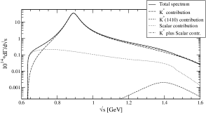
Figure 3: Differential decay distribution of the decay $\tau\rightarrow K\pi\nu_{\tau}$ and the different individual contributions computed in Ref. [40].

Between the different structure functions defined in Eq. (5) the one known as $W_{SG}$ measures the imaginary part of the interference of both form factors and requires non-trivial phases of the amplitudes that are essential for an observation of possible CP violation effects in the difference of $W_{SG}$ for the $\tau^{+}$ and $\tau^{-}$ decays :

$$W_{SG}=-2\frac{\Delta_{K\pi}}{\sqrt{Q^{2}}}\,q_{K\pi}\,\mbox{Im}\,\left[F_{+}^{K\pi}\,\left(F_{0}^{K\pi}\right)^{*}\right]\,.$$ (16)

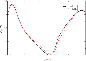
Figure 4: $W_{SG}$ structure function (normalized to $W_{tot}$) for $\tau\rightarrow K\pi\nu_{\tau}$. $\gamma=0$ corresponds to exclude the $K^{*}(1410)$ resonance.

In Figure 4 we show our result for the form factors given in Ref. [40] normalized to :

$$W_{tot}=W_{B}\,+\,\frac{3M_{\tau}^{2}}{2Q^{2}+M_{\tau}^{2}}\,W_{SA}\,\propto\,\frac{d\Gamma}{dQ^{2}}\;.$$ (17)

The experimental determination of this structure function requires, however, to measure full tau kinematics (its direction in the laboratory frame) or to handle a polarized tau.

7 $\tau^{-}\rightarrow(PPP)^{-}\nu_{\tau}$ : Vector and axial-vector form factors

The hadronic matrix element that governs the decay of the tau lepton into three pseudoscalars is parameterised by four form factors $F_{i}$ defined as :

$$\left\langle P(p_{1})P(p_{2})P(p_{3})\left|\,\left({\cal V}^{\mu}-{\cal A}^{\mu}\right)\,\right|0\right\rangle\,=$$

(18)

$$V^{\mu}_{1}F_{1}^{A}(Q^{2},s_{1},s_{2})\,+\,V^{\mu}_{2}F_{2}^{A}(Q^{2},s_{1},s_{2})$$

$$+\,Q^{\mu}\,F_{3}^{A}(Q^{2},s_{1},s_{2})\,+\,i\,V^{\mu}_{3}F_{4}^{V}(Q^{2},s_{1},s_{2})\,,$$

where

$$V^{\mu}_{1} = \left(g^{\mu\nu}-\frac{Q^{\mu}Q^{\nu}}{Q^{2}}\right)(p_{1}-p_{3})_{\nu}\,,$$

$$V^{\mu}_{2} = \left(g^{\mu\nu}-\frac{Q^{\mu}Q^{\nu}}{Q^{2}}\right)(p_{2}-p_{3})_{\nu}\,,$$

$$V^{\mu}_{3} = \varepsilon^{\mu\alpha\beta\gamma}p_{1\alpha}p_{2\beta}p_{3\gamma}\,,$$

$$Q^{\mu} = p_{1}^{\mu}+p_{2}^{\mu}+p_{3}^{\mu}\,,$$ (19)

$$s_{i} = \left(Q-p_{i}\right)^{2}\;.$$

Here $F_{i},i=1,2,3$ correspond to the axial-vector current while $F_{4}$ drives the vector current. In the particular case of three pions, we have, due to Bose-Einstein symmetry, that $F_{2}^{A}(Q^{2},s_{1},s_{2})=F_{1}^{A}(Q^{2},s_{2},s_{1})$. The scalar form factor $F_{3}^{A}$ vanishes with the mass of the Goldstone boson (chiral limit) and, accordingly, gives a tiny contribution in the three pion case. Finally the vector current only contributes, for the three-pion case, if isospin symmetry is broken as demanded by G parity conservation; hence in the isospin limit $F_{4}^{V}=0$ for this channel. It gives, in general, a non-vanishing contribution, for other final states.

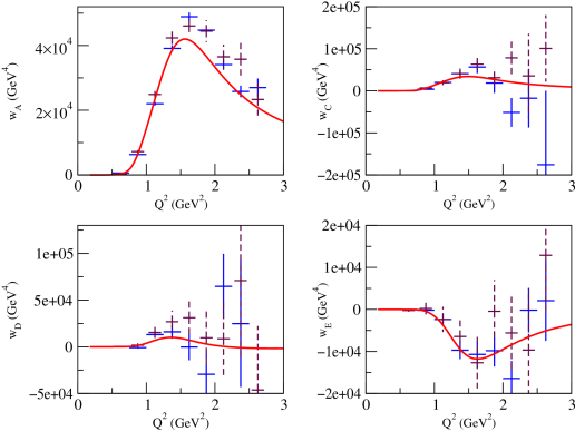
Figure 5: Theoretical predictions for the $w_{A}$, $w_{C}$, $w_{D}$ and $w_{E}$ integrated structure functions [10] for $\tau\rightarrow\pi\pi\pi\nu_{\tau}$ in comparison with the experimental data from CLEO-II (solid) [16] and OPAL (dashed) [14].

7.1 $\tau^{-}\rightarrow(\pi\pi\pi)^{-}\nu_{\tau}$

As just commented the dynamics of $\tau\rightarrow\pi\pi\pi\nu_{\tau}$ is only driven by axial-vector form factors (in the isospin limit) and, accordingly, by the presence of the axial-vector $a_{1}(1260)$ modulated by the $I=1$ vector resonances $\rho(770)(\rho)$, $\rho(1450)(\rho^{\prime})$ and $\rho(1700)(\rho^{\prime\prime})$. In the very low-energy regime the chiral constraints where explored in Ref. [62] and later it was calculated up to ${\cal O}(p^{4})$ in $\chi PT$ [42]. At higher energies resonances participate explicitly. In the GKS model the spin 1 axial-vector form factor is given by :

$$F_{1}^{A}(Q^{2},s_{i})={\cal N}|_{\chi{\cal O}(p^{2})}\,BW_{a_{1}}(Q^{2})\,\times$$

(20)

$$\times\;\frac{\displaystyle BW_{\rho}(s_{i})+\alpha\,BW_{\rho^{\prime}}(s_{i})\,+\,\beta\,BW_{\rho^{\prime\prime}}(s_{i})}{\displaystyle 1+\alpha+\beta}\;.$$

This description, complemented with an ad hoc construction of the off-shell width of the $a_{1}(1260)$ resonance, provides a good description of the spectrum of three pions [25] though a slight discrepancy shows up in the integrated structure functions [16]. The fit to the data gives the values of the $\alpha$ and $\beta$ parameters, that compute the weight of each $\rho$-like resonance and, in addition, one can study masses and on-shell widths of the participating resonances. The issue of isospin violation in this channel, within the GKS model, has also been considered [63]. Lately it was shown that this Breit-Wigner parameterisation is not consistent with chiral symmetry at ${\cal O}(p^{4})$ and thus with QCD [9, 10].

A thorough study of the axial-vector form factors in $\tau\rightarrow\pi\pi\pi\nu_{\tau}$ has been performed in Ref. [10] using the methodology described in Section 3. The authors get a parameterisation of the three pion decay of the tau lepton in terms of four free parameters : $M_{a_{1}}$, $\Gamma_{a_{1}}(M_{a_{1}})$, one combination of coupling constants of the Lagrangian and, finally, the $\alpha$ parameter in the off-shell width of the $a_{1}(1260)$ resonance in Eq. (13). Next an analysis of the ALEPH data [13] on the spectrum and branching ratio of $\tau^{-}\rightarrow\pi^{+}\pi^{-}\pi^{-}\nu_{\tau}$ is performed, obtaining $M_{a_{1}}=(1.204\pm 0.007)\,\mbox{GeV}$ and $\Gamma_{a_{1}}(M_{a_{1}}^{2})=(0.48\pm 0.02)\,\mbox{GeV}$ where the errors, given by the minimisation program, are only statistical.

OPAL [14] and CLEO [16] have collected data on the dominant structure functions in the $\tau^{-}\rightarrow\pi^{-}\pi^{0}\pi^{0}\nu_{\tau}$ decay, namely, $W_{A}$, $W_{C}$, $W_{D}$ and $W_{E}$ (5) that drive the contribution of the $J=1^{+}$ amplitude into the process and therefore the integrated structure functions over all the available phase space, defined as :

$$w_{A,C}\,=\,\int\,ds_{1}\,ds_{2}\,W_{A,C}\;,$$ (21)

$$w_{D,E}\,=\,\int\,ds_{1}\,ds_{2}\,sign\left(s_{1}-s_{2}\right)\,W_{D,E}\;.$$ (22)

CLEO [16] displays the forecast given by the GKS model and notice a slight discrepancy that shows up mainly in $w_{A}$. Then in order to have a better description they modify the model by supplying some quantum-mechanical structure (a heritage of nuclear physics that accounts for the finite size of hadrons) [64] that yields a good fit to data.

Following the results of the EFT-like Lagrangian approach explained above, and once the parameters are determined, it is possible to predict the integrated structure functions. By assuming isospin symmetry one can use the information obtained from the charged pions case to provide a description for the $\pi^{-}\pi^{0}\pi^{0}$ final hadronic state. The result and its comparison with the data is shown in Figure 5. For $w_{C}$, $w_{D}$ and $w_{E}$, it can be seen that there is a good agreement in the low $Q^{2}$ region, while for increasing energy the experimental errors become too large to state any conclusion (moreover, there seems to be a slight disagreement between both experiments at several points). On the other hand, in the case of $w_{A}$ the theoretical curve seems to lie somewhat below the data for $Q^{2}\stackrel{{\scriptstyle>}}{{{}_{\sim}}}1.5\,\mbox{GeV}^{2}$. However the study carried out in Ref. [10] seems to conclude that this is due to some inconsistency between the data by CLEO and OPAL, on one side, and ALEPH on the other.

7.2 $\tau\rightarrow(KK\pi)^{-}\nu_{\tau}$

These channels are more involved as both vector and axial-vector currents participate. Recently the CLEO Collaboration has published an analysis of the data collected on the $\tau^{-}\rightarrow K^{+}K^{-}\pi^{-}\nu_{\tau}$ decay [65]. It was known that this process is not well described by the GKS model [66] and therefore in the new analysis they have reshaped the model with two new arbitrary parameters that modulate both one of the axial-vector and the vector form factors (7). Afterward all the parameters are obtained through a reasonable fitting procedure. Along these pages we have emphasized the fact that arbitrary parameterisations are of little help in the procedure of obtaining information about non-perturbative QCD. In the CLEO example just pointed out the new parameter in the vector form factor spoils the Wess-Zumino anomaly normalisation, that appears at ${\cal O}(p^{4})$ in $\chi PT$. It is true that there are non-anomalous contributions proportional to the pseudoscalar masses at the next perturbative order that could account for a deviation but it would be surprising that the correction is around $80\%$ as the fit points out. The real issue is that, as we have indicated, the GKS model is not consistent with QCD and the CLEO reshaping is of not much use.

Previous theoretical studies of these channels have only been done within parameterisations in the line of the GKS model [27, 67]. Recently we have employed the same technique than in the three pion case to study these channels [68, 69]. The main novelty has been to handle the vector form factor through the construction of the relevant Lagrangian for the odd-intrinsic-parity sector, obtaining constraints on the new coupling constants through the requirement of the appropriate asymptotic behaviour of the vector form factor and also with some request to the phenomenology .

Our analysis emphasizes the discrepancy between different approaches in the weight of vector and axial-vector contribution to the decay width as can be seen in Table 1.

Table 1: Percentage of axial-vector and vector contribution to the total decay width in the $\tau\rightarrow KK\pi\nu_{\tau}$ channel.

Reference	Axial-vector	Vector
Our result [68]	$\sim 20\%$	$\sim 80\%$
CLEO-III [65]	$\sim 50\%$	$\sim 50\%$
[67]	$\sim 10\%$	$\sim 90\%$
[27]	$\sim 60\%$	$\sim 40\%$

8 Outlook

Hadronic decays of the tau lepton provide all-important information on the hadronization of currents in order to yield relevant knowledge on non-perturbative features of low-energy Quantum Chromodynamics. In order to achieve this goal we need to input more controlled QCD-based modelizations. Our target is not only to fit the data at whatever cost, but do it with a reasonable parameterisation that allows us to understand more about the theoretical description of Nature.

The effective theory based phenomenological Lagrangian approach seems, along this line, more promising than the Breit-Wigner parameterisations. The procedure relies in a field theory construction that embodies, up to a supposedly minor modelization of the large-$N_{C}$ behaviour, the relevant features of QCD in the resonance energy region, giving an appropriate account of the main traits of the experimental data and showing that it is a compelling framework to work with.

References

- [1] J. Portolés, Nucl. Phys. Proc. Suppl. 144 (2005) 3 [arXiv:hep-ph/0411333].
- [2] Ulf-G. Meissner, Phys. Rept. 161 (1988) 213; M. Bando, T. Kugo, K. Yamawaki, Phys. Rept. 164 (1988) 217.
- [3] S. Weinberg, Physica 96A (1979) 327.
- [4] J. Gasser and H. Leutwyler, Ann. Phys. (N.Y.) 158 (1984) 142; J. Gasser and H. Leutwyler, Nucl. Phys. B 250 (1985) 465.
- [5] H. Georgi, Ann. Rev. Nucl. Part. Sci. 43 (1993) 209; A. Pich, Proceedings of Les Houches Summer School of Theoretical Physics, (Les Houches, France, 28 July-5 September 1997), edited by R. Gupta et al. (Elsevier Science, Amsterdam 1999), Vol. II, 949, hep-ph/9806303.
- [6] W. M. Yao et al. [Particle Data Group], J. Phys. G 33 (2006) 1.
- [7] J.H. Kühn and E. Mirkes, Z. Phys. C 56 (1992) 661; J.H. Kühn and E. Mirkes, (E) idem C 67 (1995) 364.
- [8] A. Rougé, Z. Phys. C 70 (1996) 65; A. Rougé, Eur. Phys. J. C 4 (1998) 265; R.J. Sobie, Phys. Rev. D 60 (1999) 017301.
- [9] J. Portolés, Nucl. Phys. B (Proc. Suppl.) 98 (2001) 210.
- [10] D. Gómez Dumm, A. Pich and J. Portolés, Phys. Rev. D 69 (2004) 073002.
- [11] R. Barate et al, ALEPH Col., Z. Phys. C 76 (1997) 15.
- [12] S. Anderson et al , CLEO Col., Phys. Rev. D 61 (2000) 112002.
- [13] R. Barate et al, ALEPH Col., Eur. Phys. J. C 4 (1998) 409.
- [14] K. Ackerstaff, OPAL Col., Z. Phys. C 75 (1997) 593.
- [15] P. Abreu et al, DELPHI Col., Phys. Lett. B 426 (1998) 411.
- [16] T.E. Browder et al, CLEO Col., Phys. Rev. D 61 (1999) 052004.
- [17] K. Ackerstaff et al, OPAL Col., Eur. Phys. J. C 7 (1999) 571.
- [18] K.W. Edwards et al, CLEO Col., Phys. Rev. D 61 (2000) 072003.
- [19] B. Aubert et al. [BABAR Collaboration], Phys. Rev. D 72 (2005) 012003 [arXiv:hep-ex/0506007]; B. Aubert et al. [the BABAR Collaboration], Phys. Rev. D 72 (2005) 072001 [arXiv:hep-ex/0505004]; I.M. Nugent, these proceedings; R. Sobie, these proceedings; R. Kass, these proceedings.
- [20] B. Schwartz, these proceedings.
- [21] T. Ohshima, these proceedings.
- [22] M. Roney, these proceedings.
- [23] R. Decker, S. Jadach, M. Jezabek, J.H. Kühn and Z. Was, Comput. Phys. Commun. 76 (1993) 361; ibid. 70 (1992) 69; ibid. 64 (1990) 275.
- [24] H. Kühn and F. Wagner, Nucl. Phys. B 236 (1984) 16; A. Pich, Proceedings “Study of tau, charm and J/ physics development of high luminosity , Ed. L. V. Beers, SLAC (1989).
- [25] J.H. Kühn and A. Santamaría, Z. Phys. C 48 (1990) 445.
- [26] R. Decker, E. Mirkes, R. Sauer and Z. Was, Z. Phys. C 58 (1993) 445; R. Decker and E. Mirkes, Phys. Rev. D 47 (1993) 4012; R. Decker, M. Finkemeier and E. Mirkes, Phys. Rev. D 50 (1994) 6863.
- [27] M. Finkemeier and E. Mirkes, Z. Phys. C 69 (1996) 243.
- [28] C. Bruch, A. Khodjamirian and J. H. Kühn, Eur. Phys. J. C 39 (2005) 41 [arXiv:hep-ph/0409080].
- [29] G.J. Gounaris and J.J. Sakurai, Phys. Rev. Lett. 21 (1968) 244.
- [30] H. Leutwyler, Ann. of Phys. (N.Y.) 235 (1994) 165.
- [31] G. t’Hooft, Nucl. Phys. B 72 (1974) 461; E. Witten, Nucl. Phys. B 160 (1979) 57.
- [32] G. Ecker, J. Gasser, A. Pich and E. de Rafael, Nucl. Phys. B 321 (1989) 311.
- [33] G. Ecker, J. Gasser, H. Leutwyler, A. Pich and E. de Rafael, Phys. Lett. B 223 (1989) 425.
- [34] V. Cirigliano, G. Ecker, M. Eidemüller, R. Kaiser, A. Pich and J. Portolés, Nucl. Phys. B 753 (2006) 139 [arXiv:hep-ph/0603205].
- [35] M. Knecht and A. Nyffeler, Eur. Phys. J. C 21 (2001) 659; A. Pich, in Proceedings of the Phenomenology of Large QCD, edited by R. Lebed (World Scientific, Singapore, 2002), p. 239, hep-ph/0205030; G. Amorós, S. Noguera and J. Portolés, Eur. Phys. J. C 27 (2003) 243; P.D. Ruiz-Femenía, A. Pich and J. Portolés, J. High Energy Physics 07 (2003) 003; V. Cirigliano, G. Ecker, M. Eidemüller, A. Pich and J. Portolés, Phys. Lett. B 596 (2004) 96; J. Portolés and P.D. Ruiz-Femenía, Nucl. Phys. B (Proc. Suppl.) 131 (2004) 170.
- [36] I. Rosell, arXiv:hep-ph/0701248.
- [37] S.J. Brodsky and G.R. Farrar, Phys. Rev. Lett. 31 (1973) 1153; G.P. Lepage and S.J. Brodsky, Phys. Rev. D 22 (1980) 2157.
- [38] J. Bijnens, E. Gámiz, E. Lipartia and J. Prades, JHEP 0304 (2003) 055 [arXiv:hep-ph/0304222].
- [39] D. Gómez Dumm, A. Pich and J. Portolés, Phys. Rev. D 62 (2000) 054014.
- [40] M. Jamin, A. Pich and J. Portolés, Phys. Lett. B 640 (2006) 176 [arXiv:hep-ph/0605096].
- [41] J. Gasser and H. Leutwyler, Nucl. Phys. B 250 (1985) 517; J. Bijnens, G. Colangelo and P. Talavera, J. High Energy Phys. 05 (1998) 014; J. Bijnens and P. Talavera, J. High Energy Phys. 03 (2002) 046.
- [42] G. Colangelo, M. Finkemeier and R. Urech, Phys. Rev. D 54 (1996) 4403.
- [43] G. Colangelo, M. Finkemeier, E. Mirkes and R. Urech, Nucl. Phys. B (Proc. Suppl.) 55C (1997) 325.
- [44] M. Davier, these proceedings.
- [45] J.F. de Trocóniz and F.J. Ynduráin, Phys. Rev. D 65 (2002) 093001.
- [46] F. Guerrero and A. Pich, Phys. Lett. B 412 (1997) 382.
- [47] J.A. Oller, E. Oset and J.E. Palomar, Phys. Rev. D 63 (2001) 114009.
- [48] A. Pich and J. Portolés, Phys. Rev. D 63 (2001) 093005.
- [49] A. Pich and J. Portolés, Nucl. Phys. B (Proc. Suppl.) 121 (2003) 179.
- [50] R. R. Akhmetshin [CMD-2 Collaboration], arXiv:hep-ex/0610021.
- [51] A. Aloisio et al. [KLOE Collaboration], Phys. Lett. B 606 (2005) 12 [arXiv:hep-ex/0407048].
- [52] G. Pancheri, O. Shekhovtsova and G. Venanzoni, Phys. Lett. B 642 (2006) 342 [arXiv:hep-ph/0605244].
- [53] J.J. Sanz-Cillero and A. Pich, Eur. Phys. J. C 27 (2003) 587.
- [54] C.A. Domínguez, Phys. Lett. B 512 (2001) 331.
- [55] K. Abe et al. [Belle Collaboration], arXiv:hep-ex/0512071; M. Fujikawa, these proceedings.
- [56] V. Cirigliano, G. Ecker and H. Neufeld, J. High Energy Phys. 08 (2002) 002.
- [57] F. Flores-Baez, A. Flores-Tlalpa, G. López Castro and G. Toledo Sánchez, Phys. Rev. D 74 (2006) 071301 [arXiv:hep-ph/0608084]; G. López Castro, these proceedings.
- [58] R. Barate et al. [ALEPH Collaboration], Eur. Phys. J. C 11 (1999) 599 [arXiv:hep-ex/9903015].
- [59] G. Abbiendi et al. [OPAL Collaboration], Eur. Phys. J. C 35 (2004) 437 [arXiv:hep-ex/0406007].
- [60] M. Finkemeier and E. Mirkes, Z. Phys. C 72 (1996) 619 [arXiv:hep-ph/9601275].
- [61] M. Jamin, J. A. Oller and A. Pich, Nucl. Phys. B 622 (2002) 279 [arXiv:hep-ph/0110193].
- [62] R. Fischer, J. Wess and F. Wagner, Z. Phys. 3 (1980) 313.
- [63] E. Mirkes and R. Urech, Eur. Phys. J. C 1 (1998) 201.
- [64] D.M. Asner et al, CLEO Col., Phys. Rev. D 61 (2000) 012002.
- [65] T.E. Coan et al, CLEO Col., Phys. Rev. Lett. 92 (2004) 232001.
- [66] F. Liu, Nucl. Phys. B (Proc. Suppl.) 123 (2003) 66.
- [67] J. J. Gómez- Cadenas, M. C. González- García and A. Pich, Phys. Rev. D 42 (1990) 3093.
- [68] P. Roig, “Hadronic decays of the lepton: channels”, Master Thesis, Universitat de València (2006).
- [69] D. Gómez Dumm, P. Roig, A. Pich and J. Portolés, work in preparation.