Heat conductivity of a pion gas

Abstract

We evaluate the heat conductivity of a dilute pion gas employing the Uehling-Uehlenbeck equation and experimental phase-shifts parameterized by means of the $SU(2)$ Inverse Amplitude Method. Our results are consistent with previous evaluations. For comparison we also give results for an (unphysical) hard sphere gas.

1 Transport coefficients

Transport coefficients in heavy-ion collisions remain of interest as prospects for direct experimental measurement at RHIC improve. In particular, elliptic flow has been proposed Teaney:2003kp as a tell-tale for viscous effects. There have also recently been a number of papers emphasizing viscosity (for example Liu:2006cs , Nakano:2006wy ) following recent insight from conformal field theory Policastro:2001yc . Follow-up studies are under preparation by several groups from the hadron and from the quark-gluon phases in RHIC-theory to see the effect of the phase transition on the viscosity.

Although we have presented a comprehensive study of the shear viscosity of a hadronic gas at low temperature Dobado:2003wr , in this brief report we focuse on another transport coefficient, the thermal conductivity, associated to energy conservation and flow in the hot gas.

We employ the same notation and conventions as in our earlier publication Dobado:2003wr . In particular we employ the $SU(2)$ Inverse Amplitude Method parametrization of the pion-pion scattering experimental phase shifts (as well as alternative parametrizations to check the sensitivity of the calculation presented). Note we also employ the Landau convention for the flows as opposed to the Eckart convention that has also been widely used Gavin:1985ph .

To make this paper minimally self-contained, we collect here a few of the key results and assumptions.

We are working in a pion gas at temperatures well below any phase transition, in the dilute approximation near equilibrium. The equilibrium equation of state yields an enthalpy per unit volume $h=P+\rho$ as

$$h=\frac{g_{\pi}m_{\pi}^{4}}{4\pi^{2}}\int_{0}^{\infty}dx\frac{\sqrt{x}(1+4x/3)}{\sqrt{x+1}\left(z^{-1}e^{y(\sqrt{1+x}-1)}-1\right)}$$ (1)

and the particle (pion) density is given by

$$n\left(y=\frac{m_{\pi}}{T},z\right)=\frac{g_{\pi}m_{\pi}^{3}}{4\pi^{2}}\int_{0}^{\infty}dx\frac{x^{1/2}}{z^{-1}e^{y(\sqrt{1+x}-1)}-1}$$ (2)

($z=e^{(\mu-m)/T}$ being the fugacity).

We take a constant perturbation around equilibrium proportional to the relativistic temperature-pressure gradient

$$\delta f({\bf p})=\frac{f_{0}}{T}\frac{{\bf p}}{\arrowvert{\bf p}\arrowvert}g(\arrowvert{\bf p}\arrowvert)\left[{\bf\nabla}T-\frac{T}{h}{\bf\nabla}P\right]$$ (3)

and change the variable to $x=(p/m_{\pi})^{2}$. We perform a polynomial expansion of $g(x)$, and display results for the first order only, $g(x)=A_{0}$, with $A_{0}$ a constant. Convergence is known to be fast. Since pions are not exactly massless, no singularities appear that might require a more careful treatment Manuel:2004iv and the only reason to improve on this variational calculation would be to improve its accuracy beyond the 10% level. This program has been carried out at least for the non-relativistic pion gas viscosity in ref. Dobado:2001jf . We have also made minimum sensitivity checks based on a simple numeric Gram-Schmidt polynomial construction beyond $A_{0}$ but will report them elsewhere.

From the standard linearized (Boltzmann) Uehling-Uehlenbeck transport equation one can derive the following for this perturbation near equilibrium:

$$A_{0}=\frac{I_{1}(y,z)}{I_{2}(y,z)}$$ (4)

$$I_{1}=2\pi m_{\pi}^{3}y\int_{0}^{\infty}\frac{xdx}{\sqrt{1+x}}f(E(x))\left(\sqrt{1+x}-\frac{h}{m_{\pi}n}\right)$$ (5)

$$I_{2}=\frac{1}{4A^{2}}\int[d\Phi]\left[e^{\beta(\omega-2\mu)}ff^{\prime}f_{1}f^{\prime}_{1}\right.$$ (6)

$$\left.\Delta_{i}\left({\bf\hat{p}_{i}}\left[1-e^{-\beta(E_{i}-\mu)}\right]\right)\cdot\Delta_{j}\left({\bf\hat{p}_{j}}\left[1-e^{-\beta(E_{j}-\mu)}\right]\right)\right]$$

where $\omega$ denotes the total energy ($\omega=E+E_{1}=E^{\prime}+E^{\prime}_{1}$) , $A$ is the inverse normalization constant of the distribution functions

$$A=\xi_{\pi}^{-1}=\frac{g_{\pi}}{(2\pi)^{3}}$$

($g_{\pi}=3$ for isospin degeneracy) and the last term is a shorthand for the symmetrization

$$\Delta_{i}\left({\bf\hat{p}_{i}}\left[1-e^{-\beta(E_{i}-\mu)}\right]\right)=$$ (7)

$$\left({\bf\hat{p}^{\prime}_{1}}\left[1-e^{-\beta(E^{\prime}_{1}-\mu)}\right]+{\bf\hat{p}^{\prime}}\left[1-e^{-\beta(E^{\prime}-\mu)}\right]-\right.$$

$$\left.{\bf\hat{p}_{1}}\left[1-e^{-\beta(E_{1}-\mu)}\right]-{\bf\hat{p}}\left[1-e^{-\beta(E-\mu)}\right]\right)\ .$$

Once $A_{0}$ has been thus computed, the heat conductivity follows as

$$\kappa=-\frac{hm_{\pi}^{3}2\pi A}{3nT}A_{0}l_{1}(y,z)$$ (8)

with

$$l_{1}(y,z)=\int_{0}^{\infty}\frac{xdx}{\sqrt{1+x}\left(z^{-1}e^{y(\sqrt{1+x}-1)}-1\right)}$$ (9)

To evaluate the integral in $I_{2}$ in Eq. (4) we employ a Montecarlo computer program. Without loss of generality we can choose the total momentum directed along the $OZ$ axis. The independent variables can be taken as $P$ and $\omega$ (respectively the total momentum and energy in a binary collision), $p=\arrowvert{\bf p}\arrowvert$ and $p^{\prime}=\arrowvert{\bf p}^{\prime}\arrowvert$ (the incoming and outgoing pion momenta for one of the two pions, the other being fixed by momentum conservation). Finally the outgoing pion with momentum $p^{\prime}$ does not need to be in the same plane as ${\bf P}$ and ${\bf p}$, and therefore we need an azimuthal angle $\phi^{\prime}$ for this momentum. The cosines of the polar angles associated to ${\bf p}$ and $\bf{p^{\prime}}$ are fixed by the energy conservation relation

$$\delta\left(\omega-E-E_{1}\right)=\frac{E_{1}}{pP}\,\delta(x-x_{0})$$

and the associated integrals are immediately performed, with

$$x_{0}=\frac{P^{2}+\omega(2E-\omega)}{2pP}$$ (10)

$$x_{0}^{\prime}=\frac{P^{2}+\omega(2E^{\prime}-\omega)}{2p^{\prime}P}\ .$$ (11)

In addition, rigid rotations around ${\bf P}$ parametrized by $\phi$ are trivial and lead to a factor of $2\pi$, and global rotations of the system (the angles associated to ${\bf P}$) are also trivial and yield another $4\pi$.

Putting all together, the phase space integration
weighted with the square scattering amplitude can be expressed as

$$\int[d\Phi]=\int v_{rel}d\sigma d{\bf p}d{\bf p}^{\prime}=$$ (12)

$$\int dPdpdp^{\prime}d\omega d\phi^{\prime}\arrowvert T\arrowvert^{2}\frac{4\pi 2\pi}{4\pi^{2}}\frac{1}{4EE_{1}}\frac{p^{\prime}}{E^{\prime}_{1}}\frac{p^{\prime}}{E^{\prime}}\frac{E_{1}}{pP}\frac{E_{1}^{\prime}}{p^{\prime}P}P^{2}p^{2}\$$

Our numerical results for the thermal conductivity are displayed in the figures.

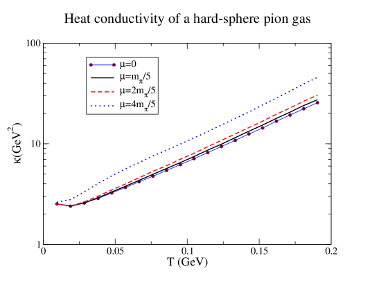
Figure 1: We show the $\mu$ dependence of the conductivity for the hard-sphere gas appoximation

In Fig. 1 we plot the heat conductivity as a function of temperature, at several $\mu$’s in the hard-sphere scattering case, that is, when we use a constant scattering amplitude based on Weinberg’s low energy theorem:

$$\left|T\right|^{2}=\frac{23}{3}\frac{m_{\pi}^{4}}{f_{\pi}^{4}}$$ (13)

For no $\mu$ does the heat conductivity diverge at low temperature to the reach of our Montecarlo. In the high temperature limit we expect on dimensional grounds, and numerically find, $\kappa=A\cdot T^{2}$, where the numerical constant is close to $A=685$.

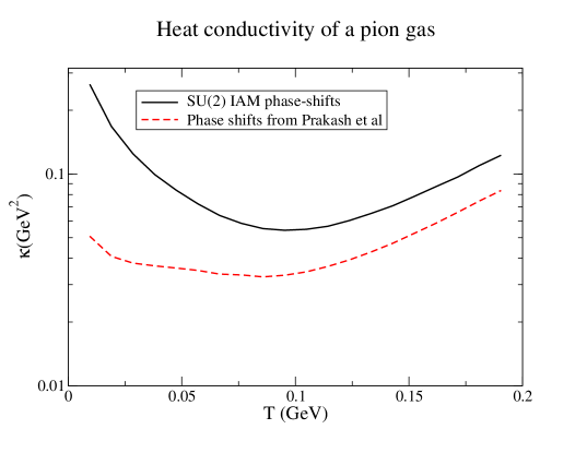
Figure 2: Thermal conductivity $\kappa$ from SU(2) chiral perturbation theory unitarized by means of the Inverse Amplitude Method. The pion chemical potential is taken to be $\mu_{\pi}=0$.

In Fig. 2, employing IAM phase shifts, that unitarize a higher order $O(p^{4})$ in chiral perturbation theory Dobado:1989qm , and therefore introduce a dependence with the energy for the pion-pion scattering amplitude, we now find that there is a minimum value near $T_{c}=100$ MeV and $\kappa\to\infty$ when $T\to 0$. The high $T$ scaling is close to the dimensional analysis even at the moderately large plotted temperatures,

$$\kappa\propto 3.4\,T^{2}\ .$$

In the figure we also show our own Montecarlo-based calculation of the heat conductivity employing the simple resonance saturation parametrization for the isoscalar and isovector phase shifts by the Brookhaven group Prakash:1993bt , for comparison and to give an idea of the sensitivity to the parametrization.

Next in Fig. 3 we show the comparison with the existing computation of D. Davesne Davesne:1995ms of both calculations

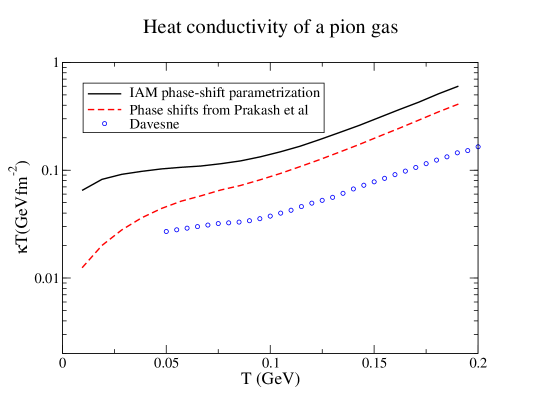
Figure 3: Thermal conductivity times temperature $T\kappa$ from SU(2) chiral perturbation theory unitarized by means of the Inverse Amplitude Method. The pion chemical potential is taken to be $\mu_{\pi}=0$. We also plot the computation with the phase-shifts of Prakash:1993bt and compare them to D. Davesne’s evaluation.

Note also a recent calculation by Muroya:2004pu that employs chiral perturbation theory alone (without unitarization). This approach features an ever-increasing cross section, unphysical behavior that artificially shortens the mean free path and therefore lowers the transport coefficients. Therefore the validity of the results is limited to low temperatures. However a direct comparison with this approach is difficult since the authors directly include the effect of baryon resonances.

In conclusion, from published calculations and our own contribution we see that we have a fair theoretical idea on how the thermal conductivity of a pure pion gas should behave with temperature. We have further studied its behavior with chemical potential that is important because chemical freeze-out is expected to occur before thermal freeze out in Heavy-Ion Collisions, the reason being that the low energy hadron interactions are elastic scattering, largely mediated by resonances (automatically incorporated in our Inverse Amplitude Method Phase shifts).

This work has been supported by research grants FPA 2004-02602, 2005-02327, PR27/05-13955-BSCH and has been presented at the IVth International Conference on Quarks and Nuclear Physics, Madrid, Spain, June 5th-10th 2006. We thank A. Gómez Nicola and D. Fernández-Fraile for informing us that their own calculation along the lines of Fernandez-Fraile:2006sk in chiral perturbation theory also yields analogous results.

References

- (1) D. Teaney, Phys. Rev. C 68 (2003) 034913 [arXiv:nucl-th/0301099].
- (2) H. Liu, D. Hou and J. Li, arXiv:hep-ph/0609034.
- (3) E. Nakano, arXiv:hep-ph/0612255.
- (4) G. Policastro, D. T. Son and A. O. Starinets, Phys. Rev. Lett. 87 (2001) 081601 [arXiv:hep-th/0104066].
- (5) A. Dobado and F. J. Llanes-Estrada, Phys. Rev. D 69 (2004) 116004 [arXiv:hep-ph/0309324].
-
(6)
S. Gavin,
Nucl. Phys. A 435 (1985) 826;
W. A. van Leeuwen and S. R. de Groot, Physica 51 (1971) 1. - (7) C. Manuel, A. Dobado and F. J. Llanes-Estrada, JHEP 0509 (2005) 076 [arXiv:hep-ph/0406058].
- (8) A. Dobado and S. N. Santalla, Phys. Rev. D 65 (2002) 096011 [arXiv:hep-ph/0112299].
- (9) A. Dobado, M. J. Herrero and T. N. Truong, Phys. Lett. B 235 (1990) 134.
- (10) M. Prakash, M. Prakash, R. Venugopalan and G. Welke, Phys. Rept. 227 (1993) 321.
- (11) D. Davesne, Phys. Rev. C 53 (1996) 3069.
- (12) S. Muroya and N. Sasaki, Prog. Theor. Phys. 113 (2005) 457 [arXiv:nucl-th/0408055].
- (13) D. Fernandez-Fraile and A. Gómez-Nicola, arXiv:hep-ph/0610197.