Weakly-bound Hadronic Molecule
near a 3-body Threshold

Abstract

The $X(3872)$ seems to be a loosely-bound hadronic molecule whose constituents are two charm mesons. A novel feature of this molecule is that the mass difference of the constituents is close to the mass of a lighter meson that can be exchanged between them, namely the pion. We analyze this feature in a simple model with spin-0 mesons only. Various observables are calculated to next-to-leading order in the interaction strength of the exchanged meson. Renormalization requires summing a geometric series of next-to-leading order corrections. The dependence of observables on the ultraviolet cutoff can be removed by renormalizations of the mass of the heaviest meson, the coupling constant for the contact interaction between the heavy mesons, and short-distance coefficients in the operator product expansion. The next-to-leading order correction has an unphysical infrared divergence at the threshold of the two heavier mesons that can be eliminated by a further resummation that takes into account the nonzero width of the heaviest meson.

I Introduction

The $X(3872)$ is a new hadronic resonance discovered in 2003 by the Belle Collaboration Choi:2003ue and subsequently confirmed by the CDF, Babar, and D0 Collaborations Acosta:2003zx ; Abazov:2004kp ; Aubert:2004ns . All the properties of the $X(3872)$ that have been measured thus far are compatible with its identification as a weakly-bound molecule whose constituents are a superposition of the charm meson pairs $D^{*0}\bar{D}^{0}$ and $D^{0}\bar{D}^{*0}$ Tornqvist:2003na ; Close:2003sg ; Pakvasa:2003ea ; Voloshin:2003nt ; Wong:2003xk ; Braaten:2003he ; Swanson:2003tb ; Braaten:2004rw ; Tornqvist:2004qy ; Braaten:2004fk ; Swanson:2004pp ; Voloshin:2004mh ; Braaten:2004ai ; Braaten:2005jj ; AlFiky:2005jd ; Braaten:2005ai ; Suzuki:2005ha ; Swanson:2006st ; Braaten:2006sy ; AbdEl-Hady:2006ds ; Colangelo:2007ph .

Because it is so weakly bound, the $X(3872)$ has many features in common with the deuteron, which is a weakly-bound baryonic molecule consisting of a proton and a neutron. Their binding energies are both small compared to the natural energy scale associated with pion exchange: $m_{\pi}^{2}/(2M_{12})$, where $M_{12}$ is the reduced mass of the two constituents. The binding energy 2.2 MeV of the deuteron is small compared to the natural scale of about 20 MeV. After taking into account a recent precision measurement of the $D^{0}$ mass by the CLEO Collaboration Cawlfield:2007dw , the difference between the measured mass of the $X(3872)$ and the $D^{*0}\bar{D}^{0}$ threshold is

$$M_{X}-(M_{1}+M_{2})=-0.6\pm 0.6\ {\rm MeV}.$$ (1)

This is small compared to the natural energy scale of about 10 MeV. The Belle Collaboration has set an upper bound on the width of the $X$ Choi:2003ue :

$$\Gamma_{X}<2.3\ {\rm MeV}\hskip 28.45274pt(90\%\ {\rm C.L.}).$$ (2)

This is also small compared to the natural energy scale. The small width is most easily understood if the $X$ is below the $D^{*0}\bar{D}^{0}$ threshold.

Because the binding energies of the deuteron and the $X(3872)$ are small compared to the natural energy scales, they have universal properties that are determined by the large scattering length $a$ of the constituents Braaten:2003he . The universality of few-body systems with a large scattering length has many applications in atomic, nuclear, and particle physics Braaten:2004rn . The universal features of the $X(3872)$ were first exploited by Voloshin to describe its decays into $D^{0}\bar{D}^{0}\pi^{0}$ and $D^{0}\bar{D}^{0}\gamma$, which can proceed through decay of the constituent $D^{*0}$ or $\bar{D}^{*0}$ Voloshin:2003nt . Universality has also been applied to the production process $B\to KX$ Braaten:2004fk ; Braaten:2004ai , to the line shape of the $X$ Braaten:2005jj , and to decays of $X$ into $J/\psi$ and pions Braaten:2005ai . These applications rely on factorization formulas that separate the length scale $a$ from all the shorter distance scales of QCD Braaten:2005jj . The factorization formulas can be derived using the operator product expansion for a low-energy effective field theory Braaten:2006sy .

There is one feature of the $X(3872)$ that is very different from the deuteron. The mass difference between the constituents $D^{*0}$ and $\bar{D}^{0}$, $M_{2}-M_{1}=142.12\pm 0.07$ MeV, is very close to the $\pi^{0}$ mass: $m=134.98$ MeV. Thus the $D^{*0}$ mass is very close to the $D^{0}\pi^{0}$ threshold: $M_{2}-M_{1}-m=7.14\pm 0.07$ MeV. This is important because the pion is the lightest meson that can be exchanged between the $D^{*0}$ and $\bar{D}^{0}$. The small energy gap between the $D^{*0}$ mass and the $D^{0}\pi^{0}$ threshold makes it easy for the $D^{*0}$ to make a transition to $D^{0}\pi^{0}$. An important consequence is that the $X$ could have a substantial 3-body component $D^{0}\bar{D}^{0}\pi^{0}$. Suzuki has argued that the near equality of $M_{2}-M_{1}$ and $m$ implies that the pion-exchange interaction is too weak to bind the $X$ Suzuki:2005ha , but this conclusion has been criticized Swanson:2006st .

An analysis of the effect of the near equality $M_{2}-M_{1}\approx m$ in the case of the $X(3872)$ is complicated by other effects that may be comparable in importance. There are other nearby two-body and three-body thresholds. The thresholds for the charged mesons $D^{*+}D^{-}$ and $D^{+}D^{*-}$ are higher than the $D^{*0}\bar{D}^{0}$ threshold by $8.08\pm 0.12$ MeV. The $D^{0}D^{-}\pi^{+}$ and $D^{+}\bar{D}^{0}\pi^{-}$ thresholds are higher than the $D^{*0}\bar{D}^{0}$ threshold by only $2.23\pm 0.12$ MeV. There are several other features that complicate the analysis of the effects of pions on the $X$. The constituent $D^{*}$’s are spin-1 particles. The charge conjugation $C=+$ requires the molecule to be a superposition of charm mesons: $D^{*0}\bar{D}^{0}+D^{0}\bar{D}^{*0}$. The interaction of the charm mesons with pions depends on the pion momentum. A quantitative analysis of the effects of pions on the $X$ might require all these effects to be taken into account.

Since the new feature of the $X(3872)$ is the near equality between the mass difference $M_{2}-M_{1}$ of the constituents and the mass $m$ of a meson that can be exchanged between them, it is worthwhile to analyze this feature in a simple model that avoids all the other complications of the $X$. The simplest such model is one in which the primary constituents $D_{1}$ and $D_{2}$ are spin-0 mesons with a large positive scattering length and a momentum-independent coupling to a lighter spin-0 meson $\phi$. We will calculate the effects of the exchanged meson in this model to next-to-leading order in the $D_{2}-D_{1}\phi$ coupling constant $g$.

In Sec. II, we write down the lagrangian for the model and discuss its parameters. In Sec. III, we summarize the results of the model at 0^th order in $g$ that were derived previously in Refs. Braaten:2005jj ; Braaten:2006sy . The results include the short-distance production rate for $X$ and the line shape of $X$ in a short-distance decay channel. The ultraviolet divergences can be removed by renormalization of the coupling constant for the $D_{1}D_{2}$ contact interaction and by renormalization of short-distance coefficients in the operator product expansion. In Sec. IV, we calculate the observables in Sec. III to next-to-leading order in $g$. We also calculate the short-distance production rate for $D_{1}D_{1}\phi$ and the decay rate of $X$ into $D_{1}D_{1}\phi$. There are new ultraviolet divergences that can be removed by renormalization of the $D_{2}$ mass. We show that after summing a geometric series of next-to-leading order corrections, all remaining ultraviolet divergences can again be removed by renormalization of the coupling constant for the $D_{1}D_{2}$ contact interaction and by renormalization of short-distance coefficients in the operator product expansion. A further resummation is required to eliminate an infrared divergence at the $D_{1}D_{2}$ threshold in the next-to-leading order corrections. In Sec. V, we summarize our results. The two-loop Feynman diagrams that arise at next-to-leading order in $g$ are calculated in an Appendix.

II A Scalar Meson Model

II.1 Lagrangian

We consider the simplest possible model with a bound state $X$ whose mass is close to a 3-body threshold. The primary constituents $D_{1}$ and $D_{2}$ of the bound state are scalar mesons whose masses $M_{1}$ and $M_{2}$ satisfy $M_{1}<M_{2}$. There is also a scalar meson $\phi$ whose mass $m$ is close to the mass difference $M_{2}-M_{1}$. We will refer to this model as the scalar meson model. It is defined by a nonrelativistic quantum field theory with three complex scalar fields $D_{1}$, $D_{2}$, and $\phi$. The free terms in the lagrangian are

$${\cal L}_{\rm free}=\sum_{i=1,\,2}D_{i}^{\dagger}\left(i\frac{\partial}{\partial t}-M_{i}+\frac{1}{2M_{i}}\nabla^{2}\right)D_{i}+\phi^{\dagger}\left(i\frac{\partial}{\partial t}-m+\frac{1}{2m}\nabla^{2}\right)\phi.$$ (3)

The interaction terms for the scalar meson model are

$${\cal L}_{\rm int}=-\lambda_{0}D_{1}^{\dagger}D_{2}^{\dagger}D_{1}D_{2}-g\big{(}D_{2}^{\dagger}D_{1}\phi+D_{1}^{\dagger}\phi^{\dagger}D_{2}\big{)}-\delta MD_{2}^{\dagger}D_{2}.$$ (4)

The interaction vertices are illustrated in Fig. 1. The coupling constants $\lambda_{0}$ and $g$ have mass dimensions $-2$ and $-1/2$, respectively. We assume that there is a fine-tuning that makes the $D_{1}D_{2}$ scattering length large, which implies that the $D_{1}D_{2}$ contact interaction with coupling constant $\lambda_{0}$ must be treated nonperturbatively. The subscript on $\lambda_{0}$ emphasizes that it is a bare coupling constant that requires renormalization. We assume that the $D_{2}-D_{1}\phi$ interaction can be treated perturbatively and we calculate its effects through order $g^{2}$. At this order, no renormalization of $g$ is required. However, we will see that nonperturbative renormalization of $\lambda_{0}$ requires summing a geometric series to all orders in $g^{2}$. There are also ultraviolet divergent corrections to the mass of the $D_{2}$ which are cancelled by the mass counterterm $\delta M$ in Eq. (4).

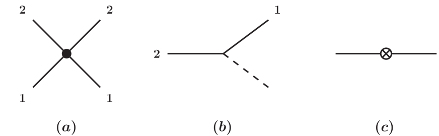
Figure 1: Vertices for (a) the $D_{1}D_{2}$ contact interaction, (b) the $D_{1}D_{2}\phi$ interaction, and (c) the $D_{2}$ mass counterterm.

II.2 Masses

It is convenient to introduce concise notations for various combinations of the masses. The sum and difference of the $D_{1}$ and $D_{2}$ masses are

$$M_{1+2} = M_{1}+M_{2},$$ (5a)

$$M_{2-1} = M_{2}-M_{1}.$$ (5b)

The reduced masses of $D_{1}D_{2}$ and of $D_{1}\phi$ are

$$M_{12} = \frac{M_{1}M_{2}}{M_{1}+M_{2}},$$ (6a)

$$m_{1} = \frac{M_{1}m}{M_{1}+m}.$$ (6b)

If $m$ is much smaller than $M_{1}$, the natural energy and 3-momentum scales associated with exchange of the meson $\phi$ between the mesons $D_{1}$ and $D_{2}$ are $m^{2}/M_{12}$ and $m$, respectively. We assume that the energy gap between the $D_{2}$ mass and the $D_{1}\phi$ threshold is small compared to the natural energy scale:

$$M_{2-1}-m\ll m^{2}/M_{12}.$$ (7)

The total number of heavy mesons $D_{1}$ and $D_{2}$ is conserved by the interactions in Eq. (4). We are interested in the sector of the theory with two heavy mesons and, more specifically, in the threshold region where the invariant mass $M$ of all the particles is very close to $M_{1+2}$:

$$|M-M_{1+2}|\ll m^{2}/M_{12}.$$ (8)

This restricts the possible scattering states to $D_{1}D_{2}$ and $D_{1}D_{1}\phi$.

For numerical illustrations, we will use masses that correspond to the $D^{*0}\bar{D}^{0}/D^{0}\bar{D}^{0}\pi^{0}$ system. The meson masses are $M_{2}=2006.7$ MeV, $M_{1}=1864.5$ MeV, and $m=135.0$ MeV. Thus $M_{12}\approx 966$ MeV and $M_{2-1}-m=7.2$ MeV. The natural energy scale is $m^{2}/M_{12}\approx 19$ MeV. The condition in Eq. (7) is only marginally satisfied: $M_{12}(M_{2-1}-m)/m^{2}\approx 0.4$. We take the binding energy of $X$ to be $E_{X}=0.4$ MeV, which is near the central value of the measurement of $M_{X}$ in Eq. (1). If we express this binding energy as $E_{X}=\kappa_{X}^{2}/(2M_{12})$, the binding momentum is $\kappa_{X}=27.8$ MeV.

II.3 Coupling constants

We impose an ultraviolet cutoff on the momenta $\vec{p}\,$ of particles in the center-of-momentum frame that restricts them to the region $|\vec{p}\,|\ll m$. This guarantees that all the particles remain nonrelativistic. It was shown in Ref. Braaten:2006sy that at leading order $g^{0}$, all ultraviolet divergences can be absorbed into $\lambda_{0}$ and into short-distance coefficients in the operator product expansion. At order $g^{2}$, there are new ultraviolet divergences that can be absorbed into the $D_{2}$ mass. We will find that the remaining ultraviolet divergences can again be absorbed into $\lambda_{0}$ and into short-distance coefficients in the operator product expansion.

The coupling constant $\lambda_{0}$ must be tuned to near the critical value at which the $D_{1}D_{2}$ scattering length diverges in order for the bound state $X$ to have a small binding energy $E_{X}\ll m^{2}/M_{12}$. In order to compare results at order $g^{0}$ and order $g^{2}$, we must have a well-defined renormalization prescription for $\lambda_{0}$ or, equivalently, a clear definition of the binding energy $E_{X}$. We will find that all the amplitudes for processes near the $D_{1}D_{2}$ threshold have a resonant term with a common factor $\mathcal{A}(E)$ that depends on the energy $E$ in the rest frame. For example, the line shape in a short-distance decay channel of $X$ produced by a short-distance process has a long-distance factor $|\mathcal{A}(M)|^{2}$, where $M$ is the invariant mass of the decay products. The square of the resonant factor can be expressed in the form

$$|\mathcal{A}(E)|^{2}=\frac{1}{[{\rm Re}\,\mathcal{A}^{-1}(E)]^{2}+[{\rm Im}\,\mathcal{A}^{-1}(E)]^{2}}.$$ (9)

As a function of the real energy $E$, this resonance factor has a peak when $E$ is close to $M_{1+2}-E_{X}$. The peak arises because ${\rm Re}\,\mathcal{A}^{-1}(E)$ vanishes near that value of $E$ and ${\rm Im}\,\mathcal{A}^{-1}(E)$ is much smaller than ${\rm Re}\,\mathcal{A}^{-1}(E)$ except near that value of $E$. As our renormalization prescription for $\lambda_{0}$, we demand that ${\rm Re}\,\mathcal{A}^{-1}(E)$ vanishes at an energy determined by a real variable $\kappa_{X}$:

$${\rm Re}\,\mathcal{A}^{-1}(E)=0\hskip 28.45274pt{\rm at\ }E=M_{1+2}-\kappa^{2}_{X}/(2M_{12}).$$ (10)

The dependence of an observable on the bare parameter $\lambda_{0}$ can be eliminated in favor of the renormalization parameter $\kappa_{X}$. We assume that $\kappa_{X}$ is small compared to the natural momentum scale: $\kappa_{X}\ll m$.

The amplitude $\mathcal{A}(E)$ has a pole at a complex energy $E_{\rm pole}$ near the real energy at which $|\mathcal{A}(E)|^{2}$ has its maximum. We choose to define the mass $M_{X}$ and the width $\Gamma_{X}$ of $X$ by expressing that complex energy in the form

$$E_{\rm pole}\equiv M_{X}-i\Gamma_{X}/2.$$ (11)

We also choose to define the binding energy $E_{X}$ by

$$E_{X}\equiv M_{1+2}-M_{X}.$$ (12)

We assume that the binding energy and the width of $X$ are both small compared to the natural energy scale: $E_{X},\Gamma_{X}\ll m^{2}/M_{12}$.

In Ref. Braaten:2006sy , the authors proposed a renormalization scheme in which $\lambda_{0}$ was tuned to give a prescribed value for the complex parameter $E_{\rm pole}$. The binding energy $E_{X}$ and the width $\Gamma_{X}$ were taken as the input parameters that determine $E_{\rm pole}$. This renormalization scheme requires $\lambda_{0}$ to be a complex coupling constant. The imaginary part of $\lambda_{0}$ takes into account inelastic scattering channels for $D_{1}D_{2}$ that are outside the energy range described by the effective field theory. In this paper, we assume that any such inelastic channels do not give a significant contribution to the width of $X$. The coupling constant $\lambda_{0}$ is therefore real valued. We could use the binding energy $E_{X}$ as the input parameter and eliminate $\lambda_{0}$ in favor of $E_{X}$, and then $\Gamma_{X}$ would be calculable. We find it more convenient to eliminate $\lambda_{0}$ in favor of the variable $\kappa_{X}$ introduced in Eq. (10). In this renormalization scheme, $E_{X}$ and $\Gamma_{X}$ are both calculable in terms of $\kappa_{X}$, $g$, and the masses $M_{1}$, $M_{2}$, and $m$.

The most convenient input for determining the coupling constant $g$ is the width $\Gamma_{2}$ of the heavy meson $D_{2}$. Since $M_{2}>M_{1}+m$, the $D_{1}D_{2}\phi$ vertex in Fig. 1(b) allows $D_{2}$ to decay into $D_{1}\phi$. Calculating the width using nonrelativistic phase space, we obtain

$$\Gamma_{2}=\frac{g^{2}m_{1}}{\pi}\left[2m_{1}(M_{2-1}-m)\right]^{1/2},$$ (13)

where $M_{12}$ and $m_{1}$ are the reduced masses defined in Eqs. (6). The value of the coupling constant $g$ can be determined from $\Gamma_{2}$ and the masses. We assume that the width of $D_{2}$ is small compared to the natural energy scale: $\Gamma_{2}\ll m^{2}/M_{12}$. We also assume $\Gamma_{2}$ is small enough to allow perturbation theory in the coupling constant $g$.

For numerical illustrations, we will use values of the parameters that correspond to the $D^{*0}\bar{D}^{0}/D^{0}\bar{D}^{0}\pi^{0}$ system. We take the width of $D_{2}$ to be $\Gamma_{2}=0.07$ MeV, which is approximately the total width for $D^{*0}$ Braaten:2005jj . This is much smaller than the natural energy scale $m^{2}/M_{12}$ and also rather small compared to $M_{2-1}-m$: $\Gamma_{2}/(M_{2-1}-m)\approx 0.01$. Using Eq. (13), we determine the numerical value of the $D_{1}D_{2}\phi$ coupling constant to be $g=0.0064$ MeV^-1/2. When considering the dependence of observables on $g$, it will be more convenient to regard them as functions of $\Gamma_{2}$.

We now list all the energies that are assumed to be small compared to the natural scale $m^{2}/M_{12}$:

• the energy $M-M_{1+2}$ of a $D_{1}D_{2}$ or $D_{1}D_{1}\phi$ system relative to the $D_{1}D_{2}$ threshold,

• the energy difference $M_{2-1}-m$ between the $D_{2}$ mass and the $D_{1}\phi$ threshold,

• the decay width $\Gamma_{2}$ of $D_{2}$, which is given in Eq. (13),

• the binding energy $E_{X}$ of the molecule, which is approximately equal to $\kappa_{X}^{2}/(2M_{12})$, where $\kappa_{X}$ is a renormalization parameter.

We will carry out our calculations under the assumption that these energies are all comparable and that the masses $M_{2}$, $M_{1}$, and $m$ are also comparable. The only approximations we will make are those that can be justified by a nonrelativistic approximation, such as $M_{2-1}-m\ll M_{12}$.

II.4 Self-energy of $\bm{D_{2}}$

At order $g^{2}$, renormalization of the $D_{2}$ mass is necessary. In the on-shell renormalization scheme, the parameter $M_{2}$ in the free lagrangian in Eq. (3) is chosen to be the physical $D_{2}$ mass. The physical mass $M_{2}$ and the width $\Gamma_{2}$ of $D_{2}$ can be defined by specifying that the exact $D_{2}$ propagator at 0 momentum has a pole in the energy at $p_{0}=M_{2}-i\Gamma_{2}/2$. The pole in the energy $p_{0}$ at 0 momentum is the solution to the equation

$$p_{0}-M_{2}-\Sigma(p_{0},0)=0,$$ (14)

where $\Sigma(p_{0},p)$ is the $D_{2}$ self-energy. The exact $D_{2}$ self-energy is the sum of the one-loop diagram in Fig. 2(a) and the mass counterterm in Fig. 2(b):

$$\Sigma(p_{0},p)=\Sigma_{2a}(p_{0},p)+\delta M.$$ (15)

There are no other diagrams for the self-energy at higher order in $g$. The one-loop diagram is calculated in Section A.2 of the Appendix. The analytic expression for the self-energy diagram using dimensional regularization is given in Eq. (102). The result in a general regularization scheme is

$$\Sigma_{2a}(p_{0},p)=\Sigma_{2a}(M_{1}+m,0)-i\frac{g^{2}m_{1}}{2\pi}\left(2m_{1}\left[p_{0}-M_{1}-m-\frac{p^{2}}{2(M_{1}+m)}+i\varepsilon\right]\right)^{1/2}.$$ (16)

The term $\Sigma_{2a}(M_{1}+m,0)$ is real valued and includes a linear ultraviolet divergence. The divergence is cancelled by a divergent term in the mass counterterm $\delta M$ in Eq. (15). In the on-shell renormalization scheme, the finite terms in $\delta M$ are chosen so that the solution to Eq. (14) satisfies ${\rm Re}\,p_{0}=M_{2}$. The wavefunction normalization factor for a $D_{2}$ with momentum $p$ is

$$Z_{2}(p)^{-1}=1-\frac{\partial\ }{\partial p_{0}}\Sigma(M_{2}-i\Gamma_{2}/2+p^{2}/(2M_{2}),p).$$ (17)

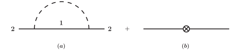
Figure 2: The diagrams for the $D_{2}$ self-energy.

Since Eq. (14) cannot be solved analytically, the on-shell renormalization scheme is not the most convenient choice. A simpler renormalization scheme for the $D_{2}$ mass is to choose the mass counterterm so the self-energy $\Sigma_{2a}(p_{0},0)$ vanishes at the $D_{1}D_{2}$ threshold: $\delta M=-\Sigma_{2a}(M_{1}+m,0)$. The self-energy is then

$$\Sigma(p_{0},p)=-i\frac{g^{2}m_{1}}{2\pi}\left(2m_{1}\left[p_{0}-M_{1}-m-\frac{p^{2}}{2(M_{1}+m)}+i\varepsilon\right]\right)^{1/2}.$$ (18)

With this renormalization prescription, the parameter $M_{2}$ differs at order $g^{4}$ from the physical $D_{2}$ mass, which is given by the real part of the solution to Eq. (14). The width $\Gamma_{2}$, which is given by the imaginary part of the solution to Eq. (14), reduces at leading order in $g$ to $\Gamma_{2}=-2\,{\rm Im}\,\Sigma_{2a}(M_{2},0)$. This agrees with the explicit expression for the decay rate of $D_{2}$ at order $g^{2}$ obtained in Eq. (13). To order $g^{2}$, the wavefunction normalization factor in Eq. (17) is

$$Z_{2}(p)^{-1}=1+i\frac{g^{2}m_{1}^{2}}{2\pi}\Big{(}2m_{1}(M_{2-1}-m)[1-p^{2}/(2(M_{1}+m)M_{2})]\Big{)}^{-1/2}.$$ (19)

Since the momentum $p$ is restricted to the nonrelativistic region, the term $p^{2}/(2(M_{1}+m)M_{2})$ can always be neglected compared to 1. The resulting wavefunction normalization factor is independent of $p$:

$$Z_{2}^{-1}=1+i\frac{g^{2}m_{1}^{2}}{2\pi}\left[2m_{1}(M_{2-1}-m)\right]^{-1/2}.$$ (20)

The correction term is pure imaginary.

II.5 The Complex Mass Scheme

The $D_{2}-D_{1}\phi$ interaction allows a virtual $D_{2}$ whose energy is greater than $M_{1}+m$ to decay into $D_{1}\phi$. In the amplitude for such a process at leading order in $g$, the propagator of the virtual $D_{2}$ diverges. Near such a point in momentum space, the corrections to the $D_{2}$ propagator from higher orders in $g$ are not suppressed. This problem can be solved by summing the $D_{2}$ propagator corrections to all orders. The effect is to add $-\Sigma(p_{0},p)$ to the denominator $p_{0}-p^{2}/(2M_{2})+i\varepsilon$ of the $D_{2}$ propagator. The imaginary part of the self-energy $\Sigma(p_{0},p)$ eliminates any divergence in the $D_{2}$ propagator for real values of the energy. One drawback of this solution is that it leads to unnecessarily complicated expressions for the integrals in loop diagrams with $D_{2}$ propagators.

Summing the $D_{2}$ self-energy corrections to all orders is essential only near the pole in the propagator. In other regions of the energy $p_{0}$, $\Sigma(p_{0},p)$ is a perturbative correction to the denominator of the propagator that is suppressed by a power of $g^{2}$. In those regions, summing the $D_{2}$ propagator corrections to all orders is optional. At the pole in $p_{0}$, the self-energy $\Sigma(p_{0},p)$ reduces to $-i\Gamma_{2}/2$. An alternative resummation that eliminates the divergence in the propagator for real values of the energy without changing the order in $g$ of the truncation error is to sum only the $-i\Gamma_{2}/2$ term in the self-energy to all orders and treat the remainder of the self-energy as a perturbation. An advantage of this partial resummation is that it leads to simpler expressions for the integrals in loop diagrams with $D_{2}$ propagators.

A systematic method for implementing this partial resummation is the complex mass scheme Denner:2006ic . This method has been used in Standard Model calculations at next-to-leading order Denner:2005es ; Denner:2005fg ; Bredenstein:2006rh . The application of this method to the scalar meson model involves adding cancelling terms to the free and interaction terms in the Lagrangian:

$$\Delta{\cal L}_{\rm free} = (i\Gamma_{2}/2)D_{2}^{\dagger}D_{2}+(Z_{2}^{-1}-1)D_{2}^{\dagger}\left(i\frac{\partial}{\partial t}-M_{2}+i\Gamma_{2}/2+\frac{1}{2M_{2}}\nabla^{2}\right)D_{2},$$ (21a)

$$\Delta{\cal L}_{\rm int} = -(i\Gamma_{2}/2)D_{2}^{\dagger}D_{2}-(Z_{2}^{-1}-1)D_{2}^{\dagger}\left(i\frac{\partial}{\partial t}-M_{2}+i\Gamma_{2}/2+\frac{1}{2M_{2}}\nabla^{2}\right)D_{2},$$ (21b)

where $\Gamma_{2}$ is the $D_{2}$ width and $Z_{2}$ is the $D_{2}$ wavefunction normalization factor. To order $g^{2}$, $\Gamma_{2}$ and $Z_{2}$ are given by Eqs. (13) and (20). Since $i\Gamma_{2}/2$ is pure imaginary and $Z_{2}$ is complex, the free Lagrangian consisting of the sum of Eqs. (3) and (21a) corresponds to a nonhermitian Hamiltonian. The effects of the nonhermiticity are cancelled exactly if the interaction terms in Eq. (21b) are calculated to all orders. At any finite order in perturbation theory, the complex mass scheme gives amplitudes that are uniformly accurate to the appropriate order in $g$, even if there is a virtual $D_{2}$ that decays into $D_{1}\phi$. The effect of adding Eq. (21a) to the free Lagrangian in Eq. (3) is to change the $D_{2}$ propagator:

$$\frac{i}{p_{0}-M_{2}-p^{2}/(2M_{2})+i\varepsilon}\longrightarrow\frac{iZ_{2}}{p_{0}-(M_{2}-i\Gamma_{2}/2)-p^{2}/(2M_{2})}.$$ (22)

The effect of adding Eq. (21b) to the interaction Lagrangian in Eq. (4) is to change the counterterm vertex in Fig. 1:

$$-i\delta M\longrightarrow-i(\delta M+i\Gamma_{2}/2)-i(Z_{2}^{-1}-1)\left[p_{0}-M_{2}+i\Gamma_{2}/2-p^{2}/(2M_{2})\right].$$ (23)

It is convenient to also rescale the fields $D_{2}(x)$ and $D_{2}^{\dagger}(x)$ by the same complex factor $Z_{2}^{1/2}$. This eliminates the factor of $Z_{2}$ from the numerator of the $D_{2}$ propagator in Eq. (22). It also multiplies all the interaction terms in Eqs. (4) and (21b) by $Z_{2}$ or $Z_{2}^{1/2}$. Since we will use nonperturbative renormalization for the coupling constant $Z_{2}\lambda_{0}$ for the $D_{1}D_{2}$ contact interaction, the factor of $Z_{2}$ only affects the value of the unphysical bare coupling constant $\lambda_{0}$. Since $Z_{2}=1+O(g^{2})$, the other factors of $Z_{2}$ or $Z_{2}^{1/2}$ in the interaction vertices contribute only at order $g^{4}$ and higher. We will be calculating only to order $g^{2}$, so we will ignore these factors of $Z_{2}$ and $Z_{2}^{1/2}$.

The perturbation expansion in the complex mass scheme corresponds to ordinary perturbation theory in $g$ followed by a resummation to all orders of a subset of terms that are higher order in $g$. We will refer to calculations to order $g^{0}$ in this perturbation expansion as leading order (LO) in the complex mass scheme. We will refer to calculations through order $g^{2}$ in this perturbation expansion as next-to-leading order (NLO) in the complex mass scheme.

II.6 Propagator for $\bm{X}$

We can use the scalar meson model to describe processes with asymptotic states that include not only the particles $D_{1}$ and $\phi$, but also the bound state $X$. The local composite operator $D_{1}^{\dagger}D_{2}^{\dagger}(x)$ has a nonzero amplitude to create $X$ from the vacuum. Thus $D_{1}D_{2}(x)$ can be used as an interpolating field for $X$. It is more convenient to use the operator $\lambda_{0}D_{1}D_{2}(x)$, because this is a renormalized operator whose matrix elements do not depend on the ultraviolet cutoff Braaten:2006sy . The corresponding propagator for $X$ is

$$\Delta_{X}(E,P)=\int d^{4}x\,e^{iP\cdot x}\langle\emptyset|\lambda_{0}D_{1}D_{2}(x)\lambda_{0}D_{1}^{\dagger}D_{2}^{\dagger}(0)|\emptyset\rangle.$$ (24)

The momentum 4-vector in the Fourier transform is $P^{\mu}=(E,\vec{P}\,)$, where $E$ and $\vec{P}\,$ are the energy and momentum of $X$. At $P=0$, this propagator has a pole at the complex energy $E_{\rm pole}$. Near the pole in the energy, the behavior of the propagator at $P=0$ is

$$\Delta_{X}(E,0)\longrightarrow\frac{iZ_{X}}{E-E_{\rm pole}+i\varepsilon}.$$ (25)

The energy $E_{\rm pole}$ determines the binding energy $E_{X}$ and the width $\Gamma_{X}$ of $X$ through Eq. (11). The residue of the pole defines the wavefunction normalization factor $Z_{X}$, which is complex valued. Because the propagator $\Delta_{X}(E,P)$ has mass dimension $-2$, $Z_{X}$ has mass dimension $-1$.

Strictly speaking, since $X$ has a nonzero width $\Gamma_{X}$, there are no T-matrix elements for processes involving $X$ in the initial or final state, because the decay of the $X$ prevents it from being a truly asymptotic state. However if $\Gamma_{X}$ is sufficiently small, the $X$ can propagate over a long time interval before decaying, and it can therefore be treated as a quasi-asymptotic state. We can use the Lehmann-Symanzik-Zimmermann (LSZ) formalism to define T-matrix elements for the $X$ that are closely related to T-matrix elements for decay products of the $X$ whose total energy is tuned to the peak of the $X$ resonance. To define the T-matrix element ${\cal T}$ for a process with $X$ in the initial or final state, we start with a Green’s functions for the operator $\lambda_{0}D_{1}^{\dagger}D_{2}^{\dagger}(x)$ or $\lambda_{0}D_{1}D_{2}(x)$. The connected Green’s function at 4-momentum $(E,\vec{P}\,)$ is amputated by multiplying by the inverse propagator $\Delta_{X}(E,P)^{-1}$, it is normalized by multiplying by $Z_{X}^{1/2}$, and then it is evaluated at the real energy $M_{X}+P^{2}/(2M_{X})$. This gives the T-matrix element multiplied by $i$ for a state $X$ with the standard nonrelativistic normalization. The T-matrix element ${\cal T}$ for a state $X$ with the standard relativistic normalization is obtained by multiplying by $\sqrt{2M_{X}}$.

To justify this prescription, we consider a process $A\to B+C$, where $A$ and $B$ both represent one or more particles and $C$ denotes a set of particles that can be decay products of $X$. The T-matrix for this process will have a resonant enhancement when the invariant mass $M$ of the particles in $C$ is near the mass $M_{X}$. The resonant contribution to the T-matrix element for $A\to B+C$ in the rest frame of $C$ can be approximated by

$$i{\cal T}[A\to B+C]\approx i{\cal T}[A\to B+X]\,\frac{i}{2M_{X}(M-M_{X}+i\Gamma_{X}/2)}\,i{\cal T}[X\to C].$$ (26)

Our prescription for T-matrix elements such as ${\cal T}[A\to B+X]$ and ${\cal T}[X\to C]$ involves evaluating the amputated connected Green’s function at the real energy $E=M_{X}$. This ensures that the expression in Eq. (26) is as good an approximation as possible to the T-matrix element ${\cal T}[A\to B+C]$ near the peak of the resonance.

As a simple illustration of the prescription for T-matrix elements for processes involving $X$, we consider the forward scattering process $X\to X$. The relevant Green’s function in the rest frame of $X$ is the negative of the propagator $\Delta_{X}(E,0)$. This must be multiplied by two factors of $\Delta_{X}(E,0)^{-1}Z_{X}^{1/2}$, one for the $X$ in the inital state and one for the $X$ in the final state. The T-matrix element $i{\cal T}[X\to X]$ is then obtained by evaluating this at $E=M_{X}$ and multiplying it by $2M_{X}$:

$$i{\cal T}[X\to X]=-\frac{2M_{X}Z_{X}}{\Delta_{X}(M_{X},0)}.$$ (27)

II.7 Short-distance production and decay processes

The scalar meson model defined by the lagrangian in Eqs. (3) and (4) can be a low-energy approximation to a more fundamental quantum field theory. The fundamental theory may include high energy processes that can create $D_{1}D_{2}$ or $D_{1}D_{1}\phi$ with invariant mass near $M_{1+2}$. If long-distance effects involving momenta much smaller than $m$ can be separated from short-distance effects involving momenta of order $m$ and larger, we can use the scalar meson model to calculate the long-distance effects. The basic tool required to separate long-distance effects from short-distance effects is the operator product expansion Braaten:2006sy . Applications of the operator product expansion to the scalar meson model at 0^th order in $g$ were described in Ref. Braaten:2006sy . Below, we give the leading terms in the operator product expansions of the T-matrix elements for some of the processes considered in Ref. Braaten:2006sy .

The general production process for $X$ has the form $A\to B+X$, where $A$ and $B$ each represent one or more particles. There can be analogous production processes for $D_{1}D_{1}\phi$. In the case of $D_{1}D_{1}\phi$, we assume that the invariant mass $M$ satisfies the condition in Eq. (8). This implies that the relative momenta of the mesons, which we denote generically by $\vec{p}\,$, are small compared to the natural momentum scale $m$. We call the production process a short-distance process if all the particles in $A$ and $B$ have momenta in the rest frame of $X$ or $D_{1}D_{1}\phi$ that are of order $m$ or larger. The T-matrix element for a short-distance production process can be expanded in powers of the small energy differences $M-M_{1+2}$ and $M_{2-1}-m$ divided by $m^{2}/M_{12}$ and higher energy scales and in powers of the small relative momenta $\vec{p}\,$ divided by $m$ and higher momentum scales. The operator product expansion can be used to organize the expansions of the T-matrix elements into sums of products of short-distance coefficients and matrix elements of local operators between the vacuum state $|\emptyset\rangle$ and the appropriate final state. The leading terms in the expansions are those with the lowest dimension operator, which is $D_{1}^{\dagger}D_{2}^{\dagger}(x)$. The corresponding renormalized operator is $\lambda_{0}D_{1}^{\dagger}D_{2}^{\dagger}(x)$. In Feynman diagrams, the local operator $\lambda_{0}D_{1}^{\dagger}D_{2}^{\dagger}(x)$ is represented by a dot from which a $D_{1}$ line and a $D_{2}$ line emerge, as illustrated in Fig. 3. If we keep only the leading terms, the factorization formulas for the T-matrix elements reduce to

$${\cal T}[A\to B+X] = \sqrt{2M_{X}}\;{\cal C}_{A}^{B,12}\,\langle X|\lambda_{0}D_{1}^{\dagger}D_{2}^{\dagger}(0)|\emptyset\rangle,$$ (28a)

$${\cal T}[A\to B+D_{1}D_{1}\phi] = \sqrt{8M_{1}^{2}m}\;{\cal C}_{A}^{B,12}\,\langle D_{1}D_{1}\phi|\lambda_{0}D_{1}^{\dagger}D_{2}^{\dagger}(0)|\emptyset\rangle.$$ (28b)

The Wilson coefficient ${\cal C}_{A}^{B,12}$ is a function of high energy scales, such as $m$ and $M_{12}$, and of the total momentum of the $X$ or $D_{1}D_{1}\phi$. The only dependence on whether the final state contains $X$ or $D_{1}D_{1}\phi$ is in the matrix elements of the local operator $\lambda_{0}D_{1}^{\dagger}D_{2}^{\dagger}(0)$. Short-distance and long-distance effects are separated in Eqs. (28).

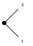
Figure 3: Vertex for the $\lambda_{0}D_{1}D_{2}$ and $\lambda_{0}D_{1}^{\dagger}D_{2}^{\dagger}$ operators.

The decay of $X$ into $D_{1}D_{1}\phi$ can be described within the scalar meson model. The fundamental theory may also allow the decay of $X$ into other final states $C$. We call such a process a short-distance decay if all the particles in $C$ have momenta in the rest frame that are of order $m$ or larger. The T-matrix element for such a process can be expanded in powers of the small energy differences $M_{X}-M_{1+2}$ and $M_{2-1}-m$ divided by $m^{2}/M_{12}$ and higher energy scales. The operator product expansion can be used to organize the expansion of the T-matrix element into sums of products of short-distance coefficients and matrix elements of local operators between the state $|X\rangle$ and the vacuum state. The leading term in the expansion is the one with the lowest dimension operator, which is $D_{1}D_{2}(x)$. The corresponding renormalized operator is $\lambda_{0}D_{1}D_{2}(x)$. If we keep only this term, the factorization formula for the T-matrix element reduces to

$${\cal T}[X\to C]=\sqrt{2M_{X}}\;{\cal C}_{12}^{C}\,\langle\emptyset|\lambda_{0}D_{1}D_{2}(0)|X\rangle.$$ (29)

The Wilson coefficient ${\cal C}_{12}^{C}$ is a function of high energy scales, such as $m$ and $M_{12}$. Short-distance and long-distance effects are separated in Eqs. (29).

If the fundamental theory includes processes that allow the production of $X$ via $A\to B+X$ and the decay of $X$ via $X\to C$, it also allows the process $A\to B+C$, where $C$ represents the same particles but with a variable invariant mass $M$ instead of $M_{X}$. This process has a resonant enhancement when $M$ is near the $D_{1}D_{2}$ threshold as specified by Eq. (8). We call it a short-distance process if each of the particles in $A$ and $B$ has momentum large compared to $m$ in the rest frame of $C$ and if the relative momentum between each particle in $C$ and each particle in $A$ or $B$ is large compared to $m$. The T-matrix element for such a process can be described within the scalar meson model by a double operator product expansion. The leading terms in this expansion are

$${\cal T}[A\to B+C] = {\cal C}_{A}^{B,\,C}+{\cal C}_{A}^{B,12}{\cal C}_{12}^{C}\int d^{4}x\,e^{iP\cdot x}\langle\emptyset|\lambda_{0}D_{1}D_{2}(x)\lambda_{0}D_{1}^{\dagger}D_{2}^{\dagger}(0)|\emptyset\rangle,$$ (30)

where the 4-vector is $P^{\mu}=(M,\vec{0}\,)$. The Wilson coefficients ${\cal C}_{A}^{B,12}$ and ${\cal C}_{12}^{C}$ are the same ones that appear in the operator product expansions in Eqs. (28) and (29). The first term ${\cal C}_{A}^{B,C}$ on the right side of Eq. (30) takes into account the direct production of $C$ at short distances. This term can be expanded in powers of the small energy differences $M-M_{1+2}$ and $M_{2-1}-m$ divided by energy scales of order $m^{2}/M_{12}$ or higher. The leading term in this expansion is simply a constant. According to Eq. (24), the Fourier transform in Eq. (30) is just the $X$ propagator evaluated at $E=M$. Short-distance and long-distance effects are not yet separated in Eq. (30), because the $X$ propagator requires an additive renormalization Braaten:2006sy .

III Leading order in $\bm{g}$

At $0^{\rm th}$ order in $g$, the only interaction in the scalar meson model is the contact interaction between $D_{1}$ and $D_{2}$ with coupling constant $\lambda_{0}$. The $D_{1}D_{1}\phi$ states remain noninteracting at this order in $g$. In this section, we summarize some of the results at $0^{\rm th}$ order in $g$ that were obtained in Ref. Braaten:2006sy and we generalize those results to the complex mass scheme.

III.1 Amplitude for $\bm{D_{1}D_{2}\to D_{1}D_{2}}$

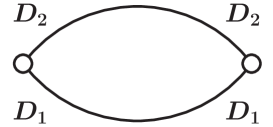
Figure 4: Diagram of order $g^{0}$ for the amplitude for the propagation of $D_{1}D_{2}$ between contact interactions. The open dots indicate that the vertex factors $-i\lambda_{0}$ are omitted.

At 0^th order in $g$, all the observables for processes near the $D_{1}D_{2}$ threshold are related in a simple way to the connected Green’s function for $D_{1}D_{2}\to D_{1}D_{2}$. The basic building block for this Green’s function is the amplitude $iL_{0}(E)$ for the propagation of the $D_{1}D_{2}$ pair between successive contact interactions, which is given by the Feynman diagram in Fig. 4. The amplitude $L_{0}(E)$ is calculated in Section A.3 of the Appendix. The analytic expression using dimensional regularization is given in Eq. (106). The result in a general regularization scheme is

$$L_{0}(E)=L_{0}(M_{1+2})+\frac{M_{12}}{2\pi}\kappa(E),$$ (31)

where $\kappa(E)$ is the energy variable defined by

$$\kappa(E)=\sqrt{-2M_{12}(E-M_{1+2})-i\varepsilon}.$$ (32)

This variable vanishes at the $D_{1}D_{2}$ threshold $E=M_{1+2}$. It is real and positive if $E<M_{1+2}$ and it is pure imaginary with a negative imaginary part if $E>M_{1+2}$. The term $L_{0}(M_{1+2})$ in Eq. (31) is real valued and includes a linear ultraviolet divergence.

The amputated connected Green’s function $i\mathcal{A}_{0}(E)$ for $D_{1}D_{2}\to D_{1}D_{2}$ can be calculated nonperturbatively by summing the geometric series represented by Fig. 5 to all orders in $\lambda_{0}$:

$$i\mathcal{A}_{0}(E)=\frac{-i}{1/\lambda_{0}-L_{0}(E)}.$$ (33)

The renormalization prescription for $\lambda_{0}$ specified by Eq. (10) is that ${\rm Re}\,\mathcal{A}_{0}^{-1}(E)$ must vanish at $M_{1+2}-\kappa_{X}^{2}/(2M_{12})$. This requires the inverse bare coupling constant to be

$$\frac{1}{\lambda_{0}}=L_{0}(M_{1+2})+\frac{M_{12}}{2\pi}\kappa_{X}.$$ (34)

Using this expression for $1/\lambda_{0}$ and the expression for $L_{0}(E)$ in Eq. (106), the amplitude in Eq. (33) reduces to

$$\mathcal{A}_{0}(E)=\frac{2\pi/M_{12}}{\kappa(E)-\kappa_{X}}.$$ (35)

If we were to use the complex mass scheme, the amplitude $L_{0}(E)$ would be given by Eq. (31) with $M_{1+2}$ replaced by $M_{1+2}-i\Gamma_{2}/2$. If we again demand that ${\rm Re}\,\mathcal{A}_{0}^{-1}(E)$ must vanish at $M_{1+2}-\kappa_{X}^{2}/(2M_{12})$, the renormalized expression for the amplitude would be

$$\mathcal{A}_{0}(E)=\frac{2\pi/M_{12}}{\gamma(E)-{\rm Re}\,\gamma_{X}},$$ (36)

where $\gamma(E)$ is a complex energy variable defined by

$$\gamma(E)=\sqrt{-2M_{12}(E-M_{1+2}+i\Gamma_{2}/2)}$$ (37)

and $\gamma_{X}$ is its value at $E=M_{1+2}-\kappa_{X}^{2}/(2M_{12})$:

$$\gamma_{X}=\sqrt{\kappa_{X}^{2}-iM_{12}\Gamma_{2}}.$$ (38)

The variable $\gamma(E)$ vanishes at the complex threshold $E=M_{1+2}-i\Gamma/2$ and it has a negative imaginary part for all real values of $E$.

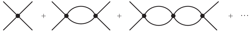
Figure 5: The connected Green’s function $i\mathcal{A}_{0}(E)$ for $D_{1}D_{2}\to D_{1}D_{2}$ at $0^{\textrm{th}}$ order in $g$ can be obtained by summing a geometric series of one-loop diagrams.

III.2 Propagator for $\bm{X}$

If the local composite operator $\lambda_{0}D_{1}D_{2}(x)$ is used as an interpolating field for $X$, the propagator for $X$ is given in Eq. (24). The diagrams for the propagator of $X$ at 0^th order in $g$ are shown in Fig. 6. These diagrams form a geometric series whose sum in the rest frame $\vec{P}=0$ is

$$\Delta_{X}(E,0)=\frac{i\lambda_{0}^{2}L_{0}(E)}{1-\lambda_{0}L_{0}(E)}.$$ (39)

Using the expression for $\mathcal{A}_{0}(E)$ in Eq. (33), we can express the propagator for $X$ as

$$\Delta_{X}(E,0)=-i[\lambda_{0}+\mathcal{A}_{0}(E)].$$ (40)

To obtain a renormalized propagator for $X$ that does not depend on the ultraviolet cutoff, an additive renormalization is necessary. After adding the constant $i\lambda_{0}$, we obtain the renormalized propagator $-i\mathcal{A}_{0}(E)$.

Figure 6: Feynman diagrams for the $X$ propagator at 0^th order in $g$. The interpolating field for the $X$ is $\lambda_{0}D_{1}D_{2}$.

The term $-i\mathcal{A}_{0}(E)$ in the propagator for $X$ in Eq. (40) has a pole at the complex energy $E_{\rm pole}$ given in Eq. (11). Using the renormalized expression for $\mathcal{A}_{0}(E)$ in Eq. (35), we find that the binding energy and width of $X$ at 0^th order in $g$ are

$$E_{X} = \kappa_{X}^{2}/(2M_{12}),$$ (41a)

$$\Gamma_{X} = 0.$$ (41b)

The wavefunction normalization factor for $X$ is

$$Z_{X}=\frac{2\pi}{M^{2}_{12}}\kappa_{X}.$$ (42)

If we were to use the complex mass scheme, the amplitude $\mathcal{A}_{0}(E)$ would be given by Eq. (36). This amplitude has a pole at a complex energy $E_{\rm pole}$ that determines the binding energy and width of $X$. The complex parameter $E_{\rm pole}$ satisfies

$$\gamma(E_{\rm pole})-{\rm Re}\,\gamma_{X}=0,$$ (43)

where $\gamma(E)$ and $\gamma_{X}$ are defined in Eqs. (37) and (38). Comparing with Eq. (11), we find that at LO in the complex mass scheme, the binding energy and width of $X$ are

$$E_{X} = ({\rm Re}\,\gamma_{X})^{2}/(2M_{12}),$$ (44a)

$$\Gamma_{X} = \Gamma_{2}.$$ (44b)

If we treat $\Gamma_{2}$ as being of order $g^{2}$, the binding energy of $X$ in Eq. (44a) differs from $\kappa_{X}^{2}/(2M_{12})$ only at order $g^{4}$. The wavefunction normalization constant for $X$ at LO in the complex mass scheme is

$$Z_{X}=\frac{2\pi}{M^{2}_{12}}\,{\rm Re}\,\gamma_{X}.$$ (45)

III.3 Short-distance Production of $\bm{X}$

The operator product expansion of the T-matrix element for a short-distance production process $A\to B+X$ is given in Eq. (28a). The vacuum–to–$X$ matrix element can be calculated via the LSZ formalism using $\lambda_{0}D_{1}D_{2}(x)$ as an interpolating field for $X$ Braaten:2006sy :

$$\langle X|\lambda_{0}D_{1}^{\dagger}D_{2}^{\dagger}(0)|\,\emptyset\rangle=Z_{X}^{1/2}.$$ (46)

At 0^th order in $g$, the normalization constant $Z_{X}$ is given in Eq. (42). At LO in the complex mass scheme, $Z_{X}$ is given in Eq. (45). The T-matrix element in Eq. (28a) can be expressed as the product of a short-distance factor and a long-distance factor:

$${\cal T}[A\to B+X]=\sqrt{2M_{X}}\,{\cal C}_{A}^{B,12}\,Z_{X}^{1/2}.$$ (47)

The rate for producing $X$ is obtained by squaring the T-matrix element in Eq. (47) and integrating over the appropriate phase space. If $A$ consists of a single particle, its decay rate into $B+X$ can be expressed in the factored form

$$\Gamma[A\to B+X]=\Gamma_{A}^{B}\,M_{12}|Z_{X}|.$$ (48)

We have followed Ref. Braaten:2006sy in choosing the long-distance factor in Eq. (48) to be $M_{12}|Z_{X}|$, which is dimensionless. The short-distance factor $\Gamma_{A}^{B}$ is

$$\Gamma_{A}^{B} = \frac{M_{1+2}}{M_{A}M_{12}}\int\frac{d^{3}P}{(2\pi)^{3}2E}\int\prod_{i\in B}\frac{d^{3}p_{i}}{(2\pi)^{3}2E_{i}}\left|{\cal C}_{A}^{B,12}\right|^{2}(2\pi)^{4}\delta^{(4)}(P_{A}-P-\mbox{$\sum\limits_{i\in B}$}\,p_{i}),$$ (49)

where the 4-vector $P^{\mu}$ satisfies $P^{2}=M_{1+2}^{2}$.

III.4 Short-distance Decay of $\bm{X}$

The operator product expansion of the T-matrix element for a short-distance decay process $X\to C$ is given in Eq. (29). The $X$–to–vacuum matrix element can be calculated via the LSZ formalism using $\lambda_{0}D_{1}^{\dagger}D_{2}^{\dagger}(x)$ as an interpolating field for $X$ Braaten:2006sy :

$$\langle\emptyset|\lambda_{0}D_{1}D_{2}(0)|X\rangle=Z_{X}^{1/2}.$$ (50)

At 0^th order in $g$, the normalization constant $Z_{X}$ is given in Eq. (42). At LO in the complex mass scheme, $Z_{X}$ is given by Eq. (45). The T-matrix element in Eq. (29) can be expressed as the product of a short-distance factor and a long-distance factor:

$${\cal T}[X\to C]=\sqrt{2M_{X}}\,{\cal C}_{12}^{C}\,Z_{X}^{1/2}.$$ (51)

The decay rate of $X$ into the particles represented by $C$ is obtained by squaring the T-matrix element in Eq. (51) and integrating over the phase space of those particles. It can be expressed in the factored form

$$\Gamma[X\to C]=\Gamma^{C}\,M_{12}|Z_{X}|.$$ (52)

We have followed Ref. Braaten:2006sy in choosing the long-distance factor to be $M_{12}|Z_{X}|$, which is dimensionless. The short-distance factor $\Gamma^{C}$ is

$$\Gamma^{C}=\frac{1}{M_{12}}\int\prod_{j\in C}\frac{d^{3}p_{j}}{(2\pi)^{3}2E_{j}}\left|{\cal C}^{C}_{12}\right|^{2}(2\pi)^{4}\delta^{(4)}\!(P-\mbox{$\sum\limits_{j\in C}$}p_{j}).$$ (53)

where the 4-vector $P^{\mu}$ satisfies $P^{2}=M_{1+2}^{2}$.

III.5 Line shape of $\bm{X}$ in a Short-distance Decay Channel

If $X$ can be produced via the short-distance process $A\to B+X$ and if it can decay via the short-distance process $X\to C$, then there can be resonant enhancement of the process $A\to B+C$, where $C$ represents the same particles but with a variable invariant mass $M$ instead of $M_{X}$. The T-matrix element for this process can be expressed as the double operator product expansion in Eq. (30). The Fourier transform of the matrix element is just the $X$ propagator evaluated at $(E,\vec{P}\,)=(M,\vec{0}\,)$. The T-matrix element therefore reduces to

$${\cal T}[A\to B+C] = {\cal C}_{A}^{B,C}+{\cal C}_{A}^{B,12}{\cal C}_{12}^{C}\frac{i\lambda_{0}^{2}L_{0}(M)}{1-\lambda_{0}L_{0}(M)}.$$ (54)

The T-matrix element can be expressed in a form in which the short-distance effects and long-distance effects are separated:

$${\cal T}[A\to B+C] = -i{\cal C}_{A}^{B,12}{\cal C}_{12}^{C}\left[\mathcal{A}_{0}(M)-(2\pi/M_{12})c_{A}^{B,C}\right],$$ (55)

where $\mathcal{A}_{0}(E)$ is given in Eq. (35) and $c_{A}^{B,C}$ is a complex constant with dimensions of length that is completely determined by short-distance factors:

$$c_{A}^{B,C} = -i\frac{M_{12}({\cal C}_{A}^{B,C}-i\lambda_{0}{\cal C}_{A}^{B,12}{\cal C}_{12}^{C})}{2\pi{\cal C}_{A}^{B,12}{\cal C}_{12}^{C}}.$$ (56)

The nonresonant term $c_{A}^{B,C}$ in Eq. (55) is a combination of short-distance factors, so the natural scale for $c_{A}^{B,C}$ is $1/m$. The condition $\kappa_{X}\ll m$ and the condition on $M$ in Eq. (8) imply that the nonresonant term in Eq. (55) is small compared to the resonant term in the threhsold region secified by Eq. (8). We therefore set $c_{A}^{B,C}=0$.

The invariant mass distribution of the particles in $C$ is obtained by squaring the T-matrix element and integrating over the momenta of all the particles in the final state. If $A$ consists of a single heavy particle, the invariant-mass distribution of the particles in $C$ has the form

$$\frac{d\Gamma}{dM}[A\to B+C] = \big{(}\Gamma_{A}^{B}\Gamma^{C}\big{)}\,\frac{M_{12}^{2}}{2\pi}\left|\mathcal{A}_{0}(M)\right|^{2}.$$ (57)

The short-distance factors $\Gamma_{A}^{B}$ and $\Gamma^{C}$ are the same as in Eqs. (48) and (52). At 0^th order in $g$, $\mathcal{A}_{0}(E)$ is given in Eq. (35). At LO in the complex mass scheme, $\mathcal{A}_{0}(E)$ is given in Eq. (36). Note that if the invariant mass distribution in Eq. (57) is divided by the product of the decay rates $\Gamma[A\to B+X]$ and $\Gamma[X\to C]$ in Eqs. (48) and (52), the short-distance factors cancel. This combination of observables has only a long-distance factor given by $|\mathcal{A}_{0}(M)|^{2}/(2\pi|Z_{X}|^{2})$.

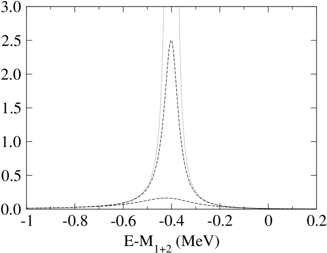
Figure 7: Line shapes $|\mathcal{A}_{0}(E)|^{2}$ of the $X$ resonance in a short-distance decay channel at leading order in $g$. The dotted line is at order $g^{0}$ in ordinary perturbation theory (using $\mathcal{A}_{0}(E)$ in Eq. (35)). The dashed lines are at LO in the complex mass scheme (using $\mathcal{A}_{0}(E)$ in Eq. (36)). The line shapes are shown for $\kappa_{X}=27.8$ MeV and for both $\Gamma_{2}=0.07$ MeV (upper solid line) and $\Gamma_{2}=0.28$ MeV (lower solid line). The units on the vertical axis are $10^{-5}\ {\rm MeV}^{-4}$.

The line shape of $X$ as a function of the invariant mass $E$ of the particles in $C$ is given by the factor $|\mathcal{A}_{0}(E)|^{2}$ in Eq. (57). In Fig. 7, we compare the line shapes at 0^th order in $g$ and at LO in the complex mass scheme. At 0^th order in $g$, the line shape diverges at $M_{1+2}-\kappa_{X}^{2}/(2M_{12})$. In the complex mass scheme, the line shape is a resonance whose maximum is near $M_{1+2}-\kappa_{X}^{2}/(2M_{12})$ and whose width is determined by $\Gamma_{2}$. If $\Gamma_{2}\ll\kappa_{X}^{2}/(2M_{12})$, the line shape for $|E-M_{1+2}+\kappa_{X}^{2}/(2M_{12})|\ll\kappa_{X}^{2}/(2M_{12})$ is a nonrelativistic Breit-Wigner resonance whose full width at half-maximum is $\Gamma_{2}$:

$$\left|\mathcal{A}_{0}(E)\right|^{2}\approx\frac{4\pi^{2}\kappa_{X}^{2}/M_{12}^{4}}{[E-M_{1+2}+\kappa_{X}^{2}/(2M_{12})]^{2}+\Gamma_{2}^{2}/4}.$$ (58)

However, a Breit-Wigner resonance has tails that fall off like $E^{-2}$ and it is integrable. In contrast, the line shape $|\mathcal{A}_{0}(E)|^{2}$ with $\mathcal{A}_{0}(E)$ given by Eq. (36) has tails that fall off only like $E^{-1}$ and it is therefore not integrable. Thus the area under the resonance is not as well-defined as for a Breit-Wigner resonance.

IV Second Order in $\bm{g}$

In this section, we calculate the results in Section III to next-to-leading order in $g$. Since the $D_{2}-D_{1}\phi$ interaction allows transitions to $D_{1}D_{1}\phi$ states, we also calculate the rates for processes whose final state includes $D_{1}D_{1}\phi$.

IV.1 Amplitude for $\bm{D_{1}D_{2}\to D_{1}D_{2}}$

One of the basic building blocks for the amplitudes for processes near the $D_{1}D_{2}$ threshold is the amplitude for the propagation of $D_{1}D_{2}$ between contact interactions. The term in this amplitude of order $g^{0}$, $iL_{0}(E)$, is given in Eq. (31). The term of order $g^{2}$, $iL_{2}(E)$, is the sum of the three Feynman diagrams in Fig. 8. These diagrams are calculated in Section A.4 of the Appendix. The final expression for $L_{2}(E)$ is the sum of the amplitudes $L_{2a}(E)$ and $L_{2b}(E)$ given by Eqs. (114) and (122):

$$L_{2}(E)=L_{2}(2M_{1}+m)+\frac{M_{12}}{2\pi}F(\kappa(E)),$$ (59)

where $\kappa(E)$ is the energy variable defined in Eq. (32), the function $F(\kappa)$ is

$$F(\kappa) = \frac{g^{2}M_{12}m_{1}}{\pi^{2}}\Bigg{[}2\int_{0}^{1}\frac{dz}{z^{2}}\left(\frac{t^{3}(z)}{1-t(z)}\right)^{1/2}\ln\frac{z\kappa^{2}+(1-z)(m_{1}/M_{12})(\kappa^{2}-\kappa_{1}^{2})}{z\kappa_{1}^{2}}$$ (60)

$$\hskip 56.9055pt-\left(\frac{m_{1}}{M_{12}}\right)^{1/2}\,\left(2\ln\frac{\kappa+\kappa_{1}}{2\kappa_{1}}+\frac{(\kappa-\kappa_{1})^{2}}{2\kappa_{1}\kappa}\ln\frac{\kappa+\kappa_{1}}{\kappa-\kappa_{1}}\right)\Bigg{]},$$

and $\kappa_{1}$ is the value of $\kappa(E)$ at the $D_{1}D_{1}\phi$ threshold $2M_{1}+m$:

$$\kappa_{1} = [2M_{12}(M_{2-1}-m)]^{1/2}.$$ (61)

The function $t(z)$ in the integrand in Eq. (60) is a rational function of $z$ that increases from 0 to 1 as $z$ increases from 0 to 1:

$$t(z)=\frac{z^{2}}{(2-z)^{2}-4(m_{1}/m)^{2}(1-z)^{2}}.$$ (62)

The term $L_{2}(2M_{1}+m)$ in Eq. (59) is real valued and includes logarithmic ultraviolet divergences. The function $F(\kappa)$ vanishes at the $D_{1}D_{1}\phi$ threshold $\kappa=\kappa_{1}$ by definition. The first few terms in the Laurent expansion of $F(\kappa)$ around the $D_{1}D_{2}$ threshold at $\kappa=0$ can be obtained from Eqs. (117) and (124). The leading term is

$$F(\kappa)\longrightarrow-i\frac{g^{2}M_{12}^{2}(m_{1}/M_{12})^{3/2}\kappa_{1}}{2\pi\kappa}.$$ (63)

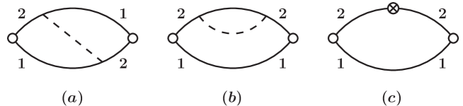
Figure 8: Diagrams of order $g^{2}$ for the amplitude for the propagation of $D_{1}D_{2}$ between contact interactions. The open dots indicate that the vertex factors $-i\lambda_{0}$ are omitted.

At 0^th order in $g$, the ultraviolet divergence in $L_{0}(E)$ was eliminated by summing a geometric series in $L_{0}$ and then renormalizing the coupling constant $\lambda_{0}$. The ultraviolet divergence in $L_{2}(E)$ can be eliminated in a similar way. The geometric series of diagrams that must be summed are those that can be obtained by replacing each one-loop subdiagram in Fig. 5 by the sum of the one-loop subdiagram and the three diagrams for $L_{2}(E)$ in Fig. 8. The sum of that geometric series gives an amplitude $i\mathcal{A}_{2}(E)$ that can be obtained by making the substitution $L_{0}\to L_{0}+L_{2}$ in Eq. (33):

$$i\mathcal{A}_{2}(E)=\frac{-i}{1/\lambda_{0}-[L_{0}(E)+L_{2}(E)]}.$$ (64)

Our renormalization prescription for $\lambda_{0}$ in Eq. (10) requires ${\rm Re}\,\mathcal{A}_{2}^{-1}(E)$ to vanish at $M_{1+2}-\kappa_{X}^{2}/(2M_{12})$. Using this prescription, the amplitude in Eq. (64) can be expressed as

$$\mathcal{A}_{2}(E) = \frac{2\pi/M_{12}}{\kappa(E)+F(\kappa(E))-{\rm Re}\,[\kappa_{X}+F(\kappa_{X}-i\epsilon)]}.$$ (65)

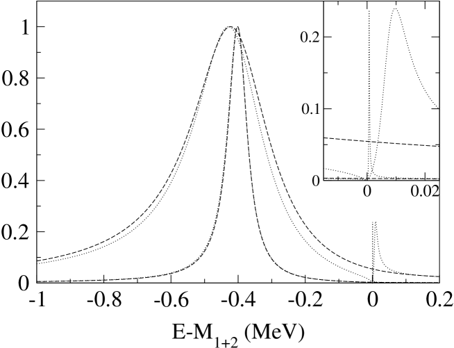
Figure 9: Line shapes $|\mathcal{A}(E)|^{2}$ of the $X$ resonance in a short-distance decay channel. The dotted lines are at order $g^{2}$ in ordinary perturbation theory (using $\mathcal{A}_{2}(E)$ in Eq. (65)). The dashed lines are at LO in the complex mass scheme (using $\mathcal{A}_{0}(E)$ in Eq. (36)). The line shapes are shown for $\kappa_{X}=27.8$ MeV and for both $\Gamma_{2}=0.07$ MeV (the two narrower resonances that are almost indistinguishable) and for $\Gamma_{2}=0.28$ MeV (the two wider resonances). The line shapes are normalized so their maximum values are 1. The inset shows their behavior near the $D_{1}D_{2}$ threshold.

The quantity $|\mathcal{A}_{2}(E)|^{2}$ with $\mathcal{A}_{2}(E)$ given in Eq. (65) is the line shape of the $X$ resonance in a short-distance decay channel to order $g^{2}$ in ordinary perturbation theory. In Fig. 9, we compare this line shape with that at LO in the complex mass scheme, which is $|\mathcal{A}_{0}(E)|^{2}$ with $\mathcal{A}_{0}(E)$ given by Eq. (36). They are shown for two values of the coupling constant $g$ that correspond to the width of $D_{2}$ being $\Gamma_{2}=0.07$ MeV and $0.28$ MeV. The two line shapes have the same qualitative behavior below the resonance and near the peak of the resonance. They have qualitatively different behavior near the $D_{1}D_{2}$ threshold $E=M_{1+2}$. Unlike $|\mathcal{A}_{0}(E)|^{2}$, the function $|\mathcal{A}_{2}(E)|^{2}$ vanishes at the $D_{1}D_{2}$ threshold and has a sharp peak just above the threshold. The inset in Fig. 9 shows the behavior near the $D_{1}D_{2}$ threshold, which is clearly unphysical.

The reason $|\mathcal{A}_{2}(E)|^{2}$ vanishes at the $D_{1}D_{2}$ threshold can be seen from the Laurent expansion of $F(\kappa)$ around $\kappa=0$. The leading term, which is given in Eq. (63), diverges like $1/\kappa$ as $E\to M_{1+2}$. No matter how small the coupling constant $g$, the term proportional to $g^{2}/\kappa$ cannot be treated as a perturbation in the region near $\kappa=0$. The resolution of the problem can be found by noting that the diverging term in Eq. (63) can be expressed as

$$F(\kappa) \longrightarrow -i\frac{M_{12}\Gamma_{2}}{2\kappa},$$ (66)

where $\Gamma_{2}$ is the width of the $D_{2}$ from its decay into $D_{1}\phi$, which is given in Eq. (13). Thus the divergence at $\kappa=0$ implies that near the $D_{1}D_{2}$ threshold, the imaginary part of the $D_{2}$ self-energy must be resummed to all orders. That resummation shifts the branch point in the leading order amplitude from the real threshold $E=M_{1+2}$ to the complex threshold $E=M_{1+2}-i\Gamma_{2}/2$. Making this change and then imposing our renormalization scheme, the amplitude in Eq. (65) becomes

$$\mathcal{A}_{2}(E)\approx\frac{2\pi/M_{12}}{\gamma(E)+F(\kappa(E))+iM_{12}\Gamma_{2}/(2\kappa)-{\rm Re}[\gamma_{X}+F(\kappa_{X}-i\epsilon)]},$$ (67)

where $\gamma(E)$ and $\gamma_{X}$ are defined in Eqs. (37) and (38). This amplitude is a smooth function of $E$ at $\kappa=0$.

A convenient way to implement the resummation in Eq. (67) that can be extended staightforwardly to higher orders in $g$ is to use the complex mass scheme. This automatically gives an amplitude $\mathcal{A}_{2}(E)$ that has smooth behavior at the $D_{1}D_{2}$ threshold and is correct through relative order $g^{2}$. In the complex mass scheme, the contribution to $L_{2}(E)$ from the diagrams in Figs. 8(a) and 8(b) are obtained by replacing the energy variable $\kappa(E)$ by $\gamma(E)$ defined in Eq. (37) and by replacing $\kappa_{1}$ by $\gamma_{1}$, which is the value of $\gamma(E)$ at the $D_{1}D_{1}\phi$ threshold $2M_{1}+m$:

$$\gamma_{1} = \left[2M_{12}(M_{2-1}-m-i\Gamma_{2}/2)\right]^{1/2}.$$ (68)

In the complex mass scheme, there are additional contributions to the function $L_{2}(E)$ coming from the one-loop diagram in Fig. 8(c) with the counterterm vertex in Eq. (21b). The additional contributions are given in Eq. (126). Adding those terms is equivalent to making the substitution

$$F(\kappa)\longrightarrow F(\kappa)+\frac{iM_{12}\Gamma_{2}}{2\kappa}+(Z_{2}^{-1}-1)\left(\frac{2\pi}{M_{12}}L_{0}(M_{1+2})+\kappa\right).$$ (69)

Using the expressions to order $g^{2}$ for $\Gamma_{2}$ in Eq. (13) and $Z_{2}^{-1}$ in Eq. (20), we can see that the additional terms in Eq. (69) cancel the $\kappa^{-1}$ and $\kappa$ terms coming from the Laurent expansions of $L_{2b}(E)$ in Eq. (124). Our renormalization prescription for $\lambda_{0}$ in Eq. (10) requires ${\rm Re}\,\mathcal{A}_{2}^{-1}(E)$ to have a zero at $M_{1+2}-\kappa_{X}^{2}/(2M_{12})$. Using this prescription, the amplitude can be expressed as

$$\mathcal{A}_{2}(E) = \frac{2\pi/M_{12}}{\gamma(E)+F_{\rm cms}(\gamma(E))-{\rm Re}\,[\gamma_{X}+F_{\rm cms}(\gamma_{X})]},$$ (70)

where $\gamma(E)$ and $\gamma_{X}$ are given by Eqs. (37) and (38) and the function $F_{\rm cms}(\gamma)$ is

$$F_{\rm cms}(\gamma) = \frac{g^{2}M_{12}m_{1}}{\pi^{2}}\Bigg{[}2\int_{0}^{1}\frac{dz}{z^{2}}\left(\frac{t^{3}(z)}{1-t(z)}\right)^{1/2}\left(\ln\frac{(1-z)(m_{1}/M_{12})(\gamma_{1}^{2}-\gamma^{2})-z\gamma^{2}}{(1-z)(m_{1}/M_{12})\gamma_{1}^{2}}-i\pi\right)$$ (71)

$$\hskip 56.9055pt-\left(\frac{m_{1}}{M_{12}}\right)^{1/2}\,\left(2\ln\frac{\gamma_{1}+\gamma}{\gamma_{1}}+\frac{(\gamma_{1}-\gamma)^{2}}{2\gamma_{1}\gamma}\ln\frac{\gamma_{1}+\gamma}{\gamma_{1}-\gamma}-1-i\pi\right)\Bigg{]}.$$

The function $F_{\rm cms}(\gamma)$ can be obtained from $F(\kappa)$ in Eq. (60) by subtracting several terms in the Laurent expansion in $\kappa$ and then replacing $\kappa(E)$ and $\kappa_{1}$ by $\gamma(E)$ and $\gamma_{1}$. The terms that are subtracted are the imaginary term of order $\kappa^{-1}$, the real terms of order $\kappa^{0}$, and the imaginary term of order $\kappa$ in the second of the two terms on the right side of Eq. (60). The real terms of order $\kappa^{0}$ are subtracted because they would cancel in the denominator in Eq. (70) anyway. The leading terms in the Laurent expansion of $F_{\rm cms}(\gamma)$ around the complex $D_{1}D_{2}$ threshold at $\gamma=0$ are

$$F_{\rm cms}(\gamma) \longrightarrow \frac{ig^{2}M_{12}m_{1}}{\pi}\Bigg{[}-\frac{m}{m_{1}}\arcsin\frac{m_{1}}{m}+\left(\frac{m_{1}}{M_{12}}\right)^{1/2}+2\left(\frac{M_{12}}{m_{1}}\right)^{1/2}\frac{\gamma}{\gamma_{1}}\Bigg{]}.$$ (72)

For real values of $E$, there is an ambiguity in the function $F_{\rm cms}(\gamma(E))$ in Eq. (70) for $E<2M_{1}+m$ because of the branch point at $\gamma=\gamma_{1}$ in Eq. (71). This ambiguity can be resolved by the substitution $\gamma\to\gamma-i\epsilon$.

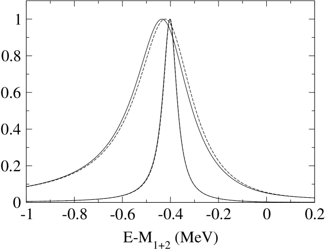
Figure 10: Line shapes $|\mathcal{A}(E)|^{2}$ of the $X$ resonance in a short-distance decay channel using the complex mass scheme. The dashed lines are at LO in the complex mass scheme (using $\mathcal{A}_{0}(E)$ in Eq. (36)). The solid lines are at NLO in the complex mass scheme (using $\mathcal{A}_{2}(E)$ in Eq. (70)). The line shapes are shown for $\kappa_{X}=27.8$ MeV and for both $\Gamma_{2}=0.07$ MeV (the two narrower resonances that are almost indistiguishable) and for $\Gamma_{2}=0.28$ MeV (the two wider resonances). The line shapes are normalized so their maximum values are 1.

In Fig. 10, we compare the line shapes of $X$ in a short-distance decay channel at NLO in the complex mass scheme, which is $|\mathcal{A}_{2}(E)|^{2}$ with $\mathcal{A}_{2}(E)$ given by Eq. (70), and that at LO in the complex mass scheme, which is $|\mathcal{A}_{0}(E)|^{2}$ with $\mathcal{A}_{0}(E)$ given by Eq. (36). They are shown for two values of the coupling constant $g$ that correspond to the width of $D_{2}$ being $\Gamma_{2}=0.07$ MeV and $0.28$ MeV. The curves are normalized so their maximum values are 1. The line shapes at LO and NLO have the same qualitative behavior. As $g$ decreases, the quantitative differences between the line shapes at LO and NLO decrease. Thus the complex mass scheme seems to provide a good solution to the infrared problem near the $D_{1}D_{2}$ threshold that arises in ordinary perturbation theory. We will therefore use the complex mass scheme in most of the calculations in the remainder of this Section.

IV.2 Propagator for $\bm{X}$

If the local composite operator $\lambda_{0}D_{1}D_{2}(x)$ is used as the interpolating field for $X$, the propagator for $X$ is defined in Eq. (24). The expression for the propagator at 0^th in $g$ is given in Eq. (39). A renormalizable expression for the $X$ propagator that is accurate to order $g^{2}$ can be obtained simply by making the substitution $L_{0}\to L_{0}+L_{2}$ in Eq. (39):

$$\Delta_{X}(E,0)=\frac{i\lambda_{0}^{2}[L_{0}(E)+L_{2}(E)]}{1-\lambda_{0}[L_{0}(E)+L_{2}(E)]}.$$ (73)

Comparing with the expression for the amplitude $\mathcal{A}_{2}(E)$ in Eq. (64), we see that the propagator in Eq. (73) can be expressed as

$$\Delta_{X}(E,0)=-i[\lambda_{0}+\mathcal{A}_{2}(E)].$$ (74)

The expression for $\mathcal{A}_{2}(E)$ at NLO in the complex mass scheme is given in Eq. (70). This amplitude has a pole at a complex energy $E_{\rm pole}$ that determines the binding energy and the width of $X$. The energy $E_{\rm pole}$ is the solution to

$$\gamma(E_{\rm pole})+F_{\rm cms}(\gamma(E_{\rm pole}))-{\rm Re}\,[\gamma_{X}+F_{\rm cms}(\gamma_{X})]=0,$$ (75)

where $\gamma(E)$ and $\gamma_{X}$ are defined in Eqs. (37) and (38). The wavefunction normalization constant for $X$ is

$$Z_{X}=\frac{2\pi}{M_{12}^{2}}\frac{{\rm Re}\,\gamma(E_{\rm pole})}{1+F_{\rm cms}^{\prime}(\gamma(E_{\rm pole}))}.$$ (76)

If we treat $\Gamma_{2}$ as order $g^{2}$, the solution to Eq. (75) for the complex variable $E_{\rm pole}$ through order $g^{2}$ is

$$E_{\rm pole}\approx M_{1+2}-\kappa_{X}^{2}/(2M_{12})-i\left[\Gamma_{2}/2-\kappa_{X}\,{\rm Im}\,F_{\rm cms}(\kappa_{X})/M_{12}\right].$$ (77)

Using the expression for $F_{\rm cms}(\gamma)$ in Eq. (71), we find that the binding energy and width of the $X$ to order $g^{2}$ are

$$E_{X} \approx \kappa_{X}^{2}/(2M_{12}),$$ (78a)

$$\Gamma_{X} \approx \Gamma_{2}+\frac{2g^{2}m_{1}\kappa_{X}}{\pi}\left[2\int_{0}^{z_{0}}\frac{dz}{z^{2}}\left(\frac{t^{3}(z)}{1-t(z)}\right)^{1/2}-\left(\frac{m_{1}}{M_{12}}\right)^{1/2}\right],$$ (78b)

where the upper endpoint $z_{0}$ of the integral is

$$z_{0}=\frac{(m_{1}/M_{12})(\kappa_{1}^{2}-\kappa_{X}^{2})}{(m_{1}/M_{12})(\kappa_{1}^{2}-\kappa_{X}^{2})+\kappa_{X}^{2}}.$$ (79)

For $\kappa_{X}=27.8$ MeV, the second term on the right side of Eq. (78b) is $0.011\,\Gamma_{2}$. Thus the width of the constituent $D_{2}$ accounts for most of the width of $X$ at order $g^{2}$.

We can obtain an analytic expression for the width $\Gamma_{X}$ if $\kappa_{X}\ll(m_{1}/M_{12})^{1/2}\kappa_{1}$. In this limit, the upper limit $z_{0}$ on the integral approaches 1 and the width reduces to

$$\Gamma_{X}\approx\Gamma_{2}+\frac{2g^{2}m_{1}\kappa_{X}}{\pi}\left[\frac{m}{m_{1}}\arcsin\frac{m_{1}}{m}-\left(\frac{m_{1}}{M_{12}}\right)^{1/2}\right].$$ (80)

As $m/M_{1}$ varies from 0 to $\infty$, the factor in square brackets ranges from $\pi/2$ to $1-\sqrt{M_{1+2}/M_{2}}$. Note that the expression for $\Gamma_{X}$ in Eq. (80) can be smaller than $\Gamma_{2}$ for some values of the parameters.

IV.3 Short-distance Production of $\bm{X}$

The operator product expansion of the T-matrix element for the short-distance production process $A\to B+X$ is given in Eq. (28a). At NLO in the complex mass scheme, the operator matrix element is given by Eq. (46), where $Z_{X}$ is now the wavefunction normalization constant for $X$ in Eq. (76). The factored expression for the T-matrix element is given by Eq. (47). If $A$ consists of a single particle, its decay rate into $B+X$ can be expressed in the factored form in Eq. (48), where $Z_{X}$ is given in Eq. (76).

IV.4 Short-distance decay of $\bm{X}$

The operator product expansion for the T-matrix element for the short-distance decay process $X\to C$ is given in Eq. (29). At NLO in the complex mass scheme, the operator matrix element is given in Eq. (50), where $Z_{X}$ is the wavefunction normalization constant for $X$ in Eq. (76). The factored expression for the T-matrix element is given by Eq. (51). The decay rate of $X$ into the particles represented by $C$ can be expressed in the factored form in Eq. (52), where $Z_{X}$ is given in Eq. (76).

IV.5 Line shape of $\bm{X}$ in a Short-distance Decay Channel

The T-matrix element for the short-distance process $A\to B+C$, where $C$ is a set of particles with invariant mass $M$ close to the $D_{1}D_{2}$ threshold, can be expressed as the double operator product expansion in Eq. (30). The T-matrix element at order $g^{0}$ is given in Eq. (54). An expression for this T-matrix element that is accurate through order $g^{2}$ can be obtained by substituting $L_{0}\to L_{0}+L_{2}$:

$${\cal T}[A\to B+C] = {\cal C}_{A}^{B,C}+{\cal C}_{A}^{B,12}{\cal C}_{12}^{C}\frac{i\lambda_{0}^{2}[L_{0}(M)+L_{2}(M)]}{1-\lambda_{0}[L_{0}(M)+L_{2}(M)]}.$$ (81)

The expression for the T-matrix element in which short-distance and long-distance factors are separated is given by Eq. (55) with $\mathcal{A}_{0}(M)$ replaced by $\mathcal{A}_{2}(M)$. The invariant mass distribution for the short-distance decay channel is

$$\frac{d\Gamma}{dM}[A\to B+C] = \big{(}\Gamma_{A}^{B}\Gamma^{C}\big{)}\,\frac{M_{12}^{2}}{2\pi}\left|\mathcal{A}_{2}(M)\right|^{2},$$ (82)

where $\Gamma_{A}^{B}$ and $\Gamma^{C}$ are the short-distance factors defined in Eqs. (49) and (53). The expression for $\mathcal{A}_{2}(M)$ at NLO in the complex mass scheme is given in Eq. (70). The line shapes at LO and NLO in the complex mass scheme are compared in Fig. 10.

If the invariant mass distribution in Eq. (82) is divided by the product of the decay rates $\Gamma[A\to B+X]$ and $\Gamma[X\to C]$ in Eqs. (48) and (52), the short-distance factors cancel, leaving only the long-distance factors $|\mathcal{A}_{2}(M)|^{2}/(2\pi|Z_{X}|^{2})$, where $\mathcal{A}_{2}(E)$ and $Z_{X}$ are given in Eqs. (70) and (76). The corresponding quantity at LO in the complex mass scheme is $|\mathcal{A}_{0}(M)|^{2}/(2\pi|Z_{X}|^{2})$, where $\mathcal{A}_{0}(E)$ and $Z_{X}$ are given in Eqs. (36) and (45). The dependence of this long-distance factor on the invariant mass $M$ is illustrated in Fig. 10, where the curves are all normalized to maximum value 1. The peak value of $|\mathcal{A}(M)|^{2}/(2\pi|Z_{X}|^{2})$ is also completely determined by long distances. For $\kappa_{X}=27.8$ MeV and $\Gamma_{2}=0.07$ MeV, the peak value decreases from 130.1 MeV^-2 at LO to 119.2 MeV^-2 at NLO. For $\kappa_{X}=27.8$ MeV and $\Gamma_{2}=0.28$ MeV, the peak value decreases from 8.34 MeV^-2 at LO to 6.58 MeV^-2 at NLO. The decrease in the difference between the peak values at NLO and LO from about 27% at $\Gamma_{2}=0.28$ MeV to about 9% at $\Gamma_{2}=0.07$ MeV supports the assumption that the perturbative expansion is well-behaved in the complex mass scheme.

IV.6 Short-distance production of $\bm{D_{1}D_{1}\phi}$

The fundamental theory may have short-distance production processes $A\to B+D_{1}D_{1}\phi$, where $A$ and $B$ both represent one or more particles whose momenta in the $D_{1}D_{1}\phi$ rest frame are of order $m$ or larger. The $D_{1}D_{1}\phi$ invariant mass $M$ is assumed to be close to $M_{1+2}$, as specified by the condition in Eq. (8). The operator product expansion of the T-matrix element for this process is given in Eq. (28b).

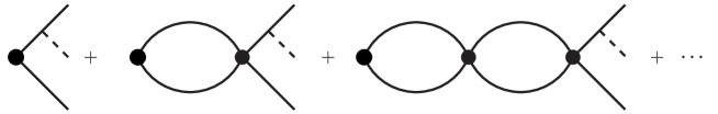
Figure 11: Diagrams at order $g$ for the vacuum–to–$D_{1}D_{2}\phi$ matrix element of the operator $\lambda_{0}D_{1}^{\dagger}D_{2}^{\dagger}$.

We first calculate the rate for $A\to B+D_{1}D_{1}\phi$ to order $g^{2}$ using ordinary perturbation theory. At order $g$, the operator matrix element in Eq. (28b) is given by the series of Feynman diagrams in Fig. 11 summed over the two permutations of the external $D_{1}$ lines. The sum of the geometric series of diagrams is $\mathcal{A}_{0}(M)/(-\lambda_{0})$ multiplied by the first diagram in the series. According to the Optical Theorem, the square of the first diagram integrated over the 3-body phase space for $D_{1}D_{1}\phi$ is given by the sum of the 3-body cuts through the Feynman diagrams for $L_{2}(E)$ in Fig. 8. If $M<M_{1+2}$, the sum of the 3-body cuts gives the imaginary part of $L_{2}(E)$. Thus the square of the T-matrix element in Eq. (28b) integrated over the 3-body phase space of $D_{1}D_{1}\phi$ is

$$\frac{1}{2}\int\frac{d^{3}p_{1}}{(2\pi)^{3}2E_{1}}\frac{d^{3}p_{2}}{(2\pi)^{3}2E_{2}}\frac{d^{3}k}{(2\pi)^{3}2\omega}(2\pi)^{4}\delta(P-p_{1}-p_{2}-k)\left|{\cal T}[A\to B+D_{1}D_{1}\phi]\right|^{2}$$

$$\hskip 199.16928pt=|{\cal C}_{A}^{B,12}|^{2}|\mathcal{A}_{0}(M)|^{2}(-2)\,{\rm Im}\,L_{2}(M),$$ (83)

where $p_{1}$, $p_{2}$, and $k$ are 4-momenta for $D_{1}$, $D_{1}$, and $\phi$, respectively, and $P^{2}=M^{2}$. If $A$ consists of a single particle, the invariant mass distribution for $A\to B+D_{1}D_{1}\phi$ at order $g^{2}$ can be expressed as

$$\frac{d\Gamma}{dM}[A\to B+D_{1}D_{1}\phi] = \Gamma_{A}^{B}\,\frac{M_{12}}{2\pi}\left|\mathcal{A}_{0}(M)\right|^{2}(-2)\,{\rm Im}\,L_{2}(M),$$ (84)

where $\Gamma_{A}^{B}$ is the short-distance factor defined in Eq. (49) and we have replaced a multiplicative factor of $M$ by $M_{1+2}$.

If there is a short-distance process $A\to B+D_{1}D_{1}\phi$, then the process $A\to B+D_{1}D_{2}$ is also allowed. The invariant mass distribution for $A\to B+D_{1}D_{2}$ at order $g^{0}$ is given by the expression on the right side of Eq. (84) with ${\rm Im}\,L_{2}(M)$ replaced by ${\rm Im}\,L_{0}(M)$. The threshold for this process is $M>M_{1+2}$. Since $D_{2}$ ultimately decays into $D_{1}\phi$, a decay into $D_{1}D_{2}$ can also be regarded as a contribution to the inclusive decay into $D_{1}D_{1}\phi$.

The result in Eq. (84) is an order $g^{2}$ correction to the inclusive invariant mass distribution for $D_{1}D_{1}\phi$. It is nonzero for all $M>2M_{1}+m$. For $M>M_{1+2}$, there are additional corrections of order $g^{2}$ that can be obtained by replacing any of the one-loop subdiagrams in Fig. 11 by one of the two-loop diagrams for $L_{2}(E)$ in Fig. 8. Nonperturbative renormalization of the coupling constant $\lambda_{0}$ then requires that a geometric series of these corrections be summed to all orders. The net effect is to replace $\mathcal{A}_{0}(M)$ in Eq. (84) by $\mathcal{A}_{2}(M)$. Thus the complete result for the inclusive invariant mass distribution for $D_{1}D_{1}\phi$ through order $g^{2}$ is

$$\frac{d\Gamma}{dM}[A\to B+D_{1}D_{1}\phi] = \Gamma_{A}^{B}\,\frac{M_{12}}{2\pi}\left|\mathcal{A}_{2}(M)\right|^{2}(-2)\,{\rm Im}\,[L_{0}(M)+L_{2}(M)],$$ (85)

where the functions $\mathcal{A}_{2}(M)$, $L_{0}(M)$, and $L_{2}(M)$ are given in Eqs. (65), (31), and (59). Note that taking the imaginary parts of $L_{0}(M)$ and $L_{2}(M)$ eliminates the additive ultraviolet-divergent terms. A more compact expression for the distribution in Eq. (85) is

$$\frac{d\Gamma}{dM}[A\to B+D_{1}D_{1}\phi] = \Gamma_{A}^{B}\,\frac{M_{12}}{\pi}\,{\rm Im}\,\mathcal{A}_{2}(M).$$ (86)

The inclusive invariant mass distribution in Eq. (85) when calculated using ordinary perturbation theory has unphysical behavior at the threshold $M=M_{1+2}$. The factor $|\mathcal{A}_{2}(M)|^{2}$ has a zero at $M=M_{1+2}$ and a sharp peak just above that threshold as illustrated in Fig. 9. The term $-2\,{\rm Im}L_{2}(M)$ also has unphysical behavior at this threshold. The imaginary part of $L_{2}(E)$ in the region $2M_{1}+m<E<M_{1+2}$ is given by the sum of Eqs. (115) and (123). The resulting expression for $-2\,{\rm Im}\,L_{2}(E)$ is

$$-2\,{\rm Im}\,L_{2}(E)=\frac{g^{2}M_{12}^{2}m_{1}}{\pi^{2}}\left[2\int_{0}^{z_{0}}\frac{dz}{z^{2}}\left(\frac{t^{3}(z)}{1-t(z)}\right)^{1/2}+\left(\frac{m_{1}}{M_{12}}\right)^{1/2}\,\frac{(\kappa_{1}-\kappa(E))^{2}}{2\kappa_{1}\kappa(E)}\right],$$ (87)

where the upper limit $z_{0}$ of the integral is

$$z_{0}=\frac{(m_{1}/M_{12})(\kappa_{1}^{2}-\kappa(E)^{2})}{(m_{1}/M_{12})(\kappa_{1}^{2}-\kappa(E)^{2})+\kappa(E)^{2}}.$$ (88)

The function in Eq. (87) diverges like $1/\kappa(E)$ as $E\to M_{1+2}$. As a consequence, near the $D_{1}D_{2}$ threshold, corrections of higher order in $g^{2}$ that come from the $D_{2}$ self energy are not suppressed. This is the same problem that prompted us to introduce the complex mass scheme in Section IV.1.

We next consider the inclusive rate for $A\to B+D_{1}D_{1}\phi$ in the complex mass scheme. At LO in the complex mass scheme, the invariant mass distribution for $D_{1}D_{1}\phi$ can be obtained from Eq. (86) by replacing $\mathcal{A}_{2}(M)$ by $\mathcal{A}_{0}(M)$ in Eq. (36). This can be written more explicitly as

$$\frac{d\Gamma}{dM}[A\to B+D_{1}D_{1}\phi] = \Gamma_{A}^{B}\,\frac{-2\,{\rm Im}\,\gamma(M)}{|\gamma(M)-{\rm Re}\,\gamma_{X}|^{2}},$$ (89)

where $\gamma(E)$ and $\gamma_{X}$ are defined in Eqs. (37) and (38). This expression has a nonzero imaginary part at all energies $E$, even below the $D_{1}D_{1}\phi$ theshold. For $E<2M_{1}+m$, the imaginary part is small and it is cancelled by higher orders in the complex mass scheme. At NLO in the complex mass scheme, the invariant mass distribution for $D_{1}D_{1}\phi$ is obtained from Eq. (86) by using the expression for $\mathcal{A}_{2}(M)$ in Eq. (70).

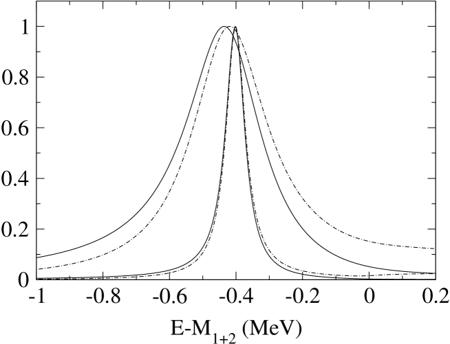
Figure 12: Line shapes of the $X$ resonance at NLO in the complex mass scheme. The solid lines are for a short-distance decay channel ($|\mathcal{A}_{2}(E)|^{2}$ using $\mathcal{A}_{2}(E)$ in Eq. (70)). The dash-dotted lines are for the $D_{1}D_{1}\phi$ channel (${\rm Im}\,\mathcal{A}_{2}(E)$ using $\mathcal{A}_{2}(E)$ in Eq. (70)). The line shapes are shown for $\kappa_{X}=27.8$ MeV and for both $\Gamma_{2}=0.07$ MeV (narrower resonances) and $\Gamma_{2}=0.28$ MeV (wider resonances). The line shapes are normalized so their maximum values are 1.

In Fig. 12, we compare the line shape of $X$ in the $D_{1}D_{1}\phi$ channel, which is proportional to ${\rm Im}\,\mathcal{A}_{2}(E)$, with the line shape of $X$ in a short-distance decay channel, which is proportional to $|\mathcal{A}_{2}(E)|^{2}$. They are shown for two values of the coupling constant $g$ that correspond to the width of $D_{2}$ being $\Gamma_{2}=0.07$ MeV and $0.28$ MeV. The curves are normalized so their maximum values are 1. The line shapes have the same qualitative behavior. The line shape for $D_{1}D_{1}\phi$ is shifted towards higher energy by an amount that decreases as $g$ decreases.

The Belle Collaboration has observed an enhancement in the production of $D^{0}\bar{D}^{0}\pi^{0}$ near threshold in the decay $B\to K+D^{0}\bar{D}^{0}\pi^{0}$ Gokhroo:2006bt . The enhancement peaks at the invariant mass $3875.2^{+1.1}_{-1.9}$ MeV, where we have combined the errors in quadrature. If we use the recent precision measurement of the $D^{0}$ mass by the CLEO Collaboration Cawlfield:2007dw , the peak is above the $D^{*0}\bar{D}^{0}$ threshold by $3.4^{+1.2}_{-1.9}$ MeV. In contrast, the peak observed in the short-distance decay channel $J/\psi\,\pi^{+}\pi^{-}$ is below the $D^{*0}\bar{D}^{0}$ threshold by $0.6\pm 0.6$ MeV. The difference is $4.0^{+1.3}_{-2.0}$ MeV, which differs from 0 by two standard deviations. Part of the discrepancy may be due to a shift in the invariant mass distribution analogous to the one illustrated in Fig. 12.

IV.7 Decay of $\bm{X}$ into $\bm{D_{1}D_{1}\phi}$

The width $\Gamma_{X}$ of the $X$ resonance was defined in Eq. (11) in terms of the energy $E_{\rm pole}$ of the pole in the $X$ propagator: $\Gamma_{X}=-2\,{\rm Im}\,E_{\rm pole}$. At LO in the complex mass scheme, $\Gamma_{X}$ is simply $\Gamma_{2}$. At NLO in the complex mass scheme, $\Gamma_{X}$ is obtained by solving Eq. (75) for $E_{\rm pole}$. If the width of the $X$ resonance is sufficiently small, its width can also be interpreted as its decay rate. A direct calculation of that decay rate will give a result that is closely related to but not identical to $\Gamma_{X}$. We will denote the result of the direct calculation of the inclusive decay rate by $\Gamma[X\to D_{1}D_{1}\phi]$.

We can use the Optical Theorem to calculate the inclusive decay rate for $X\to D_{1}D_{1}\phi$:

$$\Gamma[X\to D_{1}D_{1}\phi]=\frac{1}{M_{X}}\,{\rm Im}\,{\cal T}[X\to X].$$ (90)

The forward T-matrix element for $X\to X$ can be defined using the LSZ formalism and it is given in Eq. (27). At NLO in the complex mass scheme, the normalization constant $Z_{X}$ and the propagator $\Delta_{X}(E,0)$ are given in Eqs. (76) and (73). The resulting expression for the decay rate of $X$ in Eq. (90) is

$$\Gamma[X\to D_{1}D_{1}\phi]=-2\,{\rm Im}\frac{Z_{X}{\cal A}_{2}^{-1}(M_{X})}{\lambda_{0}[L_{0}(M_{X})+L_{2}(M_{X})]}.$$ (91)

We have used Eq. (64) to express this in a form with a factor of ${\cal A}_{2}^{-1}(M_{X})$, because ${\cal A}_{2}(E)$ does not depend on the ultraviolet cutoff $\Lambda$. The decay rate in Eq. (91) depends on $\Lambda$ through the bare coupling constant $\lambda_{0}$ and through the ultraviolet-divergent additive constants in $L_{0}(M_{X})$ and $L_{2}(M_{X})$. From the renormalized expression for ${\cal A}_{2}(E)$ in Eq. (64), we can see that the divergent terms in $L_{0}(E)+L_{2}(E)$ must be cancelled by $1/\lambda_{0}$ as $\Lambda\to\infty$. The leading divergence is a linear divergence in $L_{0}(M_{1+2})$ that is linear in $\Lambda$. Thus $1/\lambda_{0}$ must include a cancelling linear divergence. This implies that $\lambda_{0}[L_{0}(E)+L_{2}(E)]$ must approach 1 as $\Lambda\to\infty$. Upon taking the limit $\Lambda\to\infty$, Eq. (91) reduces to

$$\Gamma[X\to D_{1}D_{1}\phi]=-2\,{\rm Im}\left(Z_{X}\mathcal{A}_{2}^{-1}(M_{X})\right).$$ (92)

An explicit expression for the inclusive decay rate of $X$ can be obtained from Eq. (92) by inserting the renormalized expression for ${\cal A}_{2}(E)$ in Eq. (70):

$$\Gamma[X\to D_{1}D_{1}\phi]=\frac{M_{12}}{2\pi}\,(-2)\,{\rm Im}\left[Z_{X}\big{(}\gamma(M_{X})+F_{\rm cms}(\gamma(M_{X}))-{\rm Re}[\gamma_{X}+F_{\rm cms}(\gamma_{X})]\big{)}\right],$$

(93)

where $Z_{X}$, $\gamma(E)$, $\gamma_{X}$, and $F_{\rm cms}(\gamma)$ are given in Eqs. (76), (37), (38), and (71). If we treat $\Gamma_{2}$ as order $g^{2}$, the decay rate in Eq. (93) reduces at order $g^{2}$ to the corresponding result for the width $\Gamma_{X}$ in Eq. (78b).

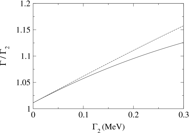
Figure 13: The width $\Gamma_{X}$ of the $X$ resonance (solid line) and the decay rate $\Gamma[X\to D_{1}D_{1}\phi]$ (dashed line) at NLO in the complex mass scheme as functions of $\Gamma_{2}$. The vertical axis is in units of $\Gamma_{2}$. The intercept on the vertical axis is approximately $1.011$.

In Fig. 13, we compare the width $\Gamma_{X}$ obtained by solving Eq. (75) and the decay rate $\Gamma[X\to D_{1}D_{1}\phi]$ in Eq. (93) as functions of $\Gamma_{2}$. They agree for small $\Gamma_{2}$, because the difference between $\Gamma_{X}$ and $\Gamma[X\to D_{1}D_{1}\phi]$ is of order $g^{4}$. They differ by less than 1% if $\Gamma_{2}<0.16$ MeV.

V Summary

We have examined the effects of a weakly-bound hadronic molecule on a nearby 3-body threshold, where the three bodies consist of a primary constituent of the molecule and the decay products of the other constituent. We studied these effects in the simplest possible model: the scalar meson model, with spin-0 constituents $D_{1}$, $D_{2}$, and $\phi$ and momentum-independent interactions. The primary constitutents of the molecule $X$ are $D_{1}D_{2}$ and the 3-body threshold is that for $D_{1}D_{1}\phi$. The $D_{1}D_{2}$ contact interaction with coupling constant $\lambda_{0}$ was treated nonperturbatively. The $D_{2}-D_{1}\phi$ interaction with coupling constant $g$ was treated perturbatively. Several observables were calculated to all orders in $\lambda_{0}$ and to next-to-leading order in $g$. Both ultraviolet problems and infrared problems were encountered in these calculations.

We found that at next-to-leading order in $g$, the ultraviolet divergences can be removed by a perturbative renormalization of the $D_{2}$ mass, a nonperturbative renormalization of $\lambda_{0}$, and a nonperturbative renormalization of short-distance coefficients in the operator product expansion. The nonperturbative renormalizations required the summing of a geometric series of order-$g^{2}$ subdiagrams to all orders. The subdiagrams represent order-$g^{2}$ contributions to the amplitude for the propagation of $D_{1}D_{2}$ between contact interactions. Thus the renormalized amplitudes at next-to-leading order include all terms of order $g^{2}$ together with subsets of terms from all higher orders in $g$.

We found that the next-to-leading order amplitudes suffer from an infrared problem at the $D_{1}D_{2}$ threshold. The problem is illustrated dramatically in Fig. 9, which shows the line shape $|\mathcal{A}(E)|^{2}$ in a short-distance decay channel as a function of the energy $E$. The pathological behavior at $E=M_{1+2}$ arises because the $D_{2}-D_{1}\phi$ interaction shifts the $D_{1}D_{2}$ threshold from the real value $M_{1+2}$ to the complex value $M_{1+2}-i\Gamma_{2}/2$. Since $\Gamma_{2}$ is of order $g^{2}$, a strict expansion in powers of $g$ leads to singularities at $E=M_{1+2}$. One possible solution to this problem is to sum the geometric series of self-energy corrections to the $D_{2}$ propagator to all orders, but this leads to very complicated loop integrals. A simpler solution is to use the complex mass scheme, in which the width $\Gamma_{2}$ is included in the Feynman rule for the $D_{2}$ propagator and its effects are systematically compensated at higher orders in $g$ through counterterms. This partial resummation of the $D_{2}$ propagator corrections leads to smooth behavior of the line shape $|\mathcal{A}(E)|^{2}$ at the $D_{1}D_{2}$ threshold as illustrated in Fig. 10. Having solved the infrared problems, we calculated several observables to NLO in the complex mass scheme. They include the line shapes of the $X$ resonance in both a short-distance decay channel and in the $D_{1}D_{1}\phi$ channel.

The $X(3872)$ is a weakly-bound hadronic molecule whose primary constitutents are a superposition of charm mesons: $D^{*0}\bar{D}^{0}+D^{0}\bar{D}^{*0}$. Its mass is near the 3-body thresholds for $D^{0}\bar{D}^{0}\pi^{0}$, $D^{0}D^{-}\pi^{+}$, and $D^{+}\bar{D}^{0}\pi^{-}$. The methods we applied to the scalar meson model can be extended straightforwardly to this multichannel problem. A conventional perturbation expansion in the $D^{*}-D\pi$ coupling constant will have infrared problems at the $D^{*0}\bar{D}^{0}$ threshold which are associated with the decay $D^{*0}\to D^{0}\pi^{0}$. These infrared problems can be avoided by using the complex mass scheme. The ultraviolet problems can be expected to be more severe in this system, because the $D^{*}-D\pi$ interaction is proportional to the 3-momentum of the pion. Thus renormalization may not be as simple as in the scalar meson model. If the renormalization problem can be solved, it will be straightforward to calculate observables to NLO in the complex mass scheme. One of the most interesting applications will be to predict the difference between the line shapes of the $X(3872)$ resonance in a short-distance decay channel, such as $J/\psi\,\pi^{+}\pi^{-}$, and in the $D^{0}\bar{D}^{0}\pi^{0}$ channel.

Appendix A Loop Integrals

In this appendix, we calculate the loop integrals that appear at order $g^{0}$ and at order $g^{2}$ in the scalar meson model.

A.1 Dimensional regularization

Many of the loop integrals we need to evaluate are ultraviolet divergent. They can be regularized by using dimensional regularization of the integrals over the 3-momenta. We analytically continue the 3-dimensional integrals to $3-2\epsilon$ dimensions using the prescription

$$\int_{\vec{k}}\equiv\lim_{\epsilon\to 0}~{}(4\pi)^{-\epsilon}\left(\mbox{$\frac{3}{2}$}\right)_{-\epsilon}\mu^{2\epsilon}\int\!\frac{d^{3-2\epsilon}k}{(2\pi)^{3-2\epsilon}},$$ (94)

where $\mu$ is the renormalization scale and $(z)_{a}$ is the Pochhammer symbol:

$$\left(z\right)_{a}=\frac{\Gamma(z+a)}{\Gamma(z)}.$$ (95)

The function of $\epsilon$ in the prefactor is designed to simplify the analytic expressions for dimensionally regularized integrals by cancelling the effects of the analytic continuation of angular integrals. Thus the integral of a scalar function of $\vec{k}$ is

$$\int_{\vec{k}}f(|\vec{k}\,|)\equiv\lim_{\epsilon\to 0}~{}\frac{1}{2\pi^{2}}\mu^{2\epsilon}\int_{0}^{\infty}\!dk~{}k^{2-2\epsilon}f(k).$$ (96)

Loop integrals are evaluated by first inserting the appropriate nonrelativistic propagators:

$$\Delta_{i}(p_{0},p) = \frac{i}{p_{0}-M_{i}-p^{2}/(2M_{i})+i\varepsilon},$$ (97)

where $i=1,2,\phi$ and $M_{\phi}=m$. Integrals over the loop energy are then evaluated using the residue theorem. After using the Feynman parameter trick to combine denominators, the dimensionally regularized integrals over the 3-momenta can be evaluated. The final steps are the evaluation of the Feynman parameter integrals and the analytic continuation to $\epsilon=0$. It will be convenient to express the results in terms of the variables

$$\kappa = \left[-2M_{12}(E-M_{1+2})-i\varepsilon\right]^{1/2},$$ (98a)

$$\kappa_{1} = \left[2M_{12}(M_{2-1}-m)\right]^{1/2}.$$ (98b)

A.2 Self-energy of $\bm{D_{2}}$

The one-loop diagram for the self-energy $\Sigma(p_{0},p)$ of $D_{2}$ is shown in Fig. 2(a). The expression for the diagram is

$$\Sigma_{2a}(p_{0},p)=-ig^{2}\int\!\!\frac{d^{4}q}{(2\pi)^{4}}\,\Delta_{1}(q_{0},q)\,\Delta_{\phi}(p_{0}-q_{0},|\vec{p}-\vec{q}\,|).$$ (99)

The residue theorem can be used to evaluate the energy integral:

$$\Sigma_{2a}(p_{0},p)=g^{2}\int_{\vec{q}}\frac{1}{p_{0}-M_{1}-m-q^{2}/(2M_{1})-(\vec{p}-\vec{q}\,)^{2}/(2m)+i\varepsilon}.$$ (100)

If we implement dimensional regularization using the prescription in Eq. (94), the analytic result is

$$\Sigma_{2a}(p_{0},p)=\frac{g^{2}m_{1}\mu^{2\epsilon}}{2\pi\cos(\pi\epsilon)}\left(-2m_{1}\bigg{[}p_{0}-M_{1}-m-\frac{p^{2}}{2(M_{1}+m)}\bigg{]}-i\varepsilon\right)^{\frac{1}{2}-\epsilon}.$$ (101)

The self-energy in dimensional regularization is given by the analytic continuation of Eq. (101) to $\epsilon=0$:

$$\Sigma_{2a}(p_{0},p)=\frac{g^{2}m_{1}}{2\pi}\left(-2m_{1}\bigg{[}p_{0}-M_{1}-m-\frac{p^{2}}{2(M_{1}+m)}\bigg{]}-i\varepsilon\right)^{\frac{1}{2}}.$$ (102)

The momentum integral in Eq. (100) has a linear ultraviolet divergence that is set to zero by dimensional regularization. The self-energy in a general regularization scheme is given in Eq. (16). The linear ultraviolet divergence is contained in the extra term $\Sigma_{2a}(M_{1}+m,0)$, which is real valued.

A.3 Propagation between contact interactions at leading order

The amplitude for the propagation of $D_{1}D_{2}$ between contact interactions is given at order $g^{0}$ by the one-loop diagram in Fig. 4. In the center-of-momentum frame where the 4-momentum is $(E,0)$, this amplitude is

$$iL_{0}(E)=\int\frac{d^{4}q}{(2\pi)^{4}}\,\Delta_{2}(q_{0},q)\,\Delta_{1}(E-q_{0},q).$$ (103)

The residue theorem can be used to evaluate the energy integral:

$$L_{0}(E)=\int_{\vec{q}}\frac{1}{(E-M_{1+2})-q^{2}/2M_{12}+i\varepsilon}.$$ (104)

If we implement dimensional regularization using the prescription in Eq. (94), the analytic result is

$$L_{0}(E)=\frac{M_{12}\mu^{2\epsilon}}{2\pi\cos(\epsilon\pi)}\kappa^{1-2\epsilon},$$ (105)

where $\kappa$ is defined in Eq. (98a). The amplitude in dimensional regularization is given by analytic continuation to $\epsilon=0$:

$$L_{0}(E)=\frac{M_{12}}{2\pi}\kappa.$$ (106)

The momentum integral in Eq. (104) has a linear ultraviolet divergence that is set to zero by dimensional regularization. The amplitude in a general regularization scheme is given in Eq. (31). The linear ultraviolet divergence is contained in the extra term $L_{0}(M_{1+2})$, which is real valued.

A.4 Propagation between contact interactions at next-to-leading order

The amplitude for the propagation of $D_{1}D_{2}$ between contact interactions has contribution of order $g^{2}$ from the two-loop diagrams in Fig. 8. In the center-of-momentum frame where the 4-momentum is $(E,\vec{0})$, the order-$g^{2}$ amplitude $iL_{2}(E)$ is a function of $E$ only. We proceed to calculate the contributions from each of the three diagrams.

A.4.1 Correction from $\bm{\phi}$ exchange

The contribution to the amplitude $iL_{2}(E)$ from the two-loop diagram in Fig. 8(a) in which $\phi$ is exchanged between the $D_{1}$ and $D_{2}$ is

$$iL_{2a}(E) = -g^{2}\int\frac{d^{4}k}{(2\pi)^{4}}\int\frac{d^{4}q}{(2\pi)^{4}}\,\Delta_{2}(k_{0},k)\,\Delta_{1}(E-k_{0},k)$$ (107)

$$\hskip 28.45274pt\times\Delta_{2}(q_{0},q)\,\Delta_{1}(E-q_{0},q)\,\Delta_{\phi}(k_{0}+q_{0}-E,|\vec{k}+\vec{q}\,|).$$

The integrals over the loop energies $k_{0}$ and $q_{0}$ can be evaluated by closing the contours in the upper half-planes. After introducing Feynman parameters and evaluating the integrals over the loop momenta, the amplitude reduces to

$$L_{2a}(E) = -\frac{g^{2}M_{12}^{2}m_{1}}{16\pi^{3}}\,\frac{(1-2\epsilon)^{2}\left(\frac{1}{2}\right)^{2}_{-\epsilon}\left(1\right)_{\epsilon}}{\epsilon}\mu^{4\epsilon}$$ (108)

$$\times\int_{0}^{1}\!dx\int_{0}^{1-x}\!dy\,\left[(1-x)(1-y)-(m_{1}/m)^{2}(1-x-y)^{2}\right]^{-3/2+\epsilon}$$

$$\hskip 56.9055pt\times\left[(x+y)\kappa^{2}+(1-x-y)(m_{1}/M_{12})(\kappa^{2}-\kappa_{1}^{2})\right]^{-2\epsilon},$$

where $\kappa$ and $\kappa_{1}$ are defined in Eqs. (98). One of the Feynman parameter integrals can be evaluated analytically by changing variables to $z=x+y$ and $w=(x-y)/(x+y)$. The integral over $w$ gives a hypergeometric function:

$$L_{2a}(E) = -\frac{g^{2}M_{12}^{2}m_{1}}{2\pi^{3}}\,\frac{(1-2\epsilon)^{2}\left(\frac{1}{2}\right)^{2}_{-\epsilon}\left(1\right)_{\epsilon}2^{-2\epsilon}}{\epsilon}\mu^{4\epsilon}\int_{0}^{1}\!dz\,z^{-2+2\epsilon}\,t(z)^{3/2-\epsilon}\,$$ (109)

$$\hskip 28.45274pt\times{}_{2}F_{1}(\mbox{$\frac{3}{2}-\epsilon$},\mbox{$\frac{1}{2}$},\mbox{$\frac{3}{2}$};t(z))\left[z\kappa^{2}+(1-z)(m_{1}/M_{12})(\kappa^{2}-\kappa_{1}^{2})\right]^{-2\epsilon},$$

where $t(z)$ is the rational function of $z$ given in Eq. (62). The pole at $\epsilon=0$ in Eq. (109) is a logarithmic ultraviolet divergence.

The amplitude $L_{2a}(E)$ in dimensional regularization is defined by the Laurent expansion of the expression in Eq. (109) to order $\epsilon^{0}$. The expansion in powers of $\epsilon$ is facilitated by using a transformation formula to replace the hypergeometric function in Eq. (109) by one of the form ${}_{2}F_{1}(1,\epsilon,\frac{3}{2};t)$:

$${}_{2}F_{1}(\mbox{$\frac{3}{2}-\epsilon$},\mbox{$\frac{1}{2}$},\mbox{$\frac{3}{2}$};t)={}_{2}F_{1}(1,\epsilon,\mbox{$\frac{3}{2}$};t)(1-t)^{-1/2+\epsilon}.$$ (110)

The expansion of ${}_{2}F_{1}(1,\epsilon,\frac{3}{2};t)$ to order $\epsilon$ is simple:

$${}_{2}F_{1}(1,\epsilon,\mbox{$\frac{3}{2}$};t)=1+\mbox{$\frac{2}{3}$}\epsilon\,t\;{}_{2}F_{1}(1,1,\mbox{$\frac{5}{2}$};t)+\ldots.$$ (111)

Expanding the amplitude $L_{2a}(E)$ in Eq. (109) to 0^th order in $\epsilon$, it reduces to

$$L_{2a}(E) = -\frac{g^{2}M_{12}^{2}m}{2\pi^{3}}\,\Bigg{(}\frac{1}{2}\arcsin\frac{m_{1}}{m}\left(\frac{1}{\epsilon}-4+\gamma+2\ln 2\right)$$ (112)

$$\hskip 28.45274pt+\frac{m_{1}}{m}\int_{0}^{1}\frac{dz}{z^{2}}\,\left(\frac{t^{3}(z)}{1-t(z)}\right)^{1/2}\bigg{[}\ln\frac{z^{2}[1-t(z)]}{t(z)}+\frac{2t(z)}{3}\,{}_{2}F_{1}\left(1,1,\mbox{$\frac{5}{2}$};t(z)\right)$$

$$\hskip 142.26378pt-2\ln\frac{z\kappa^{2}+(1-z)(m_{1}/M_{12})(\kappa^{2}-\kappa_{1}^{2})}{\mu^{2}}\bigg{]}\Bigg{)}.$$

We have used the integral

$$\int_{0}^{1}\frac{dz}{z^{2}}\,\left(\frac{t^{3}(z)}{1-t(z)}\right)^{1/2}=\frac{m}{2m_{1}}\arcsin\frac{m_{1}}{m}.$$ (113)

This can be evaluated by changing variables to $w=z/[z+2r(1-z)]$. Most of the terms in Eq. (112) are independent of $E$. The expression can be simplified by expressing it in the form

$$L_{2a}(E)=L_{2a}(2M_{1}+m) + \frac{g^{2}M_{12}^{2}m_{1}}{\pi^{3}}\int_{0}^{1}\frac{dz}{z^{2}}\left(\frac{t^{3}(z)}{1-t(z)}\right)^{1/2}$$ (114)

$$\hskip 56.9055pt\times\ln\frac{z\kappa^{2}+(1-z)(m_{1}/M_{12})(\kappa^{2}-\kappa_{1}^{2})}{z\kappa_{1}^{2}}.$$

The amplitude $L_{2a}(2M_{1}+m)$ at the $D_{1}D_{1}\phi$ threshold is real-valued and includes the logarithmic divergence. The amplitude $L_{2a}(E)$ has an imaginary part for $E>2M_{1}+m$. For energies in the range $2M_{1}+m<E<M_{1+2}$, the imaginary part is

$${\rm Im}\,L_{2a}(E) = -\frac{g^{2}M_{12}^{2}m_{1}}{\pi^{2}}\int_{0}^{z_{0}}\frac{dz}{z^{2}}\left(\frac{t^{3}(z)}{1-t(z)}\right)^{1/2},$$ (115)

where the upper limit $z_{0}$ of the integral is

$$z_{0}=\frac{(m_{1}/M_{12})(\kappa_{1}^{2}-\kappa^{2})}{(m_{1}/M_{12})(\kappa_{1}^{2}-\kappa^{2})+\kappa^{2}}.$$ (116)

The first few terms in the Laurent expansion of $L_{2a}(E)$ in powers of $\kappa$ are

$$L_{2a}(E)\approx L_{2a}(2M_{1}+m) + \frac{g^{2}M_{12}^{2}m_{1}}{2\pi^{3}}\Bigg{[}2\int_{0}^{1}\frac{dz}{z^{2}}\left(\frac{t^{3}(z)}{1-t(z)}\right)^{1/2}\ln\frac{(1-z)m_{1}}{zM_{12}}$$ (117)

$$\hskip 42.67912pt-i\pi\frac{m}{m_{1}}\arcsin\frac{m_{1}}{m}+2\pi i\left(\frac{M_{12}}{m_{1}}\right)^{1/2}\frac{\kappa}{\kappa_{1}}\Bigg{]}.$$

A.4.2 Correction from $\bm{D_{2}}$ self-energy

The contribution to $iL_{2}(E)$ from the two-loop diagram in Fig. 8(b) with a self-energy correction to the $D_{2}$ line is

$$iL_{2b}(E) = -i\int\frac{d^{4}k}{(2\pi)^{4}}\,\Delta_{2}(k_{0},k)^{2}\,\Delta_{1}(E-k_{0},k)\,\Sigma_{2a}(k_{0},k),$$ (118)

where $\Sigma_{2a}(k_{0},k)$ is the contribution to the $D_{2}$ self-energy from the one-loop diagram in Fig. 2(a). The analytic result for $\Sigma_{2a}(k_{0},k)$ in dimensional regularization is given in Eq. (101). Since $\Sigma_{2a}(k_{0},k)$ has a branch cut for $k_{0}$ in the lower half-plane, it is convenient to close the $k_{0}$ contour in the upper half-plane. After introducing Feynman parameters, the integral over $\vec{k}$ can be evaluated. If we implement dimensional regularization using the prescription in Eq. (94), the result is

$$L_{2b}(E) = -\frac{g^{2}M_{12}^{2}m_{1}}{16\pi^{3}}\,\left(\frac{m_{1}}{M_{11}}\right)^{1/2-\epsilon}\,\frac{(1-2\epsilon)^{2}(1)_{2\epsilon}}{(\frac{1}{2})_{\epsilon}^{2}\cos^{2}(\pi\epsilon)\epsilon}\mu^{4\epsilon}$$ (119)

$$\times\int_{0}^{1}\!dx\,x(1-x)^{-3/2+\epsilon}\left[x\kappa^{2}+(1-x)(M_{11}/M_{12})(\kappa^{2}-\kappa_{1}^{2})\right]^{-2\epsilon},$$

where $\kappa$ and $\kappa_{1}$ are defined in Eqs. (98) and $M_{11}$ is given by

$$M_{11} = \frac{M_{1}(M_{1}+m)}{2M_{1}+m}.$$ (120)

The pole at $\epsilon=0$ in Eq. (119) is a logarithmic ultraviolet divergence.

The amplitude $L_{2b}(E)$ in dimensional regularization is defined by the Laurent expansion of the expression in Eq. (119) to order $\epsilon^{0}$. Expanding to 0^th order in $\epsilon$, the expression reduces to

$$L_{2b}(E) = \frac{g^{2}M_{12}^{2}m_{1}}{4\pi^{3}}\left(\frac{m_{1}}{M_{11}}\right)^{1/2}\,\Bigg{[}\frac{1}{\epsilon}-4+4\ln 2-\ln\frac{m_{1}}{M_{11}}-2\ln\frac{\kappa^{2}}{\mu^{2}}$$ (121)

$$+\mbox{$\frac{1}{2}$}\int_{0}^{1}\!dx\,x(1-x)^{-3/2}\ln\frac{x\kappa^{2}+(1-x)(M_{11}/M_{12})(\kappa^{2}-\kappa_{1}^{2})}{\kappa^{2}}\Bigg{]}.$$

The integral over $x$ can be evaluated analytically. We can simplify the expression by replacing $M_{11}/M_{12}$ by 1, because the difference is suppressed by a factor of $\kappa_{1}^{2}/M_{2}^{2}$. Most of the terms in Eq. (121) are independent of $E$. The expression can be simplified by expressing it in the form

$$L_{2b}(E)=L_{2b}(2M_{1}+m)-\frac{g^{2}M_{12}^{2}m_{1}}{2\pi^{3}}\left(\frac{m_{1}}{M_{12}}\right)^{1/2}\,\left(2\ln\frac{\kappa+\kappa_{1}}{2\kappa_{1}}+\frac{(\kappa-\kappa_{1})^{2}}{2\kappa\kappa_{1}}\ln\frac{\kappa+\kappa_{1}}{\kappa-\kappa_{1}}\right).$$

(122)

The amplitude $L_{2b}(2M_{1}+m)$ at the $D_{1}D_{1}\phi$ threshold is real-valued and includes the logarithmic divergence. The amplitude $L_{2b}(E)$ has an imaginary part for $E>2M_{1}+m$. For energies in the range $2M_{1}+m<E<M_{1+2}$, the imaginary part of $L_{2b}(E)$ is

$${\rm Im}\,L_{2b}(E) = -\frac{g^{2}M_{12}^{2}m_{1}}{4\pi^{2}}\left(\frac{m_{1}}{M_{12}}\right)^{1/2}\,\frac{(\kappa_{1}-\kappa)^{2}}{\kappa\kappa_{1}}.$$ (123)

Note that this diverges at the $D_{1}D_{2}$ threshold $\kappa=0$. The first few terms in the Laurent expansion of $L_{2a}(E)$ in powers of $\kappa$ are

$$L_{2b}(E)\approx L_{2b}(2M_{1}+m)-\frac{g^{2}M_{12}^{2}m_{1}}{2\pi^{3}}\left(\frac{m_{1}}{M_{12}}\right)^{1/2}\left[1-2\ln 2+i\pi\left(\frac{\kappa_{1}}{2\kappa}-1+\frac{\kappa}{2\kappa_{1}}\right)\right].$$

(124)

A.4.3 Correction from counterterms

In a general regularization scheme, the one-loop self-energy subdiagram $\Sigma_{2a}(k_{0},k)$ in Eq. (118) has a linear ultraviolet divergence, which is included in the term $\Sigma_{2a}(M_{1}+m,0)$ in Eq. (16). The resulting divergence in $L_{2b}(E)$ is cancelled by the one-loop diagram with a $D_{2}$ mass counterterm in Fig. 8(c). The counterterm vertex is $-i\delta M$, with $\delta M=\Sigma_{2a}(M_{1}+m,0)$.

In the complex mass scheme, the $D_{2}$ propagator counterterm has the more complicated form given in Eq. (23). With this counterterm, the contribution to $L_{2}(E)$ of order $g^{2}$ from the one-loop diagram in Fig. 8(c) is

$$iL_{2c}(E) = -i\int\frac{d^{4}k}{(2\pi)^{4}}\Delta_{1}(E-k_{0},k)\Delta_{2}(k_{0},k)^{2}\Big{(}(\delta M+i\Gamma_{2}/2)$$ (125)

$$\hskip 142.26378pt+(Z_{2}^{-1}-1)[k_{0}-M_{2}-k^{2}/(2M_{2})]\Big{)}.$$

In the term with the factor $Z_{2}^{-1}-1$, the integral is proportional to $L_{0}(E)$. This amplitude in a general regularization scheme is given in Eq. (31). In the term with the factor $\delta M+i\Gamma_{2}/2$, the integral is convergent. The complete result for the diagram is

$$L_{2c}(E)=(\delta M+i\Gamma_{2}/2)\frac{M_{12}^{2}}{2\pi\kappa}+(Z_{2}^{-1}-1)\left(L_{0}(M_{1+2})+\frac{M_{12}}{2\pi}\kappa\right).$$ (126)

References

- (1) S. K. Choi et al. [Belle Collaboration], Phys. Rev. Lett. 91, 262001 (2003) [arXiv:hep-ex/0309032].
- (2) D. Acosta et al. [CDF II Collaboration], Phys. Rev. Lett. 93, 072001 (2004) [arXiv:hep-ex/0312021].
- (3) V. M. Abazov et al. [D0 Collaboration], Phys. Rev. Lett. 93, 162002 (2004) [arXiv:hep-ex/0405004].
- (4) B. Aubert et al. [BABAR Collaboration], Phys. Rev. D 71, 071103 (2005) [arXiv:hep-ex/0406022].
- (5) N.A. Tornqvist, arXiv:hep-ph/0308277.
- (6) F. E. Close and P. R. Page, Phys. Lett. B 578, 119 (2004) [arXiv:hep-ph/0309253].
- (7) S. Pakvasa and M. Suzuki, Phys. Lett. B 579, 67 (2004) [arXiv:hep-ph/0309294].
- (8) M. B. Voloshin, Phys. Lett. B 579, 316 (2004) [arXiv:hep-ph/0309307].
- (9) C. Y. Wong, Phys. Rev. C 69, 055202 (2004) [arXiv:hep-ph/0311088].
- (10) E. Braaten and M. Kusunoki, Phys. Rev. D 69, 074005 (2004) [arXiv:hep-ph/0311147].
- (11) E. S. Swanson, Phys. Lett. B 588, 189 (2004) [arXiv:hep-ph/0311229].
- (12) E. Braaten and M. Kusunoki, Phys. Rev. D 69, 114012 (2004) [arXiv:hep-ph/0402177].
- (13) N. A. Tornqvist, Phys. Lett. B 590, 209 (2004) [arXiv:hep-ph/0402237].
- (14) E. Braaten, M. Kusunoki and S. Nussinov, Phys. Rev. Lett. 93, 162001 (2004) [arXiv:hep-ph/0404161].
- (15) E. S. Swanson, Phys. Lett. B 598, 197 (2004) [arXiv:hep-ph/0406080].
- (16) M. B. Voloshin, Phys. Lett. B 604, 69 (2004) [arXiv:hep-ph/0408321].
- (17) E. Braaten and M. Kusunoki, Phys. Rev. D 71, 074005 (2005) [arXiv:hep-ph/0412268].
- (18) E. Braaten and M. Kusunoki, Phys. Rev. D 72, 014012 (2005) [arXiv:hep-ph/0506087].
- (19) M. T. AlFiky, F. Gabbiani and A. A. Petrov, Phys. Lett. B 640, 238 (2006) [arXiv:hep-ph/0506141].
- (20) E. Braaten and M. Kusunoki, Phys. Rev. D 72, 054022 (2005) [arXiv:hep-ph/0507163].
- (21) M. Suzuki, Phys. Rev. D 72, 114013 (2005) [arXiv:hep-ph/0508258].
- (22) A. Abd El-Hady, Phys. Rev. D 73, 073010 (2006) [arXiv:hep-ph/0603109].
- (23) E. S. Swanson, Phys. Rept. 429, 243 (2006) [arXiv:hep-ph/0601110].
- (24) E. Braaten and M. Lu, Phys. Rev. D 74, 054020 (2006) [arXiv:hep-ph/0606115].
- (25) P. Colangelo, F. De Fazio and S. Nicotri, arXiv:hep-ph/0701052.
- (26) C. Cawlfield [CLEO Collaboration], arXiv:hep-ex/0701016 (to appear in Phys. Rev. Lett.).
- (27) E. Braaten and H. W. Hammer, Phys. Rept. 428, 259 (2006) [arXiv:cond-mat/0410417].
- (28) A. Denner and S. Dittmaier, Nucl. Phys. Proc. Suppl. 160, 22 (2006) [arXiv:hep-ph/0605312].
- (29) A. Denner, S. Dittmaier, M. Roth and L. H. Wieders, Phys. Lett. B 612, 223 (2005) [arXiv:hep-ph/0502063].
- (30) A. Denner, S. Dittmaier, M. Roth and L. H. Wieders, Nucl. Phys. B 724, 247 (2005) [arXiv:hep-ph/0505042].
- (31) A. Bredenstein, A. Denner, S. Dittmaier and M. M. Weber, Phys. Rev. D 74, 013004 (2006) [arXiv:hep-ph/0604011].
- (32) G. Gokhroo et al., Phys. Rev. Lett. 97, 162002 (2006) [arXiv:hep-ex/0606055].