Abstract

In this paper we describe the implementation of the processes $f_{1}\bar{f}_{1}HA\to 0$ into the framework of SANC system. Here $A$ stands for a photon and $f_{1}$ — for a massless fermion whose mass is neglected everywhere besides arguments of logarithmic functions. The symbol $\to 0$ means that all 4-momenta flow inwards. The derived one-loop scalar form factors can be used for any cross channel after an appropriate permutation of their arguments $s,t,u$. We present the covariant and helicity amplitudes for all three possible cross channels. For checking of the correctness of the results first of all we observe the independence on the gauge parameters and the validity of Ward identity (external photon transversality), and, secondly, we make an extensive comparison with the other independent calculations.

Supported by INTAS grant $N^{o}$ 03-51-4007.

1 Introduction

In this article we describe some results obtained with SANC (Support of Analytic and Numerical Calculations for experiments at Colliders) — a system for semi-automatic calculations for various processes of elementary particle interactions at the one-loop precision level. It is a “server–client” system. The ideology of the calculation, precomputation modules, short user guide of the version V.1.00 and its installation are described in Ref. [1]. SANC client may be downloaded from SANC servers Ref. [2].

In a recent paper [3] we presented an extension of SANC tree in the $ffbb$ sector, comprising the version V.1.10. In this paper we realize its further extension by inclusion of the process $ffHA\to 0$ in all possible cross channels as was pointed yet in section 2.7 of Ref. [1]. For this reason, we do not change the number of SANC version, it is still V.1.10.

Figure 1: New processes in the $ffbb$ sector.

The processes $ffHA\to 0$ are interesting for physical applications at LHC (decay channel) and at ILC, both $e^{+}e^{-}$ and $\gamma e$ modes (production channels). There is a rich world literature devoted to these processes. We quote below only those papers with which we compare our numerical results.

The modified branch 2f2b for the “Processes” tree in the EW part is shown in Fig. 1. In this paper we consider in detail the process $ffHA\to 0$ in the three channels:
      $\bullet$ annihilation, $f\bar{f}\to H\gamma$;
      $\bullet$ decay, $H\to f\bar{f}\gamma$;
      $\bullet$ and $H$ production at $\gamma e$ colliders, $e\gamma\to eH$.

It contains menus for $f_{1}\bar{f}_{1}\to HA$, $H\to f_{1}\bar{f}_{1}A$ and $Af\to Hf$ which in turn are branched into scalar Form Factors (FF) and Helicity Amplitudes (HA). Contrary to a presentation in section 2.7 of Ref. [1] we extract now the BORN structure containing in the FF $F_{v1}$ and the corresponding expressions for it and HAs for the decay channel $H\to f_{1}\bar{f}_{1}A$ are different from Eqs.(55) in parts with $F_{v1}$.

The main objects are FFs. They are the same for all three channels, differing only by permutations of arguments $s,t$ and $u$ for different channels. For the computation at one-loop, we created symbolic source codes based on FORM3 Ref. [4]. All processes are implemented at Level 1 of FORM calculations.

We pursue three goals: to demonstrate the analytic expression for FFs at one-loop level (as an exclusion given their simplicity) and HAs for three channels of this process (in the spirit of previous SANC presentations) and to compare results with existing independent calculation.

The paper is organized as follows. In section 2 we demonstrate an analytic expression for the covariant amplitude (CA) at one-loop level in the annihilation channel and give explicit expressions for all FFs. Then we give HAs for all three channels available in the SANC V.1.10.

In section 3 we show numerical results (computed by software $s2n$) and comparison with the other independent calculations: for the decay channel $H\to f_{1}\bar{f}_{1}A$ at the tree level Ref. [5] and Ref. [6] and in the resonance approximation at the one-loop level Ref. [7]. For two channels $e^{+}e^{-}\to HA$ and $eA\to eH$ we compare with one-loop level calculations of Ref. [8], Ref. [9] and Ref. [10] (former process) and of Ref. [11] and Ref. [12] (latter one) in the wide ranges of cms energies and Higgs masses.

2 Amplitudes

We begin with a schematic represantation of the diagram of the process $\bar{f}(p_{1})f(p_{2})\gamma(p_{3})H(p_{4})\to 0$ with

Figure 2: The $\bar{f}f\gamma H\to 0$ process.

all 4-momenta incoming $p_{1}+p_{2}+p_{3}+p_{4}=0$. We will consider three cross channels of the process: annihilation, decay and $H$ production. For all three channels we can write down almost unique CA.

Below we give it in the form corresponding to the annihilation channel, $f(p_{2})\bar{f}(p_{1})\to H(-p_{4})\gamma(-p_{3})$. It might be easily converted into any other channel by a proper permutation of external 4-momenta.

This is not the case, however, for the HAs. The latter has to be recomputed for all three channels.

2.1 Covariant amplitude of the process $\bar{f}fH\gamma\to 0$

There are eight transversal in photonic 4-momentum structures, 4 vector and 4 axial ones:

$${\cal A}_{\scriptscriptstyle{f}fH\gamma} = {\bar{v}}\left({p_{1}}\right)\Bigg{\{}\Bigg{[}\frac{(p_{2})_{\nu}}{T^{2}+m^{2}_{f}}-\frac{(p_{1})_{\nu}}{U^{2}+m^{2}_{f}}-\frac{1}{2}\left(\frac{1}{T^{2}+m^{2}_{f}}+\frac{1}{U^{2}+m^{2}_{f}}\right)/\!\!\!p_{3}\gamma_{\nu}\Bigg{]}F_{v1}(Q^{2},T^{2},U^{2})$$

$$\hskip 31.29802pt+\,i\,\Bigg{[}(U^{2}+m^{2}_{f})(p_{2})_{\nu}-(T^{2}+m^{2}_{f})(p_{1})_{\nu}\Bigg{]}\gamma_{5}F_{a1}(Q^{2},T^{2},U^{2})$$

$$\hskip 31.29802pt+/\!\!\!p_{3}\gamma_{\nu}\,\Bigg{[}F_{v2}(Q^{2},T^{2},U^{2})+\gamma_{5}F_{a2}(Q^{2},T^{2},U^{2})\Bigg{]}$$

$$\hskip 31.29802pt+\,i\,\Bigg{[}/\!\!\!p_{3}(p_{1})_{\nu}-\frac{1}{2}(U^{2}+m^{2}_{f})\gamma_{\nu}\Bigg{]}\Bigg{[}F_{v3}(Q^{2},T^{2},U^{2})+\gamma_{5}F_{a3}(Q^{2},T^{2},U^{2})\Bigg{]}$$

$$\hskip 31.29802pt+\,i\,\Bigg{[}/\!\!\!p_{3}(p_{2})_{\nu}-\frac{1}{2}(T^{2}+m^{2}_{f})\gamma_{\nu}\,\Bigg{]}\Bigg{[}F_{v4}(Q^{2},T^{2},U^{2})+\gamma_{5}F_{a4}(Q^{2},T^{2},U^{2})\Bigg{]}\Bigg{\}}u\left({p_{2}}\right)\varepsilon^{\gamma}_{\nu}(p_{3}).$$

All 4-momenta are incoming and the usual Mandelstam invariants and in Pauli metric $p^{2}=-m^{2}$ one has:

$$(p_{1}+p_{2})^{2}=Q^{2}=-s,\qquad(p_{2}+p_{3})^{2}=T^{2}=-t,\qquad(p_{2}+p_{4})^{2}=U^{2}=-u;$$ (2)

Note, that this representation differs slightly from Eq. (53) of Ref. [1], as we found appropriate to construct the Born-like FF as given in Eq. (58).

For the process under interest the CA at one-loop order has the form:

$${\cal A}^{\rm{Born~{}+~{}1-loop}}={\cal A}^{\rm{Born}}[{\cal{O}}(m_{f})]+{\cal A}^{\rm{1-loop}}[{\cal{O}}(\alpha)]+{\cal A}^{\rm{1-loop}}[{\cal{O}}(m_{f}\alpha)]\,.$$ (3)

For this reason Born amplitude typically contribute less than the one-loop one. Since the $f$ can not be a top quark, for all channels one may neglect the third term. Then for the squared amplitude one has:

$$|{\cal A}^{\rm{Born~{}+~{}1-loop}}|^{2}\longrightarrow|{\cal A}^{\rm{Born}}[{\cal{O}}(m_{f})]+{\cal A}^{\rm{1-loop}}[{\cal{O}}(\alpha)]|^{2}.$$ (4)

For first generation fermions even ${\cal A}^{\rm{Born}}$ should be neglected. Note, that for the same reason the QED one-loop and the bremsstrahlung corrections do not contribute.

2.2 Diagrams contributing to ${\cal A}^{\rm{1-loop}}[{\cal{O}}(\alpha)]$, form factors

Here we discuss which one-loop Feynman diagrams contribute to ${\cal A}^{\rm{1-loop}}[{\cal{O}}(\alpha)]$, not suppressed by Yukawa coupling. For definiteness, we discuss annihilation channel. There are only a few of them:

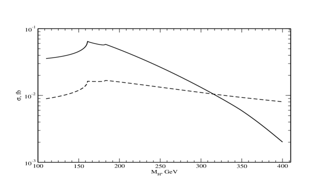
Figure 6: Annihilation channel: SANC at the one-loop level.

1. “Right” three-boson ($B\gamma H,\;B=\gamma,Z$) vertex, see Fig.6 of Ref. [3]. The diagram with $B=\gamma$ leads to a Coulomb singularity for the decay and production channels.

2. Boxes of T1 and T3 topologies with virtual $W$ boson, see Fig.15 of Ref. [1].

3. Box of T5 topology with virtual $Z$ boson, see Fig.16 of Ref. [1].

4. Associated $WW$ and $ZZ$ vertices of the topology BFB, see Fig.10 of Ref. [1].

As was motivated above, we keep the two Born diagrams of the kind shown in Fig. 1 Ref. [3].

Every FF is presented as the sum over the gauge index ($1=\xi_{\scriptscriptstyle{A}},2=\xi_{\scriptscriptstyle{Z}},3=\xi_{\scriptscriptstyle{W}}\equiv\xi,4=\mbox{without}\,\xi$):

$$F_{v(a)i}(-s,-t,-u)=\sum_{k=1,4}{F_{v(a)ik}(-s,-t,-u)}.$$ (5)

Obviously, $k=1$ does not contribute in massless case. FFs for $k=2,3,4$ are rather compact, they are shown in the next section.

2.3 One-loop form factors

In the limit $m_{f}\to 0$ FFs with the gauge index $2$ take a simple form:

$$F_{v32}(-s,-t,-u) = Q_{f}\frac{v_{f}^{2}+a_{f}^{2}}{2}\,F_{2}(-s,-t,-u)\,,$$

$$F_{v42}(-s,-t,-u) = Q_{f}\frac{v_{f}^{2}+a_{f}^{2}}{2}\,F_{2}(-s,-u,-t)\,,$$

$$F_{a32}(-s,-t,-u) = Q_{f}v_{f}\,a_{f}\,F_{2}(-s,-t,-u)\,,$$

$$F_{a42}(-s,-t,-u) = Q_{f}v_{f}\,a_{f}\,F_{2}(-s,-u,-t)\,,$$ (6)

where an auxiliary function was introduced:

$$F_{2}(Q^{2},T^{2},U^{2}) = \frac{s_{\scriptscriptstyle{W}}}{c_{\scriptscriptstyle{W}}^{3}}\frac{M_{\scriptscriptstyle{Z}}}{Q^{2}U^{2}}\biggl{\{}\left(M_{\scriptscriptstyle{Z}}^{2}+U^{2}\right)\frac{1}{U^{2}}\,C_{d_{0}c_{0}}(T^{2},U^{2},-M_{\scriptscriptstyle{H}}^{2};M_{\scriptscriptstyle{Z}})$$ (7)

$$+\left(M_{\scriptscriptstyle{Z}}^{2}+U^{2}\right)\left(M_{\scriptscriptstyle{H}}^{2}+U^{2}\right)\frac{1}{U^{2}}C_{0}(-M_{\scriptscriptstyle{H}}^{2},-m_{f}^{2},U^{2};M_{\scriptscriptstyle{Z}},M_{\scriptscriptstyle{Z}},m_{f})$$

$$+\left[Q^{2}-U^{2}+M_{\scriptscriptstyle{Z}}^{2}\left(1+\frac{Q^{2}}{U^{2}}+2\frac{U^{2}}{T^{2}+M_{\scriptscriptstyle{H}}^{2}}\right)\right]C_{0}(-M_{\scriptscriptstyle{H}}^{2},-m_{f}^{2},T^{2};M_{\scriptscriptstyle{Z}},M_{\scriptscriptstyle{Z}},m_{f})$$

$$-\frac{2Q^{2}}{T^{2}+M_{\scriptscriptstyle{H}}^{2}}\Big{[}B^{F}_{0}\big{(}-M_{\scriptscriptstyle{H}}^{2};M_{\scriptscriptstyle{Z}},M_{\scriptscriptstyle{Z}}\big{)}-B^{F}_{0}\big{(}T^{2};M_{\scriptscriptstyle{Z}},m_{f}\big{)}\Big{]}\biggr{\}},$$

with a combination of Passarino–Veltman functions which is explicitly free off fermionic mass singularities:

$$C_{d_{0}c_{0}}(T^{2},U^{2},-M_{\scriptscriptstyle{H}}^{2};M_{\scriptscriptstyle{Z}}) = \big{[}-T^{2}U^{2}-\big{(}T^{2}+U^{2}\big{)}M_{\scriptscriptstyle{Z}}^{2}\big{]}D_{0}(0,-m_{f}^{2},-M_{\scriptscriptstyle{H}}^{2},-m_{f}^{2},T^{2},U^{2};m_{f},m_{f},M_{\scriptscriptstyle{Z}},M_{\scriptscriptstyle{Z}})$$ (8)

$$-T^{2}C_{0}(0,-m_{f}^{2},T^{2};m_{f},m_{f},M_{\scriptscriptstyle{Z}})-U^{2}C_{0}(0,-m_{f}^{2},U^{2};m_{f},m_{f},M_{\scriptscriptstyle{Z}})\,.$$

The FFs with gauge index $4$ are:

$$F_{v34}(Q^{2})=F_{v44}(Q^{2})=2\,\sum_{i}\,s_{\scriptscriptstyle{W}}\,c_{i}\frac{m_{i}^{2}}{M_{\scriptscriptstyle{W}}}\left(4\frac{Q_{f}Q^{2}_{i}s_{\scriptscriptstyle{W}}^{2}}{Q^{2}}+\frac{v_{f}Q_{i}v_{i}}{c_{\scriptscriptstyle{W}}^{2}}\,\frac{1}{Q^{2}+M_{\scriptscriptstyle{Z}}^{2}}\right)F_{4i}\,,$$

$$F_{a34}(Q^{2})=F_{a44}(Q^{2})=2\,\sum_{i}\,s_{\scriptscriptstyle{W}}\,c_{i}\frac{m_{i}^{2}}{M_{\scriptscriptstyle{W}}}\left(\frac{a_{f}Q_{i}v_{i}}{c_{\scriptscriptstyle{W}}^{2}}\,\frac{1}{Q^{2}+M_{\scriptscriptstyle{Z}}^{2}}\right)F_{4i}\,,$$ (9)

with the auxiliary function,

$$F_{4i}(Q^{2}) = \left(\frac{1}{2}-2\frac{m^{2}_{i}}{Q^{2}+M_{\scriptscriptstyle{H}}^{2}}\right)C_{0}(0,-M_{\scriptscriptstyle{H}}^{2},Q^{2},m_{i},m_{i},m_{i})$$ (10)

$$+\frac{1}{Q^{2}+M_{\scriptscriptstyle{H}}^{2}}\left[1-\frac{Q^{2}}{Q^{2}+M_{\scriptscriptstyle{H}}^{2}}\Big{(}B^{F}_{0}\big{(}-M_{\scriptscriptstyle{H}}^{2};m_{i},m_{i}\big{)}-B^{F}_{0}\big{(}Q^{2};m_{i},m_{i}\big{)}\Big{)}\right],$$

The FFs with gauge index $3$ are more cumbersome:

$$F_{v33}(-s,-t,-u) = Q_{f}F_{q3}(-s)+v_{f}F_{va3}(-s)+F_{3}(-s,-t,-u)\,,$$

$$F_{v43}(-s,-t,-u) = Q_{f}F_{q3}(-s)+v_{f}F_{va3}(-s)+F_{3}(-s,-u,-t)\,,$$

$$F_{a33}(-s,-t,-u) = a_{f}F_{va3}(-s)+F_{3}(-s,-t,-u)\,,$$

$$F_{a43}(-s,-t,-u) = a_{f}F_{va3}(-s)+F_{3}(-s,-u,-t)\,,$$ (11)

and one needs three auxiliary functions to define them:

$$F_{q3}(Q^{2}) = 2\frac{s_{\scriptscriptstyle{W}}^{3}}{M_{\scriptscriptstyle{W}}}\biggl{\{}-2\frac{M_{\scriptscriptstyle{W}}^{2}}{Q^{2}}\left(4-\frac{M_{\scriptscriptstyle{H}}^{2}+6M_{\scriptscriptstyle{W}}^{2}}{Q^{2}+M_{\scriptscriptstyle{H}}^{2}}\right)C_{0}(0,-M_{\scriptscriptstyle{H}}^{2},Q^{2};M_{\scriptscriptstyle{W}},M_{\scriptscriptstyle{W}},M_{\scriptscriptstyle{W}})$$

$$+\frac{M_{\scriptscriptstyle{H}}^{2}+6M_{\scriptscriptstyle{W}}^{2}}{Q^{2}+M_{\scriptscriptstyle{H}}^{2}}\bigg{[}\frac{1}{Q^{2}+M_{\scriptscriptstyle{H}}^{2}}\bigg{(}B^{F}_{0}\big{(}-M_{\scriptscriptstyle{H}}^{2};M_{\scriptscriptstyle{W}},M_{\scriptscriptstyle{W}}\big{)}-B^{F}_{0}\big{(}Q^{2};M_{\scriptscriptstyle{W}},M_{\scriptscriptstyle{W}}\big{)}\bigg{)}-\frac{1}{Q^{2}}\bigg{]}\bigg{\}},$$

$$F_{va3}(Q^{2}) = \frac{s_{\scriptscriptstyle{W}}}{M_{\scriptscriptstyle{W}}}\bigg{\{}\frac{1}{Q^{2}+M_{\scriptscriptstyle{Z}}^{2}}\bigg{[}\bigg{(}\frac{1}{c_{\scriptscriptstyle{W}}^{2}}-6-\bigg{(}\frac{1}{c_{\scriptscriptstyle{W}}^{2}}-12c_{\scriptscriptstyle{W}}^{2}\bigg{)}\frac{M_{\scriptscriptstyle{Z}}^{2}}{Q^{2}+M_{\scriptscriptstyle{H}}^{2}}\bigg{)}$$

$$\times M_{\scriptscriptstyle{W}}^{2}C_{0}(0,-M_{\scriptscriptstyle{H}}^{2},Q^{2};M_{\scriptscriptstyle{W}},M_{\scriptscriptstyle{W}},M_{\scriptscriptstyle{W}})$$

$$+\bigg{(}\frac{1}{2c_{\scriptscriptstyle{W}}^{2}}-1+\bigg{(}\frac{1}{2c_{\scriptscriptstyle{W}}^{2}}-6c_{\scriptscriptstyle{W}}^{2}\bigg{)}\frac{M_{\scriptscriptstyle{Z}}^{2}}{Q^{2}+M_{\scriptscriptstyle{H}}^{2}}\bigg{)}$$

$$\times\bigg{(}\frac{M_{\scriptscriptstyle{Z}}^{2}}{Q^{2}+M_{\scriptscriptstyle{H}}^{2}}\bigg{(}B^{F}_{0}\big{(}-M_{\scriptscriptstyle{H}}^{2};M_{\scriptscriptstyle{W}},M_{\scriptscriptstyle{W}}\big{)}-B^{F}_{0}\big{(}Q^{2};M_{\scriptscriptstyle{W}},M_{\scriptscriptstyle{W}}\big{)}\bigg{)}+1\bigg{)}\bigg{]}$$

$$+\frac{1}{Q^{2}+M_{\scriptscriptstyle{H}}^{2}}\bigg{[}\bigg{(}\frac{1}{c_{\scriptscriptstyle{W}}^{2}}-2\bigg{)}M_{\scriptscriptstyle{W}}^{2}C_{0}(0,-M_{\scriptscriptstyle{H}}^{2},Q^{2};M_{\scriptscriptstyle{W}},M_{\scriptscriptstyle{W}},M_{\scriptscriptstyle{W}})$$

$$+\frac{M_{\scriptscriptstyle{Z}}^{2}}{Q^{2}+M_{\scriptscriptstyle{H}}^{2}}\bigg{(}-\frac{1}{2c_{\scriptscriptstyle{W}}^{2}}+6c_{\scriptscriptstyle{W}}^{2}+\bigg{(}1-\frac{1}{2c_{\scriptscriptstyle{W}}^{2}}\bigg{)}\frac{M_{\scriptscriptstyle{H}}^{2}}{M_{\scriptscriptstyle{Z}}^{2}}\bigg{)}$$

$$\times\bigg{(}B^{F}_{0}\big{(}-M_{\scriptscriptstyle{H}}^{2};M_{\scriptscriptstyle{W}},M_{\scriptscriptstyle{W}}\big{)}-B^{F}_{0}\big{(}Q^{2};M_{\scriptscriptstyle{W}},M_{\scriptscriptstyle{W}}\big{)}\bigg{)}-\frac{1}{2c_{\scriptscriptstyle{W}}^{2}}+1\bigg{]}\bigg{\}},$$

$$F_{3}(Q^{2},T^{2},U^{2}) = \frac{1}{2}s_{\scriptscriptstyle{W}}M_{\scriptscriptstyle{W}}\bigg{\{}\frac{1}{Q^{2}U_{s}^{4}}\bigg{[}\big{(}U^{2}+M_{\scriptscriptstyle{W}}^{2}\big{)}\bigg{(}Q^{2}\big{(}U^{2}+M_{\scriptscriptstyle{W}}^{2}\big{)}+M_{\scriptscriptstyle{W}}^{2}M_{\scriptscriptstyle{H}}^{2}\bigg{)}\,d_{0\rm{aux}}(Q^{2},U^{2})$$ (12)

$$+\bigg{(}\big{[}\big{(}U^{2}+M_{\scriptscriptstyle{W}}^{2}\big{)}M_{\scriptscriptstyle{W}}^{2}+Q^{2}T^{2}\big{]}M_{\scriptscriptstyle{H}}^{2}+2Q^{2}U^{2}M_{\scriptscriptstyle{W}}^{2}+Q^{2}\big{(}T^{2}-M_{\scriptscriptstyle{W}}^{2}\big{)}^{2}\bigg{)}\,d_{0\rm{aux}}(Q^{2},T^{2})$$

$$+Q_{s}^{4}C_{0}(-m_{\mu}^{2},-m_{\mu}^{2},Q^{2};M_{\scriptscriptstyle{W}},0,M_{\scriptscriptstyle{W}})$$

$$+\big{(}Q^{2}+M_{\scriptscriptstyle{H}}^{2}\big{)}\big{[}Q^{2}+2\big{(}U^{2}+M_{\scriptscriptstyle{W}}^{2}\big{)}\big{]}C_{0}(0,-M_{\scriptscriptstyle{H}}^{2},Q^{2};M_{\scriptscriptstyle{W}},M_{\scriptscriptstyle{W}},M_{\scriptscriptstyle{W}})$$

$$+\bigg{(}Q^{2}\big{(}T^{2}+M_{\scriptscriptstyle{H}}^{2}\big{)}+\big{(}U^{2}+M_{\scriptscriptstyle{W}}^{2}\big{)}(U^{2}-Q^{2})+2\frac{M_{\scriptscriptstyle{W}}^{2}Q^{2}U^{2}}{T^{2}+M_{\scriptscriptstyle{H}}^{2}}\bigg{)}$$

$$\times C_{0}(-M_{\scriptscriptstyle{H}}^{2},-m_{\mu}^{2},T^{2};M_{\scriptscriptstyle{W}},M_{\scriptscriptstyle{W}},0)$$

$$-\big{(}U^{2}+M_{\scriptscriptstyle{H}}^{2}\big{)}\big{(}U^{2}+M_{\scriptscriptstyle{W}}^{2}\big{)}C_{0}(-M_{\scriptscriptstyle{H}}^{2},-m_{\mu}^{2},U^{2};M_{\scriptscriptstyle{W}},M_{\scriptscriptstyle{W}},0)$$

$$+T^{2}\big{(}Q^{2}+U^{2}+M_{\scriptscriptstyle{W}}^{2}\big{)}C_{0}(0,-m_{\mu}^{2},T^{2};M_{\scriptscriptstyle{W}},M_{\scriptscriptstyle{W}},0)$$

$$+U^{2}(U^{2}+M_{\scriptscriptstyle{W}}^{2})C_{0}(0,-m_{\mu}^{2},U^{2};M_{\scriptscriptstyle{W}},M_{\scriptscriptstyle{W}},0)\bigg{]}$$

$$+\frac{2}{U^{2}}\,\frac{1}{T^{2}+M_{\scriptscriptstyle{H}}^{2}}\bigg{(}B^{F}_{0}\big{(}-M_{\scriptscriptstyle{H}}^{2};M_{\scriptscriptstyle{W}},M_{\scriptscriptstyle{W}}\big{)}-B^{F}_{0}\big{(}T^{2};M_{\scriptscriptstyle{W}},0\big{)}\bigg{)}\bigg{\}}.$$

Here two two more auxiliary functions are introduced:

$$d_{0\rm{aux}}(Q^{2},T^{2})=d_{0}(-m_{\mu}^{2},-m_{\mu}^{2},0,-M_{\scriptscriptstyle{H}}^{2},Q^{2},T^{2};M_{\scriptscriptstyle{W}},0,M_{\scriptscriptstyle{W}},M_{\scriptscriptstyle{W}})\,.$$

$$d_{0\rm{aux}}(Q^{2},U^{2})=d_{0}(-m_{\mu}^{2},-m_{\mu}^{2},-M_{\scriptscriptstyle{H}}^{2},0,Q^{2},U^{2};M_{\scriptscriptstyle{W}},0,M_{\scriptscriptstyle{W}},M_{\scriptscriptstyle{W}})\,,$$ (13)

The complete analytic results were presented in the literature earlier, see e.g. Ref. [10] and references therein. The aim of presentation of this section is to show once typical SANC result for the FF in terms of only scalar Passarino–Veltman functions.

2.4 Helicity amplitudes

In this section we present the HAs for all three channels.

2.4.1 Annihilation channel $\bar{f}f\to\gamma H$

In this case permutation of 4-momenta with respect to CA (2.1) is very simple.

Figure 3: Schematic representation of one-loop Feynman diagrams for the annihilation channel.

Convert for channel $\bar{f}(p_{1})f(p_{2})\to\gamma(p3)H(p4)$:

$$\begin{array}[]{llll}&p_{1}&\to&~{}~{}p_{1},\\ &p_{2}&\to&~{}~{}p_{2},\\ &p_{3}&\to&-p_{3},\\ &p_{4}&\to&-p_{4}.\\ \end{array}$$

The set of corresponding HAs for the case reads:

$${\cal H}_{\pm\pm\pm} = \mp k_{0}\biggl{[}\frac{-Z_{4}(M_{\scriptscriptstyle{H}})\beta_{+}/2+s\beta^{2}}{Z_{1}(m_{f})Z_{2}(m_{f})}F_{v1}(-s,-t,-u)$$

$$\mp s\beta F_{a1}(-s,-t,-u)-\beta_{+}\left(F_{v2}(-s,-t,-u)\mp F_{a2}(-s,-t,-u)\right)$$

$$+m_{f}\left(F_{v3}(-s,-t,-u)\mp\beta F_{a3}(-s,-t,-u)\right)+m_{f}\left(F_{v4}(-s,-t,-u)\pm\beta F_{a4}(-s,-t,-u)\right)\biggr{]},$$

$${\cal H}_{\pm\pm\mp} = \pm k_{0}\biggl{[}\frac{-Z_{4}(M_{\scriptscriptstyle{H}})\beta_{-}/2+s\beta^{2}}{Z_{1}(m_{f})Z_{2}(m_{f})}F_{v1}(-s,-t,-u)$$

$$\mp s\beta F_{a1}(-s,-t,-u)-\beta_{-}\left(F_{v2}(-s,-t,-u)\pm F_{a2}(-s,-t,-u)\right)$$

$$+m_{f}\left(F_{v3}(-s,-t,-u)\mp\beta F_{a3}(-s,-t,-u)\right)+m_{f}\left(F_{v4}(-s,-t,-u)\pm\beta F_{a4}(-s,-t,-u)\right)\biggr{]},$$

$${\cal H}_{\pm\mp\pm} = -k_{+}\biggl{[}\frac{2m_{f}}{s}\frac{Z_{4}(M_{\scriptscriptstyle{H}})}{Z_{1}(m_{f})Z_{2}(m_{f})}F_{v1}(-s,-t,-u)+\frac{4m_{f}}{s}\left(F_{v2}(-s,-t,-u)\mp F_{a2}(-s,-t,-u)\right)$$

$$-\beta_{+}\left(F_{v3}(-s,-t,-u)\pm\beta F_{a3}(-s,-t,-u)\right)-\beta_{-}\left(F_{v4}(-s,-t,-u)\pm\beta F_{a4}(-s,-t,-u)\right)\biggr{]},$$

$${\cal H}_{\pm\mp\mp} = -k_{-}\biggl{[}\frac{2m_{f}}{s}\frac{Z_{4}(M_{\scriptscriptstyle{H}})}{Z_{1}(m_{f})Z_{2}(m_{f})}F_{v1}(-s,-t,-u)+\frac{4m_{f}}{s}\left(F_{v2}(-s,-t,-u)\pm F_{a2}(-s,-t,-u)\right)$$

$$-\beta_{-}\left(F_{v3}(-s,-t,-u)\pm\beta F_{a3}(-s,-t,-u)\right)-\beta_{+}\left(F_{v4}(-s,-t,-u)\pm\beta F_{a4}(-s,-t,-u)\right)\biggr{]},$$

where the coefficients

$$k_{0}=\sin\vartheta_{\gamma}\frac{s_{h}}{2\sqrt{2}}\,,\qquad k_{\pm}=c_{\pm}\frac{s_{h}\sqrt{s}}{4\sqrt{2}}\,,$$ (15)

with

$$s_{h}=s-M_{\scriptscriptstyle{H}}^{2}\,,\qquad c_{\pm}=1\pm\cos\vartheta_{\gamma}\,,\qquad\beta_{\pm}=1\pm\beta\,,\qquad\beta={\sqrt{\lambda(s,m_{f}^{2},m_{f}^{2})}}/{s}\,,$$ (16)

and fermionic propagators and $t,u$ invariants are:

$$Z_{1}(m_{f}) = \frac{1}{2}Z_{4}(M_{\scriptscriptstyle{H}})\left(1+\beta\cos{\vartheta_{\gamma}}\right),$$

$$Z_{2}(m_{f}) = \frac{1}{2}Z_{4}(M_{\scriptscriptstyle{H}})\left(1-\beta\cos{\vartheta_{\gamma}}\right),$$

$$t = m_{f}^{2}-Z_{2}(m_{f}),$$

$$u = m_{f}^{2}-Z_{1}(m_{f}).$$ (17)

Here $Z_{4}(M_{\scriptscriptstyle{H}})=s_{h}$ and $\vartheta_{\gamma}$ is the cms angle of the produced photon (angle between 4-momenta $\vec{p}_{2}$ and $\vec{p}_{3}$).

2.4.2 Decay channel $H\to\gamma f\bar{f}$

The 4-momenta permutations for this channel are chosen as follows.

Figure 4: Schematic representation of one-loop Feynman diagram for the decay channel.

Convert for channel $H(p_{2})\to\gamma(p_{1})f(p_{3})\bar{f}(p_{4})$:

$$\begin{array}[]{llll}&p_{1}&\to&-p_{3},\\ &p_{2}&\to&-p_{4},\\ &p_{3}&\to&-p_{1},\\ &p_{4}&\to&~{}~{}p_{2}.\end{array}$$

The HAs for this channel are somewhat similar to the annihilation ones:

$${\cal H}_{\pm\pm\pm} = k_{0}\biggl{[}\frac{\beta_{-}Z_{2}(M_{\scriptscriptstyle{H}})/2+s\beta^{2}}{Z_{3}(m_{f})Z_{4}(m_{f})}F_{v1}(-s,-t,-u)\pm\beta sF_{a1}(-s,-t,-u)$$

$$-\beta_{-}\left(F_{v2}(-s,-t,-u)\mp F_{a2}(-s,-t,-u)\right)$$

$$+m_{f}\left(F_{v3}(-s,-t,-u)\pm\beta F_{a3}(-s,-t,-u)\right)+m_{f}\left(F_{v4}(-s,-t,-u)\mp\beta F_{a4}(-s,-t,-u)\right)\biggr{]},$$

$${\cal H}_{\pm\mp\mp} = k_{0}\biggl{[}\frac{\beta_{+}Z_{2}(M_{\scriptscriptstyle{H}})/2+s\beta^{2}}{Z_{3}(m_{f})Z_{4}(m_{f})}F_{v1}(-s,-t,-u)\mp\beta sF_{a1}(-s,-t,-u)$$

$$-\beta_{+}\left(F_{v2}(-s,-t,-u)\mp F_{a2}(-s,-t,-u)\right)$$

$$+m_{f}\left(F_{v3}(-s,-t,-u)\mp\beta F_{a3}(-s,-t,-u)\right)+m_{f}\left(F_{v4}(-s,-t,-u)\pm\beta F_{a4}(-s,-t,-u)\right)\biggr{]},$$

$${\cal H}_{\pm\mp\pm} = k_{+}\biggl{[}\mp\frac{2m_{f}}{s}\frac{Z_{2}(M_{\scriptscriptstyle{H}})}{Z_{3}(m_{f})Z_{4}(m_{f})}F_{v1}(-s,-t,-u)\pm\frac{4m_{f}}{s}\left(F_{v2}(-s,-t,-u)\mp F_{a2}(-s,-t,-u)\right)$$

$$\mp\beta_{+}\left(F_{v3}(-s,-t,-u)\pm\beta F_{a3}(-s,-t,-u)\right)\mp\beta_{-}\left(F_{v4}(-s,-t,-u)\pm\beta F_{a4}(-s,-t,-u)\right)\biggr{]},$$

$${\cal H}_{\pm\pm\mp} = k_{-}\biggl{[}\mp\frac{2m_{f}}{s}\frac{Z_{2}(M_{\scriptscriptstyle{H}})}{Z_{3}(m_{f})Z_{4}(m_{f})}F_{v1}(-s,-t,-u)\pm\frac{4m_{f}}{s}\left(F_{v2}(-s,-t,-u)\mp F_{a2}(-s,-t,-u)\right)$$

$$\mp\beta_{-}\left(F_{v3}(-s,-t,-u)\mp\beta F_{a3}(-s,-t,-u)\right)\mp\beta_{+}\left(F_{v4}(-s,-t,-u)\mp\beta F_{a4}(-s,-t,-u)\right)\biggr{]},$$

where the coefficients

$$k_{0} = \sin\vartheta_{f}\frac{Z_{2}(M_{\scriptscriptstyle{H}})}{2\sqrt{2}}\,,$$

$$k_{\pm} = c_{\pm}\frac{Z_{2}(M_{\scriptscriptstyle{H}})\sqrt{s}}{4\sqrt{2}}\,,$$

$$\beta_{\pm} = 1\pm\beta\,,\qquad\beta=\sqrt{1-\frac{4m_{f}^{2}}{s}}.$$ (19)

and the propagators of radiating fermions and $s,t,u$ invariants are:

$$Z_{3}(m_{f}) = \frac{1}{2}Z_{2}(M_{\scriptscriptstyle{H}})\left(1+\beta\cos{\vartheta_{f}}\right),$$

$$Z_{4}(m_{f}) = \frac{1}{2}Z_{2}(M_{\scriptscriptstyle{H}})\left(1-\beta\cos{\vartheta_{f}}\right),$$

$$s = M^{2}_{f\bar{f}}\,,$$

$$t = m_{f}^{2}+Z_{4}(m_{f}),$$

$$u = m_{f}^{2}+Z_{3}(m_{f}).$$ (20)

with $Z_{2}(M_{\scriptscriptstyle{H}})=M_{\scriptscriptstyle{H}}^{2}-s$ and $\vartheta_{f}$ being the fermionic angle $(\vec{p}_{3},\vec{p}_{1})$ in the rest frame of compound $(\vec{p}_{3},\vec{p}_{4})$.

2.4.3 $H$ production channel $e\gamma\to eH$

For this channel we present HAs for two cases: for limit $m_{f}\to 0$ and exact in $m_{f}$.

Figure 5: Schematic representation of one-loop Feynman diagrams for $e\gamma$ channel.

Convert for channel $\gamma(p_{1})e(p_{2})\to e(p_{3})H(p_{4})$ is:

$$\begin{array}[]{lllll}&&p_{1}&\to&-p_{3},\\ &&p_{2}&\to&~{}~{}p_{2},\\ &&p_{3}&\to&~{}~{}p_{1},\\ &&p_{4}&\to&-p_{4}.\end{array}$$

The small mass limit is remarkably compact:

$${\cal H}_{\pm\pm\pm} = \pm k_{1}\left[F_{v4}(-s,-t,-u)\mp F_{a4}(-s,-t,-u)\right],$$

$${\cal H}_{\mp\pm\pm} = \mp k_{2}\left[F_{v3}(-s,-t,-u)\mp F_{a3}(-s,-t,-u)\right],$$

$${\cal H}_{\mp\mp\pm} = k_{3}\biggl{[}\frac{M_{\scriptscriptstyle{H}}^{2}}{Z_{3}(m_{e})}F_{v1}(-s,-t,-u)\pm kF_{a1}(-s,-t,-u)+2s\left(F_{v2}(-s,-t,-u)\pm F_{a2}(-s,-t,-u)\right)\biggr{]},$$

$${\cal H}_{\mp\pm\mp} = k_{3}\biggl{[}\left(\frac{s_{h}}{Z_{3}(m_{e})}-1\right)F_{v1}(-s,-t,-u)\pm kF_{a1}(-s,-t,-u)\biggr{]},$$ (21)

with the coefficients

$$k = c_{-}\frac{ss_{h}}{2},\qquad\qquad\qquad k_{1}=\sin\frac{\vartheta_{f}}{2}s\sqrt{\frac{s_{h}}{2}},$$

$$k_{2} = c_{+}\sin\frac{\vartheta_{f}}{2}\frac{\left(s_{h}\right)^{{3}/{2}}}{2\sqrt{2}},\qquad k_{3}=\cos\frac{\vartheta_{f}}{2}\sqrt{\frac{s_{h}}{2s}},$$ (22)

The exact in $m_{f}$ fermionic propagators are:

$$Z_{2}(m_{f}) = s-m_{f}^{2}\,,$$

$$Z_{3}(m_{f}) = \frac{Z_{2}(m_{f})}{2s}\left[s+m_{f}^{2}-M_{\scriptscriptstyle{H}}^{2}+\sqrt{\lambda(s,m_{f}^{2},M_{\scriptscriptstyle{H}}^{2})}\cos\vartheta_{f}\right].$$ (23)

The Mandelstam variables transform as follows:

$$s \rightarrow \frac{1}{2}\left[\left(s-\frac{M_{\scriptscriptstyle{H}}^{2}m_{f}^{2}}{s}-M_{\scriptscriptstyle{H}}^{2}-2m_{f}^{2}+\frac{m_{f}^{4}}{s}\right)-\frac{s-m_{f}^{2}}{s}\sqrt{\lambda(s,m_{f}^{2},M_{\scriptscriptstyle{H}}^{2})}\cos\vartheta_{f}\right],$$

$$t \rightarrow s,$$

$$u \rightarrow \frac{1}{2}\left[\left(s+\frac{M_{\scriptscriptstyle{H}}^{2}m_{f}^{2}}{s}-M_{\scriptscriptstyle{H}}^{2}-2m_{f}^{2}-\frac{m_{f}^{2}}{s}\right)+\frac{s-m_{f}^{2}}{s}\sqrt{\lambda(s,m_{f}^{2},M_{\scriptscriptstyle{H}}^{2})}\cos\vartheta_{f}\right].$$ (24)

The quantity

$$Z_{4}(M_{\scriptscriptstyle{H}}) = \frac{Z_{2}(m_{f})}{2s}\left[s-m_{f}^{2}+M_{\scriptscriptstyle{H}}^{2}-\sqrt{\lambda(s,m_{f}^{2},M_{\scriptscriptstyle{H}}^{2})}\cos\vartheta_{f}\right],$$ (25)

represents a would-be Higgs boson propagator, which appears only in numerator, since Higgs does not radiate photons. For $Z_{2}(m_{f})$ and $Z_{4}(M_{\scriptscriptstyle{H}})$ we use here massless expressions, while for $Z_{3}(m_{f})$ — exact one, since it develops logarithmic mass singularity. For the massive case below, we use all expressions exact in masses. Also important quantities for this channel are:

$$N_{\pm}=\sqrt{m_{f}^{2}+E_{2}E_{3}\mp p_{2}p_{3}}\,.$$ (26)

In massless case only $N_{+}$ contributes and its limit is

$$N_{+}=\sqrt{\displaystyle\frac{s_{h}}{2}}\,.$$ (27)

The fully massive case has the following form:

$$\cal{H}_{\pm\pm\pm} = \sin{\frac{\vartheta_{f}}{2}}\biggl{[}\pm\frac{1}{Z_{2}(m_{f})Z_{3}(m_{f})}\bigg{(}\sqrt{s}\left[M_{\scriptscriptstyle{H}}^{2}-m_{f}^{2}\left(4+r_{d_{2}}\cos{\vartheta_{f}}\right)\right]N_{+}$$ (28)

$$+\frac{m_{f}}{2}\left(3s_{h}+m_{f}^{2}(9-r_{d_{1}})+\left[s_{h}+m_{f}^{2}(3+r_{d_{1}})\right]\cos{\vartheta_{f}}\right)N_{-}\bigg{)}F_{v1}(-s,-t,-u)$$

$$-s_{m}c_{+}\left[\frac{\sqrt{s}}{2}(-2+r_{d_{1}})N_{+}-m_{f}N_{-}\right]F_{a1}(-s,-t,-u)$$

$$\pm 2\left(\sqrt{s}N_{+}-m_{f}N_{-}\right)\left(F_{v2}(-s,-t,-u)\mp F_{a2}(-s,-t,-u)\right)$$

$$\mp\frac{m_{f}}{2}\Big{[}\sqrt{s}\left(4-r_{d_{1}}+r_{d_{3}}\cos{\vartheta_{f}}\right)N_{+}-m_{f}\left(4-r_{d_{1}}c_{-}\right)N_{-}\Big{]}F_{v3}(-s,-t,-u)$$

$$+\frac{m_{f}}{2}\Big{[}\sqrt{s}\left(r_{d_{1}}-r_{d_{3}}\cos{\vartheta_{f}}\right)N_{+}-m_{f}r_{d_{1}}c_{-}N_{-}\Big{]}F_{a3}(-s,-t,-u)$$

$$\mp\left[2\sqrt{s}m_{f}N_{+}-(s+m_{f}^{2})N_{-}\right]F_{v4}(-s,-t,-u)-s_{m}N_{-}F_{a4}(-s,-t,-u)\biggr{]},$$

$$\cal{H}_{\mp\pm\pm} = \sin{\frac{\vartheta_{f}}{2}}c_{+}\biggl{[}\pm\frac{1}{Z_{2}(m_{f})Z_{3}(m_{f})}\left(\frac{\sqrt{s}}{2}\left[s_{h}+m_{f}^{2}(3+r_{d_{1}})\right]N_{+}-sm_{f}r_{d_{2}}N_{-}\right)F_{v1}(-s,-t,-u)$$ (29)

$$+\left(\frac{\sqrt{s}}{2}\left[s_{h}+m_{f}^{2}(3-r_{d_{1}})\right]N_{+}-s_{m}m_{f}N_{-}\right)F_{a1}(-s,-t,-u)$$

$$\pm\frac{1}{2}\left(\sqrt{s}m_{f}r_{d_{1}}N_{+}-sr_{d_{3}}N_{-}\right)\left(F_{v3}(-s,-t,-u)\mp F_{a3}(-s,-t,-u)\right)\biggr{]},$$

$$\cal{H}_{\mp\mp\pm} = \cos{\frac{\vartheta_{f}}{2}}\biggl{[}\frac{1}{Z_{2}(m_{f})Z_{3}(m_{f})}\biggl{(}\frac{m_{f}}{2}\bigl{(}3s_{h}+m_{f}^{2}(9-r_{d_{1}})$$ (30)

$$-\left[s_{h}+m_{f}^{2}(3+r_{d_{1}})\right]\cos{\vartheta_{f}}\bigr{)}N_{+}+\sqrt{s}\left[M_{\scriptscriptstyle{H}}^{2}-m_{f}^{2}(4-r_{d_{2}}\cos{\vartheta_{f}})\right]N_{-}\biggr{)}F_{v1}(-s,-t,-u)$$

$$\mp c_{-}\left(s_{m}m_{f}N_{+}-\frac{\sqrt{s}}{2}\left[s_{h}+m_{f}^{2}(3-r_{d_{1}})\right]N_{-}\right)F_{a1}(-s,-t,-u)$$

$$-2\left(m_{f}N_{+}-\sqrt{s}N_{-}\right)\left(F_{v2}(-s,-t,-u)\pm F_{a2}(-s,-t,-u)\right)$$

$$+\frac{m_{f}}{2}\Bigl{[}m_{f}\left(4-r_{d_{1}}c_{+}\right)N_{+}-\sqrt{s}\left(4-r_{d_{1}}-r_{d_{3}}\cos{\vartheta_{f}}\right)N_{-}\Bigr{]}F_{v3}(-s,-t,-u)$$

$$\pm\frac{m_{f}}{2}\Bigl{[}m_{f}r_{d_{1}}c_{+}N_{+}-\sqrt{s}\left(r_{d_{1}}+r_{d_{3}}\cos{\vartheta_{f}}\right)N_{-}\Bigr{]}F_{a3}(-s,-t,-u)$$

$$+\left[(s+m_{f}^{2})N_{+}-2\sqrt{s}m_{f}N_{-}\right]F_{v4}(-s,-t,-u)\pm s_{m}N_{+}F_{a4}(-s,-t,-u)\biggr{]},$$

$${\cal H}_{\mp\pm\mp} = \cos{\frac{\vartheta_{f}}{2}}c_{-}\biggl{[}\frac{1}{Z_{2}(m_{f})Z_{3}(m_{f})}\biggl{(}-sm_{f}r_{d_{2}}N_{+}+\frac{\sqrt{s}}{2}\left[s_{h}+m_{f}^{2}(3+r_{d_{1}})\right]N_{-}\biggr{)}F_{v1}(-s,-t,-u)$$ (31)

$$\mp\left(s_{m}m_{f}N_{+}-\frac{\sqrt{s}}{2}\left[s_{h}+m_{f}^{2}(3-r_{d_{1}})\right]N_{-}\right)F_{a1}(-s,-t,-u)$$

$$-\frac{1}{2}\left(sr_{d_{3}}N_{+}-\sqrt{s}m_{f}r_{d_{1}}N_{-}\right)\left(F_{v3}(-s,-t,-u)\mp F_{a3}(-s,-t,-u)\right)\biggr{]},$$

where

$$s_{m}=s-m_{f}^{2}\,,\quad r_{d_{1}}=3-\frac{M_{\scriptscriptstyle{H}}^{2}-m_{f}^{2}}{s}\,,\quad r_{d_{2}}=2-\frac{M_{\scriptscriptstyle{H}}^{2}-2m_{f}^{2}}{s}\,,\quad r_{d_{3}}=1-\frac{M_{\scriptscriptstyle{H}}^{2}-3m_{f}^{2}}{s}\,$$ (32)

and $\vartheta_{f}$ is the cms angle of the final fermion.

3 Numerical results and comparison

In this section we present results of numerical calculations and comparisons with other groups.

3.1 Annihilation channel $f\bar{f}\to\gamma H$

There are many papers devoted to this channel, see for example Refs. [8]–[10] and references therein. It is highly non-trivial to realize a tuned comparison of the numerical results, since the authors do not present the list of input parameters, do not specify calculational scheme, although stating an agreement among themselves. Eventually, we found the best to compare with newest paper Ref. [10], namely with Fig.2, showing the $M_{\scriptscriptstyle{H}}$ dependence of the total cross section for two values of $\sqrt{s}$=500 (solid line) and 1500 GeV (dashed line). As can be judged from comparison of their figures with ours, there is a qualitative agreement of the cross sections. One should emphasize that we did not find in Ref. [10] which value of the top quark mass on which we observed quite a strong dependence.

For example, at $\sqrt{s}$=500 GeV and $M_{\scriptscriptstyle{H}}$=300 GeV, the cross section equals 1.32$\cdot 10^{-2}$ fb for $m_{t}=174.2$ GeV and 1.89$\cdot 10^{-2}$ fb for $m_{t}=140$ GeV.

 

Note, that all the numerical results of this section are produced with the so-called Standard SANC INPUT (section 6.2.3 of Ref. [3]).

3.2 Decay channel $H\to f\bar{f}\gamma$

For the decay channel we did not find in the literature complete one-loop calculations. We present here numerical results for the $H\to\mu^{+}\mu^{-}\gamma$ decay channel for $M_{\scriptscriptstyle{H}}=150$ GeV.

$\bullet$ GRACE, CompHEP and SANC at the Born level

The results of the comparison for the total width in the Born approximation in GeV between GRACE Ref. [6] CompHEP Ref. [5] and SANC are shown in the Table 1. Here the input parameters are as in CompHEP.

$E_{\gamma}$, GeV	$\Gamma$, GeV, [6]	$\Gamma$, GeV [5]	$\Gamma$, GeV, SANC
70	2.0490(1)	2.0489(1)	2.0491(1)	$\cdot 10^{-9}$
50	1.4187(1)	1.4189(1)	1.4188(1)	$\cdot 10^{-8}$
10	1.0029(1)	1.0030(1)	1.0030(1)	$\cdot 10^{-7}$
1	2.6265(2)	2.6266(1)	2.6264(1)	$\cdot 10^{-7}$
0.1	4.3329(2)	4.3325(1)	4.3326(1)	$\cdot 10^{-7}$
0.01	unstable	unstable	6.0474(1)	$\cdot 10^{-7}$

Table 1: Comparison for the total width between Refs. [6], [5] and SANC in the Born approximation.

Note, that SANC produces stable results up to very small photon energies which is mandatory to have correct description of soft and hard radiations.

$\bullet$ SANC at the Born and one-loop levels

In Fig. 7 the fermion-antifermion invariant mass distribution $d\Gamma/dM_{\mu^{+}\mu^{-}}$ is demonstrated.

Figure 7: Invariant mass distribution, Born (dashed) and one-loop levels (solid line).

Two peaks due to $\gamma$ and $Z$ exchanges, are distinctly seen. The Coulomb peak region usually does not represent any interest and should be cut out.

In Table 2, the partial width is shown in dependence on two cuts values, $s_{q\rm min,max},\;s_{q}=M_{\mu^{+}\mu^{-}}$ in the Born and one-loop approximation in two schemes $\alpha$ and $G_{\mu}$.

N	$s_{q\rm min}$	$s_{q\rm max}$	$\Gamma^{\rm{Born}}\cdot 10^{-8}$	$\Gamma^{\rm{Born+1-loop}}\cdot 10^{-6}$
			$\alpha$ scheme
1	$2m_{\mu}$	148.997	23.499	1.7536
2	$2m_{\mu}$	139.642	8.9737	1.6239
3	$M_{\scriptscriptstyle{Z}}-40$	$M_{\scriptscriptstyle{Z}}+40$	5.5040	1.2443
4	$M_{\scriptscriptstyle{Z}}-20$	$M_{\scriptscriptstyle{Z}}+20$	2.0188	1.1822
			$G_{\mu}$ scheme
1	$2m_{\mu}$	148.997	24.325	1.8152
2	$2m_{\mu}$	139.642	9.2891	1.6810
3	$M_{\scriptscriptstyle{Z}}-40$	$M_{\scriptscriptstyle{Z}}+40$	5.6975	1.2880
4	$M_{\scriptscriptstyle{Z}}-20$	$M_{\scriptscriptstyle{Z}}+20$	2.0898	1.2238

Table 2: SANC at the Born and one-loop levels.

All parameters and numbers are in GeV. Two first $s_{q\rm max}$ are calculated in terms of $E_{\gamma}$ cut by the equation $s^{2}_{q\rm max}=M_{\scriptscriptstyle{H}}^{2}-2M_{\scriptscriptstyle{H}}E_{\gamma}$ for $E_{\gamma}$=1 and 10 GeV, correspondingly. As seen, the major part of the one-loop decay width is due to $Z$ resonance.

$\bullet$ SANC in the resonance approximation at one-loop level

The latter observation justifies to an extent the usual approach to the calculation of this decay, the one-loop resonance approximation, which realized for example in PITHYA Ref. [7]:

$$\Gamma^{\rm{Res~{}1-loop}}_{H\to\mu^{+}\mu^{-}\gamma}=\frac{\Gamma^{\rm{1-loop}}_{H\to Z\gamma}{\Gamma^{\rm{1-loop}}_{Z\to\mu^{+}\mu^{-}}}}{\Gamma_{\scriptscriptstyle{Z}}}.$$ (33)

In Table 3, the total width is shown in dependence on cut value, $s_{q\rm min}$ in the resonance one-loop and in the complete one-loop approximations, again in two schemes $\alpha$ and $G_{\mu}$, here, however, without Born amplitude.

$s_{q{\rm min}}$, GeV	$\Gamma^{\rm{Res~{}1-loop}}\cdot 10^{-6}$ GeV		$\Gamma^{\rm{1-loop}}\cdot 10^{-6}$ GeV
	$\alpha$	$G_{\mu}$	$\alpha$	$G_{\mu}$
$2m_{\mu}$	1.17006	1.2112	1.54394	1.59822
1	1.17006	1.2112	1.45652	1.50773
10	1.17006	1.2112	1.29776	1.34339
30	1.16981	1.2109	1.22548	1.26857
50	1.16771	1.2088	1.19604	1.23809
70	1.15659	1.1973	1.17259	1.21381

Table 3: SANC, Resonance one-loop and complete one-loop approximations.

Comparing columns computed in the same schemes, we see that the resonance approximation works with percent accuracy for strong cuts (50,70) GeV.

3.3 Channel $e\gamma\to eH$

There is also reach literature devoted to this process (see, for example Refs. [11]–[12] and references therein).

We attempted a semi-tuned comparison of the total cross sections between Table I of Ref. [11] and SANC for three cms energies $\sqrt{s}=500,\;1000,\;1500\;$GeV and wide range of Higgs mass: 110 GeV$\leq M_{\scriptscriptstyle{H}}\leq$ 400 GeV. We tried to use all their masses we manage to find in the paper and convention of coupling of the “almost on-shell photon”.

$M_{\scriptscriptstyle{H}}/\sqrt{s}$	500			1000			1500
	SANC	[11]	$\delta$	SANC	[11]	$\delta$	SANC	[11]	$\delta$
80	8.40	8.38	-0.2	9.31	9.29	-0.2	9.76	9.74	-0.2
100	8.85	8.85	0	9.95	9.94	-0.1	10.48	10.5	-0.2
120	9.77	9.80	0.3	11.16	11.2	0.4	11.80	11.8	0
140	11.76	11.8	0.3	13.68	13.7	0.1	14.52	14.6	0.6
160	20.91	21.1	0.9	24.82	25.0	0.7	26.48	26.6	0.5
180	20.67	20.9	1.1	25.04	25.3	1.0	26.81	27.0	0.7
200	16.99	17.2	1.2	21.05	21.2	0.7	22.64	22.8	0.7
300	5.90	5.97	1.2	8.44	8.53	1.0	9.33	9.43	1.1
400	1.64	1.64	0	2.74	2.78	1.5	3.15	3.18	1.0

Table 4: $H$ production channel, SANC and Ref. [11].

In the Table we show total cross sections $\sigma$ and relative difference $\delta$ between two calculations ($\delta={\sigma\cite[cite]{[\@@bibref{}{Gabrielli:1997ix}{}{}]}}/{\sigma[\rm{SANC}]}-1,\,(\%)$). As seen, the difference in the vast majority of points is below 1% and shows up irregular behavior pointing to its numerical origin (our numbers are calculated with real*16). Given these observations, we consider the two results to be in a very good agreement.

References

- [1] A. Andonov et al., Comput. Phys. Commun. 174 (2006) 481–517.
- [2] SANC servers: Dubna — http://sanc.jinr.ru, CERN — http://pcphsanc.cern.ch.
- [3] D. Bardin, S. Bondarenko, L. Kalinovskaya, G. Nanava, L. Rumyantsev and W. von Schlippe, SANCnews: Sector f f b b, hep-ph/0506120.
- [4] J. A. M. Vermaseren, New features of FORM, math-ph/0010025.
- [5] E. Boos et al. [CompHEP Collaboration], Nucl. Instrum. Meth. A 534 (2004) 250.
- [6] F. Yuasa et al., Prog. Theor. Phys. Suppl. 138 (2000) 18 [arXiv:hep-ph/0007053].
- [7] T. Sjostrand, S. Mrenna and P. Skands, JHEP 0605 (2006) 026.
- [8] A. Barroso, J. Pulido and J. C. Romao, Nucl. Phys. B 267 (1986) 509.
- [9] A. Abbasabadi, D. Bowser-Chao, D. A. Dicus and W. W. Repko, Phys. Rev. D 52 (1995) 3919.
- [10] A. Djouadi, V. Driesen, W. Hollik and J. Rosiek, Nucl. Phys. B 491 (1997) 68
- [11] E. Gabrielli, V. A. Ilyin and B. Mele, Phys. Rev. D 56 (1997) 5945; [Erratum-ibid. D 58 (1998) 119902].
- [12] A. T. Banin, I. F. Ginzburg and I. P. Ivanov, Phys. Rev. D 59 (1999) 115001.