Diffractive Excitation of Heavy Flavors: Leading Twist Mechanisms

Abstract

Diffractive production of heavy flavors is calculated within the light-cone dipole approach. Novel leading twist mechanisms are proposed, which involve both short and long transverse distances inside the incoming hadron. Nevertheless, the diffractive cross section turns out to be sensitive to the primordial transverse momenta of projectile gluons, rather than to the hadronic size. Our calculations agree with the available data for diffractive production of charm and beauty, and with the observed weak variation of the diffraction-to-inclusive cross section ratios as function of the hard scale.

I Introduction

Diffraction is usually viewed as shadow of inelastic processes. This idea originated from optics helped considerably in the interpretation of data on elastic hadronic scattering. The understanding of the mechanisms of inelastic diffraction came with the pioneering works of Glauber glauber , Feinberg and Pomeranchuk f-p , Good and Walker g-w . If the incoming plane wave contains components interacting differently with the target, the outgoing wave will have a different composition, i.e. besides elastic scattering a new state will be created (e.g. see in brazil ). An optical analogy for inelastic diffraction would be a change of the light polarization after passing through a polarizer which absorbs differently two linear polarizations.

Thus, inelastic diffraction of hadrons should also be treated as a shadow, it emerges due to difference of shadows produced by different inelastic processes (in this respect a study of the structure function i-s of a shadow might look questionable). Some of the shadows from different hadronic components are large, and this gives rise to the main bulk of soft diffractive events. However, the difference between shadows of two hadronic components which differ from each other only by either the presence or absence of a hard fluctuation (heavy flavors, high $p_{T}$ partons, heavy dileptons, etc.) should be vanishingly small. This small difference gives rise to hard diffraction. It can be as small as $1/Q^{2}$, where $Q$ is the hard scale, and then the amplitude squared leads to higher twist terms in the diffractive cross section. However, in a non-abelian theory like QCD the difference between shadow amplitudes may be larger, $\sim 1/Q$, resulting in a leading twist behavior.

A proper example is the leading twist diffractive Drell-Yan reaction kpst-dy , where simultaneously large and small size projectile fluctuations are at work. Due to general properties of diffraction a single quark cannot radiate diffractively a photon or a dilepton (or any colorless and point-like particle) in forward direction (when the recoil target proton has transverse momentum $p_{T}=0$) kst2 . Let us consider two Fock components of a physical quark, a bare quark $|q\rangle$, and a quark accompanied by a photon, $|q\gamma^{*}\rangle$. In both Fock states only the quark is able to interact. Therefore, the forward diffractive amplitude given by the difference of these two elastic amplitude integrated over impact parameter, vanishes.

Nevertheless, a $\bar{q}q$ dipole (or any hadron) can radiate diffractively in forward direction. Indeed, in this case the two Fock states $|\bar{q}q\rangle$ and $|\bar{q}q\gamma^{*}\rangle$ have different cross sections and the difference is,

$$A_{diff}(\bar{q}q+p\to\bar{q}q\gamma^{*}+p)|_{p_{T}=0} \propto \sigma_{\bar{q}q}(R)-\sigma_{\bar{q}q}(\vec{R}+\vec{r})$$ (1)

$$\propto \vec{r}\cdot\vec{R}+O(r^{2}).$$

Here $R$ is the $\bar{q}q$ transverse separation; $r\sim 1/Q$ is the small shift of impact parameter of the quark radiating the heavy photon; $\sigma_{\bar{q}q}(R)$ is the dipole-proton cross section which we assume for simplicity to be quadratic in $R$. It is demonstrated in kpst-dy that integration over azimuthal angle does not terminate the leading term $(\vec{r}\cdot\vec{R})$ due to the convolution with the final state wave function. Thus, the amplitude has a leading twist scale dependence, $1/Q$.

The origin of leading twist behavior of heavy flavor diffractive production has some similarities, but also differences. In this paper we classify different mechanisms of diffractive excitation of heavy flavors, with the purpose of identifying leading twist terms. It is instructive to compare them with the well studied case of diffractive deep-inelastic scattering (DIS).

I.1 Diffractive production of heavy quarks in DIS

The fraction of DIS events with diffractive excitation of the virtual photon has been found in experiments at HERA to be nearly scale independent hera . This might have been a surprise, since diffraction, which is a large rapidity gap (LRG) process, is associated with a Pomeron, i.e. at least two gluon exchange. If each of the gluons has to resolve a hard photon fluctuation, $\gamma^{*}\to\bar{q}q$, of a size $1/Q^{2}$ ($Q$ is the photon virtuality), then to do it twice costs more and should lead to a cross section as small as $1/Q^{4}$. However, such an expectation contradicts data. It turns out that in this case the main contribution for transversely polarized photons comes from rare fluctuations of the photon. These fluctuations correspond to aligned jet configurations bjorken which happen rarely, but are soft and interact strongly kp .

Although the cross section of diffractive dissociation $\gamma^{*}\to\bar{q}q$ seems to behave as leading twist, $\sigma_{sd}(\gamma^{*}p\to\bar{q}qp\sim 1/Q^{2})$, in fact this is a higher twist process. Indeed, if we impose the hard scale to be the heavy quark mass $m_{Q}^{2}\gg Q^{2}$, the same process behaves as one would expect for a higher twist,

$$\sigma_{sd}(\gamma^{*}+p\to\bar{Q}Q+p)\propto 1/m_{Q}^{4}.$$ (2)

The real leading twist behavior emerges from more complicated photon fluctuations which contain at least one gluon besides the $\bar{Q}Q$, $\gamma^{*}\to\bar{Q}QG$ (e.g. see in kst2 ; levin-diff ). Such fluctuations are characterized by two sizes, one controlled by the hard scale, which is small, either $r\sim 1/Q^{2}$ or $r\sim 1/m_{Q}^{2}$. Another size, the mean quark-gluon separation, is large and depends only logarithmically on the scale. This fact gives rise to the leading twist behavior of diffraction: one of the $t$-channel gluons has to resolve the small ($1/Q^{2}$ or $1/m_{Q}^{2}$) size, while another gluon may interact with the large $\bar{Q}Q-G$ dipole. This corresponds to diffractive excitation, which is different from (2),

$$\sigma_{sd}(\gamma^{*}+p\to\bar{Q}Qg+p)\propto 1/m_{Q}^{2}.$$ (3)

Gluon radiation in the final state is here essential for the leading twist behavior. Indeed, although higher Fock components, like $\bar{Q}Qg$, also contribute to (2), but this does not not change its higher twist scale dependence.

Notice that diffraction is closely related to nuclear shadowing, since both emerge from the unitarity relation as a shadow of inelastic processes. A direct relation between diffractive excitations of the beam and nuclear shadowing was first found in gribov , and is known as Gribov inelastic shadowing. In our case, the leading and higher twist contributions to shadowing are related to the same types of fluctuations of the photon, $\bar{Q}QG...$ and $\bar{Q}Q$ respectively krt1 ; krt2 .

I.2 Diffractive hadroproduction of heavy quarks

One may treat diffraction in DIS as a way to measure the partonic structure of the Pomeron i-s . Having this kind of information one may try to predict other hard diffractive processes assuming factorization. However, attempts to apply QCD factorization to hard diffraction failed by an order of magnitude when one compares diffraction in DIS and in hadronic collisions tevatron .

There are many reasons for this breakdown of factorization. The first one is pretty obvious, and comes from the absorptive or unitarity corrections, which has been known since the era of Regge phenomenology. These effects cause the suppression of any LRG process, except elastic scattering. In the limit of unitarity saturation (black disk) the absorptive corrections may completely terminate the LRG process. Actually, this almost happens in (anti)proton-proton collisions, where unitarity is nearly saturated at small impact parameters k3p . The suppression factor, which is also called survival probability, changes the diffractive cross section by an order of magnitude. Although hard reactions hardly make any shadow, the strength of absorptive corrections in hadronic collisions is controlled by the soft spectator partons (see Sect. VI, which are absent in the case of diffraction in DIS. This is why factorization is severely broken.

Another source of factorization breaking is the difference between the mechanisms of diffractive $\bar{Q}Q$ pair production in DIS and in hadronic collisions. In both cases the Pomeron (i.e. two or more gluons) can be attached directly to the produced heavy quarks, and this part of the interaction is subject to factorization. In a hadronic collision, however, the Pomeron can be attached simultaneously to the projectile gluon and to the heavy quarks. In other words, the heavy pair, which has a lifetime substantially shorter than the projectile gluon in the incoming hadron, may be produced during the interaction levin-coh . This part, called coherent diffraction cfs , causes another deviation from factorization.

This part of diffraction was modeled in levin-coh by a colorless projectile gluon diffractively dissociating into $\bar{Q}Q$. The cross section was found to be leading twist, $\propto 1/m_{Q}^{2}$. The confusion caused by the graphic presentation (Figs. 3 and 5 of levin-coh ) motivated a more complete calculation in yuan-chao of the full set of Feynman graphs corresponding to diffractive dissociation of a colored gluon, $g+p\to\bar{Q}Q+p$. These authors found this process to be a higher twist, like in photoproduction Eq. (2). Indeed, since in the dissociation $g\to\bar{Q}Q$ all transverse distances between the qluon and quarks are of the order of $1/m_{Q}$, the cross section of this process mediated by Pomeron exchange must be $\propto 1/m_{Q}^{4}$. Then this part of diffraction violating factorization has the same $m_{Q}$ dependence as the factorized one, i.e. both are higher twists.

A new source for breakdown of factorization was found in kpst-dy for diffractive Drell-Yan processes. It turns out that in this case the participation of soft spectator partons in the interaction with the Pomeron is crucial and results in a leading twist effect. A similar mechanism for hadroproduction of heavy quarks is under consideration in the present paper. It is related to the processes,

$$\sigma_{sd}(q+p\to q\bar{Q}Q+p) \propto 1/m_{Q}^{2}.$$ (4)

$$\sigma_{sd}(g+p\to g\bar{Q}Q+p) \propto 1/m_{Q}^{2}.$$ (5)

Just as in leading twist diffraction in DIS, Eq. (3), these processes are associated with two characteristic transverse separations, a small one, $\sim 1/m_{Q}$, between the $Q$ and $\bar{Q}$, and a large one, either $\sim 1/m_{q}$ between $q$ and $\bar{Q}Q$ in (4), or $\sim 1/m_{g}$ between $g$ and $\bar{Q}Q$ in (5). Here $m_{q}\sim\Lambda_{QCD}$ and the several times larger $m_{g}$ (see k3p ; spots are the effective cut-off parameters which take care of the nonperturbative interactions of quarks and gluons respectively.

Somewhat similar, but nevertheless different observations were made in Ref. w-m . Namely, similar to Drell-Yan diffraction kpst-dy the large hadronic size enters the leading twist diffractive amplitude due to the interaction of the projectile remnants with the target. There it was concluded that theoretical predictions cannot be certain since we are lacking reliable information about the hadronic wave function. However, the main leading twist contributions Eqs. (4)-(5) under consideration in the present paper are independent of the structure of the incoming hadron. They correspond to diffractive excitation of an individual parton via the so called production mechanism (see Sect. II).

Interaction with spectators is also known bhs to cause considerable effects in the azimuthal single-spin asymmetry in semi-inclusive pion leptoproduction. In this case the outgoing quark experiences final state interactions with remnants of the proton.

I.3 Intrinsic heavy flavors in the proton

Production of heavy flavors at large Feynman $x_{F}$ has been always a controversial issue, even in the simple case of inclusive processes. In the perturbative QCD approach based on QCD factorization, inclusive heavy quark production is described as glue-glue fusion, and the rapidity distribution of produced heavy flavored hadrons is controlled by the gluon distribution in the colliding hadrons. The gluon density steeply vanishes towards $x_{F}=1$, approximately as $(1-x_{F})^{5}$. Convolution with the fragmentation function (assuming factorization) makes this behavior at $x_{F}\to 1$ even steeper. On the other hand, the end-point behavior is dictated by the general result of Regge asymptotics,

$$\left.\frac{d\sigma}{dx_{F}\,dt}\right|_{x_{F}\to 1}\propto(1-x_{F})^{1-2\alpha_{R}(t)}\ ,$$ (6)

where $\alpha_{R}(t)$ is the Regge trajectory corresponding to the $t$-channel exchange of a heavy flavored meson or baryon, which depends on the quantum numbers of the projectile and the produced heavy flavored hadron. Apparently this has little to do with the gluon distribution function. The same problem appears in the Drell-Yan reaction at $x_{F}\to 1$, as is seen in data holt . Therefore, one should not rely on QCD factorization at large $x_{F}\to 1$. In fact, in this kinematic region several mechanisms breaking factorization are known jknps .

An excess of heavy flavored hadrons at large $x_{F}$ is expected to be an evidence for the presence of intrinsic heavy flavors in the projectile hadron stan ; pumplin . Notice, however, that any mechanism must comply with the Regge behavior of Eq. (6) independently of the details of hadronic structure, i.e. must be the same with or without the presence of intrinsic heavy flavors. Besides, to be confident that an excess of heavy flavor is observed, one must be able to provide a reliable theoretical prediction for the conventional mechanisms at large $x_{F}$. This is a difficult task in the situation when QCD factorization is broken.

The observation of diffractive production of heavy quarks may provide a better evidence for intrinsic heavy flavors. This is expected to be seen as an excess of diffractive production compared to the conventional expectation. The latter, therefore, must be reliably known. However, an observed signal might be misinterpreted if it is compared with calculations assuming that factorization holds for hard diffraction i-s ; landshoff . This is not correct as was explained above and is confirmed by direct calculations shown below. A good signature for the contribution of intrinsic heavy flavors would be the sharing of longitudinal momentum in the diffractive excitation. The intrinsic heavy quarks should carry the main part of the momentum, which would be unusual for the conventional mechanisms (see Sect. VII). However, this requires the observation of both heavy quarks, which is difficult.

Notice that diffractive production of heavy flavors also creates a large background for searches of Higgs bosons, which can be produced at large $x_{F}$ from intrinsic heavy flavors bkss . Moreover, one also needs to know the rate of direct production of heavy flavors while searching for physics beyond the standard model.

I.4 Outline of the paper

We present below a calculation for diffractive production of heavy quarks in proton-proton collisions. For this purpose we rely on the dipole approach, which is an alternative phenomenology to the parton model formalism based on QCD factorization. The key ingredient is the universal dipole cross section introduced in zkl , which is the total cross section, $\sigma_{\bar{q}q}(r_{T},x)$, of interaction of a quark-antiquark dipole of transverse separation $\vec{r}_{T}$ with a proton. The Bjorken variable $x$ depends on $r_{T}$ and the dipole energy. Notice that this is essentially a target rest frame description, interpreting the beam hadron as a composition of different Fock states. Those light-cone fluctuations are assumed to be ”frozen” by Lorentz time dilation during the interaction. Thus, the cross section is a sum of the dipole cross sections for different Fock states. At the same time, these dipole cross sections are averaged over the properties of the target.

The paper is organized as follows. In Sect. II we start with inclusive production of heavy quarks and classify the different mechanisms. The first one, which we call Bremsstrahlung, is similar (except for the couplings and color factors) to the Drell-Yan mechanism. It arises from the interaction of the radiating color charge, similar to bremsstrahlung in QED. The second one, called Production mechanism, is related to direct interaction of the radiated virtual gluon or the heavy quark pair with the target. The important observation of this section is the smallness of the interference between the two mechanisms.

In Sect. III we calculate the forward amplitudes for diffractive production of a $\bar{Q}Q$ pair in quark-proton collisions. The two mechanisms, bremsstrahlung and production, are found to have different scale dependence. The former is a higher twist effect, while the latter is leading twist and dominates the diffractive cross section. We generalize these results to diffractive gluon-proton collisions in Sect. (IV).

The next step is the calculation of diffraction in proton-proton collisions. In this case the Pomeron, which is a multigluon exchange, can interact with active (radiating) and spectator partons simultaneously. This possibility gives rise also to a leading twist contribution for the bremsstrahlung mechanism.

In sect. VI we estimate the suppressing effects of unitarity saturation, which is present in $pp$ collisions at high energy. Our results are close to other estimates available in the literature. The suppression caused by absorption ranges from an order of magnitude at the Tevatron down to a few percent at LHC energies.

Numerical calculations are performed in Sect. VII, relying on the phenomenological dipole cross section, well fitted to HERA data on the proton structure function. We present the results for energy dependent diffractive cross sections of different heavy flavor production, $x_{1}$ distribution (fractional momentum carried by the heavy quark), and transverse momentum dependence at different energies. We found that the bremsstrahlung mechanism, although a leading twist, gives a negligibly small contribution. The main part of the cross section corresponds to the production mechanism in collisions of projectile quarks and gluons with the target proton.

In Sect. VIII we review the available, rather scarce data on diffractive production of heavy flavored hadrons. The data agree quite well with our calculations. Our results and observations are summarized in Sect. IX.

II Inclusive production at forward rapidities

A comprehensive study of inclusive heavy flavor production within the light-cone dipole approach was performed in kt-charm (see also review kr ). However, those calculations were focused on heavy flavors produced at mid rapidities, where gluon-gluon fusion is the dominant mechanism. Here we are interested in heavy quarks produced in the projectile fragmentation region, and our ultimate goal is diffractive production. In this case the interaction with valence quarks must be included, and this needs more elaborated calculations.

First, we calculate the amplitude of inclusive cross section for the production of a heavy pair $\bar{Q}Q$ in a quark-proton collision, $q+p\to q\bar{Q}QX$, in one gluon approximation, as is shown in Fig. 1.

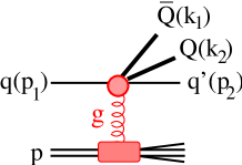
Figure 1: One gluon graph for heavy quark pair production by a quark in inelastic collision

In what follows we use the following notation (see Fig. 1): $p_{1,2}$ are the 4-momenta of the projectile quark q and the ejected quark $q^{\prime}$ respectively; $k_{1,2}$ are the 4-momenta of the produced heavy quarks $\bar{Q}$ and $Q$ respectively. For momenta combinations: $k=k_{1}+k_{2}$; $\alpha=k^{+}/p_{1}^{+}$; $\beta=k^{+}_{1}/k^{+}$; $M^{2}=(k_{1}+k_{2})^{2}$; $Q^{2}=-(p_{1}-p_{2})^{2}>0$; $\vec{\pi}=\alpha\vec{p}_{2}-(1-\alpha)\vec{k}$ is the relative transverse momentum between $q^{\prime}$ and $(\bar{Q}Q)$; $\vec{\kappa}=(1-\beta)\vec{k}_{1}-\beta\vec{k}_{2}$ is the relative transverse momentum between the heavy quarks.

To make further progress we switch from transverse momenta to impact parameters, which require further definitions: $\vec{r},\ \vec{r}_{1},\ \vec{r}_{2}$ are the transverse separations within the $\bar{Q}-Q$, $q-\bar{Q}$ and $q-Q$ pairs respectively; $\vec{\rho}=\vec{r}-\beta\vec{r}_{1}-(1-\beta)\vec{r}_{2}$ is the distance between $q^{\prime}$ and the center of gravity of the $\bar{Q}Q$ pair; $\vec{s}=\vec{r}_{1}-\vec{r}_{2}$ is the $\bar{Q}Q$ transverse separation.

Since we are interested in $\bar{Q}Q$ production in the projectile fragmentation region, the rapidity interval between the $q^{\prime}$ and $\bar{Q}Q$ is assumed to be short. At the same time the rapidity interval between the $\bar{Q}Q$ and the target is long (at high energies) and is filled by radiated gluons. The bottom blob in the graph in Fig. 1 includes all those gluons, while the upper part of the graph can be calculated using the Born approximation which is rather accurate for the projectile fragmentation region. This part is represented by the Born graphs depicted in Fig. 2.

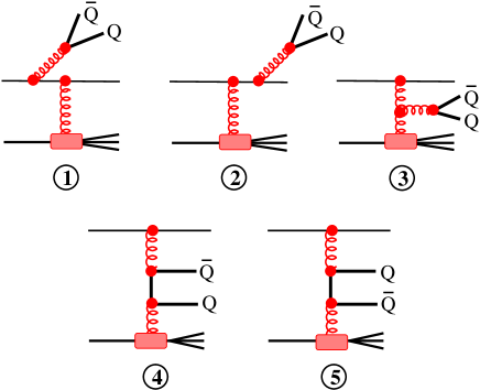
Figure 2: Feynman graphs contributing to inclusive production of a heavy quark pair.

The sum of this five amplitudes can be splited into two classes which we assign to bremsstrahlung (Br) and production (Pr) mechanisms, as is described in detail in Appendix A,

$$\sum\limits_{i=1}^{5}M^{T(L)}_{i}=M^{T(L)}_{Br}+M^{T(L)}_{Pr}\ ,$$ (7)

where the upper indexes $T$ and $L$ correspond to transverse or longitudinal polarization of the virtual gluon radiated by the projectile quark.

The transverse bremsstrahlung amplitude, $M^{T}_{Br}$, corresponds to the following combination of graphs depicted in Fig. 2 (see Appendix A.1),

$$M^{T}_{Br}=M^{T}_{1}+M^{T}_{2}+\frac{Q^{2}}{M^{2}+Q^{2}}\,M^{T}_{3}\ .$$ (8)

It describes bremsstrahlung of a transversely polarized heavy gluon which dissociates into $\bar{Q}Q$. The remaining transverse amplitudes are combined into the second group, the amplitude of $\bar{Q}Q$ production via direct interaction with the heavy quark pair,

$$M^{T}_{Pr}=\frac{M^{2}}{M^{2}+Q^{2}}\,M^{T}_{3}+M^{T}_{4}+M^{T}_{5}\ .$$ (9)

The procedure of grouping the longitudinal amplitudes is more complicated and is described in Appendix A.2. It leads also to the structure Eq. (7), where the bremsstrahlung and production longitudinal amplitudes are defined in (A.21).

Thus, the inclusive cross section has the following structure,

$$\frac{d\sigma(qp\to\bar{Q}QX)}{d\alpha\,d\beta}=\frac{d\sigma^{T}}{d\alpha\,d\beta}+\frac{d\sigma^{L}}{d\alpha\,d\beta}\ ,$$ (10)

where

$$\frac{d\sigma^{T(L)}(qp\to\bar{Q}QX)}{d\alpha\,d\beta}=\frac{d\sigma^{T(L)}_{Br}}{d\alpha\,d\beta}+\frac{d\sigma^{T(L)}_{Pr}}{d\alpha\,d\beta}+\frac{d\sigma^{T(L)}_{Int}}{d\alpha\,d\beta}\ .$$ (11)

The last term here corresponds to the interference of the amplitudes $M_{Br}$ and $M_{Pr}$.

II.1 Bremsstrahlung mechanism

The first term in the cross section Eq. (11) can be calculated in the framework of the light-cone dipole approach as follows,

$$\frac{d\sigma_{Br}(qp\to\bar{Q}QX)}{d\alpha\,d\beta}=\int\frac{d^{2}\kappa}{(2\pi)^{2}}\,d^{2}\rho\left|\Phi_{Br}(\vec{\rho},\vec{\kappa})\right|^{2}\Sigma_{1}(\vec{\rho});$$ (12)

Since the effective dipole cross section $\Sigma_{1}(\vec{\rho})$ is a function of one variable, for the sake of convenience we use here the light-cone distribution amplitudes in mixed impact parameter - transverse momentum representation,

$$\Phi_{Br}(\vec{\rho},\vec{\kappa})=\sum\limits_{\lambda}\Psi_{1}^{\lambda}(\vec{\rho})\Psi_{2}^{\lambda}(\vec{\kappa})+\Psi_{1}^{L}(\vec{\rho})\Psi_{2}^{L}(\vec{\kappa})\ ,$$ (13)

where the sum is over the transverse polarizations $\lambda$ of the radiated virtual gluon; the amplitude of longitudinal gluon radiation is labeled by the index $L$. Further notation is,

$$\Psi_{1}^{\lambda}(\vec{\rho}) = \frac{\sqrt{\alpha_{s}(1/\rho)}}{2\pi}\,\chi_{f}^{\dagger}\left\{i(2-\alpha)\vec{e}_{\lambda}\cdot\vec{\nabla}+\alpha\left[\vec{\sigma}\times\vec{e}_{\lambda}\right]\cdot\vec{\nabla}\right.$$ (14)

$$+ \left.i\alpha^{2}m_{q}\left[\vec{\sigma}\times\vec{e}_{\lambda}\right]\cdot\vec{n}\right\}\chi_{in}\,K_{0}(\tau\rho)\ ;$$

$$\Psi_{1}^{L}(\vec{\rho})=\frac{\sqrt{\alpha_{s}(1/\rho)}}{2\pi}\,\chi_{f}^{\dagger}\,2(1-\alpha)M\,\chi_{in}\,K_{0}(\tau\rho)\ ,$$ (15)

which are the light-cone distribution amplitudes for the quark-gluon Fock state with transversely polarized gluon (polarization $\lambda$) and longitudinal gluon respectively. The spinors $\chi_{in}$ and $\chi_{f}$ correspond to the initial and final light quarks. The running QCD coupling $\alpha_{s}(1/\rho)$ is taken at virtuality $\sim 1/\rho^{2}$.

The distribution amplitudes for a $\bar{Q}Q$ fluctuations of transversely and longitudinally polarized gluons respectively, read,

$$\Psi_{2}^{\lambda}(\vec{\kappa}) = \phi^{\dagger}\Bigl{\{}m_{q}\vec{\sigma}\cdot\vec{e}_{\lambda}+(1-2\beta)(\vec{\sigma}\cdot\vec{n})(\vec{e}_{\lambda}\cdot\vec{\kappa})$$ (16)

$$+ i\left[\vec{e}_{\lambda}\times\vec{n}\right]\cdot\vec{\kappa}\Bigr{\}}\,\bar{\phi}\,\frac{\alpha_{s}(\kappa)}{m_{Q}^{2}+\kappa^{2}}\ ;$$

$$\Psi_{2}^{L}(\vec{\kappa})=\phi^{\dagger}\,2\beta(1-\beta)M\vec{\sigma}\cdot\vec{n}\,\bar{\phi}\,\frac{\alpha_{s}(\kappa)}{m_{Q}^{2}+\kappa^{2}}\ ,$$ (17)

where $\phi$, $\bar{\phi}$ are the spinors of the heavy $Q$ and $\bar{Q}$ respectively;

$$\tau^{2} = (1-\alpha)M^{2}+\alpha^{2}m_{q}^{2}\ ;$$

$$M^{2} = \frac{m_{Q}^{2}+\kappa^{2}}{\beta(1-\beta)}\ ;$$

$m_{q}$ and $m_{Q}$ are the light and heavy quark masses respectively; $\vec{e}_{\lambda}$ is the polarization vector of the transverse gluon; $\vec{n}$ is the unit vector aligned along the direction of the projectile quark; $\vec{\sigma}$ are the Pauli matrices.

The dipole cross section $\Sigma_{1}(\rho)$ in (12) corresponds to gluon radiation by a quark hir ; kst1 ; kst2 . It has the form of the cross section for a gluon-quark-antiquark colorless system with transverse separations $\vec{\rho}$ for gluon-quark, $(1-\alpha)\vec{\rho}$ for gluon-antiquark, and $\alpha\vec{\rho}$ for quark-antiquark,

$$\Sigma_{1}(\vec{\rho})={9\over 8}\left\{\sigma(\vec{\rho})+\sigma\left[(1-\alpha)\vec{\rho}\right]\right\}-{1\over 8}\,\sigma(\alpha\vec{\rho})\ ,$$ (18)

where $\sigma(\rho)$ is the cross section of interaction of a $\bar{q}q$ dipole with transverse separation $\vec{\rho}$ on a proton.

II.2 Production mechanism

The second term in (11) is represented in a form similar to (12),

$$\frac{d\sigma_{Pr}(qp\to\bar{Q}QX)}{d\alpha\,d\beta}=\int\frac{d^{2}p_{2}}{(2\pi)^{2}}\,d^{2}s\left|\Phi_{Pr}(\vec{s},\vec{p}_{2})\right|^{2}\Sigma_{2}(\vec{s}),$$ (19)

with distribution amplitudes having structures similar to (12)-(17),

$$\Phi_{Pr}(\vec{s},\vec{p}_{2})=\sum\limits_{\bar{\lambda}}\Psi_{3}^{\bar{\lambda}}(\vec{s})\Psi_{4}^{\bar{\lambda}}(\vec{p}_{2})+\Psi_{3}^{L}(\vec{s})\Psi_{4}^{L}(\vec{p}_{2})\ ,$$ (20)

where

$$\Psi_{3}^{\bar{\lambda}}(\vec{s}) = \phi^{\dagger}\left\{m_{Q}\vec{\sigma}\cdot\vec{e}_{\bar{\lambda}}-i(1-2\beta)(\vec{\sigma}\cdot\vec{n})(\vec{e}_{\bar{\lambda}}\cdot\vec{\nabla})\right.$$ (21)

$$+ \left.\left[\vec{e}_{\bar{\lambda}}\times\vec{n}\right]\cdot\vec{\nabla}\right\}\,\bar{\phi}\,K_{0}(\epsilon s)\ ;$$

$$\Psi_{3}^{L}(\vec{s})=\phi^{\dagger}\,2\beta(1-\beta)Q\,\bar{\phi}\,K_{0}(\epsilon s)\ ,$$ (22)

are the light-cone $\bar{Q}Q$ distribution amplitudes in impact parameter representation. In the above expressions,

$$\epsilon^{2} = \beta(1-\beta)Q^{2}+m_{Q}^{2}\ ;$$

$$Q^{2} = \frac{\vec{p}_{2}^{\,2}+\alpha^{2}m_{q}^{2}}{1-\alpha}\ .$$ (23)

Notice that differently from the bremsstrahlung amplitudes, here the gluon virtuality $Q$ is not equal to the effective mass of the $\bar{Q}Q$.

Correspondingly, the transverse and longitudinal distribution amplitudes for quark-gluon fluctuation in momentum representation read,

$$\Psi_{4}^{\bar{\lambda}}(\vec{\kappa}) = \chi_{f}^{\dagger}\left\{(2-\alpha)\,\left(\vec{e}_{\bar{\lambda}}\cdot\vec{p}_{2}\right)+i\alpha\left[\vec{\sigma}\times\vec{e}_{\bar{\lambda}}\right]\cdot\vec{p}_{2}\right.$$ (24)

$$+ \left.i\alpha^{2}m_{2}\left[\vec{\sigma}\times\vec{e}_{\bar{\lambda}}\right]\cdot\vec{n}\right\}\,\bar{\chi}_{in}\,\frac{1}{\alpha^{2}m_{q}^{2}+p_{2}^{2}}\ ;$$

$$\Psi_{4}^{L}(\vec{p}_{2})=2(1-\alpha)\,\frac{\chi_{f}^{\dagger}\,Q\chi_{in}}{\alpha^{2}m_{q}^{2}+p_{2}^{2}}\ .$$ (25)

The dipole cross section $\Sigma_{2}(\vec{s})$ in (19) corresponds to gluon decay into a quark-antiquark pair hir ; kt-charm . Similar to (18) it also has the form of a cross section for a gluon-quark-antiquark colorless system, but with transverse separations $\vec{s}$ for the quark-antiquark, $\beta\vec{\rho}$ and $(1-\beta)\vec{\rho}$ for gluon-quark and gluon-antiquark, respectively.

$$\Sigma_{2}(\vec{s})={9\over 8}\left\{\sigma(\beta\vec{s})+\sigma\left[(1-\beta)\vec{s}\right]\right\}-{1\over 8}\,\sigma(\vec{s})\ .$$ (26)

II.3 Bremsstrahlung-Production interference

The third interference term in (11) reads,

$$\frac{d\sigma_{Int}(qp\to\bar{Q}QX)}{d\alpha\,d\beta}=2{\rm Re}\int d^{2}\rho\,d^{2}s$$ (27)

$$\times \left\langle\Phi^{\dagger}_{Pr}(\vec{\rho},\vec{s})\,\Phi_{Br}(\vec{\rho},\vec{s})\right\rangle\,\Sigma_{Int}(\vec{\rho},\vec{s}).$$

In this case the effective dipole cross section is function of two coordinates,

$$\Sigma_{Int}(\vec{\rho},\vec{s}) = {7\over 8}\Bigl{\{}\tilde{\sigma}(\vec{\rho},-\beta\vec{s})+\tilde{\sigma}\bigl{[}(1-\alpha)\vec{\rho},(1-\beta)\vec{s}\bigr{]}$$ (28)

$$- \tilde{\sigma}\bigl{[}\vec{\rho},(1-\beta)\vec{s}\bigr{]}\Bigr{\}}-{1\over 4}\Bigl{\{}\tilde{\sigma}\bigl{[}\vec{\rho},(1-\beta)\vec{s}\bigr{]}$$

$$+ \tilde{\sigma}\bigl{[}(1-\alpha)\vec{\rho},-\beta\vec{s}\bigr{]}-\tilde{\sigma}(\vec{\rho},-\beta\vec{s})\Bigr{\}}\ ,$$

where

$$\tilde{\sigma}(\vec{\rho},\vec{s})=\sigma(\vec{\rho}+\vec{s})-\sigma(\vec{\rho})-\sigma(\vec{s})\ .$$ (29)

For this reason we use in (27) the distribution functions $\Phi$ fully in impact parameter representation. They are related to the mixed representation functions given in Eqs. (13) and (20) as,

$$\Phi^{T(L)}_{Br}(\vec{\rho},\vec{s}) = \frac{1}{(2\pi)^{2}}\int d^{2}\kappa\,e^{-i\vec{\kappa}\cdot\vec{s}}\,\Phi^{T(L)}_{Br}(\vec{\rho},\vec{\kappa})\ ;$$ (30)

$$\Phi^{T(L)}_{Pr}(\vec{\rho},\vec{s}) = \frac{1}{(2\pi)^{2}}\int d^{2}p_{2}\,e^{-i\vec{p}_{2}\cdot\vec{s}}\,\Phi^{T(L)}_{Pr}(\vec{\rho},\vec{p}_{2})\ ;$$ (31)

This interference term, Eq. (27), turns out to be suppressed in the cross section compared to the first two terms in (11). Indeed, performing the integrations in Eqs. (12) and (19), one arrives at cross sections which expose the leading twist scale dependence both for the bremsstrahlung and production mechanisms,

$$\frac{d\sigma_{Br}}{d\alpha\,d\beta}\sim\frac{d\sigma_{Pr}}{d\alpha\,d\beta}\sim\frac{1}{m_{Q}^{2}}\ .$$ (32)

Indeed, the mean transverse separations squared, which are controlled by the distribution amplitudes Eqs. (14), (15) and Eqs. (21), (22), are $\langle\rho^{2}\rangle\sim 1/\epsilon^{2}\sim 1/m_{Q}^{2}$ and $\langle s^{2}\rangle\sim 1/\tau^{2}\sim 1/m_{Q}^{2}$, respectively. At such small separations the cross sections Eqs. (18) and (26) behave in accordance with color transparency zkl , $\Sigma_{1}(\vec{\rho})\propto\rho^{2}$ and $\Sigma_{2}(\vec{s})\propto s^{2}$, confirming (32). This result could be expected, since it also follows from the QCD factorization scheme.

As for the interference term, it follows from Eqs. (13) and (20) that the product of distribution amplitudes in (27), $\left\langle\Phi^{\dagger}_{Pr}(\vec{\rho},\vec{s})\,\Phi_{Br}(\vec{\rho},\vec{s})\right\rangle$, contains only coordinates squared, $\vec{\rho}^{\,2}$ and $\vec{s}^{\,2}$, but not their product, $\vec{\rho}\cdot\vec{s}$. At the same time, since the dipole cross section at small separation behaves as $\sigma(r)=C\,r^{2}$, the combination of cross sections, Eq. (29), reads,

$$\tilde{\sigma}(\vec{\rho},\vec{s})=2C\,\vec{\rho}\cdot\vec{s}\ .$$ (33)

Thus, the interference term Eq. (23) vanishes after integration over azimuthal angle.

In a more realistic model with a dipole cross section leveling off at large separations, Eq. (71). the result is not zero, but is a higher twist effect,

$$\frac{d\sigma_{Int}}{d\alpha\,d\beta}\sim\frac{1}{m_{Q}^{4}R^{2}_{0}(x)}\ ,$$ (34)

where $R_{0}(x)$ is defined in (71). Thus, the interference term in the cross section of inclusive heavy flavor production is vanishingly small. This observation turns out to be valid for diffractive production as well. Therefore, we safely neglect the interference in what follows.

III Diffractive production of heavy flavors in quark-proton collisions

Here we calculate the cross section of diffractive excitation of a projectile quark resulting in the production of a heavy quark pair,

$$q+p\to q\,\bar{Q}Q+p\ ,$$ (35)

as is shown in Fig. 3.

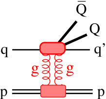
Figure 3: Diffractive production of a heavy quark pair in a quark-proton collision

This picture represents numerous Feynman graphs which are equivalent to a rather simple factorized form of the diffractive amplitude in the light-cone dipole representation. This formalism was developed for diffractive gluon bremsstrahlung in kst2 .

Similar to (8)-(9), the diffractive amplitude $A^{qp}$ can be splited into two parts,

$$A^{qp}=A_{Br}^{qp}+A_{Pr}^{qp}\ ,$$ (36)

where the bremsstrahlung and production amplitudes are defined as follows.

III.1 Bremsstrahlung mechanism of diffraction

The bremsstrahlung amplitude in (36) has the form,

$$A^{qp}_{Br}(\vec{\pi},\vec{\kappa})=\frac{3i}{16\pi}\int d^{2}\rho\,d^{2}s\,e^{i\vec{\pi}\cdot\vec{\rho}+i\vec{\kappa}\cdot\vec{s}}\,\Phi_{Br}(\vec{\rho},\vec{s})\,\tilde{\Sigma}_{1}(\vec{\rho},\vec{s})\ .$$ (37)

The distribution amplitude $\Phi_{Br}(\vec{\rho},\vec{s})$ in coordinate space is given by Eq. 30),

$$\Phi_{Br}(\vec{\rho},\vec{s}) = \Phi^{L}_{Br}(\vec{\rho},\vec{s})+\Phi^{T}_{Br}(\vec{\rho},\vec{s})=\frac{\sqrt{\alpha_{s}(1/s)\alpha_{s}(1/\rho)}}{(2\pi)^{2}}$$ (38)

$$\times \Bigl{[}4(1-\alpha)\frac{m_{Q}}{x}K_{1}(m_{Q}x)\chi_{f}\chi_{in}\phi^{\dagger}\vec{\sigma}\vec{n}\phi$$

$$+ \sum\limits_{\lambda}a_{\lambda}(\vec{\rho})\,b_{\lambda}(\vec{\nabla}_{s})\,\frac{1}{\rho^{2}}\,K_{0}(m_{Q}x)\Bigr{]}\ ,$$

where

$$a_{\lambda}(\vec{\rho})=\chi_{f}\Bigl{\{}i(2-\alpha)\vec{e}_{\lambda}\cdot\vec{\rho}+\alpha[\vec{\sigma}\times\vec{e}_{\lambda}]\cdot\vec{\rho}\Bigr{\}}\chi_{in};$$ (39)

$$b_{\lambda}(\vec{\nabla}_{s}) = \phi\Bigl{\{}m_{q}\vec{\sigma}\cdot\vec{e}_{\lambda}+[\vec{e}_{\lambda}\times\vec{n}]\cdot\vec{\nabla}_{s}$$ (40)

$$- i(1-2\beta)(\vec{\sigma}\cdot n)(\vec{e}_{\lambda}\cdot\nabla_{s})\Bigr{\}}\bar{\phi};$$

$$x = \sqrt{s^{2}+\frac{(1-\alpha)\rho^{2}}{\beta(1-\beta)}}\ .$$ (41)

The imaginary part of the amplitude of diffractive production of heavy flavors is calculated employing the generalized optical theorem (Cutkosky cutting rules) cutkosky . It is illustrated in Fig. 4 for the example of the bremsstrahlung mechanism, and is used in the same way for other mechanisms in what follows.

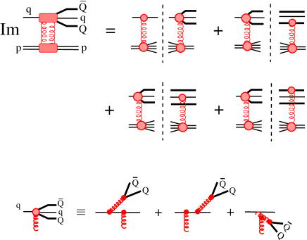
Figure 4: Cutkosky rules for the imaginary part of the amplitude of diffractive $\bar{Q}Q$ production in quark-proton collision. Only bremsstrahlung mechanism is considered for this example.

The amplitudes shown in the graphs on both sides of the unitarity cut (vertical dashed line) are on-mass-shell physical processes, and the final state excitations of the proton are summed up employing completeness. After integration over impact parameter $\vec{b}$, this procedure leads to the following form for the effective cross section $\tilde{\Sigma}_{1}$ in (37),

$$\tilde{\Sigma}_{1}(\vec{\rho},\vec{s})=\left({1\over 9}+{5\over 24}\,\tau^{q}_{a}\tau^{Q}_{a}\right)\Bigl{\{}\sigma\left[\vec{\rho}-(1-\beta)\vec{s}\right]$$ (42)

$$- \sigma\left[\vec{\rho}+\beta\vec{s}\right]-\sigma\left[(1-\alpha)\vec{\rho}-(1-\beta)\vec{s}\right]$$

$$+ \sigma\left[(1-\alpha)\vec{\rho}+\beta\vec{s}\right]\Bigr{\}}+{3\over 4}\,\tau^{q}_{a}\tau^{Q}_{a}\Bigl{\{}\sigma[\vec{\rho}]-\sigma[(1-\alpha)\vec{\rho}]$$

$$+ \sigma[(1-\beta)\vec{s}]-{1\over 2}\,\sigma[(1-\alpha)\vec{\rho}-(1-\beta)\vec{s}]$$

$$- {1\over 2}\,\sigma[\vec{\rho}-(1-\beta)\vec{s}]-\sigma[\beta\vec{s}]$$

$$+ {1\over 2}\,\sigma[(1-\alpha)\vec{\rho}-\beta\vec{s}]+{1\over 2}\,\sigma[\vec{\rho}+\beta\vec{s}]\Bigr{\}}\ .$$

Here $\tau^{q}_{a}={1\over 2}\lambda^{q}_{a}$ and $\tau^{Q}_{a}={1\over 2}\lambda^{Q}_{a}$, where $\lambda^{q}_{a}$ and $\lambda^{Q}_{a}$ are the Gell-Mann matrices acting on the color spaces of light and heavy quarks respectively.

The corresponding bremsstrahlung term in the diffractive cross section reads,

$$\left.\frac{d\sigma_{Br}(qp\to\bar{Q}Qqp)}{dt^{\prime}\,d\alpha\,d\beta}\right|_{t^{\prime}=0}=\frac{3}{256\pi}\int d^{2}\rho\,d^{2}s$$ (43)

$$\times \left|\Phi_{Br}(\vec{\rho},\vec{s})\right|^{2}\,{\rm Tr}_{q}{\rm Tr}_{Q}\left[\tilde{\Sigma}_{1}(\vec{\rho},\vec{s})\tilde{\Sigma}_{1}^{\dagger}(\vec{\rho},\vec{s})\right]\ ,$$

where the traces Tr_q and Tr_Q are taken over the Gell-Mann matrices corresponding to light and heavy quarks respectively.

III.2 Production mechanism of diffraction

The production term in (36) reads,

$$A^{qp}_{Pr}=\frac{3i}{16\pi}\int d^{2}\rho\,d^{2}s\,e^{i\vec{\pi}\cdot\vec{\rho}+i\vec{\kappa}\cdot\vec{s}}\,\Phi_{Pr}(\vec{\rho},\vec{s})\,\tilde{\Sigma}_{2}(\vec{\rho},\vec{s})\ ,$$ (44)

where

$$\Phi_{Pr}(\vec{\rho},\vec{s})=\Phi^{L}_{Pr}(\vec{\rho},\vec{s})+\Phi^{T}_{Pr}(\vec{\rho},\vec{s})=\frac{\sqrt{\alpha_{s}(1/s)\alpha_{s}(1/\rho)}}{(2\pi)^{2}}$$ (45)

$$\times \Bigl{\{}4(1-\alpha)\frac{m_{Q}}{x}K_{1}(m_{Q}x)\chi_{f}\chi_{in}\phi^{\dagger}\vec{\sigma}\vec{n}\phi$$

$$+ \sum\limits_{\lambda}a_{\lambda}(\vec{\rho})\,b_{\lambda}(\vec{\nabla}_{s})\,\frac{1}{\rho^{2}}\bigl{[}K_{0}(m_{Q}s)-K_{0}(m_{Q}x)\Bigr{\}}\ ,$$

The functions $a_{\lambda}(\vec{\rho})$, $b_{\lambda}(\vec{\nabla}_{s})$ and $x$ are defined in (39)-(41).

$$\tilde{\Sigma}_{2}(\vec{\rho},\vec{s})=\left({1\over 9}+{5\over 24}\,\tau^{q}_{a}\tau^{Q}_{a}\right)\Bigl{\{}\sigma\left[\vec{\rho}+\beta\vec{s}\right]$$ (46)

$$- \sigma\left[\vec{\rho}-(1-\beta)\vec{s}\right]+\sigma\left[(1-\alpha)\vec{\rho}+\beta\vec{s}\right]$$

$$- \sigma\left[(1-\alpha)\vec{\rho}-(1-\beta)\vec{s}\right]\Bigr{\}}+{7\over 12}\,\tau^{q}_{a}\tau^{Q}_{a}\sigma[\vec{s}]+$$

$$+ {3\over 4}\,\tau^{q}_{a}\tau^{Q}_{a}\Bigl{\{}\sigma[\vec{s}]-\sigma[(1-\beta)\vec{s}]-\sigma[\beta\vec{s}]+\sigma(\vec{\rho})$$

$$- \sigma[(1-\alpha)\vec{\rho}]+{1\over 2}\,\sigma[(1-\alpha)\vec{\rho}-(1-\beta)\vec{s}]$$

$$+ {1\over 2}\,\sigma[(1-\alpha)\vec{\rho}+\beta\vec{s}]-{1\over 2}\,\sigma[\vec{\rho}-(1-\beta)\vec{s}]$$

$$- {1\over 2}\,\sigma[\vec{\rho}+\beta\vec{s}]\Bigr{\}}\ .$$

Eventually we arrive at the production cross section,

$$\left.\frac{d\sigma_{Pr}(qp\to\bar{Q}Qqp)}{dt^{\prime}\,d\alpha\,d\beta}\right|_{t^{\prime}=0}=\frac{3}{256\pi}\int d^{2}\rho\,d^{2}s$$ (47)

$$\times \left|\Phi_{Pr}(\vec{\rho},\vec{s})\right|^{2}\,{\rm Tr}_{q}{\rm Tr}_{Q}\left[\tilde{\Sigma}_{2}(\vec{\rho},\vec{s})\tilde{\Sigma}_{2}^{\dagger}(\vec{\rho},\vec{s})\right]\ .$$

III.3 Scale dependence

In the bremsstrahlung distribution amplitude, Eq. (38), both mean separations are controlled by the hard scale,

$$\langle\rho^{2}\rangle\sim\langle s^{2}\rangle\sim\frac{1}{m_{Q}^{2}}\ .$$ (48)

Therefore, the corresponding term Eq. (43) in the diffractive cross section is as small as $1/m_{Q}^{4}$, i.e. it is a higher twist effect.

On the contrary, in the production mechanism only the $\bar{Q}Q$ separation is small, $\langle s^{2}\rangle\sim 1/m_{Q}^{2}$. The mean separation between the light quark $q^{\prime}$ and the $\bar{Q}Q$ according to (24)-(25) is large, $\langle\rho^{2}\rangle\sim 1/m_{q}^{2}$. However, the effective cross section Eq. (46) cannot be large. Indeed, at small $s\to 0$ it vanishes as

$$\tilde{\Sigma}_{2}(\vec{\rho},\vec{s})\propto\vec{s}\cdot\vec{\rho}\ .$$ (49)

This result is similar to what was found in kpst-dy for the diffractive Drell-Yan reaction, which also probes simultaneously large and small distances. This is very nontrivial, since in the case of the Drell-Yan reaction that property is due to the Abelian nature of the radiated particle. Now we have a non-Abelian radiation, but arrived at the same feature.

It is interesting to notice that while the forward Abelian radiation by a quark is forbidden, the bremsstrahlung part of the diffractive radiation of a $\bar{Q}Q$ pair, although is not zero, turns out to be quite suppressed.

For further calculations we can safely neglect the higher twist contribution of the bremsstrahlung mechanism to the quark-proton diffractive amplitude, and keep only the leading twist production term, Eq. (47).

IV Diffractive production of heavy flavors by a gluon

Not only quarks, but projectile gluons can also be diffractively excited producing a heavy $\bar{Q}Q$ pair, as is illustrated in Fig. 5.

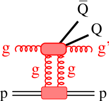
Figure 5: Diffractive production of a heavy quark pair in a gluon-proton collision

This contribution is important if the $\bar{Q}Q$ pair carries a small fraction of the initial beam momentum.

The calculations are similar to those that we performed in Sect. III.2. Here we neglect the higher twist bremsstrahlung contribution. The leading twist amplitude of diffractive $\bar{Q}Q$ pair production by a projectile gluon, $g+p\to\bar{Q}QX+p$, reads,

$$A^{(Gp)}_{Pr}=\frac{3i}{16\pi}\int d^{2}\rho\,d^{2}s\,e^{i\vec{\pi}\cdot\vec{\rho}+i\vec{\kappa}\cdot\vec{s}}\,\Phi^{(Gp)}_{Pr}(\vec{\rho},\vec{s})\,\tilde{\Sigma}_{3}(\vec{\rho},\vec{s})\ ,$$ (50)

where

$$\Phi^{(Gp)}_{Pr}(\vec{\rho},\vec{s}) = \frac{\sqrt{\alpha_{s}(1/\rho)\alpha_{s}(1/s)}}{(2\pi)^{2}}\,\Bigl{\{}4\frac{m_{Q}}{x}\,K_{1}(m_{Q}x)\,\vec{e}_{f}\cdot\vec{e}_{in}$$

$$+ \sum\limits_{\lambda}a_{\lambda}(\vec{\rho})b_{\lambda}(\vec{\nabla}_{s})\frac{1}{\rho^{2}}\bigl{[}K_{0}(m_{Q}s)-K_{0}(m_{Q}x)\bigr{]}\Bigr{\}}$$

Here

$$a_{\lambda}(\vec{\rho}) = 2i\bigl{[}(1-\alpha)(\vec{e}_{f}\cdot\vec{e}_{in})(\vec{e}_{\lambda}\cdot\vec{\rho})+\alpha(\vec{e}_{in}\cdot\vec{e}_{\lambda})(\vec{e}_{f}\cdot\vec{\rho})$$ (52)

$$- \alpha(\vec{e}_{f}\cdot\vec{e}_{\lambda})(\vec{e}_{i}\cdot\vec{\rho})\bigr{]}\ ,$$

$b_{\lambda}(\vec{\nabla}_{s})$ is given by Eq. (40), $x$ is given by (41), $\vec{e}_{in}$ and $\vec{e}_{f}$ are the polarization vectors of gluons in the initial and final states respectively, and $\vec{e}_{\lambda}$ is the transverse polarization vector of the virtual $t$-channel gluon. The first and the second terms in the r.h.s. of Eq. (LABEL:314) correspond to exchange in the $t$-channel of longitudinally and transversely polarized gluons respectively.

The effective cross section in (50) is given by

$$\tilde{\Sigma}_{3}(\vec{\rho},\vec{s}) = \left({1\over 4}\delta_{ab}+{3\over 8}d_{abc}\tau_{c}\right)\Bigl{\{}\sigma\bigl{[}(1-\alpha)\vec{\rho}-(1-\beta)\vec{s}\bigr{]}$$ (53)

$$+ \sigma\bigl{[}\vec{\rho}-(1-\beta)\vec{s}\bigr{]}-\sigma\bigl{[}(1-\alpha)\vec{\rho}+\beta\vec{s}\bigr{]}$$

$$- \sigma\bigl{[}\vec{\rho}+\beta\vec{s}\bigr{]}\Bigr{\}}+\frac{3i}{8}\,f_{abd}\tau_{d}\Bigl{\{}2\sigma\bigl{[}(1-\alpha)\rho\bigr{]}$$

$$- \sigma\bigl{[}(1-\alpha)\vec{\rho}+\beta\vec{s}\bigr{]}-\sigma\bigl{[}(1-\alpha)\vec{\rho}-(1-\beta)\vec{s}\bigr{]}$$

$$- 2\sigma(\rho)+\sigma\bigl{[}\vec{\rho}+\beta\vec{s}\bigr{]}+\sigma\bigl{[}\vec{\rho}-(1-\beta)\vec{s}\bigr{]}$$

$$- 2\sigma(\beta s)-2\sigma\bigl{[}(1-\beta)s\bigr{]}+{32\over 9}\sigma(s)\Bigr{\}}\,.$$

The indexes $a,\ b$ correspond to the initial and final state polarizations of the gluons, and $d_{abc}$ and $f_{abc}$ are the structure constants.

Eventually, the differential cross section of diffractive production of a $\bar{Q}Q$ pair in gluon-proton collision by the production mechanism (leading twist) turns out to be

$$\left.\frac{d\sigma_{Pr}(Gp\to G\bar{Q}Qp)}{dt^{\prime}\,d\alpha\,d\beta}\right|_{t^{\prime}=0}$$

$$= \frac{9}{256\pi}\int d^{2}\rho d^{2}s\left|\Phi^{(Gp)}_{Pr}(\vec{\rho},\vec{s})\right|^{2}{\rm Tr}_{Q}\left\langle\tilde{\Sigma}_{3}(\vec{\rho},\vec{s})\tilde{\Sigma}_{3}^{\dagger}(\vec{\rho},\vec{s})\right\rangle$$

Here the brackets $\bigl{\langle}...\bigr{\rangle}$ indicate the averaging over initial and summing over final color indexes of the gluons.

V Diffractive proton-proton collisions

Now we consider a large rapidity gap single diffractive process,

$$p+p\to\bar{Q}QX+p\,,$$ (55)

where one colliding proton remains intact, and the debris of the other proton contains a heavy $\bar{Q}Q$ pair. Similar to the quark-proton collision, the amplitude of this reaction can be splited into bremsstrahlung and production parts,

$$A^{pp}=A^{pp}_{Br}+A^{pp}_{Pr}\ ,$$ (56)

which are described below.

V.1 Leading twist bremsstrahlung contribution

The first bremsstrahlung term in (56) is represented by graphs depicted in Fig. 6.

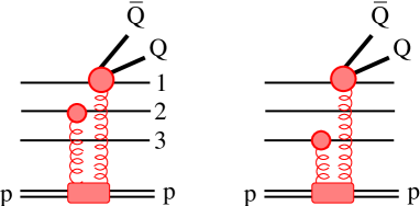
Figure 6: Diffractive production of a heavy quark pair in a proton-proton collision. More graphs emerge after quark permutation.

We neglect the higher twist term corresponding to attachment of both t-channel gluons to the same valence quark in the projectile proton. More diagrams are generated by permutation of the projectile quarks.

The diffractive amplitude corresponding to the graphs in Fig. 6 has the form,

$$A_{Br}^{pp} = \frac{3i}{16\pi}\int d^{2}\rho\,d^{2}s\,\prod\limits_{i=1}^{3}d^{2}r_{i}\,dx_{i}\,e^{i\vec{\pi}\cdot\vec{\rho}+i\vec{\kappa}\cdot\vec{s}}$$ (57)

$$\times \Psi_{f}^{\dagger}(\vec{r}_{1},\vec{r}_{2},\vec{r}_{3},x_{1},x_{2},x_{3})\,\Sigma^{pp}_{Br}(\vec{\rho},\vec{s},\vec{r}_{1},\vec{r}_{2},\vec{r}_{3})$$

$$\times \Phi_{Br}(\vec{\rho},\vec{s})\,\Psi_{in}^{\dagger}(\vec{r}_{1},\vec{r}_{2},\vec{r}_{3},x_{1},x_{2},x_{3}).$$

Here $\Psi_{in}$ is the light-cone wave function of the valence $|3q\rangle$ Fock component of the projectile proton, and $\Psi_{f}$ is the final state wave function of the recoil $|3q\rangle$ system after radiation of the $\bar{Q}Q$.

The effective dipole cross section has the following structure,

$$\Sigma_{Br}^{pp}(\vec{\rho},\vec{s},\vec{r}_{1},\vec{r}_{2},\vec{r}_{3})=$$ (58)

$$\left[{1\over 6}\,\delta_{ab}+{1\over 2}\,d_{abc}\tau^{q_{1}}_{c}\right]\,\tau^{Q}_{b}\left[\tau^{q_{2}}_{a}\sigma_{1}(\vec{r}_{12},\vec{\rho})+\tau^{q_{3}}_{a}\sigma_{1}(\vec{r}_{13},\vec{\rho})\right]$$

$$+ {i\over 2}\,f_{abc}\tau^{q_{1}}_{c}\tau^{Q}_{b}\left[\tau^{q_{2}}_{a}\sigma_{2}(\vec{r}_{12},\vec{\rho})+\tau^{q_{3}}_{a}\sigma_{2}(\vec{r}_{13},\vec{\rho})\right]$$

$$+ {\rm quark\ permutations}\ ,$$

where the upper index $q_{i}$ ($i=1,2,3$) indicates the active quarks.

The following new notation is introduced here,

$$\sigma_{1}(\vec{r},\vec{\rho}) = \sigma(\vec{r}+\alpha\vec{\rho})-\sigma(\vec{r})\ ,$$

$$\sigma_{2}(\vec{r},\vec{\rho}) = 2\sigma[\vec{r}-(1-\alpha)\vec{\rho}]-\sigma(\vec{r}+\alpha\vec{\rho})-\sigma(\vec{r})\ ,$$

$$\vec{r}_{12} = \vec{r}_{1}-\vec{r}_{2}\ ,\ \ \ \ \vec{r}_{13}=\vec{r}_{1}-\vec{r}_{3}\ .$$ (59)

The differential cross section corresponding to the amplitude Eq. (57) reads,

$$\frac{d\sigma_{Br}(pp\to\bar{Q}QXp)}{dt^{\prime}\,dz_{1}\,dz_{2}}=\int d^{2}\kappa\,d^{2}\pi\,\sum\limits_{f}\left|A_{Br}^{pp}\right|^{2}\ ,$$ (60)

One can employ completeness for the final state $|3q\rangle$ system,,

$$\sum\limits_{f}\Psi_{f}(\vec{r}_{1},\vec{r}_{2},\vec{r}_{3},x_{1},x_{2},x_{3})\Psi_{f}^{\dagger}(\vec{r}_{1}^{\,\prime},\vec{r}_{2}^{\,\prime},\vec{r}_{3}^{\,\prime},x_{1}^{\prime},x_{2}^{\prime},x_{3}^{\prime})$$ (61)

$$= \prod\limits_{i}^{3}\delta(\vec{r}_{i}-\vec{r}_{i}^{\,\prime})\,\delta(x_{i}-x_{i}^{\prime})\ .$$

Applying this condition to (60) and averaging over color indexes we get,

$$\frac{d\sigma_{Br}(pp\to\bar{Q}QXp)}{dt^{\prime}\,dz_{1}\,dz_{2}}=\frac{9}{256\pi}\int d^{2}\rho\,d^{2}s\prod\limits_{i}^{3}d^{2}r_{i}\,dx_{i}$$

$$\times \Bigl{|}\Psi_{in}(\vec{r}_{1},\vec{r}_{2},\vec{r}_{3},x_{1},x_{2},x_{3})\Bigr{|}^{2}\,\Bigl{|}\Phi_{Br}(\vec{\rho},\vec{s})\Bigr{|}^{2}$$

$$\times {\rm Tr}_{Q}\left\langle\Sigma^{pp}_{Br}(\vec{\rho},\vec{s},\vec{r}_{1},\vec{r}_{2},\vec{r}_{3})\left.\Sigma^{pp}_{Br}\right.^{\dagger}(\vec{\rho},\vec{s},\vec{r}_{1},\vec{r}_{2},\vec{r}_{3})\right\rangle\ .$$

Here the trace is performed only over color indexes of the $\bar{Q}Q$ pair, while the brackets indicate averaging over the colorless $|3q\rangle$ state in the proton. This trace results in,

$${\rm Tr}_{Q}\left\langle\Sigma^{pp}_{Br}(\vec{\rho},\vec{s},\vec{r}_{1},\vec{r}_{2},\vec{r}_{3})\left.\Sigma^{pp}_{Br}\right.^{\dagger}(\vec{\rho},\vec{s},\vec{r}_{1},\vec{r}_{2},\vec{r}_{3})\right\rangle$$ (63)

$$= {109\over 108}\,\sigma^{2}_{1}(\vec{r}_{12},\vec{\rho})+{1\over 4}\,\sigma^{2}_{2}(\vec{r}_{12},\vec{\rho})-{1\over 6}\,\sigma_{1}(\vec{r}_{12},\vec{\rho})\sigma_{2}(\vec{r}_{12},\vec{\rho})$$

$$+ {11\over 216}\,\sigma_{1}(\vec{r}_{12},\vec{\rho})\sigma_{1}(\vec{r}_{13},\vec{\rho})+{1\over 8}\,\sigma_{2}(\vec{r}_{12},\vec{\rho})\sigma_{2}(\vec{r}_{13},\vec{\rho})$$

$$- {5\over 14}\,\sigma_{1}(\vec{r}_{12},\vec{\rho})\sigma_{2}(\vec{r}_{13},\vec{\rho})$$

$$+ \{\vec{r}_{12}\rightleftharpoons\vec{r}_{13}\}+{\rm quark\ permutations}\ .$$

Further integrations in Eq. (LABEL:390) are straightforward.

V.2 Leading twist production mechanism

In this case the main contribution emerges from the diffractive interaction of a separate valence quark, although the interaction of spectators should be included as well. The full set of graphs having the leading twist behavior, $1/m_{Q}^{2}$, in the cross section is shown in Fig. 7).

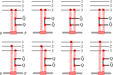
Figure 7: Diffractive production graphs providing $1/m_{Q}^{2}$ contribution to the cross section. The projectile valence quarks should be permuted.

In all these graphs two gluons are attached to the target and beam protons. The former is obvious, since we want to have a large rapidity gap and also that the recoil target proton remains intact. As for two gluons attached to the beam, this condition is due to the leading twist behavior we would like to have. Indeed, in the set of graph where only one gluon is attached to the projectile, the second $t$-channel gluon is probing the small sizes $r\sim 1/m_{Q}$ in the dissociation process $G\to\bar{Q}Q$. Thus one gains an additional suppression $1/m_{Q}^{2}$. i.e. a higher twist behavior. Notice, however, that the pairs of gluons attached to the target and the beam are not symmetric, the former are in a colorless state, while in the latter all colors are summed up.

The cross section corresponding to the graphs depicted in Fig. 7 has a form similar to (LABEL:390),

$$\frac{d\sigma_{Pr}(pp\to\bar{Q}QXp)}{dt^{\prime}\,dz_{1}\,dz_{2}}=\frac{9}{256\pi}\int d^{2}\rho\,d^{2}s\prod\limits_{i}^{3}d^{2}r_{i}\,dx_{i}$$

$$\times \Bigl{|}\Psi_{in}(\vec{r}_{1},\vec{r}_{2},\vec{r}_{3},x_{1},x_{2},x_{3})\Bigr{|}^{2}\,\Bigl{|}\Phi_{Pr}(\vec{\rho},\vec{s})\Bigr{|}^{2}$$

$$\times {\rm Tr}_{Q}\left\langle\Sigma^{pp}_{Pr}(\vec{\rho},\vec{s},\vec{r}_{1},\vec{r}_{2},\vec{r}_{3})\left.\Sigma^{pp}_{Pr}\right.^{\dagger}(\vec{\rho},\vec{s},\vec{r}_{1},\vec{r}_{2},\vec{r}_{3})\right\rangle\ .$$

In this case the effective dipole cross section has the form,

$$\Sigma^{pp}_{Pr}(\vec{\rho},\vec{s},\vec{r}_{1},\vec{r}_{2},\vec{r}_{3})=$$ (65)

$$(\tau^{q_{1}}_{a}\tau^{q_{1}}_{b})\,\left[(\tau^{Q}_{a}\tau^{Q}_{b})\,\sigma_{3}(\vec{\rho},\vec{s})+(\tau^{Q}_{b}\tau^{Q}_{a})\,\sigma_{4}(\vec{\rho},\vec{s})\right]$$

$$+ \tau^{q_{1}}_{a}(\tau^{Q}_{a}\tau^{Q}_{b})\Bigl{[}\tau^{q_{2}}_{b}\,\sigma_{5}(\vec{r}_{12},\vec{\rho},\vec{s})+\tau^{q_{3}}_{b}\,\sigma_{5}(\vec{r}_{13},\vec{\rho},\vec{s})$$

$$+ \tau^{q_{1}}_{a}(\tau^{Q}_{b}\tau^{Q}_{a})\Bigl{[}\tau^{q_{2}}_{b}\,\sigma_{6}(\vec{r}_{12},\vec{\rho},\vec{s})+\tau^{q_{3}}_{b}\,\sigma_{6}(\vec{r}_{13},\vec{\rho},\vec{s})\Bigr{]}\ ^{\prime}$$

$$+ {\rm quark\ permutations}\ .$$

where

$$\sigma_{3}(\vec{\rho},\vec{s}) = {1\over 2}\Bigl{\{}\sigma(\vec{\rho})-\sigma(\vec{\rho}-\beta\vec{s})-\sigma[(1-\alpha)\vec{\rho}]$$

$$+ \sigma[(1-\alpha)\vec{\rho}+(1-\beta)\vec{s}]\;\Bigr{\}}$$

$$\sigma_{4}(\vec{\rho},\vec{s}) = {1\over 2}\Bigl{\{}\sigma[\vec{\rho}+(1-\beta)\vec{s}]-\sigma(\vec{\rho})+\sigma[(1-\alpha)\vec{\rho}]$$

$$- \sigma[(1-\alpha)\vec{\rho}-\beta\vec{s}]\Bigr{\}}\ ;$$

$$\sigma_{5}(\vec{r}_{1i},\vec{\rho},\vec{s}) = \sigma[\vec{r}_{1i}-(1-\alpha)\vec{\rho}]$$

$$- \sigma[\vec{r}_{1i}-(1-\alpha)\vec{\rho}+\beta\vec{s}]\ ;$$

$$\sigma_{6}(\vec{r}_{1i},\vec{\rho},\vec{s}) = \sigma[\vec{r}_{1i}-(1-\alpha)\vec{\rho}-(1-\beta)\vec{s}]$$

$$- \sigma[\vec{r}_{1i}-(1-\alpha)\vec{\rho}]\ ,$$

$$i = 2,\ 3\ .$$ (66)

The trace of the product of the effective cross sections in (LABEL:410) has the form,

$${\rm Tr}_{Q}\left\langle\Sigma^{pp}_{Pr}(\vec{\rho},\vec{s},\vec{r}_{1},\vec{r}_{2},\vec{r}_{3})\left.\Sigma^{pp}_{Pr}\right.^{\dagger}(\vec{\rho},\vec{s},\vec{r}_{1},\vec{r}_{2},\vec{r}_{3})\right\rangle$$ (67)

$$= {19\over 6}\,\sigma_{3}^{2}(\vec{\rho},\vec{s})+{2\over 3}\,\sigma_{4}^{2}(\vec{\rho},\vec{s})-{2\over 3}\,\sigma_{3}(\vec{\rho},\vec{s})\,\sigma_{4}(\vec{\rho},\vec{s})$$

$$+ {1\over 9}\,\sigma_{4}(\vec{\rho},\vec{s})\left[\sigma_{5}(\vec{r}_{12},\vec{\rho},\vec{s})+\sigma_{5}(\vec{r}_{13},\vec{\rho},\vec{s})\right]$$

$$- {2\over 9}\,\sigma_{4}(\vec{\rho},\vec{s})\left[\sigma_{6}(\vec{r}_{12},\vec{\rho},\vec{s})+\sigma_{6}(\vec{r}_{13},\vec{\rho},\vec{s})\right]$$

$$- {19\over 18}\,\sigma_{3}(\vec{\rho},\vec{s})\left[\sigma_{5}(\vec{r}_{12},\vec{\rho},\vec{s})+\sigma_{5}(\vec{r}_{13},\vec{\rho},\vec{s})\right]$$

$$+ {1\over 9}\,\sigma_{3}(\vec{\rho},\vec{s})\left[\sigma_{6}(\vec{r}_{12},\vec{\rho},\vec{s})+\sigma_{6}(\vec{r}_{13},\vec{\rho},\vec{s})\right]$$

$$+ {1\over 9}\,\,\left[\sigma_{5}(\vec{r}_{12},\vec{\rho},\vec{s})\,\sigma_{6}(\vec{r}_{12},\vec{\rho},\vec{s})+\sigma_{5}(\vec{r}_{13},\vec{\rho},\vec{s})\,\sigma_{6}(\vec{r}_{13},\vec{\rho},\vec{s})\right]$$

$$+ {5\over 18}\,\left[\sigma_{5}^{2}(\vec{r}_{12},\vec{\rho},\vec{s})+\sigma_{5}^{2}(\vec{r}_{13},\vec{\rho},\vec{s})+\sigma_{6}^{2}(\vec{r}_{12},\vec{\rho},\vec{s})+\right.$$

$$+ \left.\sigma_{6}^{2}(\vec{r}_{13},\vec{\rho},\vec{s})\right]+{2\over 9}\,\sigma_{5}(\vec{r}_{12},\vec{\rho},\vec{s})\,\sigma_{5}(\vec{r}_{13},\vec{\rho},\vec{s})$$

$$- {1\over 3}\,\sigma_{6}(\vec{r}_{12},\vec{\rho},\vec{s})\,\sigma_{6}(\vec{r}_{13},\vec{\rho},\vec{s})-{1\over 6}\,\left[\sigma_{5}(\vec{r}_{12},\vec{\rho},\vec{s})\,\sigma_{6}(\vec{r}_{13},\vec{\rho},\vec{s})\right.$$

$$+ \left.\sigma_{5}(\vec{r}_{13},\vec{\rho},\vec{s})\,\sigma_{6}(\vec{r}_{12},\vec{\rho},\vec{s})\right]\ .$$

The dipole cross sections $\sigma_{k}$ ($k=3,4,5,6$) vanish linearly in $\vec{s}$ as $\vec{s}\to 0$. Since the mean value of $s$, controlled by the distribution function $\Psi_{Pr}(\vec{\rho},\vec{s})$, is small, $\langle\vec{s}^{\,2}\rangle\sim 1/m_{Q}^{2}$, one can make an expansion,

$$\sigma(\vec{r}+\vec{s}_{1,2})-\sigma(\vec{r})\approx\vec{s}_{1,2}\cdot\vec{\nabla}\,\sigma(\vec{r})\ ,$$ (68)

where $\vec{s}_{1}=\beta\vec{s}$, $\vec{s}_{2}=-(1-\beta)\vec{s}$, and $\vec{r}$ is one of the distances $\vec{\rho},\ \vec{r}_{ik}$, etc.

VI Saturation of unitarity and breakdown of QCD factorization

Factorization assumes that the hard interaction of partons and subsequent hadronization proceed independently of the soft spectator partons in the beam and target. This cannot be true for diffraction associated with a large rapidity gap (LRG). Indeed, the short range hard interaction of partons guarantees an overlap of the colliding hadrons, large impact parameters do not contribute. It is known from data that for such near central collisions unitarity is almost saturated k3p , i.e. the chance for colliding hadrons to escape without soft inelastic interactions which terminate the LRG is very small.

Here we rely on a simple eikonal model kps1 ; bkss ; kpst-dy . The absorptive corrections to the hard diffractive amplitude lead to a suppression factor,

$$A_{if}(b)\Rightarrow A_{if}(b)\,\left[1-{\rm Im}f^{pp}_{el}(b)\right]\ ,$$ (69)

where $f^{pp}_{el}(b)$ is the partial elastic amplitude. We assume a Gaussian shape for the elastic and diffraction amplitudes. After squaring the amplitude Eq. (69) and integrating over impact parameter we arrive at the following suppression factor for the diffractive cross section Eq. (LABEL:410),

$$K = \left\{1-{1\over{\pi}}\,\frac{\sigma^{pp}_{tot}(s)}{B_{sd}(s)+2B^{pp}_{el}(s)}\right.$$ (70)

$$+ \left.\frac{1}{(4\pi)^{2}}\,\frac{\left[\sigma^{pp}_{tot}(s)\right]^{2}}{B^{pp}_{el}(s)\left[B_{sd}(s)+B^{pp}_{el}(s)\right]}\right\}\ .$$

Here the elastic slope depends on energy as $B^{pp}_{el}(s)=B^{0}_{el}+2\,\alpha^{\prime}_{{\bf I\!P}}\,\ln(s/s_{0})$ with $B^{0}_{el}=7.5\,\mbox{GeV}^{-2}$, $s_{0}=1\,\mbox{GeV}^{2}$. The slope of single-diffractive hard cross section can be estimated as, $B_{sd}(s)\approx\langle r_{ch}^{2}\rangle/3+2\,\alpha^{\prime}_{{\bf I\!P}}$, where the proton mean charge radius squared is $\langle r_{ch}^{2}\rangle=0.8\,\mbox{fm}^{2}$.

A more accurate estimate needs a detailed information about the transverse structure of different Fock states. Such information is very much model dependent. Upon reaching the unitarity limit (Froissart bound) the fraction of diffractive events is expected to vanish as $1/\ln(s)$ brazil . How soon it may happen depends on specific models. For instance if gluons form dense spots inside hadrons, those spots can approach the unitarity limit much faster than the whole hadron-hadron scattering amplitude. Such black spots will suppress diffractive gluonic reactions (heavy flavors, triple-Pomeron term, etc.) much more than is suggested by Eq. (70). Therefore, the predicted energy dependence of the survival probability Eq. (70) might be quite wrong and the diffractive cross section at the LHC energy may be overestimated.

Gribov corrections gribov were introduced into the survival probability by means of a multi-channel treatment of the unitarity corrections in levin1 ; levin2 ; ryskin ; kaidalov . The resulting suppression factor is close to the eikonal one Eq. (70), differing by less than $10\%$. As an effective description, one can also incorporate the unitarity effects into the renormalized Pomeron flux dino . This description has the advantage of simplicity.

VII Numerical results

Now we are in a position to perform the integrations in Eqs. (LABEL:390) and (LABEL:410). Integrating the proton light-cone wave function squared, $|\Psi_{in}(\vec{r}_{i},x_{i})|^{2}$, over all variables, except one of the $x_{i}$, one gets the valence quark distribution function, ${1\over 3}[2u_{v}(x)+d_{v}(x)]$. Assuming a Gaussian dependence on $r_{i}$ and factorized dependence on both $r_{i}$ and $x_{i}$, one can perform the full integration in (LABEL:390), (LABEL:410) and single out the contributions of the different mechanisms. We rely on the phenomenological dipole cross section which has a saturated shape,

$$\sigma(r,\tilde{x})=\sigma_{0}\left[1-e^{-r^{2}/R_{0}^{2}(\tilde{x})}\right]\ ,$$ (71)

where the parameters have been fitted to HERA data for the proton structure function at small $\tilde{x}$ in Ref. gbw . Here $\tilde{x}=4m_{Q}^{2}/xs$.

First, we found that the bremsstrahlung mechanism, although leading twist, is very much suppressed. It contributes only a few percent of the production mechanism at the energy of RHIC, and order of magnitude less than that at the energy of LHC. Therefore, we can safely neglect the bremsstrahlung term.

Second, we can disentangle between the contribution coming from diffractive excitation of individual valence quarks corresponding to the upper line of graphs in Fig. 7), and interference terms indicated by the bottom line of graphs in Fig. 7. The latter is controlled by the parameter $Z=\langle r_{ch}^{2}\rangle_{p}/R_{0}^{2}(\tilde{x})$ where the numerator is the proton mean charge radius squared, $\langle r_{ch}^{2}\rangle_{p}\approx 0.8\,\mbox{fm}^{2}$, and the denominator is defined in (71). The interference terms vanish like $1/Z$ at large $Z$. This is because the diffraction amplitude is proportional to the difference between the cross sections of fluctuations of different size brazil . However, at $r>R_{0}$ the cross section levels off and the interference diffractive amplitudes vanish. This general feature of diffraction is realized in Eq. (68). At high energies $R_{0}(\tilde{x})=0.4\,\mbox{fm}\,(\tilde{x}/x_{0})^{0.144}$ with $x_{0}=3\times 10^{-4}$ gbw . Thus, for charm production $R_{0}\approx 0.35\,\mbox{fm}$ ($Z=7$) at the energy of RHIC, and $R_{0}=0.07\,\mbox{fm}$ ($Z=160$) at the energy of LHC. Numerical calculations using Eq. (LABEL:410) confirm the smallness of interference terms, which provide only about $1\%$ of the cross section.

Thus, with good accuracy we can neglect the interference terms in the production mechanism. This step considerably simplifies the further calculations. Indeed, since the diffractive $pp$ cross section comes out as a sum of diffractive excitations of the proton constituents, we can add sea quarks and gluons as well, i.e. make a replacement,

$$\bigl{|}\Psi_{in}(\vec{r}_{i},x_{i})\bigr{|}^{2}\Rightarrow{1\over 3}\left[\sum\limits_{q}q(x)+\bar{q}(x)+{81\over 16}\,g(x)\right]\ .$$ (72)

We remind the reader that diffractive excitation of a gluon should be calculated differently from that of a quark, as described in Sect. IV.

Next, we should specify the QCD couplings $\alpha_{s}$ in (45), (LABEL:314). One of them, $\alpha_{s}(1/s)$ corresponds to the hard scale of the reaction, $s\sim 1/2m_{Q}$. We use one loop approximation with three, four and five flavors for the production of charm, beauty and top respectively. The coupling in (45) and (LABEL:314), $\alpha_{s}(1/rho)$, should be taken on a soft scale, $\langle 1/\rho\rangle$. As we have just explained, very large distances $\rho$ are suppressed, since the saturated dipole cross section levels off and is independent of $\rho$. Therefore the typical scale for this coupling is controlled by the saturation scale $Q_{s}=2/R_{0}(x)$. Since it partially cover rather low values of $Q_{s}$, the problem of infra-red behavior of $\alpha_{s}$ may become an issue. We freeze the coupling at the critical value gribov-conf $\alpha_{s}=3\pi/4(1-\sqrt{2/3})$ (see discussion in dokshitzer ; k3p .

The results for the cross section of diffractive production of charm, beauty and top, $p+p\to\bar{Q}QX+p$, are plotted as function of energy in Fig. 8.

Figure 8: Cross section of diffractive production of heavy flavors as function of energy. The experimental points are the results of the E690 e690 and CDF cdf experiments.

To be compared with available data (see next section) charm diffractive cross section is integrated over $x_{F}>0.85$, and beauty over $x_{F}>0.9$ (same for top). All the cross sections steadily rise with energy. The cross sections of charm and beauty production differ by about an order of magnitude what confirms the expected leading twist behavior $1/m_{Q}^{2}$.

We also calculated the $x_{1}$ distribution of a diffractively produced charm quark by integrating over all other variables. $x_{1}=p_{c}^{+}/p_{p}^{+}$ is the ratio of plus components of the produced $c$-quark and the incoming proton. The results are shown in Fig. 9 at RHIC and LHC energies.

Figure 9: The cross section of diffractive excitation of a proton with charm production as function of fraction $x_{1}$ of the initial proton momentum carried by the charm quark. The cross section is shown at the energies of RHIC and LHC.

Notice that to be compared with data (unavailable so far) for production of charmed mesons, this result has to be corrected for the fragmentation $c\to D$ which is poorly known. The resulting behavior at $x_{1}\to 1$ should obey the end-point behavior dictated by Regge. Therefore we expect it to be less steep than what is plotted in Fig. 9. One may wonder: a convolution with the fragmentation function $c\to D$ may only result in a steeper fall off at $x_{1}\to 1$, how can it become less steep? The answer is: the convolution procedure is incorrect, QCD factorization badly fails at $x_{1}\to 1$. The usual fragmentation function measured, say, in $e^{+}e^{-}$ annihilation, corresponds to a fast $c$-quark producing a jet and picking up a slow light quark from vacuum to form a $D$-meson. In hadronic collisions at large $x_{1}$ hadronization occurs differently: a fast projectile light quark picks up a slow $c$-quarks produced perturbatively. Correspondingly, in the case of diffractive production of a heavy flavored baryon a leading projectile diquark can pick up the heavy quark.

Notice also that $x_{1}$ has a bottom bound imposed by the kinematics of diffraction, $x_{1}>4m_{Q}^{2}/(1-x_{F})s$, where $x_{F}$ is the Feynman variable of the recoil proton in $pp\to Xp$. In order to comply with available data (see next section) we integrate over $x_{F}>0.85$ for charm (also top), and $x_{F}>0.9$ for beauty.

Our results for transverse momentum distribution of diffractively produced quarks are presented in Figs. (10)-(12) for different heavy flavors and energies.

Figure 10: The $p_{T}$ dependence of the cross section of diffractive excitation of charm.

Figure 11: The $p_{T}$ dependence of the cross section of diffractive excitation of beauty.

Figure 12: The $p_{T}$ dependence of the cross section of diffractive excitation of top.

There $p_{T}$ distributions hardly correlate with $x_{1}$ of the heavy quark, what is quite different from the usual sea-gull effect. We remind, however, that this is not the usual factorization based hadronization. In this case a fast projectile quark-spectator picks up a slow heavy flavor. Therefore, the transverse momentum of the produced heavy flavored meson is mainly controlled by the transverse momentum of the light spectator.

To conclude this section, we should comment on the accuracy of performed calculations. The main uncertainty seems to be related to the absorptive (unitarity) corrections. Comparing different models, the difference is not dramatic, of the order of $10\%$, with a probability factor $K=0.14$ at the Tevatron energy. However, all those models may miss the specific dynamics of interaction discussed in Sect. VI and overestimate diffraction at the LHC energy by much more than $10\%$. The next theoretical uncertainty is related to the choice of heavy quark masses. We used $m_{c}=1.5\,\mbox{GeV}$, $m_{b}=4.7\,\mbox{GeV}$ and $m_{t}=175\,\mbox{GeV}$. Our diffractive cross sections approximately scale as $1/m_{Q}^{2}$. The cross section also depends on the behavior of the QCD coupling in the infrared limit. We freeze the coupling at the critical value $\alpha_{s}\leq 0.4$. A larger value would lead to a corresponding increase of the cross section.

VIII Data

VIII.1 Diffractive production of charm

Data for diffractive production of heavy flavors are scarce. Three experiments searched for open charm production in diffractive events. Diffractive production of $\Lambda_{c}$ was first detected in experiment giboni at $\sqrt{s}=63\,\mbox{GeV}$ at ISR. The reported cross section $\sigma(pp\to\Lambda_{c}Xp)=10-40\,\mu\mbox{b}$ is quite above our calculations. However, one should take this experimental result with precaution, since it also considerably exceeds the results of a later measurement (see below). The same experiment overestimated the total cross section of inclusive charm production by more than an order of magnitude (see discussion in e690 ).

A stringent upper limit for diffractive charm production at $\sqrt{s}=40\,\mbox{GeV}$ was imposed by the E653 experiment at Fermilab e653 , which found the cross section to be smaller than $26\,\mu\mbox{b}$ for proton-silicon collisions. These measurements included events with the nucleus remaining intact, as well as fragmenting. The nuclear effects are controlled mostly by the survival probability of the large rapidity gap during propagation of projectile soft spectator partons through the nucleus. Therefore, only nuclear periphery contributes and nuclear effects are rather small. According to calculations in kps1 ; kps2 , the cross sections on silicon and free proton are similar, so one can apply the measured upper bound for $pp$ collisions as well. Our calculations are well below this bound.

An accurate measurement of the cross section of diffractive production of $D^{*}$-mesons was performed in the E690 experiment at Fermilab at $\sqrt{s}=40\,\mbox{GeV}$ and $x_{F}>0.85$ e690 . The result for the cross section of $\bar{c}c$ production based on the most accurate data for production of $D^{*-}$ is $\sigma(p+p\to\bar{c}cX+p)=[0.61\pm 0.12(stat)\pm 0.11(syst)]\,\mu\mbox{b}$. This cross sections is integrated over $x_{F}>0.85$. Plotted in Fig. 8 it agrees well with our calculations.

VIII.2 Diffractive production of beauty

An upper limit for the cross section of diffractive beauty production at $\sqrt{s}=630\,\mbox{GeV}$ was established by the UA1 experiment, with a large theoretical uncertainty: $\sigma(\bar{p}p\to bX+p/\bar{p})\leq[0.6-1.2]\,\mu\mbox{b}$. The corresponding upper limit for the fraction of diffractive production relative to inclusive production of beauty was found to be $R_{\bar{b}b}<[3.1-6.2]\%$.

The first observation of diffractive beauty production was done by the CDF collaboration cdf at $\sqrt{s}=1800\,\mbox{GeV}$ and $x_{F}>0.9$. Unfortunately the cross section suffers large theoretical uncertainties. The Monte Carlo codes used for the evaluation of the gap acceptance were based on factorization, which is broken for diffraction. Depending on the assumed distributions of quarks and gluons in the Pomeron, the fraction of diffractive events with $x_{F}>0.9$ ranges from $R_{\bar{b}b}=[0.62\pm 0.19(stat)\pm 0.16(syst)]\%$ to $[1.18\pm 0.36(stat)\pm 0.27(syst)]\%$ phd . From these results one can probably conclude only that the ratio is of the order of $1\%$ with the error of the order of $0.5\%$. We use this estimate for further comparison with our calculations.

It also worth mentioning that the electrons from $b$-decay are detected with large transverse momenta $p_{T}>9.5\,\mbox{GeV}$ cdf . As far as diffraction this is leading twist, and it should have a $p_{T}$-dependence similar to that in inclusive production. Then the experimental $p_{T}$-cut should not affect much the diffraction-to-inclusive ratio.

To get the diffractive cross section one needs to know the inclusive cross section of beauty production which unfortunately has not been measured at this energy. One can rely on the result of the UA1 experiment at $\sqrt{s}=630\,\mbox{GeV}$, which is $\sigma(\bar{p}p\to b+X)=[19.3\pm 7(exp)\pm 9(theor)]\,\mu\mbox{b}$, and also on data at lower energies e789 ; e771 ; hera-b and a theoretical extrapolation. Two theoretical approaches explain reasonably well data for inclusive production of beauty, the NLO parton model nlo and the light-cone dipole description kr . Although the absolute predictions differ by about a factor of 2, they predict the same energy dependence. With this energy dependence we extrapolated the result of the UA1 at $\sqrt{s}=630\,\mbox{GeV}$ to the Tevatron energy $\sqrt{s}=1800\,\mbox{GeV}$, and found $\sigma(\bar{p}p\to\bar{b}bX)=[103.5\pm 86]\,\mu\mbox{b}$ (we added linearly the experimental and theoretical uncertainties).

This result is quite uncertain because of the large theoretical error and of the long energy interval for extrapolation. Another possibility to make an estimate is to use CDF data cdf-inclusive for inclusive $b$-quark production at $\sqrt{s}=1960\,\mbox{GeV}$ in the rapidity interval $|y|<0.6$, $\sigma=[17.6\pm 0.4(stat)^{+2.5}_{-2.3}(syst)]\,\mu\mbox{b}$, and to extrapolate it to other rapidities. A rough estimate would be to assume the same production rate for the whole rapidity interval $\Delta y=2\ln(\sqrt{s}/m_{bT})$. We take the mean transverse mass $m_{bT}^{2}=m_{b}^{2}+\langle p_{T}^{2}\rangle\approx 2m_{b}^{2}$. The last small correction is to scale these numbers according to the theoretical energy dependence kr , $\sigma(\sqrt{s}=1960GeV)/\sigma(\sqrt{s}=1800GeV)=0.95$. Eventually, we arrive at the estimate, $\sigma(\bar{p}p\to b+X)=[139.7\pm 3(stat)^{+20}_{-18}(syst)]\,\mu\mbox{b}$.

Alternatively, one can rely on theoretical predictions for the inclusive cross section done within the dipole approach. Usually such calculations are pretty accurate, since are based on the phenomenological dipole cross section fitted to DIS data, and include all higher order corrections and higher twists. In particular, it describes quite well the available data for inclusive production of charm. The predicted inclusive cross section of inclusive beauty production at $\sqrt{s}=1800\,\mbox{GeV}$ is $140\,\mu\mbox{b}$, which agrees well with the above extrapolated experimental cross sections.

Relying on this theoretically predicted inclusive cross section and experimentally measured cdf fraction $R_{\bar{b}b}$ of diffractively produced beauty, we finally arrive at the diffractive cross section, $\sigma_{sd}(\bar{p}p\to bXp)=[1.4\pm 0.7]\,\mu\mbox{b}$. This value is plotted in Fig. 8 in comparison with our calculations. Still, one should remember that both the value and error are subject to considerable uncertainties, in particular theoretical ones.

IX Summary

The main results of this paper can be summarized as follows.

• Novel leading twist mechanisms of diffractive excitation of heavy flavors in hadronic collision are proposed and calculated. Factorization leading to higher twist diffraction is badly broken.

• Two mechanisms of heavy flavor production are identified (see Fig. 1). One, called bremsstrahlung, is similar to the Drell-Yan mechanism of radiation of a heavy dilepton, but includes also interaction of the radiated virtual gluon with the target. Another mechanism, called production, involves also interaction of the heavy quarks with the target. Diffraction excitation of $\bar{Q}Q$ in a separate parton by the bremsstrahlung mechanism is higher twist and can be neglected. The leading twist excitation of projectile quarks or gluons is possible only via the productive mechanism.

• The presence of spectator partons in the projectile hadron opens new possibilities of interactions, and the bremsstrahlung mechanism becomes leading twist as well. Quantitatively, however, it is still a small part of the cross section. The dominant contribution comes from diffractive excitation of a separate projectile quark or gluon via the production mechanism.

• Available data for diffractive production of charm and beauty agree with our calculations. The leading twist dependence on the quark mass is also confirmed.

• Our results for heavy flavors allow straightforward application to high-$p_{T}$ jets. The same leading twist production mechanism explains the observed independence of hard scale of the diffraction-to-inclusive ratio for di-jet production cdf-pt . Numerical calculations and comparison with data will be done elsewhere.

Appendix A Classification of the amplitudes

A.1 Transverse polarization

The five amplitudes corresponding to the Feynman graphs in Fig. 2, with transversely polarized gluons radiated by the projectile quark have the following form,

$$M_{1}^{T} = \frac{\sum\limits_{\lambda}\Gamma_{1}^{\lambda}(-\vec{k})\,\Gamma_{2}^{\lambda}(\vec{\kappa})\,\tau_{a}^{q_{1}}\,\tau_{a}^{q_{1}}\,\tau^{Q}_{b}\ f_{a}(\vec{q})}{[M^{2}(1-\alpha)+\alpha^{2}m_{q}^{2}+k^{2}][m_{Q}^{2}+\kappa^{2}]};$$ (A.1)

$$M_{2}^{T} = \frac{\sum\limits_{\lambda}\Gamma_{1}^{\lambda}(\vec{\pi})\,\Gamma_{2}^{\lambda}(\vec{\kappa})\,\tau_{b}^{q_{1}}\,\tau_{a}^{q_{1}}\,\tau^{Q}_{b}\ f_{a}(\vec{q})}{[M^{2}(1-\alpha)+\alpha^{2}m_{q}^{2}+\pi^{2}][m_{Q}^{2}+\kappa^{2}]};$$ (A.2)

$$M_{3}^{T} = \frac{\sum\limits_{\lambda}\Gamma_{1}^{\lambda}(\vec{p}_{2})\,\Gamma_{2}^{\lambda}(\vec{\kappa})\,if_{abc}\,\tau_{c}^{q_{1}}\,\,\tau_{b}\ f_{a}(\vec{q})}{[p_{2}^{2}+\alpha^{2}m_{q}^{2}][m_{Q}^{2}+\kappa^{2}]};$$ (A.3)

$$M_{4}^{T} = \frac{\sum\limits_{\lambda}\Gamma_{1}^{\lambda}(\vec{p}_{2})\,\Gamma_{2}^{\lambda}(\vec{\kappa}-\beta\vec{q})\,\tau_{b}^{q_{1}}\,\tau^{Q}_{b}\,\tau^{Q}_{a}\ f_{a}(\vec{q})}{[p_{2}^{2}+\alpha^{2}m_{q}^{2}][m_{Q}^{2}+(\vec{\kappa}-\beta\vec{q})^{2}+\beta(1-\beta)Q^{2}]};$$

$$M_{5}^{T} = -\frac{1}{p_{2}^{2}+\alpha^{2}m_{q}^{2}}$$

$$\times \frac{\sum\limits_{\lambda}\Gamma_{1}^{\lambda}(-\vec{p}_{2})\,\Gamma_{2}^{\lambda}[\vec{\kappa}+(1-\beta)\vec{q}]\,\tau_{b}^{q_{1}}\,\tau^{Q}_{a}\,\tau^{Q}_{b}\ f_{a}(\vec{q})}{m_{Q}^{2}+[\vec{\kappa}+(1-\beta)\vec{q}]^{2}+\beta(1-\beta)Q^{2}}.$$

Here, $f_{a}(\vec{q})$ is the amplitude for emission of a gluon with color index $a$ and transverse momentum $\vec{q}$ by the target proton;

$$\Gamma_{1}^{\lambda}(\vec{\pi}) = \chi_{f}^{\dagger}\,\Bigl{\{}(2-\alpha)(\vec{e}_{\lambda}\cdot\vec{\pi})+i\alpha[\vec{\sigma}\times\vec{e}_{\lambda}]\cdot\vec{\pi}$$

$$+ i\alpha^{2}m_{q}\,[\vec{\sigma}\times\vec{e}_{\lambda}]\cdot\vec{n}\Bigr{\}}\,\chi_{in};$$

$$\Gamma_{2}^{\lambda}(\vec{\kappa}) = \phi^{\dagger}\,\Bigl{\{}m_{1}(\vec{\sigma}\cdot\vec{e}_{\lambda})+(1-2\beta)(\vec{\sigma}\cdot\vec{n})(\vec{e}_{\lambda}\cdot\vec{\kappa})$$ (A.6)

$$+ i[\vec{e}_{\lambda}\times\vec{n}]\cdot\vec{\kappa}\Bigr{\}}\,\bar{\phi};$$

Notice that within each of the two groups of amplitudes, $M_{1}^{T}$, $M_{2}^{T}$, and $M_{4}^{T}$, $M_{5}^{T}$, the denominators have similar structure and these amplitudes may be combined producing light-cone distribution amplitudes in impact parameter representation. Only the amplitude $M_{3}^{T}$ does not belong to any of these groups. Nevertheless, it can be splited into two parts. The first one comes out after multiplying $M_{3}^{T}$ by factor,

$$\frac{Q^{2}}{M^{2}+Q^{2}}=\frac{p_{2}^{2}+\alpha^{2}m_{q}^{2}}{M^{2}(1-\alpha)+\alpha^{2}m_{q}^{2}+p_{2}^{2}}\ .$$ (A.7)

Then the amplitude acquires the denominator of the first group, which we call bremsstrahlung. The rest of $M_{3}^{T}$, which gets the factor,

$$\frac{M^{2}}{M^{2}+Q^{2}}=\frac{m_{Q}^{2}+\kappa^{2}}{m_{Q}^{2}+\kappa^{2}+\beta(1-\beta)Q^{2}}\ ,$$ (A.8)

has the structure corresponding to the second group, which we call production mechanism. This explains the way in which we classify the amplitudes in Eqs. (8)-(9).

Using the relation,

$$if_{abc}\tau^{q_{1}}_{c}\tau^{Q}_{b}=\left[\tau^{q_{1}}_{a}\tau^{q_{1}}_{b}-\tau^{q_{1}}_{b}\tau^{q_{1}}_{a}\right]\tau^{Q}_{b}=(\tau^{Q}_{c}\tau^{Q}_{a}-\tau^{Q}_{a}\tau^{Q}_{c})\tau^{q_{1}}_{c}\ ,$$ (A.9)

we obtain for the bremsstrahlung and production amplitudes Eqs. (8)-(9), respectively,

$$M^{T}_{Br} = \Bigl{\{}\left[\Phi^{T}_{Br}\bigl{(}\vec{\pi}+(1-\alpha)\vec{q},\vec{\kappa}\bigr{)}-\Phi^{T}_{Br}(\vec{\pi}-\alpha\vec{q},\vec{\kappa})\right]$$

$$\times \tau^{q_{1}}_{a}\tau^{q_{1}}_{b}\tau^{Q}_{b}+\Bigl{[}\Phi^{T}_{Br}(\vec{\pi},\vec{\kappa})$$

$$- \Phi^{T}_{Br}\bigl{(}\vec{\pi}+(1-\alpha)\vec{q},\vec{\kappa}\bigr{)}\Bigr{]}\tau^{q_{1}}_{b}\tau^{q_{1}}_{a}\tau^{Q}_{b}\Bigr{\}}\,f_{a}(\vec{q})\ ,$$

where

$$\Phi^{T}_{Br}\bigl{(}\vec{\pi},\vec{\kappa}\bigr{)}=\frac{\sum\limits_{\lambda}\Gamma_{1}^{\lambda}(\vec{\pi})\,\Gamma_{2}^{\lambda}(\vec{\kappa})}{\left[M^{2}(1-\alpha)+\alpha^{2}m_{q}^{2}+\vec{\pi}^{\,2}\right](m_{Q}^{2}+\kappa^{2})}\ .$$ (A.11)

Correspondingly, for the production mechanism,

$$M^{T}_{Pr} = \Bigl{\{}\left[\Phi^{T}_{Pr}\bigl{(}\vec{p}_{2},\vec{\kappa}-\beta\vec{q}\bigr{)}-\Phi^{T}_{Pr}(\vec{p}_{2},\vec{\kappa})\right]\tau^{q_{1}}_{b}\tau^{Q}_{b}\tau^{Q}_{a}$$ (A.12)

$$+ \Bigl{[}\Phi^{T}_{Pr}(\vec{p}_{2},\vec{\kappa})-\Phi^{T}_{Pr}\bigl{(}\vec{p}_{2},\vec{\kappa}+(1-\beta)\vec{q}\bigr{)}\Bigr{]}$$

$$\times \tau^{q_{1}}_{b}\tau^{Q}_{a}\tau^{Q}_{b}\Bigr{\}}\,f_{a}(\vec{q})\ ,$$

where

$$\Phi^{T}_{Pr}\bigl{(}\vec{p}_{2},\vec{\kappa}\bigr{)}=\frac{\sum\limits_{\lambda}\Gamma_{1}^{\lambda}(\vec{\pi})\,\Gamma_{2}^{\lambda}(\vec{\kappa})}{\left(p_{2}^{2}+\alpha^{2}m_{q}^{2}\right)\left[m_{Q}^{2}+\kappa^{2}+\beta(1-\beta)Q^{2}\right]}\ .$$ (A.13)

Notice that the amplitudes Eqs. (LABEL:1.110), (A.12) vanish in the forward direction, at $\vec{q}\to 0$

Now we can convert the distribution amplitude Eq. (A.13 to impact parameter representation,

$$\Phi^{T}_{Br(Pr)}(\vec{\rho},\vec{s})=\frac{1}{(2\pi)^{4}}\int d^{2}\pi\,d^{2}\kappa\,e^{-i\vec{\pi}\cdot\vec{\rho}-i\vec{\kappa}\cdot\vec{s}}\,\Phi^{T}_{Br(Pr)}(\vec{\pi},\vec{\kappa})\ ;$$ (A.14)

$$\gamma_{a}(\vec{b})={1\over 2\pi}\int d^{2}q\,e^{-i\vec{q}\cdot\vec{b}}\,f_{a}(\vec{q})\ .$$ (A.15)

Then the amplitudes Eqs. (LABEL:1.110), (A.12) take the form,

$$M^{T}_{Br}=\int d^{2}b\,d^{2}\rho\,d^{2}s\,e^{i\vec{q}\cdot\vec{b}+i\vec{\pi}\vec{\rho}+i\vec{\kappa}\cdot\vec{s}}\,\Phi^{T}_{Br}(\vec{\rho},\vec{s})$$ (A.16)

$$\times \Bigl{\{}\left[\gamma_{a}\left(\vec{b}-(1-\alpha)\vec{\rho}\right)-\gamma_{a}(\vec{b}+\alpha\vec{\rho})\right]\,\tau^{q_{1}}_{a}\tau^{q_{1}}_{b}\tau^{Q}_{b}$$

$$+ \left[\gamma_{a}(\vec{b})-\gamma_{a}(\vec{b}+\alpha\vec{\rho})\right]\,\tau^{q_{1}}_{b}\tau^{q_{1}}_{a}\tau^{Q}_{b}\Bigr{\}}\,;$$

$$M^{T}_{Pr}=\int d^{2}b\,d^{2}\rho\,d^{2}s\,e^{i\vec{q}\cdot\vec{b}+i\vec{\pi}\vec{\rho}+i\vec{\kappa}\cdot\vec{s}}\,\Phi^{T}_{Pr}(\vec{\rho},\vec{s})$$ (A.17)

$$\times \Bigl{\{}\left[\gamma_{a}\left(\vec{b}-(1-\alpha)\vec{\rho}+\beta s\right)-\gamma_{a}\left(\vec{b}-(1-\alpha)\vec{\rho}\right)\right]$$

$$\times \tau^{q_{1}}_{b}\tau^{Q}_{b}\tau^{Q}_{a}+\left[\gamma_{a}\left(\vec{b}-(1-\alpha)\vec{\rho}\right)\right.$$

$$- \left.\gamma_{a}\left(\vec{b}-(1-\alpha)\vec{\rho}-(1-\beta)\vec{s}\right)\right]\,\tau^{q_{1}}_{b}\tau^{Q}_{a}\tau^{Q}_{b}\Bigr{\}}\,.$$

A.2 Longitudinal polarization

The five amplitudes corresponding to the graphs in Fig. 2

$$M_{1}^{L} = 4\,\tau^{q_{1}}_{a}\tau^{q_{1}}_{b}\tau^{Q}_{b}\,f_{a}(\vec{q})\,(\chi_{f}^{\dagger}\,\chi_{in})\,(\phi^{\dagger}\,\vec{\sigma}\cdot\vec{n}\,\bar{\phi})$$

$$\times \left[\frac{1-\alpha}{M^{2}(1-\alpha)+\alpha^{2}m_{q}^{2}+\kappa^{2}}+\frac{1}{M^{2}}\right];$$

$$M_{2}^{L} = -4\,\tau^{q_{1}}_{b}\tau^{q_{1}}_{a}\tau^{Q}_{b}\,f_{a}(\vec{q})\,(\chi_{f}^{\dagger}\,\chi_{in})\,(\phi^{\dagger}\,\vec{\sigma}\cdot\vec{n}\,\bar{\phi})$$

$$\times \left[\frac{1-\alpha}{M^{2}(1-\alpha)+\alpha^{2}m_{q}^{2}+\kappa^{2}}+\frac{1}{M^{2}}\right];$$

$$M_{3}^{L} = 4if_{abc}\,\tau^{q_{1}}_{c}\tau^{Q}_{b}\,f_{a}(\vec{q})\,(\chi_{f}^{\dagger}\,\chi_{in})\,(\phi^{\dagger}\,\vec{\sigma}\cdot\vec{n}\,\bar{\phi})$$

$$\times \left[{1\over Q^{2}}-{1\over M^{2}}\right];$$

$$M_{4}^{L} = 4\,\tau^{q_{1}}_{b}\tau^{Q}_{b}\tau^{Q}_{a}\,f_{a}(\vec{q})\,(\chi_{f}^{\dagger}\,\chi_{in})\,(\phi^{\dagger}\,\vec{\sigma}\cdot\vec{n}\,\bar{\phi})$$

$$\times \left[\frac{\beta(1-\beta)}{m_{Q}^{2}+(\vec{\kappa}-\beta\vec{q})^{2}+Q^{2}\beta(1-\beta)}-\frac{1}{Q^{2}}\right];$$

$$M_{5}^{L} = 4\,\tau^{q_{1}}_{b}\tau^{Q}_{a}\tau^{Q}_{b}\,f_{a}(\vec{q})\,(\chi_{f}^{\dagger}\,\chi_{in})\,(\phi^{\dagger}\,\vec{\sigma}\cdot\vec{n}\,\bar{\phi})$$

$$\times \left[\frac{\beta(1-\beta)}{m_{Q}^{2}+\bigl{(}\vec{\kappa}-(1-\beta)\vec{q}\bigr{)}^{2}+Q^{2}\beta(1-\beta)}-\frac{1}{Q^{2}}\right].$$

Summing up these amplitudes, the terms proportional to $1/Q^{2}$ and $1/M^{2}$ cancel. The rest, the amplitudes $M_{i}^{L}$ ($i=1,2,4,5$) without these terms, which we denote $\widetilde{M}^{L}_{i}$, can be grouped in a way to create light-cone distribution amplitudes. To reach this goal we introduce an additional amplitude which is identical to zero,

$$\widetilde{M}^{L}_{3}=\widetilde{M}^{L}_{3,1}-\widetilde{M}^{L}_{3,2}\equiv 0\ ,$$ (A.19)

where

$$\widetilde{M}_{3,1}^{L} = 4if_{abc}\,\tau^{q_{1}}_{c}\tau^{Q}_{b}\,f_{a}(\vec{q})\,(\chi_{f}^{\dagger}\,\chi_{in})\,(\phi^{\dagger}\,\vec{\sigma}\cdot\vec{n}\,\bar{\phi})$$

$$\times \frac{1-\alpha}{M^{2}(1-\alpha)+m_{q}^{2}+p_{2}^{2}}\ ;$$

$$\widetilde{M}_{3,2}^{L} = 4if_{abc}\,\tau^{q_{1}}_{c}\tau_{b}\,f_{a}(\vec{q})\,(\chi_{f}^{\dagger}\,\chi_{in})\,(\phi^{\dagger}\,\vec{\sigma}\cdot\vec{n}\,\bar{\phi})$$ (A.20)

$$\times \frac{\beta(1-\beta)}{m_{Q}^{2}+\kappa^{2}+Q^{2}\beta(1-\beta)}$$

Now we are in the position to group the longitudinal amplitudes in a similar form to the transverse ones, getting the light-cone distribution amplitudes corresponding to the bremsstrahlung and production mechanisms,

$$M^{L}_{Br} = \widetilde{M}_{1}+\widetilde{M}_{2}+\widetilde{M}_{3,1}^{L}\ ;$$

$$M^{L}_{Pr} = \widetilde{M}_{4}+\widetilde{M}_{5}-\widetilde{M}_{3,2}^{L}\ .$$ (A.21)

These amplitudes have the form,

$$M^{L}_{Br}=$$

$$\Bigl{\{}\left[\Phi^{L}_{Br}\bigl{(}\vec{\pi}+(1-\alpha)\vec{q},\vec{\kappa}\bigr{)}-\Phi^{L}_{Br}\bigl{(}\vec{\pi}-\alpha\vec{q},\vec{\kappa}\bigr{)}\right]\tau^{q_{1}}_{a}\tau^{q_{1}}_{b}\tau^{Q}_{b}$$

$$+ \Bigl{\{}\left[\Phi^{L}_{Br}\bigl{(}\vec{\pi},\vec{\kappa}\bigr{)}-\Phi^{L}_{Br}\bigl{(}\vec{\pi}+(1-\alpha)\vec{q},\vec{\kappa}\bigr{)}\right]\tau^{q_{1}}_{b}\tau^{q_{1}}_{a}\tau^{Q}_{b}\Bigr{\}}f_{a}(\vec{q});$$

$$M^{L}_{Pr}=$$

$$\left[\Phi^{L}_{Pr}\bigl{(}\vec{p}_{2},\vec{\kappa}-\beta\vec{q}\bigr{)}-\Phi^{L}_{Br}\bigl{(}\vec{p}_{2},\vec{\kappa}\bigr{)}\right]\tau^{q_{1}}_{b}\tau^{Q}_{b}\tau^{Q}_{a}$$

$$+ \left[\Phi^{L}_{Br}\bigl{(}\vec{p}_{2},\vec{\kappa}\bigr{)}-\Phi^{L}_{Br}\bigl{(}\vec{p}_{2},\vec{\kappa}+(1-\beta)\vec{q}\bigr{)}\right]\tau^{q_{1}}_{b}\tau^{q_{1}}_{a}\tau^{Q}_{b}\Bigr{\}}f_{a}(\vec{q}),$$

where the longitudinal distribution amplitudes $\Phi^{L}$ read,

$$\Phi^{L}_{Br}(\vec{\pi},\vec{\kappa}) = \frac{4(1-\alpha)(\chi_{f}^{\dagger}\,\chi_{in})\,(\phi^{\dagger}\,\vec{\sigma}\cdot\vec{n}\,\bar{\phi})}{M^{2}(1-\alpha)+\alpha^{2}m_{q}^{2}+\pi^{2}};$$

$$\Phi^{L}_{Pr}(\vec{\pi},\vec{\kappa}) = \frac{4\beta(1-\beta)(\chi_{f}^{\dagger}\,\chi_{in})\,(\phi^{\dagger}\,\vec{\sigma}\cdot\vec{n}\,\bar{\phi})}{m_{Q}^{2}+\kappa^{2}+Q^{2}\beta(1-\beta)}.$$

Appendix B Useful algebras

Average of a product of arbitrary functions $A(\tau),\ B(\tau),\ C(\tau)$ of Gell-Mann matrices over the proton wave function has the general form,

$$\left\langle\,A\bigl{(}\tau^{q_{1}}\bigr{)}\,B\bigl{(}\tau^{q_{1}}\bigr{)}\,C\bigl{(}\tau^{q_{1}}\bigr{)}\,\right\rangle_{N}$$ (B.1)

$$= {1\over 6}\,\Bigl{\{}{\rm Tr\,}A(\tau)\,{\rm Tr\,}B(\tau)\,{\rm Tr\,}C(\tau)$$

$$+ {\rm Tr\,}\bigl{[}A(\tau)\,B(\tau)\,C(\tau)\bigr{]}+{\rm Tr\,}\bigl{[}A(\tau)\,C(\tau)\,B(\tau)\bigr{]}$$

$$- {\rm Tr\,}A(\tau)\,{\rm Tr\,}\bigl{[}B(\tau)\,C(\tau)\bigr{]}-{\rm Tr\,}B(\tau)\,{\rm Tr\,}\bigl{[}A(\tau)\,C(\tau)\bigr{]}$$

$$- {\rm Tr\,}C(\tau)\,{\rm Tr\,}\bigl{[}A(\tau)\,B(\tau)\bigr{]}\Bigr{\}}$$

More relations for $\tau$-matrices,

$${\rm Tr\,}\tau^{Q}_{a} = 0;\ \ \ \ \ {\rm Tr\,}\bigl{[}\tau_{a}\tau_{b}\bigr{]}={1\over 2}\,\delta_{ab};$$

$${\rm Tr\,}\bigl{[}\tau_{a}\tau_{b}\tau_{c}\bigr{]} = {1\over 4}\,h_{abc},\ \ \ h_{abc}=d_{abc}+if_{abc};$$

$${\rm Tr\,}\bigl{[}\tau_{a}\tau_{b}\tau_{c}\tau_{d}\bigr{]} = {1\over 12}\,\delta_{ab}\,\delta_{cd}+{1\over 8}\,h_{abe}\,h_{cde};$$ (B.2)

$$\tau_{a}\,\tau_{b}\,\tau_{a} = -{1\over 6}\,\tau_{b};$$

$$\tau_{a}\,\tau_{b}\,\tau_{c}\,\tau_{a} = {1\over 4}\,\delta_{bc}-{1\over 6}\,\tau_{b}\,\tau_{c}\ ;$$ (B.3)

$$f_{akl}f_{bkl} = 3\,\delta_{ab};$$

$$d_{akl}d_{bkl} = {5\over 3}\,\delta_{ab};$$

$$f_{iak}f_{kbl}f_{lci} = -{3\over 2}\,f_{abc};$$

$$d_{iak}f_{kbl}f_{lci} = -{3\over 2}\,d_{abc};$$

$$d_{iak}d_{kbl}f_{lci} = {5\over 6}\,f_{abc};$$

$$d_{iak}d_{kbl}d_{lci} = {1\over 2}\,d_{abc}.$$ (B.4)

References

• (1) R.J. Glauber, Phys. Rev. 100, 242 (1955).
• (2) E. Feinberg and I.Ya. Pomeranchuk, Nuovo. Cimento. Suppl. 3 (1956) 652.
• (3) M.L. Good and W.D. Walker, Phys. Rev. 120 (1960) 1857.
• (4) B.Z. Kopeliovich, I.K. Potashnikova and I. Schmidt, e-Print Archive: hep-ph/0604097.
• (5) G. Ingelman and P.E. Schlein, Phys. Lett. B125, 256 (1985).
• (6) B.Z. Kopeliovich, I.K. Potashnikova, I. Schmidt, and A.V. Tarasov, Phys. Rev. D74, 114024 (2006).
• (7) B.Z. Kopeliovich, A. Schäfer and A.V. Tarasov, Phys. Rev. D 62, 054022 (2000).
• (8) H1 Collaboration, Eur. Phys. J. C48, 715 (2006); ZEUS Collaboration, Nucl. Phys. B713, 3 (2005).
• (9) J.D. Bjorken and J. Kogut, Phys. Rev. D8, 1341 (1973); J.D. Bjorken, Lecture Notes in Physics, 56, Springer Verlag, 1975, p. 93.
• (10) B.Z. Kopeliovich and B. Povh, Z. Phys. A356, 467 (1997).
• (11) E. Gotsman, E. Levin, M. Lublinsky, U. Maor, K. Tuchin, e-Print Archive: hep-ph/0007261.
• (12) V.N. Gribov, Sov. Phys. JETP 56, 892 (1968).
• (13) B.Z. Kopeliovich J. Raufeisen, and A.V. Tarasov, Phys. Lett. B440, 151 (1998).
• (14) B.Z. Kopeliovich, J. Raufeisen and A.V. Tarasov, Phys. Rev. C 62, 035204 (2000).
• (15) A. Brandt et al. [UA8 Collaboration], Phys. Lett. B297, 417 (1992); R. Bonino et al. [UA8 Collaboration], Phys. Lett. B211, 239 (1988).
• (16) B.Z. Kopeliovich, I.K. Potashnikova, B. Povh, and E. Predazzi, Phys. Rev. Lett. 85, 507 (2000); Phys. Rev. D 63, 054001 (2001).
• (17) G. Alves, E.M. Levin and A. Santoro, Phys. Rev. D55, 2683 (1997).
• (18) J.C. Collins, L. Frankfurt, M. Strikman, Phys.Lett. B307, 161 (1993).
• (19) F. Yuan and K.-T. Chao, Phys. Rev. D60, 094012 (1999).
• (20) B.Z. Kopeliovich, B. Povh and I. Schmidt, e-Print Archive: hep-ph/0607337, to appear in Nucl. Phys. A.
• (21) M. Wüsthoff and A.D. Martin, J. Phys. G25, R309 (1999).
• (22) S.J. Brodsky, D.-S. Hwang, I. Schmidt, Phys. Lett. B530, 99 (2002).
• (23) K. Wijesooriya, P.E. Reimer and R.J. Holt, Phys. Rev. C72, 065203 (2005).
• (24) B.Z. Kopeliovich, J. Nemchik, I.K. Potashnikova, M.B. Johnson, and I. Schmidt, Phys. Rev. C72, 054606 (2005).
• (25) S. J. Brodsky, C. Peterson and N. Sakai, Phys. Rev. D23, 2745 (1981).
• (26) J. Pumplin, Phys. Rev. D73, 114015 (2006).
• (27) A. Donnachie and P.V. Landshoff, Nucl. Phys. B303, 634 (1988).
• (28) S.J. Brodsky, B.Z. Kopeliovich, I. Schmidt, and J. Soffer, Phys. Rev. D73, 113005 (2006).
• (29) B.Z. Kopeliovich, A.B. Zamolodchikov and L.I. Lapidus, Sov. Phys. JETP Lett. 33, 595 (1981); Pisma v Zh. Exper. Teor. Fiz. 33, 612 (1981).
• (30) B.Z. Kopeliovich, A.V. Tarasov, Nucl. Phys. A 710, 180 (2002).
• (31) B.Z. Kopeliovich and J. Raufeisen, e-Print arXiv: hep-ph/0305094.
• (32) B.Z. Kopeliovich Soft Component of Hard Reactions and Nuclear Shadowing (DIS, Drell-Yan reaction, heavy quark production), in proc. of the Workshop ’Dynamical Properties of Hadrons in Nuclear Matter’, Hirschegg 1995, ed. H. Feldmeier and W. Noerenberg, p. 102 (e-Print Arxiv: hep-ph/9609385).
• (33) B.Z. Kopeliovich, A. Schäfer and A.V. Tarasov, Phys. Rev. C 59, 1609 (1999).
• (34) R.E. Cutkosky, J. Math. Phys. 1, 429 (1960).
• (35) B.Z. Kopeliovich, I.K. Potashnikova and I. Schmidt, Phys. Rev. C73, 034901 (2006).
• (36) E. Gotsman, E.M. Levin, and U. Maor, Z. Phys. C57, 677 (1993); Phys. Rev. D49, 4321 (1994); Phys. Lett. B353, 526 (1995); Phys. Lett. B347, 424 (1995).
• (37) E. Gotsman et al., e-Print arXiv: hep-ph/0511060.
• (38) V.A. Khoze, A.D. Martin, and M.G. Ryskin, Eur. Phys. J. C14, 525 (2000);
• (39) A.B. Kaidalov, V.A. Khoze, A.D. Martin, and M.G. Ryskin, Eur. Phys. J. C33, 261 (2004).
• (40) K. Goulianos. Phys. Lett. B358, 379 (1995).
• (41) K. Golec-Biernat and M. Wüsthoff, Phys. Rev. D 59 014017 (1999).
• (42) V.N. Gribov, Eur. Phys. J. C 10, 71 (1999).
• (43) Yu.L. Dokshitzer, e-Print Archive: hep-ph/9812251.
• (44) M.H.L.S. Wang et al. [E690 Collaboration], Phys. Rev. Lett. 87, 082002 (2001).
• (45) K. L. Giboni et al., Phys. Lett. B 85, 437 (1979).
• (46) K. Kodama et al. [E653 Collaboration], Phys. Lett. B316, 188 (1993).
• (47) B.Z. Kopeliovich, I.K. Potashnikova and I. Schmidt, paper in preparation.
• (48) T. Affolder et al. [CDF Collaboration], Phys. Rev. Lett, 84, (2000).
• (49) Hirogumi Ikeda, Ph.D. thesis: ”Observation of Diffractive Bottom Quark Production in 1.8-TeV Proton-Antiproton Collisions” (1999).
• (50) D.M. Jansen et al.[E789 Collaboration], Phys. Rev. Lett. 74, 3118 (1995).
• (51) T. Alexopoulos eta al. [E771 Collaboration], Phys. Rev. Lett. 82, 41 (1999).
• (52) I. Abt et al. [HERA-B Collaboration], Eur. Phys. J. C26, 345 (2003).
• (53) R. Vogt, e-Print arXiv: hep-ph/0203151.
• (54) D. Acosta, et al. [CDF Collaboration], Phys. Rev. D71, 032001 (2005).
• (55) K. Goulianos, ”Diffraction at the Tevatron: CDF Results”, in Proc. of DIFFRACTION 2006, International Workshop on Diffraction in High-Energy Physics September 5-10, 2006, Adamantas, Milos island, Greece.