Implications of the LEP Higgs Bounds
for the MSSM Stop Sector

Abstract

The implications of the LEP Higgs bounds on the MSSM stop masses and mixing are compared in two different regions of the Higgs parameter space. The first region is the Higgs decoupling limit, in which the bound on the mass of the lighter Higgs is $m_{h}\geq 114.4$ GeV, and the second region is near a non-decoupling limit with $m_{h}\simeq 93$ GeV, in which the masses of all the physical Higgs bosons are required to be light. Additional constraints from the electroweak $S$- and $T$-parameter and the decays $B\to X_{s}\gamma$ and $B_{s}\to\mu^{+}\mu^{-}$, which also constrain the Higgs and/or stop sector, are considered. In some regions of the MSSM parameter space these additional constraints are stronger than the LEP Higgs bounds. Implications for the tuning of electroweak symmetry breaking are also discussed.

1 Introduction

The Higgs sector in the Minimal Supersymmetric Standard Model (MSSM) consists of two $SU(2)_{L}$ doublets, $H_{d}$ and $H_{u}$, with opposite hypercharge. Five physical states remain after electroweak symmetry breaking (EWSB). Assuming there are no CP-violating phases, these physical states consist of two neutral CP-even states $h$ and $H$ with masses $m_{h}\leq m_{H}$, one neutral CP-odd state $A$, and two charged states $H^{\pm}$. The tree-level masses of $h$ and $H$ are bounded, $m^{\textrm{\tiny{tree}}}_{h}\leq m_{Z}\leq m^{\textrm{\tiny{tree}}}_{H}$, with $m_{Z}\simeq 91$ GeV.

Using the Large Electron Positron (LEP) collider, the LEP collaboration searched for these Higgs bosons and published bounds on their masses [1]. Their results have ruled out substantial regions of the MSSM Higgs parameter space, and in much of the remaining allowed regions it is clear that large radiative corrections to the tree-level Higgs masses are required to satisfy the LEP bounds. However, two very different scenarios are still possible. One scenario is obtained in the Higgs decoupling limit in which $h$ behaves like the Standard Model (SM) Higgs and all the other Higgs bosons become heavy and decouple from the low energy theory. Here the bound on $m_{h}$ coincides with the bound on the mass of the SM Higgs, namely $m_{h}\geq 114.4$ GeV [2]. The other scenario is obtained in the Higgs “non-decoupling” limit in which $H$ behaves like the SM Higgs and the Higgs sector is required to be light. It allows for 93 GeV $\lesssim m_{h}<$ 114.4 GeV, where the value of 93 GeV is the (somewhat model dependent) lower bound that the LEP collaboration has obtained for $m_{h}$ assuming various decay scenarios for $h$ and a variety of different “benchmark” parameter choices for the MSSM parameters. If $m_{h}$ is near 93 GeV, it seems to naively require much smaller radiative corrections to the tree-level Higgs mass than when $m_{h}$ is near 114.4 GeV. Since the dominant radiative corrections to the tree-level CP-even Higgs mass matrix, which determines $m_{h}$ and $m_{H}$, come from loops involving the top quark and stop squarks, one might naively suspect that $m_{h}$ near 93 GeV allows for much smaller stop masses than $m_{h}$ near 114.4 GeV. Moreover, larger stop masses would in general imply a more fine-tuned MSSM, and one might therefore suspect that the MSSM is less fine-tuned for $m_{h}$ near 93 GeV. In this paper, we present lower bounds on the stop masses consistent with the LEP Higgs bounds, both in the Higgs decoupling region, with $m_{h}\geq 114.4$ GeV, as well as near the Higgs non-decoupling region, with $m_{h}\simeq 93$ GeV. We compare the constraints on the stop masses in these two regions of the Higgs parameter space, and show that in certain regions of the MSSM parameter space the lower bounds on the stop masses are not significantly different from each other. Furthermore, although there are regions in which the lower bounds are smaller, there are also regions in which they are larger.

There are other constraints on new physics that may further tighten bounds on the stop or Higgs sector. These additional constraints include the electroweak $S$- and $T$-parameter, and the decays $B\rightarrow X_{s}\gamma$ and $B_{s}\rightarrow\mu^{+}\mu^{-}$. In this paper, we discuss the regions of the MSSM parameter space in which these additional constraints are important in restricting the stop and/or Higgs sector further.

The outline of this paper is as follows. In Section 2, we investigate the LEP constraints on the neutral MSSM Higgs sector and its implication for the stop sector in more detail. This will allow us to obtain a simple numerical estimate of the lower bound on the stop masses in a particular limit of the MSSM parameter space. This estimate is independent of the size of $m_{h}$. Section 3 contains the main results of this paper. We give lower bounds on the stop masses consistent with the LEP Higgs bounds. The analysis will include all the important radiative corrections to the CP-even Higgs mass matrix, and we discuss the importance of the top mass, the stop mixing the gaugino masses and the supersymmetric Higgsino mass parameter ($\mu$) on the lower bounds of the stop masses. In addition, we present results on how the lower bounds on the soft stop masses vary in the decoupling limit as a function of $m_{h}$. In Section 4, we discuss how other constraints on new physics impact the results in Section 3. In particular, we investigate the effect of the electroweak $S$- and $T$-parameters, $B\rightarrow X_{s}\gamma$, and $B_{s}\rightarrow\mu^{+}\mu^{-}$. Section 5 contains a discussion of the implications of our analysis for electroweak symmetry breaking and the supersymmetric little hierarchy problem. In Section 6, we summarize the results of this paper. Appendix A gives the relevant background to understand the LEP results for the MSSM Higgs sector. In Appendix B, we review the quasi-fixed point for the stop soft trilinear coupling, $A_{t}$. The trilinear coupling is the main ingredient in determining the amount of stop mixing, and we use the quasi-fixed point value for $A_{t}$ in some of the main results of this paper.

2 LEP constraints on the Higgs sector and implications for the MSSM stop sector

In this section, we first review the LEP Higgs constraints, before going on to discuss the implications of these constraints for the stop sector.

2.1 Constraints from LEP on the MSSM Higgs-sector

The LEP collaboration searched for the production of Higgs bosons in both the Higgsstrahlung ($e^{+}e^{-}$ $\rightarrow$ $Z$ $\rightarrow$ $Zh$ (or $ZH$)) and pair production ($e^{+}e^{-}$ $\rightarrow$ $Z$ $\rightarrow$ $Ah$ (or $AH$)) channels. The results from these channels have been used to set upper bounds on the couplings $ZZh$ ($ZZH$) and $ZAh$ ($ZAH$) as a function of the Higgs masses. These couplings are proportional to either $\sin^{2}(\beta-\alpha)$ or $\cos^{2}(\beta-\alpha)$. Here $\beta$ is determined from the ratio of the two vacuum expectation values $v_{u}\equiv\langle{\rm Re}(H_{u}^{0})\rangle$ and $v_{d}\equiv\langle{\rm Re}(H_{d}^{0})\rangle$ as $\tan\beta=v_{u}/v_{d}$, and $\alpha$ is the neutral CP-even Higgs mixing angle.

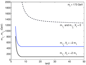
Fig. 2: Minimum physical stop masses, $m_{\tilde{t}_{1}}$ and $m_{\tilde{t}_{2}}$, for $m_{h}\geq 114.4$ GeV as a function of $\tan\beta$ for vanishing stop mixing ($X_{t}=0$) and natural maximal stop mixing ($X_{t}/m_{\tilde{t}}=-2$). Other parameters are as given in Fig. 1.

Within the MSSM, the results from the Higgsstrahlung channel give an upper bound on $\sin^{2}(\beta-\alpha)$ and $\cos^{2}(\beta-\alpha)$ as a function of $m_{h}$ and $m_{H}$, respectively (see Fig. 2 in [1]). The pair production channel, on the other hand, gives an upper bound on $\cos^{2}(\beta-\alpha)$ and $\sin^{2}(\beta-\alpha)$ as a function of $m_{h}+m_{A}$ and $m_{H}+m_{A}$, respectively (see Fig. 4 in [1]). Appendix A contains a review on how these functions of $\alpha$ and $\beta$ appear in the MSSM, and why LEP bounds them.

The LEP results from the Higgsstrahlung channel put several interesting bounds on $m_{h}$, $m_{H}$ and $\sin^{2}(\beta-\alpha)$. In the decoupling limit, $h$ behaves like the SM Higgs so that $\sin^{2}(\beta-\alpha)\rightarrow 1$ and the bound on its mass is given by

$$m_{h}\geq 114.4{\textrm{ GeV}},~{}\sin^{2}(\beta-\alpha)\rightarrow 1.$$ (1)

If $m_{h}$ is less than 114.4 GeV, smaller values of $\sin^{2}(\beta-\alpha)$ are required in order to suppress the production of $h$ in the Higgsstrahlung channel and to allow it to have escaped detection. For $m_{h}$ $\simeq$ 93 GeV, $\sin^{2}(\beta-\alpha)$ needs to be less than about 0.2, so that $\cos^{2}(\beta-\alpha)\gtrsim 0.8$ (from Fig. 2 in [1]). Larger values of $\cos^{2}(\beta-\alpha)$, however, increase the $HZZ$ coupling so that now $m_{H}$ needs to be large enough to suppress the production of $H$ in the Higgsstrahlung channel, and allow it, in turn, to have escaped detection. We find that $m_{H}\gtrsim 114.0$ GeV (from Fig. 2 in [1]). If $\sin^{2}(\beta-\alpha)$ is even smaller and approaches zero, i.e. $\cos^{2}(\beta-\alpha)\rightarrow 1$, it is $H$ which behaves like the SM Higgs so that the bound on its mass is given by $m_{H}$ $\geq$ 114.4 GeV (this will be referred to as the Higgs “non-decoupling” limit).

In Section 3, we present lower bounds on the stop soft masses for two regions in the Higgs parameter space. These two regions are given by equation (1) and by

$$m_{h}\simeq 93{\textrm{ GeV}},~{}\cos^{2}(\beta-\alpha)\geq 0.8,~{}m_{H}\geq 114.4\textrm{ GeV}.$$ (2)

(We choose $m_{H}$ in equation (2) to be at least above 114.4 GeV, in order to allow the full range $0.8\leq\cos^{2}(\beta-\alpha)\leq 1$.)

We note that the bounds given in the previous paragraphs assume that the MSSM Higgs boson $h$ decays like the SM Higgs boson (see [1]). If we assume different Higgs decay branching ratios, somewhat different bounds can be obtained. For example, assuming $h$ decays completely into $\tau\bar{\tau}$ gives a stricter bound on the $hZZ$ coupling for a wide range of $m_{h}$. The LEP collaboration even considered the extreme case in which the Higgs decays invisibly. In this case, the bound on the $hZZ$ coupling as a function of $m_{h}$ is in general not much worse than if we assume that the Higgs decays like a SM Higgs. In fact, for some range of $m_{h}$ the bound is even stricter if we assume that the Higgs decays invisibly [3].

The lower bound on $m_{h}$ is also model dependent. For example, in [1], figures are presented that show excluded regions in the MSSM parameter space for a variety of “benchmark” scenarios that consist of different choices for the MSSM parameters. The LEP collaboration found that the lower bound on $m_{h}$ can be slightly less than 93 GeV in certain cases. Moreover, the authors in [4] claim that there are certain regions in parameter space for which the $ZZh$ coupling and the $h/A\rightarrow b\bar{b}$ branching ratios are both suppressed and that this allows $m_{h}$ to be substantially less than 93 GeV.

2.2 Implications for the MSSM stop sector

Since the tree-level mass of the lighter neutral Higgs is bounded above by $m_{Z}$, it is clear that substantial radiative corrections are required to push the lighter Higgs mass above 114.4 GeV in the Higgs decoupling limit.

We now discuss why substantial radiative corrections to the tree-level Higgs masses are also required if the lighter Higgs mass is near 93 GeV. This is most easily seen in the large $\tan\beta$ limit. In this limit, the CP-even Higgs mass squared matrix in the ($H_{d}$,$H_{u}$) basis is particularly simple if we only include the tree-level pieces and the dominant radiative corrections. Since $\tan\beta$ is large, the vacuum expectation value $v_{d}$ vanishes in this limit, and the Higgs vacuum expectation value is thus completely determined by $v_{u}$. In the absence of any radiative corrections, one of the physical Higgs mass eigenstates lies completely in the $H_{u}$ direction and thus behaves like the SM Higgs (with a mass equal to $m_{Z}$), whereas the other mass eigenstate lies completely in the $H_{d}$ direction (with a mass equal to the mass of the CP-odd Higgs, $m_{A}$). This alignment of the two physical CP-even Higgs mass eigenstates with the $H_{u}$ and $H_{d}$ direction, respectively, remains unchanged when only the dominant radiative correction is added. The reason for this is that, due to the large top Yukawa coupling, the dominant radiative corrections to the Higgs sector are to the up-type Higgs soft supersymmetry breaking Lagrangian mass and come from loops involving the top quark and stop squarks [5, 6, 7]. This gives a correction to the $H_{u}$-$H_{u}$ component of the CP-even Higgs mass squared matrix. The matrix is thus particularly simple for large $\tan\beta$, and is given by

$$\mathcal{M}^{2}\approx\left(\begin{array}[]{cc}m_{A}^{2}&0\\ 0&m_{Z}^{2}+\delta\mathcal{M}^{2}_{uu}\end{array}\right)~{}~{}~{}~{}~{}~{}~{}({\textrm{for large}}~{}\tan\beta),$$ (3)

where $\delta\mathcal{M}^{2}_{uu}$ is the dominant top/stop correction. Since the $H_{u}$-$H_{u}$ component for large $\tan\beta$ gives the mass of the physical Higgs that behaves like the SM Higgs, its value is bounded below by 114.4 GeV, i.e.

$$m_{Z}^{2}+\delta\mathcal{M}^{2}_{uu}\gtrsim(114.4\textrm{ GeV})^{2}.$$ (4)

The result in equation (4) is independent of whether the lighter or the heavier Higgs lies in the $H_{u}$ direction (this depends on the size of $m_{A}$). It also shows that the lower bound on the size of the required radiative corrections is fixed and independent of the mass of the lighter Higgs, at least in the large $\tan\beta$ limit including only the leading corrections. Moreover, it is $m_{H}$ which acquires the dominant radiative corrections for $m_{h}\simeq$ 93 GeV.

A simple estimate of the lower bounds on the stop masses in the large $\tan\beta$ limit may be obtained using equation (4). For large $\tan\beta$, the dominant radiative correction is given by

$$\delta\mathcal{M}^{2}_{uu}\simeq\frac{3g^{2}m_{t}^{4}}{8\pi^{2}m_{W}^{2}}\Bigg{\{}\ln\Bigg{(}\frac{m_{\tilde{t}}^{2}}{m_{t}^{2}}\Bigg{)}+\frac{X_{t}^{2}}{m_{\tilde{t}}^{2}}\Bigg{(}1-\frac{X_{t}^{2}}{12m_{\tilde{t}}^{2}}\Bigg{)}\Bigg{\}},$$ (5)

where $m_{t}$ is the top mass, $g$ is the $SU(2)_{L}$ gauge coupling, and $m_{W}$ is the mass of the $W$-bosons [5, 6, 7]. Furthermore, equation (5) assumes that the stop soft masses are equal to $m_{\tilde{t}}$, with $m_{\tilde{t}}$ $\gg$ $m_{t}$. The stop mixing parameter is given by $X_{t}=A_{t}-\mu\cot\beta$ ($\simeq$ $A_{t}$ for large $\tan\beta$), where $A_{t}$ denotes the stop soft trilinear coupling and $\mu$ is the supersymmetric Higgsino mass parameter. The dependence on the top mass to the fourth power is particularly noteworthy. The first term in equation (5) comes from renormalization group running of the Higgs quartic coupling below the stop mass scale and vanishes in the limit of exact supersymmetry. It grows logarithmically with the stop mass. The second term is only present for non-zero stop mixing and comes from a finite threshold correction to the Higgs quartic coupling at the stop mass scale. It is independent of the stop mass for fixed $X_{t}/m_{\tilde{t}}$, and grows linearly as $(X_{t}/m_{\tilde{t}})^{2}$ for small $X_{t}/m_{\tilde{t}}$.

It is apparent from equation (5) that the mixing term is important for determining lower bounds on the stop masses. Using equation (5) and assuming no mixing ($X_{t}=0$), we require $m_{\tilde{t}}\gtrsim 570$ GeV in order to satisfy the LEP bound in (4). This value was obtained using a running top mass of $m_{t}(m_{t})\simeq 167$ GeV [8]. The second (mixing) term in equation (5), however, reaches a maximum of 3 for $X_{t}=\sqrt{6}m_{\tilde{t}}$, called maximal-mixing. In order for the logarithm of the first term to be of the same order, $m_{\tilde{t}}$ needs to be about 750 GeV. Thus the mixing term alone is more than enough to give the required radiative corrections to satisfy the LEP bound. Mixing in the stop sector therefore allows for much smaller stop masses.

There are other radiative corrections to the Higgs masses which are important, including negative radiative corrections that come from charginos, for example. In Section 3, we include all the important radiative corrections to determine more accurate lower bounds on the stop masses. For example, for no stop mixing and $\tan\beta=50$, a more accurate lower bound is given by $m_{\tilde{t}}\gtrsim$ 980 GeV, assuming a physical top mass of 173 GeV, $\mu=200$ GeV, and a bino and wino mass of 100 GeV and 200 GeV, respectively. This shows the importance of including higher order corrections to the Higgs sector. Moreover, the lower bound is approximately the same for $m_{h}\simeq 93$ GeV and for $m_{h}\geq 114.4$ GeV, as expected for large $\tan\beta$.

The above discussion assumes that $\tan\beta$ is large. In Section 3, we obtain lower bounds on $m_{\tilde{t}}$ also for small and moderate values of $\tan\beta$, for which the off-diagonal elements in the Higgs mass matrix become important. In general, we find that the stop masses and/or mixing have to be sizeable for all values of $\tan\beta$ and for both the Higgs decoupling and non-decoupling regions. However, depending on the size of the stop mixing, the lower bounds on the stop masses for moderate values of $\tan\beta$ can be smaller for $m_{h}\simeq 93$ GeV than for $m_{h}\geq 114.4$ GeV (see also [9]). Moreover, for small values of $\tan\beta$, the lower bounds on the stop masses become larger for $m_{h}\simeq 93$ GeV than for $m_{h}\geq 114.4$ GeV.

3 Lower bounds on the stop masses

In this section, we present lower bounds on the stop masses consistent with the LEP Higgs bounds, and we discuss their dependence on some of the other MSSM parameters. In particular, we set lower bounds on the left-handed and right-handed stop soft mass, $m_{\tilde{t}_{L}}$ and $m_{\tilde{t}_{R}}$, respectively, taking both equal to a common value, which we denote by $m_{\tilde{t}}$. We denote the lower bound on $m_{\tilde{t}}$ consistent with the LEP Higgs bounds by $m_{\tilde{t},\textrm{\tiny{min}}}$. We consider the two scenarios given in equations (1) and (2), namely the Higgs decoupling limit with $m_{h}\geq 114.4$ GeV (Section 3.1), and near the Higgs non-decoupling limit with $m_{h}\simeq 93$ GeV, and the additional constraints $\cos^{2}(\beta-\alpha)\geq 0.8$ and $m_{H}\geq 114.4$ GeV (Section 3.3). In addition, in Section 3.2, we give lower bounds on the stop soft masses as a function of the physical Higgs boson mass $m_{h}$ in the decoupling limit. All the lower bounds on the stop masses that we present are consistent with the 2$\sigma$ constraint on $\delta\rho$ (which is related to the electroweak $T$-parameter). In Section 4, we discuss the importance of this parameter, as well as others, in constraining the stop masses.

3.1 Lower bounds on the stop masses for $m_{h}\geq 114.4$ GeV

For a given set of parameters, we minimize $m_{\tilde{t}}$ by starting it at the lowest value that gives physical stop masses above 100 GeV and increasing it until $m_{h}$ is above 114.4 GeV. We choose the physical stop mass to be at least 100 GeV since this bound is illustrative of the actual, slightly model dependent, lower bound obtained from the Tevatron [10]. The Higgs masses were calculated with version 2.2.7 of the program $\mathtt{FeynHiggs}$ which includes all the important radiative corrections to the Higgs sector [11, 12, 13, 14]. We set $m_{A}=1000$ GeV to ensure that we are in the Higgs decoupling limit.

In Fig. 1, we show $m_{\tilde{t},\textrm{\tiny{min}}}$ as a function of $\tan\beta$ for stop mixing $X_{t}/m_{\tilde{t}}$ $=$ $0$, $\pm 1$, and $\pm 2$. All squark, slepton, and gaugino soft masses are equal to $m_{\tilde{t}}$, $\mu=200$ GeV, $m_{t}=173$ GeV, and all the soft trilinear couplings are equal to the stop soft trilinear coupling, $A_{t}=X_{t}+\mu\cot\beta$. The lower solid line shows the maximal-mixing scenario, $X_{t}=2m_{\tilde{t}}$, which approximately maximizes the radiative corrections to the Higgs sector for a given set of parameters [17]. The dot-dashed line shows the no-mixing scenario, $X_{t}=0$, which approximately minimizes the radiative corrections to the Higgs sector for a given set of parameters. The lower dashed line shows the results for $X_{t}=m_{\tilde{t}}$. An intermediate-mixing scenario with $X_{t}=-m_{\tilde{t}}$ is represented by the upper dashed line. We choose this scenario since $A_{t}$ has a strongly attractive infrared quasi-fixed point at $A_{t}$ = $-M_{3}$, see Appendix B. Thus, $A_{t}$ prefers to be negative due to renormalization group evolution from the high scale down to the low scale (we choose the convention in which $M_{3}$ is positive). In addition, we consider a scenario which maximizes the Higgs mass for negative stop mixing, and call it natural maximal mixing. This scenario is given by $X_{t}=-2m_{\tilde{t}}$ and is represented by the upper solid-line in the figure.

A feature that is common to all the curves is that $m_{\tilde{t}}$ becomes very large for small $\tan\beta$. This is because the tree-level contribution to the Higgs mass in the decoupling limit is given by $m_{h}^{\textrm{\tiny{tree}}}$ $\simeq$ $|\!\cos 2\beta|m_{Z}$, and goes to zero as $\tan\beta$ approaches 1. Larger radiative corrections, and thus larger stop masses, are therefore required for smaller $\tan\beta$ to push $m_{h}$ above 114.4 GeV.

Fig. 1 clearly shows that mixing in the stop sector has a large impact on the values of $m_{\tilde{t},\textrm{\tiny{min}}}$, with larger mixing allowing much smaller values of $m_{\tilde{t},\textrm{\tiny{min}}}$ (see also [18, 19]). For large $\tan\beta$, the difference in $m_{\tilde{t},\textrm{\tiny{min}}}$ between no mixing and maximal mixing is about 1000 GeV, with $m_{\tilde{t},\textrm{\tiny{min}}}=1260$ GeV for $\tan\beta=50$ in the no-mixing case.

A plot of the two physical stop masses, $m_{\tilde{t}_{1}}$ and $m_{\tilde{t}_{2}}$, versus $\tan\beta$ is given in Fig. 2 for no mixing and for natural maximal mixing. For no mixing, there is no discernible difference in the two stop masses since the only difference that arises is from small $SU(2)_{L}$ and $U(1)_{Y}$ D-term quartic interactions. For appreciable mixing, the two physical stop masses are split by an amount that is on the order of $\sim\sqrt{m_{t}X_{t}}$. For $X_{t}=-2m_{\tilde{t}}$ and $\tan\beta\geq 7$, $m_{\tilde{t},\textrm{\tiny{min}}}$ is small enough that the lighter physical stop mass is all the way down at its experimental lower bound of roughly 100 GeV. For this range of $\tan\beta$, we find that $m_{\tilde{t}}$ is larger than that which is required to get $m_{h}$ just above 114.4 GeV, and thus $m_{h}$ is several GeV above 114.4 GeV here.

The current value of the top mass from the CDF and D0 experiments at Fermilab is $m_{t}=171.4\pm 2.1$ GeV [20]. The values obtained for $m_{\tilde{t},\textrm{\tiny{min}}}$ are, however, extremely sensitive to slight variations in the value of the top mass (see also [18]). It is thus illustrative to plot $m_{\tilde{t},\textrm{\tiny{min}}}$ as a function of $\tan\beta$ for various amounts of stop mixing and for three choices of the top mass: 168 GeV, 173 GeV and 178 GeV. The plots are shown in Fig. 3, 4 and 5 for $X_{t}/m_{\tilde{t}}$ = 0, -1, and -2, respectively. These plots again assume that all squark, slepton, and gaugino soft masses are equal to $m_{\tilde{t}}$, $\mu=200$ GeV, and all the soft trilinear couplings are equal to $A_{t}$.

All three figures show that $m_{\tilde{t},\textrm{\tiny{min}}}$ is extremely sensitive to small changes in $m_{t}$ for small $\tan\beta$. For intermediate and vanishing stop mixing, this sensitivity persists for large $\tan\beta$. For example, in the no-mixing case for $\tan\beta=50$, we find $m_{\tilde{t},\textrm{\tiny{min}}}\simeq$ 870 GeV, 1260 GeV, and 2570 GeV for $m_{t}=$ 178 GeV, 173 GeV, and 168 GeV, respectively. The very large value of $m_{\tilde{t},\textrm{\tiny{min}}}$ for $m_{t}=168$ GeV is particularly noteworthy, especially if the central value of the measured top mass keeps decreasing slightly as more data from the Tevatron becomes available.

So far we assumed that the gaugino masses are all equal to $m_{\tilde{t}}$. The bino and wino masses, $M_{1}$ and $M_{2}$, as well as $\mu$ contribute to the Higgs masses at one loop, whereas the gluino mass, $M_{3}$, only appears at two loops (see e.g. [8, 12, 21] and references therein). Since large values of $M_{1}$, $M_{2}$ and $\mu$ can give important negative contributions to the Higgs masses [22], smaller values of $m_{\tilde{t},\textrm{\tiny{min}}}$ are possible for smaller values of $M_{1}$, $M_{2}$ and $\mu$. For example, setting $M_{1}$ = 100 GeV, $M_{2}$ = 200 GeV and $M_{3}$ = 800 GeV, we find in the no-mixing case for $\tan\beta=50$ that $m_{\tilde{t},\textrm{\tiny{min}}}\simeq$ 760 GeV, 980 GeV, and 1410 GeV for $m_{t}=$ 178 GeV, 173 GeV and 168 GeV, respectively. This may be compared with the values given in the previous paragraph for the case where all the gaugino masses are equal to $m_{\tilde{t}}$. Thus, setting the bino and wino masses to smaller values decreases the size of $m_{\tilde{t},\textrm{\tiny{min}}}$, especially if $m_{t}$ is small. However, the large value of $m_{\tilde{t},\textrm{\tiny{min}}}$ for $m_{t}=168$ GeV is still noteworthy.

We show a further example of how a different choice for $M_{1}$ and $M_{2}$ affects $m_{\tilde{t},\textrm{\tiny{min}}}$ in Fig. 6 for the no-mixing and natural-maximal-mixing scenario. For each scenario, this figure shows a case for which $M_{1}$ and $M_{2}$ are both large ($M_{1}=M_{2}=$ 800 GeV) or both small ($M_{1}$ = 100 GeV, $M_{2}$ = 200 GeV). In both cases, $M_{3}$ is fixed to be 800 GeV, $\mu=200$ GeV, $m_{t}=173$ GeV, all squark and slepton soft masses are equal to the stop soft masses, and all the soft trilinear couplings are equal to $A_{t}$. The plots show that $m_{\tilde{t},\textrm{\tiny{min}}}$ is smaller for smaller values of $M_{1}$ and $M_{2}$. For example, $m_{\tilde{t},\textrm{\tiny{min}}}$ is about 160 GeV smaller in the no-mixing case for $\tan\beta=50$ when choosing the smaller set of values for $M_{1}$ and $M_{2}$, and the difference in $m_{\tilde{t},\textrm{\tiny{min}}}$ grows as $\tan\beta$ decreases. For natural maximal mixing, no difference can be seen for most $\tan\beta$ values, since here the condition $m_{\tilde{t}_{1}}\geq 100$ GeV again requires larger values of $m_{\tilde{t},\textrm{\tiny{min}}}$ than the condition $m_{h}\geq 114.4$ GeV. However, there is a difference in $m_{\tilde{t},\textrm{\tiny{min}}}$ for smaller $\tan\beta$, which again grows as $\tan\beta$ decreases.

Fig. 6 also shows how a change in the gluino mass, $M_{3}$, affects $m_{\tilde{t},\textrm{\tiny{min}}}$. In general, $m_{h}$ tends to be maximized for $M_{3}$ $\simeq$ $0.8m_{\tilde{t}}$ [12]. In this figure, we compare $m_{\tilde{t},\textrm{\tiny{min}}}$ for two different gluino masses, namely $M_{3}=800$ GeV and $M_{3}=1500$ GeV. The figure shows that the effect is not very large for this choice of parameters. However, the gluino mass can significantly affect the Higgs masses, and therefore $m_{\tilde{t},\textrm{\tiny{min}}}$, for large $\tan\beta$ and large and negative $\mu$.

The variation of $m_{h}$ as a function of $\mu$ does not generally exceed about 3 GeV [12]. However, it can become very large if one includes the all-order resummation of the $\tan\beta$ enhanced terms of order $\mathcal{O}(\alpha_{b}(\alpha_{s}\tan\beta)^{n})$, where $\alpha_{b}=\lambda_{b}^{2}/4\pi$ and $\lambda_{b}$ is the bottom Yukawa coupling [23, 24, 25, 26, 27, 28, 29]. This resummation is included in $\mathtt{FeynHiggs}$. The origin of the enhancement is a change in the bottom Yukawa coupling due to a loop containing, for example, a gluino and a sbottom squark. The leading corrections to the bottom Yukawa coupling can be incorporated into the one-loop result for the Higgs masses by the use of an effective bottom mass, $m_{b}^{\textrm{\tiny{eff}}}$. Large $|\mu|\tan\beta$ can substantially change the effective bottom mass $m_{b}^{\textrm{\tiny{eff}}}$ from its $\overline{\textrm{MS}}$ value. Positive $\mu$ can substantially decrease $m_{b}^{\textrm{\tiny{eff}}}$, making the sbottom/bottom sector corrections to $m_{h}$ negligible. Negative $\mu$ on the other hand can substantially increase $m_{b}^{\textrm{\tiny{eff}}}$, making the sbottom/bottom sector corrections to $m_{h}$ important. The bottom/sbottom corrections to $m_{h}$ are negative in the latter case. Larger stop masses are then required for large and negative $\mu$ as $\tan\beta$ increases to enhance the positive radiative corrections from the stop/top.

This effect can be seen in Fig. 7 where we compare $\mu=+200$ GeV and $\mu=\pm 500$ GeV for natural maximal stop mixing. This figure again assumes that all squark, slepton, and gaugino soft masses are equal to the stop soft masses, $m_{t}=173$ GeV, and all the soft trilinear couplings are equal to $A_{t}$. For large $\tan\beta$, slightly larger $m_{\tilde{t},\textrm{\tiny{min}}}$ are required for $\mu=-500$ GeV than when $\mu$ is positive (the effect would be stronger for even larger negative $\mu$). Note that for small values of $\tan\beta$ there is a region for which $m_{\tilde{t}}$ is larger for both $\mu=-500$ GeV and $\mu=+500$ GeV than for $\mu=200$ GeV. As we discussed above, this is because larger chargino and neutralino masses decrease the size of $m_{h}$.

Since the gluino mass also enters the equation that determines $m_{b}^{\textrm{\tiny{eff}}}$, it can have a significant impact on $m_{h}$ for large $\tan\beta$ and large negative values of $\mu$ as demonstrated in [29]. Thus, some non-negligible dependence of $m_{\tilde{t},\textrm{\tiny{min}}}$ on the gluino mass is expected for negative and large $\mu$.

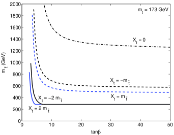
Fig. 1: Minimum stop soft masses, $m_{\tilde{t}}\equiv m_{\tilde{t}_{L}}=m_{\tilde{t}_{R}}$, for $m_{h}\geq 114.4$ GeV as a function of $\tan\beta$ for stop mixing $X_{t}/m_{\tilde{t}}=0,\pm 1,\pm 2$. All squark, slepton, and gaugino soft masses are equal to the stop soft masses, $\mu=200$ GeV, $m_{A}=1000$ GeV, $m_{t}=173$ GeV, and all soft trilinear couplings are equal to $A_{t}=X_{t}+\mu\cot\beta$.

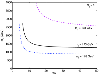
Fig. 3: Minimum stop soft masses, $m_{\tilde{t}}\equiv m_{\tilde{t}_{L}}=m_{\tilde{t}_{R}}$, for $m_{h}\geq 114.4$ GeV as a function of $\tan\beta$ for vanishing stop mixing ($X_{t}=0$) for a top quark mass of $m_{t}=168,173,178$ GeV. Other parameters are as given in Fig. 1.

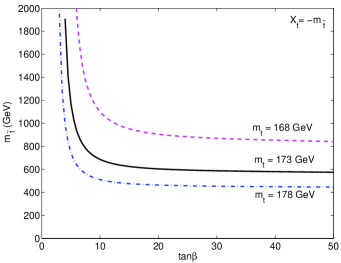
Fig. 4: Minimum stop soft masses, $m_{\tilde{t}}\equiv m_{\tilde{t}_{L}}=m_{\tilde{t}_{R}}$, for $m_{h}\geq 114.4$ GeV as a function of $\tan\beta$ for intermediate stop mixing ($X_{t}/m_{\tilde{t}}=-1$) for a top quark mass of $m_{t}=168,173,178$ GeV. Other parameters are as given in Fig. 1.

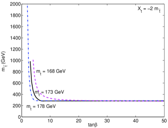
Fig. 5: Minimum stop soft masses, $m_{\tilde{t}}\equiv m_{\tilde{t}_{L}}=m_{\tilde{t}_{R}}$, for $m_{h}\geq 114.4$ GeV as a function of $\tan\beta$ for natural maximal stop mixing ($X_{t}/m_{\tilde{t}}=-2$) for a top quark mass of $m_{t}=168,173,178$ GeV. Other parameters are as given in Fig. 1.

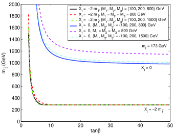
Fig. 6: Minimum stop soft masses, $m_{\tilde{t}}\equiv m_{\tilde{t}_{L}}=m_{\tilde{t}_{R}}$, for $m_{h}\geq 114.4$ GeV as a function of $\tan\beta$ for various values of the bino, wino, and gluino soft masses, $M_{1},M_{2},M_{3}$. The upper three lines are for vanishing stop mixing ($X_{t}=0$) and the lower three for natural maximal stop mixing ($X_{t}/m_{\tilde{t}}=-2$). Other parameters are as given in Fig. 1.

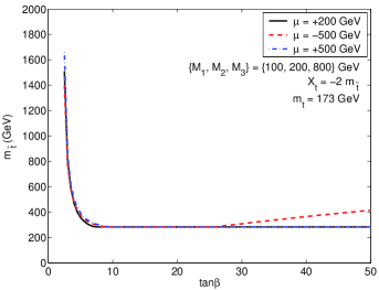
Fig. 7: Minimum stop soft masses, $m_{\tilde{t}}\equiv m_{\tilde{t}_{L}}=m_{\tilde{t}_{R}}$, for $m_{h}\geq 114.4$ GeV as a function of $\tan\beta$ for natural maximal stop mixing ($X_{t}/m_{\tilde{t}}=-2$) with $\mu=-500,200,500$ GeV and bino, wino, and gluino soft masses of $M_{1}=100$ GeV, $M_{2}=200$ GeV, $M_{3}=800$ GeV. Other parameters are as given in Fig. 1.

3.2 Lower bounds on the stop masses as function of the Higgs mass

In this section, we present lower bounds on the stop soft masses, $m_{\tilde{t}}\equiv m_{\tilde{t}_{L}}=m_{\tilde{t}_{R}}$, as a function of the Higgs mass, $m_{h}$. We assume the decoupling limit ($m_{A}=1000$ GeV), and we set all squark and slepton soft masses equal to the stop soft masses, $\mu=200$ GeV, $m_{t}=173$ GeV, $M_{1}$ = 100 GeV, $M_{2}$ = 200 GeV, $M_{3}$ = 800 GeV, $\tan\beta=30$, and all the soft trilinear couplings equal to $A_{t}$. We allow $m_{h}$ to range from 100 GeV upwards. This means that the values obtained for $m_{\tilde{t}}$ in the range $m_{h}\in[100,114.4]$ GeV will be lower than those consistent with the LEP results, since we set no additional constraints on $\cos^{2}(\beta-\alpha)$ and $m_{H}$. However, the main point here is to show the dependence of $m_{\tilde{t}}$ on $m_{h}$ without any other constraints. The lower bounds on $m_{\tilde{t}}$ are required to give physical stop masses not less than 100 GeV.

We show the results for different amounts of stop mixing in Fig. 8. This figure shows how an increase in $m_{h}$ requires an exponential increase in $m_{\tilde{t}}$. In addition to the no-mixing, intermediate-mixing and natural-maximal-mixing cases, we also include the $m_{h}^{\textrm{\tiny{max}}}$ benchmark scenario ($X_{t}=+2m_{\tilde{t}}$) (but with $\mu=+200$ GeV, not $\mu=-200$ GeV) [22]. This benchmark scenario is designed to maximize the Higgs mass for a given set of parameters. Moreover, we choose $M_{3}=800$ GeV for all cases, with the exception of the latter one. In the latter benchmark scenario, we choose the benchmark value $M_{3}=0.8m_{\tilde{t}}$ instead, which gives slightly higher values for $m_{h}$ [22].

It is clear from the figure that there is some value of $m_{h}$ at which a further small increase in $m_{h}$ would require an extremely large increase in the stop masses. It is instructive to obtain the values of $m_{h}$ from the figure if, for example, $m_{\tilde{t}}$ = 3000 GeV. We find for no stop mixing, $m_{h}\simeq 121$ GeV, for intermediate stop mixing, $m_{h}\simeq 126$ GeV, for natural maximal stop mixing, $m_{h}\simeq 131$ GeV, and for the $m_{h}^{\textrm{\tiny{max}}}$ benchmark scenario, $m_{h}\simeq 134$ GeV (see also [30], for example, and references therein).

Since $A_{t}$ and $M_{3}$ most naturally have the opposite sign due to renormalization group running and the presence of a strongly attractive quasi-fixed point (see Appendix B), a negative value of $A_{t}$ is more natural. For negative $A_{t}$, the upper bound of $m_{h}$ in the MSSM is around 131 GeV.

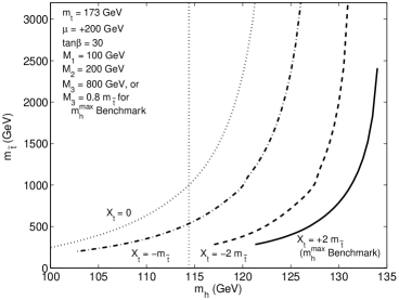
Fig. 8: Minimum stop soft masses, $m_{\tilde{t}}\equiv m_{\tilde{t}_{L}}=m_{\tilde{t}_{R}}$, as a function of $m_{h}$. All squark and slepton soft masses are equal to the stop soft masses, $\mu=200$ GeV, $m_{t}=173$ GeV, $\{M_{1},M_{2}\}$ = $\{100,200\}$ GeV, $\tan\beta=30$, and all the soft trilinear couplings are equal to $A_{t}=X_{t}+\mu\cot\beta$. In the figure, the curved lines from left to right are as follows: the dotted line is for no mixing ($X_{t}/m_{\tilde{t}}=0$), the dash-dot line for intermediate mixing ($X_{t}/m_{\tilde{t}}=-1$), the dashed line for natural maximal mixing ($X_{t}/m_{\tilde{t}}=-2$), and the solid line for the $m_{h}^{\textrm{\tiny{max}}}$ benchmark scenario ($X_{t}/m_{\tilde{t}}=+2$) [22]. The gluino mass is set to be $M_{3}$ = 800 GeV in all cases except in the $m_{h}^{\textrm{\tiny{max}}}$ benchmark scenario, where $M_{3}=0.8m_{\tilde{t}}$. The vertical dotted line is at $m_{h}=114.4$ GeV, which is the lower bound set by LEP on $m_{h}$ in the decoupling limit.

3.3 Lower bounds on the stop masses for $m_{h}\simeq 93$ GeV

In this section, we present results for the minimum stop soft masses, $m_{\tilde{t}}\equiv m_{\tilde{t}_{L}}=m_{\tilde{t}_{R}}$, as a function of $\tan\beta$, for various choices of the other MSSM parameters, and consistent with the following set of constraints on the Higgs sector obtained by LEP: $m_{h}\simeq 93$ GeV, $\cos^{2}(\beta-\alpha)\geq 0.8$ and $m_{H}\geq 114.4$ GeV (see equation (2)).

The mass $m_{A}$ is allowed to be a free parameter, since $m_{\tilde{t}}$ needs to be minimized without enforcing the decoupling limit. We vary $m_{A}$ between 93.5 GeV and 1000 GeV from the bottom up for a given choice of $m_{\tilde{t}}$ and other MSSM parameters, until the conditions 93 GeV $\leq$ $m_{h}$ $\leq$ 95 GeV, $\cos^{2}(\beta-\alpha)\geq 0.8$, and $m_{H}\geq 114.4$ GeV are satisfied. (The lower bound of 93.5 GeV for $m_{A}$ is the approximate lower bound obtained within the same benchmark scenarios as the bound on $m_{h}$; it turns out that the actual values obtained for $m_{A}$ are slightly larger). If these conditions cannot all be satisfied, we keep increasing $m_{\tilde{t}}$ until they are satisfied. Note that we require the lower bounds on $m_{\tilde{t}}$ to give physical stop masses of at least 100 GeV. We again denote the lower bounds on $m_{\tilde{t}}$ consistent with the LEP Higgs bounds by $m_{\tilde{t},\textrm{\tiny{min}}}$.

The Higgs masses, $m_{h}$ and $m_{H}$, are calculated with $\mathtt{FeynHiggs}$, and $\cos^{2}(\beta-\alpha)$ is calculated using the $\mathtt{FeynHiggs}$ output of the radiatively corrected CP-even Higgs mixing angle $\alpha$.

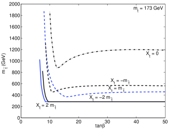
Fig. 9: Minimum stop soft masses, $m_{\tilde{t}}\equiv m_{\tilde{t}_{L}}=m_{\tilde{t}_{R}}$, for $m_{h}\simeq 93$ GeV, $m_{H}\geq 114.4$ GeV, and $\cos^{2}(\beta-\alpha)\geq 0.8$, as a function of $\tan\beta$ for stop mixing $X_{t}/m_{\tilde{t}}=0,\pm 1,\pm 2$. All squark, slepton, and gaugino soft mass parameters are equal to the stop soft masses, $\mu=200$ GeV, $m_{t}=173$ GeV, and all soft trilinear couplings are equal to $A_{t}=X_{t}+\mu\cot\beta$. This figure may be compared with Fig. 1.

In Fig. 9, we show $m_{\tilde{t},\textrm{\tiny{min}}}$ as a function of $\tan\beta$ for stop mixing $X_{t}/m_{\tilde{t}}$ $=$ $0$, $\pm 1$, and $\pm 2$. All squark, slepton, and gaugino soft masses are equal to the stop soft masses, $\mu=200$ GeV, $m_{t}=173$ GeV, and all the soft trilinear couplings are equal to the stop soft trilinear coupling, $A_{t}$. This figure may be compared with Fig. 1 in which we require $m_{h}\geq 114.4$ GeV in the Higgs decoupling limit.

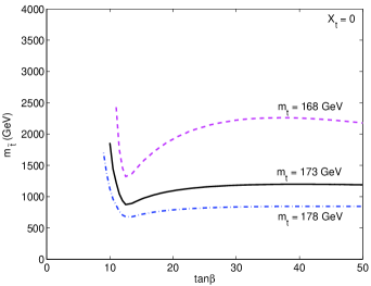
Fig. 10: Minimum stop soft masses, $m_{\tilde{t}}\equiv m_{\tilde{t}_{L}}=m_{\tilde{t}_{R}}$, for $m_{h}\simeq 93$ GeV, $m_{H}\geq 114.4$ GeV, and $\cos^{2}(\beta-\alpha)\geq 0.8$, as a function of $\tan\beta$ for vanishing stop mixing ($X_{t}/m_{\tilde{t}}=0$) for a top quark mass of $m_{t}=168,173,178$ GeV. Other parameters are given as in Fig. 9. This figure may be compared with Fig. 3.

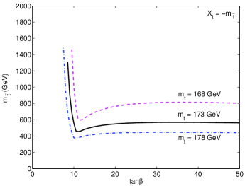
Fig. 11: Minimum stop soft masses, $m_{\tilde{t}}\equiv m_{\tilde{t}_{L}}=m_{\tilde{t}_{R}}$, for $m_{h}\simeq 93$ GeV, $m_{H}\geq 114.4$ GeV, and $\cos^{2}(\beta-\alpha)\geq 0.8$, as a function of $\tan\beta$ for intermediate stop mixing ($X_{t}/m_{\tilde{t}}=-1$) for a top quark mass of $m_{t}=168,173,178$ GeV. Other parameters are given as in Fig. 9. This figure may be compared with Fig. 4.

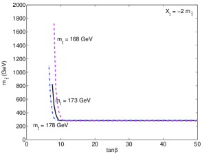
Fig. 12: Minimum stop soft masses, $m_{\tilde{t}}\equiv m_{\tilde{t}_{L}}=m_{\tilde{t}_{R}}$, for $m_{h}\simeq 93$ GeV, $m_{H}\geq 114.4$ GeV, and $\cos^{2}(\beta-\alpha)\geq 0.8$, as a function of $\tan\beta$ for natural maximal stop mixing ($X_{t}/m_{\tilde{t}}=-2$) for a top quark mass of $m_{t}=168,173,178$ GeV. Other parameters are given as in Fig. 9. This figure may be compared with Fig. 5.

Next, we show $m_{\tilde{t},\textrm{\tiny{min}}}$ as a function of $\tan\beta$ for different values of the top mass (168 GeV, 173 GeV and 178 GeV) and for different amounts of mixing. Fig. 10 is for no mixing, Fig. 11 is for intermediate mixing, and Fig. 12 is for natural maximal mixing. All squark, slepton, and gaugino soft masses are again equal to the stop soft masses, $\mu=200$ GeV, and all the soft tri-linear couplings are equal to $A_{t}$. These figures may be compared with the figures in which we require $m_{h}\geq 114.4$ GeV in the decoupling limit, namely Figs. 3, 4 and 5, respectively.

We first compare $m_{\tilde{t},\textrm{\tiny{min}}}$ in the two scenarios $m_{h}\simeq 93$ GeV and $m_{h}\geq 114.4$ GeV for large $\tan\beta$. Here, the figures show that $m_{\tilde{t},\textrm{\tiny{min}}}$ is the same in the case of maximal or natural maximal mixing. For intermediate and vanishing stop mixing, $m_{\tilde{t},\textrm{\tiny{min}}}$ is only slightly smaller for $m_{h}\simeq 93$ GeV than for $m_{h}\geq 114.4$ GeV. Assuming $m_{t}$ = 173 GeV and $\tan\beta=50$, the difference is only about 15 GeV for $X_{t}$ = $-m_{\tilde{t}}$ and 70 GeV for $X_{t}$ = 0. We expected the values for $m_{\tilde{t},\textrm{\tiny{min}}}$ to be so similar from the discussion in Section 2.2.

For moderate $\tan\beta$, $m_{\tilde{t},\textrm{\tiny{min}}}$ can be substantially smaller for $m_{h}\simeq 93$ GeV than for $m_{h}\geq 114.4$ GeV. This is true in particular for the no-mixing and intermediate-mixing cases, with the difference being more pronounced for smaller values of $m_{t}$. For example, the maximum difference between $m_{\tilde{t},\textrm{\tiny{min}}}$ in the two scenarios is about 600 GeV for $\tan\beta=12.5$ if there is no mixing and $m_{t}=173$ GeV.

As $\tan\beta$ decreases further, however, $m_{\tilde{t},\textrm{\tiny{min}}}$ for $m_{h}\simeq 93$ GeV rises very steeply, and becomes larger than for $m_{h}\geq 114.4$ GeV.

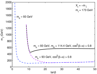
Fig. 14: Minimum stop soft masses, $m_{\tilde{t}}\equiv m_{\tilde{t}_{L}}=m_{\tilde{t}_{R}}$, as a function of $\tan\beta$, for intermediate stop mixing ($X_{t}/m_{\tilde{t}}=-1$). The other parameters and the different lines are as for Fig. 13.

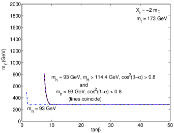
Fig. 15: Minimum stop soft masses, $m_{\tilde{t}}\equiv m_{\tilde{t}_{L}}=m_{\tilde{t}_{R}}$, as a function of $\tan\beta$, for natural maximal stop mixing ($X_{t}/m_{\tilde{t}}=-2$). The other parameters and the different lines are as for Fig. 13.

Understanding this behavior of $m_{\tilde{t},\textrm{\tiny{min}}}$ as a function of $\tan\beta$ requires an understanding of the importance of the constraints $\cos^{2}(\beta-\alpha)\geq 0.8$ and $m_{H}\geq 114.4$ GeV. To this end, we compare $m_{\tilde{t},\textrm{\tiny{min}}}$ versus $\tan\beta$ for the case that the constraint on $m_{H}$ is ignored, for the case that both constraints are ignored, and for the case consistent with the LEP bounds that includes both constraints. We again make the comparison for various amounts of mixing in the stop sector. Fig. 13 shows the results for no mixing, Fig. 14 for intermediate mixing, and Fig. 15 for natural maximal mixing. Each of these figures has three lines. The solid line shows the results which are consistent with the LEP bounds, i.e. it includes the two constraints $\cos^{2}(\beta-\alpha)\geq 0.8$ and $m_{H}\geq 114.4$ GeV, in addition to requiring $m_{h}\simeq 93$ GeV. The dashed line, on the other hand, does not include the constraint on $m_{H}$, but does require $\cos^{2}(\beta-\alpha)\geq 0.8$ and $m_{h}\simeq 93$ GeV. The dash-dot line only requires $m_{h}\simeq 93$ GeV, and ignores the constraints on $\cos^{2}(\beta-\alpha)$ and $m_{H}$.

As expected, both constraints from LEP in general increase $m_{\tilde{t},\textrm{\tiny{min}}}$. The constraint $\cos^{2}(\beta-\alpha)\geq 0.8$ is more important as $\tan\beta$ becomes smaller, but less important as $\tan\beta$ gets larger. The constraint $m_{H}\geq 114.4$ GeV, however, is more important for larger $\tan\beta$ (if stop mixing is not too large), but is less important as $\tan\beta$ becomes smaller. We now explain these observations.

If the only condition is $m_{h}\simeq 93$ GeV, the theory tends to be in the Higgs decoupling limit where $\cos^{2}(\beta-\alpha)$ $\rightarrow$ 0. The reason for this is that for a given set of parameters, including a given value of $m_{\tilde{t}}$, $m_{h}$ is maximized in the decoupling limit. (This is also the reason why ignoring both constraints is in general equivalent to ignoring only the constraint $\cos^{2}(\beta-\alpha)$ $\geq$ 0.8 but keeping $m_{H}\geq 114.4$ GeV as a constraint.) The constraint $\cos^{2}(\beta-\alpha)\geq 0.8$, however, forces all the MSSM Higgs masses to be quite small. In particular, $m_{A}$ is forced to be relatively small and degenerate with $m_{h}$, so that larger $m_{\tilde{t}}$ are required to obtain the same value for $m_{h}$. Moreover, the maximum value reached by $\cos^{2}(\beta-\alpha)$ decreases as $\tan\beta$ decreases. Larger radiative corrections, in particular larger values of $m_{\tilde{t}}$ or more stop mixing, can increase the maximum value of $\cos^{2}(\beta-\alpha)$. However, if $\tan\beta$ decreases too far, exponentially larger values of $m_{\tilde{t}}$ are required to allow $\cos^{2}(\beta-\alpha)$ to be greater than 0.8.

For a given set of parameters, $m_{h}$ in general decreases as $\tan\beta$ decreases. This is not the case for $m_{H}$, which in general decreases as $\tan\beta$ increases. This explains why the constraint on $m_{H}$ is more important for larger values of $\tan\beta$. In the decoupling limit, $m_{H}$ is approximately degenerate with $m_{A}$, and larger values of $m_{\tilde{t}}$ do not affect $m_{H}$ much. In the non-decoupling limit, however, larger values of $m_{\tilde{t}}$ can increase $m_{H}$. In fact, if we define $m_{h}^{\textrm{\tiny{max}}}$ to be equal to $m_{h}$ in the decoupling limit, then $m_{H}$ $\simeq$ $m_{h}^{\textrm{\tiny{max}}}$ for large $\tan\beta$ and $\cos^{2}(\beta-\alpha)\simeq 1$. This may be explained with the formula

$$m_{h}^{2}\sin^{2}(\beta-\alpha)+m_{H}^{2}\cos^{2}(\beta-\alpha)=(m_{h}^{\textrm{\tiny{max}}})^{2},$$ (6)

valid for large $\tan\beta$ [30, 31, 32], and explains why larger $m_{\tilde{t}}$ increases the value of $m_{H}$ in, or near, the non-decoupling region (see also Section 2.2).

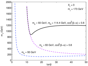
Fig. 13: Minimum stop soft masses, $m_{\tilde{t}}\equiv m_{\tilde{t}_{L}}=m_{\tilde{t}_{R}}$, as a function of $\tan\beta$, for no stop mixing ($X_{t}/m_{\tilde{t}}=0$). The solid line shows the minimum stop soft masses for $m_{h}\simeq 93$ GeV, $m_{H}\geq 114.4$ GeV, and $\cos^{2}(\beta-\alpha)\geq 0.8$, consistent with the LEP Higgs bounds. The dashed and dash-dot lines are not consistent with the LEP bounds and used for comparison. The dashed line shows the minimum soft masses for $m_{h}\simeq 93$ GeV and $\cos^{2}(\beta-\alpha)\geq 0.8$ and without a constraint on $m_{H}$. The dash-dot line shows the minimum soft masses for $m_{h}\simeq 93$ GeV and without constraints on $m_{H}$ and $\cos^{2}(\beta-\alpha)$. Other parameters are given as in Fig. 9.

4 Implications of new physics constraints for the lower bounds on the stop masses

In Section 3, we presented lower bounds on the stop soft masses that are consistent with the LEP Higgs bounds (we again denote these bounds by $m_{\tilde{t},\textrm{\tiny{min}}}$). In this section, we consider additional constraints from the electroweak $S$- and $T$-parameter and the decays $B\to X_{s}\gamma$ and $B_{s}\to\mu^{+}\mu^{-}$, which also constrain the Higgs and/or stop sector. Some of these constraints may provide more stringent lower bounds on the stop masses than those provided by the constraints from LEP on the Higgs sector, or they might indirectly constrain the Higgs sector more tightly than the LEP results.

4.1 Constraints from Electroweak Precision Measurements: T- and S-parameters

The oblique parameters $T$ and $S$ parameterize new physics contributions to electroweak vacuum-polarization diagrams. They give a good parametrization if these diagrams are the dominant corrections to electroweak precision observables [33]. Strong constraints on these parameters already exist [10, 34].

The MSSM includes new $SU(2)_{L}$ doublets that contribute to the $T$- and $S$-parameter (which are defined to be zero from SM contributions alone). The $T$-parameter is a measure of how strongly the vector part of $SU(2)_{L}$ is broken, and is non-zero, for example, for heavy, non-degenerate multiplets of fermions or scalars. The $S$-parameter is a measure of how strongly the axial part of $SU(2)_{L}$ is broken, and is non-zero, for example, for heavy, degenerate multiplets of chiral fermions [10].

The main contribution in the MSSM to the $T$-parameter in general comes from the stop/sbottom doublet [35]. In particular, large mixing in the stop and/or sbottom sectors can lead to large differences amongst the two stop and two sbottom masses, which gives a large contribution to the $T$-parameter. Moreover, for a given set of parameters and fixed $X_{t}/m_{\tilde{t}}$, decreasing $m_{\tilde{t}}$ tends to increase the value of the $T$-parameter. For these reasons the $T$-parameter could provide more stringent lower bounds on $m_{\tilde{t}}$ than those coming from the LEP Higgs bounds when the mixing in the stop sector is large, since then the stop and sbottom masses are split by large amounts and the LEP Higgs constraints allow for small $m_{\tilde{t}}$.

We estimate the $T$-parameter with version 2.2.7 of $\mathtt{FeynHiggs}$. This program calculates $\delta\rho$ which measures the deviation of the electroweak $\rho$-parameter from unity. The $T$-parameter and $\delta\rho$ are related by $\delta\rho=\alpha T$, where $\alpha$ is the QED coupling. All the results presented in this paper are consistent with the 2$\sigma$ constraint on the upper bound of $\delta\rho$, namely $\delta\rho\leq 0.0026$ [10]. The $T$- and $S$-parameters are correlated, so that this bound corresponds to the 2$\sigma$ bound on $T$ for $S=0$.

We find that the 2$\sigma$ constraint on $\delta\rho$ does not provide an additional constraint on the stop masses in essentially all the analyses presented in this paper.

For (natural) maximal stop mixing with $m_{\tilde{t}}=m_{\tilde{t},\textrm{\tiny{min}}}$, the value of $\delta\rho$ is not consistent with its 1$\sigma$ bound, although it is consistent with its 2$\sigma$ bound (for intermediate and less mixing, it is consistent also with the 1$\sigma$ bound). For example, $m_{\tilde{t},\textrm{\tiny{min}}}$ = 283 GeV for large $\tan\beta$ and natural maximal stop mixing ($X_{t}=-2m_{\tilde{t}}$) in order to obtain $m_{h}\geq 114.4$ GeV in the Higgs decoupling limit (this assumes all squark, slepton, and gaugino soft mass parameters are equal to $m_{\tilde{t}}$, $\mu=200$ GeV, $m_{t}=173$ GeV, and all the soft trilinear couplings are equal to $A_{t}$). This gives a value of $\delta\rho$ = 0.0014. Increasing $m_{\tilde{t}}$ while keeping all other parameters fixed decreases $\delta\rho$, and for $m_{\tilde{t}}$ = 420 GeV, $\delta\rho$ is consistent with its 1$\sigma$ upper bound of 0.0009 found in the latest PDG review [10]. With $m_{\tilde{t}}$ = 530 GeV, $\delta\rho$ is consistent with its 1$\sigma$ upper bound of 0.0006 found in the previous PDG review [36].

The $S$-parameter in the MSSM is in general not very important [10]. We estimated it using the formulae in [37]. Including contributions from all squarks and sleptons, the S-parameter does not reach a value higher than about 0.05 for $m_{\tilde{t}}=m_{\tilde{t},\textrm{\tiny{min}}}$ in those cases that have large stop mixing, with the main contribution coming from the stop/sbottom doublet. For intermediate and vanishing mixing it is negligible. The constraint on $S$ depends on $T$, but the 1$\sigma$ upper bound on $S$ is about 0.07 for $T=0$, whereas a positive value for $T$ allows for larger values of $S$. Thus the $S$-parameter is a weaker constraint on the stop masses than the LEP Higgs sector bounds.

4.2 Constraints from $B\rightarrow X_{s}\gamma$

New physics can contribute at one loop to the decay $B\rightarrow X_{s}\gamma$, and can therefore be just as important as the SM contribution mediated by a $W$-boson and the top quark. This makes the decay $B\rightarrow X_{s}\gamma$ an important tool in constraining new physics.

The SM contribution to the branching ratio $\mathcal{B}(B\rightarrow X_{s}\gamma)$ is predicted to be

$$\mathcal{B}(B\rightarrow X_{s}\gamma)_{\textrm{\tiny{SM}}}\simeq(2.98\pm 0.26)\times 10^{-4},$$ (7)

see [38], whereas the experimental bound is given by

$$\mathcal{B}(B\rightarrow X_{s}\gamma)_{\textrm{\tiny{expt}}}\simeq(3.55\pm 0.26)\times 10^{-4},$$ (8)

see [39]. This allows, but does not require, new physics contributions [38].

There are several contributions to the decay $B\rightarrow X_{s}\gamma$ from the additional particles in the MSSM, which we now discuss.

Within the Higgs sector, the charged Higgs ($H^{+}$) contributes at one loop to the decay $B\rightarrow X_{s}\gamma$. The contribution is larger for smaller $m_{H^{+}}$. If one only considers this contribution, as one would in the two-Higgs-doublet model of type II (2HDM (II)), then this sets a rather stringent lower bound on $m_{H^{+}}$. The bound of course depends on the SM prediction and experimental measurement of $\mathcal{B}(B\rightarrow X_{s}\gamma)$, and in the past used to be about $m_{H^{+}}\gtrsim 350$ GeV, see [40], [41] and references therein. The latest results quoted in equations (7) and (8) are expected to change this bound slightly, but we do not explore this in more detail [38]. It is clear, however, that this bound is much stronger than the bound coming from a direct search of $H^{+}$ at LEP which is given by $m_{H^{+}}\gtrsim 78.6$ GeV [42]. Note that the charged Higgs contribution is mostly independent of $\tan\beta$; only for very small values of $\tan\beta$ does it increase substantially.

The charged Higgs, thus, does not contribute much to $B\rightarrow X_{s}\gamma$ in the decoupling limit for large $m_{A}$, since here $m_{H^{+}}$ is large. In the region $m_{h}\simeq 93$ GeV with $\cos^{2}(\beta-\alpha)\geq 0.8$ and $m_{H}\geq 114.4$ GeV, however, $m_{H^{+}}$ $\simeq$ 125 GeV. The contribution from the charged Higgs to $\mathcal{B}(B\rightarrow X_{s}\gamma)$ is then roughly $7.7\times 10^{-4}$, more than a factor of two larger than the SM contribution. We estimated this using version 2.5.1 of the program $\mathtt{FeynHiggs}$, in the limit of large sparticle masses. Therefore, the constraint on $\mathcal{B}(B\rightarrow X_{s}\gamma)$ rules out this region of the Higgs parameter space if one only considers the charged Higgs contribution.

There are, however, also chargino, neutralino and gluino contributions to $B\rightarrow X_{s}\gamma$ within the MSSM with minimal flavor violation (MFV). NLO contributions can be very important and need to be included in order to get an accurate estimate of $\mathcal{B}(B\rightarrow X_{s}\gamma)$ [41]. The contribution from a chargino together with a stop in the loop is often the most important one. The chargino-stop contribution can become very large for small chargino and small stop masses, and it is proportional to $\tan\beta$ in the amplitude. However, it vanishes in the limit of large stop or chargino masses. From studying the mSUGRA model, it is known that usually the chargino-stop contribution to the branching ratio interferes constructively with the SM and the charged Higgs contribution if the sign of $\mu A_{t}$ is positive, whereas it interferes destructively if the sign of $\mu A_{t}$ is negative [41].

This means that the region $m_{h}\simeq 93$ GeV is not necessarily ruled out, since a light stop and a light chargino could cancel the charged Higgs contribution [9, 44, 45]. Using version 2.5.1 of $\mathtt{FeynHiggs}$ to calculate the branching ratio of $B\rightarrow X_{s}\gamma$, we verify this claim in the case of intermediate and larger stop mixing, at least for $\tan\beta$ not too small. We find that the contribution to $B\rightarrow X_{s}\gamma$ from the chargino-stop loop can easily be large enough to interfere destructively with the charged Higgs contribution and thus give an experimentally allowed value of $\mathcal{B}(B\rightarrow X_{s}\gamma)$. Moreover, in some cases for sizeable stop mixing, the chargino-stop contribution can be made much larger than the SM and charged Higgs contribution. Thus, an experimentally consistent value of $\mathcal{B}(B\rightarrow X_{s}\gamma)$ can also often be obtained by finding a chargino mass that gives a chargino-stop amplitude equal to the negative of the charged Higgs amplitude plus the negative of twice the SM amplitude. We note that an experimentally consistent value for $\mathcal{B}(B\rightarrow X_{s}\gamma)$ can always be found without requiring the stop masses to be larger than $m_{\tilde{t},\textrm{\tiny{min}}}$, but by adjusting the chargino mass alone.

If $\tan\beta$ is small enough then $m_{\tilde{t},\textrm{\tiny{min}}}$ becomes exponentially large, and the constraint on $\mathcal{B}(B\rightarrow X_{s}\gamma)$ rules out the $m_{h}\simeq 93$ GeV region since the chargino-stop contribution cannot cancel the charged Higgs contribution.

In the case of vanishing stop mixing with degenerate stop soft masses, $m_{\tilde{t},\textrm{\tiny{min}}}$ is so large that the chargino-stop contribution to $B\rightarrow X_{s}\gamma$ is too small to cancel the charged Higgs contribution. However, even in the no-mixing case one of the stops can be chosen to be light by setting one of the stop soft masses to a small value. In this case the other stop soft mass needs to be very large in order for the radiative corrections to the Higgs sector to be large enough to satisfy the LEP bounds. One light stop, however, is able to give a sizeable chargino-stop contribution that can cancel the charged Higgs contribution. For example, we find $m_{\tilde{t},\textrm{\tiny{min}}}\simeq 1100$ GeV for $m_{h}\simeq$ 93 GeV, $\cos^{2}(\beta-\alpha)\geq 0.8$ and $m_{H}\geq 114.4$ GeV, with $\tan\beta=20$, $\mu=200$ GeV, $m_{A}\simeq 96$ GeV, and $m_{t}=173$ GeV (this assumes that all squark, slepton, and gaugino soft masses are equal to $m_{\tilde{t}}$, and all the soft trilinear couplings are equal to $A_{t}$). Since the charged Higgs then essentially provides the only contribution to $B\rightarrow X_{s}\gamma$ beyond that of the SM itself, the branching ratio is again about $7.7\times 10^{-4}$. However, choosing, for example, $m_{\tilde{t}_{L}}=350$ GeV, $m_{\tilde{t}_{R}}=2000$ GeV, all the gaugino soft masses equal to $m_{\tilde{t}_{L}}$, and keeping all other squark and slepton soft masses equal to 1100 GeV, gives a consistent branching ratio of $3.6\times 10^{-4}$.

In the Higgs decoupling limit, for which $m_{h}\geq 114.4$ GeV, the charged Higgs contribution vanishes. Since $m_{\tilde{t},\textrm{\tiny{min}}}$ is large for very small $\tan\beta$ or vanishing stop mixing, the chargino-stop contribution to $\mathcal{B}(B\rightarrow X_{s}\gamma)$ is small, and there is no inconsistency with the experimental bound. On the other hand, $m_{\tilde{t},\textrm{\tiny{min}}}$ can be so low for appreciable amounts of mixing (and if $\tan\beta$ is not too small) that the chargino-stop contribution can easily be too large. In this case, however, we can find a chargino mass that gives a branching ratio of $B\rightarrow X_{s}\gamma$ within the experimentally allowed region, and again we find no further constraint on $m_{\tilde{t}}$. We can achieve this by setting the chargino mass to a very large value, in which case the chargino-stop contribution becomes vanishingly small. For negative $\mu A_{t}$, however, the chargino-stop loop interferes destructively with the SM contribution so that we can also adjust the chargino mass until the chargino-stop amplitude is equal to the negative of twice the SM amplitude. This is what happens in the case depicted in Fig. 16, where we show the branching ratio of $B\rightarrow X_{s}\gamma$ as a function of $\mu$. In this figure, all squark, slepton, and gaugino soft masses are equal to the stop soft masses, which are given by $m_{\tilde{t},\textrm{\tiny{min}}}=283$ GeV, $m_{t}=173$ GeV, $\tan\beta=20$, $X_{t}=-2m_{\tilde{t}}$, and all the soft trilinear couplings are equal to the stop soft trilinear coupling, $A_{t}$. We find an experimentally allowed value for $\mathcal{B}(B\rightarrow X_{s}\gamma)$ in this case by choosing $\mu\simeq 330$ GeV. We note that $\mu$ has to be chosen within about a 30 GeV window for $\mathcal{B}(B\rightarrow X_{s}\gamma)$ to fall within the 3$\sigma$ allowed region.

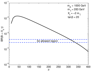
Fig. 16: $\mathcal{B}(B\rightarrow X_{s}\gamma)$ versus $\mu$ with stop soft masses $m_{\tilde{t}}\equiv m_{\tilde{t}_{L}}=m_{\tilde{t}_{R}}=283$ GeV, and natural maximal stop mixing ($X_{t}/m_{\tilde{t}}=-2$). All squark, slepton, and gaugino soft mass parameters are equal to the stop soft masses, $m_{t}=173$ GeV, $m_{A}=1000$ GeV, $\tan\beta=20$, and all the soft trilinear couplings are equal to $A_{t}=X_{t}+\mu\cot\beta$.

4.3 Constraints from $B_{s}\rightarrow\mu^{+}\mu^{-}$

The decay $B_{s}\rightarrow\mu^{+}\mu^{-}$ has not yet been observed. The SM contribution to this decay is dominated by penguin diagrams involving the $Z$-boson and box diagrams involving the $W$-bosons [46]. (The SM Higgs does contribute to the decay $B_{s}\rightarrow\mu^{+}\mu^{-}$ within the SM, but relative to the dominant contribution it is suppressed by $m_{\mu}m_{b,s}/m_{W}^{2}$, where $m_{\mu}$, $m_{b}$ and $m_{s}$ are the masses of the muon, b-quark and s-quark, respectively, and $m_{W}$ is the mass of the $W$-bosons [47].) The SM contribution to the branching ratio is quite small since it is fourth order in the weak interactions. It is predicted to be

$$\mathcal{B}(B_{s}\rightarrow\mu^{+}\mu^{-})_{\textrm{\tiny{SM}}}=(3.42\pm 0.54)\times 10^{-9}$$ (9)

(see [48] and references therein). This is well below the current experimental bound from the CDF experiment at the Tevatron given by

$$\mathcal{B}(B_{s}\rightarrow\mu^{+}\mu^{-})_{\textrm{\tiny{expt}}}<1.5\times 10^{-7}$$ (10)

at the 90$\%$ confidence level [48].

There are several contributions to the decay $B_{s}\rightarrow\mu^{+}\mu^{-}$ from the additional particles in the MSSM, which we now discuss.

The contributions to the decay $B_{s}\rightarrow\mu^{+}\mu^{-}$ coming only from the MSSM Higgs sector are the same as those found in the 2HDM (II). They can be enhanced by two powers of $\tan\beta$ in the amplitude, which can compensate for the suppression by the muon mass. One can set an approximate bound on $m_{H^{+}}$ assuming this is the only contribution within the MSSM. This bound depends on $\tan\beta$, but for $\tan\beta=50$ one finds an experimentally allowed value for $\mathcal{B}(B_{s}\rightarrow\mu^{+}\mu^{-})$ if $m_{H^{+}}\gtrsim 35$ GeV (see for example [49, 50]). As we discussed in Section 4.2, within the 2HDM (II) the constraint on $\mathcal{B}(B\rightarrow X_{s}\gamma)$ alone forces $m_{H^{+}}$ to be larger than about 350 GeV. Such a large value for $m_{H^{+}}$ guarantees that $\mathcal{B}(B_{s}\rightarrow\mu^{+}\mu^{-})$ is roughly of the same size as the SM result even for quite large $\tan\beta$, so that it alone provides no further constraint on the parameter space within the 2HDM (II) [51].

In the MSSM there are, however, further contributions to the decay $B_{s}\rightarrow\mu^{+}\mu^{-}$ coming from box and penguin diagrams that involve charginos and up-type squarks [50, 51, 52, 53, 54, 55, 56]. The penguin diagrams also contain the neutral Goldstone and Higgs bosons. The self-energy MSSM Higgs penguin diagrams give the leading contribution to $\mathcal{B}(B_{s}\rightarrow\mu^{+}\mu^{-})$ for non-negligible mixing in the stop sector. (In an effective Lagrangian approach these diagrams may be viewed as inducing a non-holomorphic coupling between down-type quarks and the up-type Higgs field.) For large $\tan\beta$, this leading contribution is roughly proportional to $A_{t}^{2}\tan^{6}\beta/m_{A}^{4}$, and can thus be significantly larger than the contributions from the Higgs sector alone. Moreover, this contribution becomes small for very small $\mu$. This contribution does not vanish for degenerate squark masses, nor in the limit of large sparticle masses. Thus, although the branching ratio depends on the size of the stop masses, it is much more sensitive to the size of the Higgs masses, $\tan\beta$ and the amount of stop mixing. A light Higgs sector can give a branching ratio of $B_{s}\rightarrow\mu^{+}\mu^{-}$ that is more than three orders of magnitude above the SM prediction and thus well ruled out, especially if the stop mixing and $\tan\beta$ are large. Moreover, this is the case even for large sparticle masses. Furthermore, such large values for $\mathcal{B}(B_{s}\rightarrow\mu^{+}\mu^{-})$ can be reached within the MSSM without violating any other constraints, including, for example, those on $\mathcal{B}(B\rightarrow X_{s}\gamma)$ [51, 57].

There are further contributions to $\mathcal{B}(B_{s}\rightarrow\mu^{+}\mu^{-})$ which also have a $\tan^{6}\beta/m^{4}_{A}$ behavior, even assuming that the CKM matrix is the only source of flavor violation in the squark sector. These appear if the left-handed up-type soft squark masses of the three generations are not all equal, so that the left-handed down-type soft squark mass-squared matrix has off-diagonal terms. These lead to contributions from loops involving a neutralino or a gluino and a down-type squark [50, 52, 55, 56, 57]. Cancelations between the chargino and gluino contributions can occur and the neutralino contribution, although usually smaller, can then be important (see, for example, [57]).

We estimated the values for $\mathcal{B}(B_{s}\rightarrow\mu^{+}\mu^{-})$ with the program $\mathtt{MicrOMEGA}$ 1.3 [58, 59] and the subroutine $\mathtt{IsaBMM}$ from $\mathtt{IsaTools}$/$\mathtt{IsaJet}$ [55, 60]. We find that the branching ratio of $B_{s}\rightarrow\mu^{+}\mu^{-}$ is well within experimental limits for the region $m_{h}$ $\simeq$ $93$ GeV, $m_{H}\geq 114.4$ GeV and $\cos^{2}(\beta-\alpha)\geq 0.8$ in the case of no (or very little) stop mixing and degenerate squark soft masses. For intermediate mixing with degenerate squark masses near $m_{\tilde{t},\textrm{\tiny{min}}}$, $\mathcal{B}(B_{s}\rightarrow\mu^{+}\mu^{-})$ is consistent with experimental limits for $\tan\beta\lesssim 20-25$. For natural maximal mixing, $\mathcal{B}(B_{s}\rightarrow\mu^{+}\mu^{-})$ is consistent with experimental limits for $\tan\beta\lesssim$ 15. For larger $\tan\beta$, as well as for non-degenerate squark soft masses, a scan over all relevant MSSM parameters is necessary in order to see whether we can find an experimentally consistent value of $\mathcal{B}(B_{s}\rightarrow\mu^{+}\mu^{-})$ for such a light Higgs sector. However, for large stop mixing, it will become increasingly difficult to find a parameter set that gives a branching ratio consistent with experiments as $\tan\beta$ is increased. Of course, this assumes that there are no fortuitous cancelations between the different contributions, and also that there are no other flavor-violating contributions such as from R-parity violating couplings. A scan over the relevant MSSM parameters, even assuming MFV, is beyond the scope of this paper. The reader is referred to the references found in the previous two paragraphs, and especially [45], bearing in mind that the current CDF bound on $\mathcal{B}(B_{s}\rightarrow\mu^{+}\mu^{-})$, equation (10), is stronger than the one used in these references.

In the Higgs decoupling limit, the dominant flavor-violating effects involving loops of neutral Higgs bosons decouple, and these large contributions to $B_{s}\rightarrow\mu^{+}\mu^{-}$ become negligible. Using $\mathtt{MicrOMEGA}$ 1.3, one may explicitly check that the decay $B_{s}\rightarrow\mu^{+}\mu^{-}$ does not provide stronger constraints on the stop masses than do the LEP Higgs bounds in the decoupling limit found in Section 3.1.

5 Implications for Electroweak Symmetry
Breaking

In Section 3, we presented lower bounds on the stop masses consistent with the LEP Higgs bounds, and in Section 4, we discussed whether the electroweak $S$- and $T$-parameter and the decays $B\rightarrow X_{s}\gamma$ and $B_{s}\rightarrow\mu^{+}\mu^{-}$ indirectly put further constraints on the Higgs and/or stop sector. In this section, we look at the implications for electroweak symmetry breaking.

The mechanism of radiative electroweak symmetry breaking arises rather naturally in supersymmetric extensions of the Standard Model [61, 62, 63]. Because of the large top Yukawa coupling, quantum fluctuations of the stop squarks significantly modify the up-type Higgs potential, as studied numerically for the physical Higgs boson mass in the previous sections. The leading effect, however, is a tachyonic contribution to the up-type Higgs soft supersymmetry breaking Lagrangian mass. Over much of parameter space this tachyonic contribution is sufficient to result in a stop squark quantum fluctuation-induced phase transition for the Higgs fields, which is generally referred to as radiative electroweak symmetry breaking.

The leading quantum contribution to the up-type Higgs soft mass comes from renormalization group evolution below the supersymmetry breaking messenger scale. The one-loop $\beta$-function for the up-type Higgs soft mass-squared is, neglecting effects proportional to gauge couplings,

$$16\pi^{2}\beta_{m^{2}_{H_{u}}}\simeq 6\lambda_{t}^{2}(m^{2}_{H_{u}}+m_{\tilde{t}_{L}}^{2}+m_{\tilde{t}_{R}}^{2}+|A_{t}|^{2})$$ (11)

The light Higgs mass bounds require rather large stop masses and/or stop mixing, where the stop soft trilinear coupling is related to the mixing parameter by $A_{t}=X_{t}+\mu\cot\beta$. This implies that the stop contributions to the $\beta$-function in (11) proportional to the combination $(m_{\tilde{t}_{L}}^{2}+m_{\tilde{t}_{R}}^{2}+|A_{t}|^{2})$ are also sizeable, at least at the low scale. Moreover, for generic parameters this combination remains sizeable over the entire renormalization group trajectory up to the messenger scale. For generic messenger scale values of the up-type Higgs soft mass squared, $m^{2}_{H_{u}}$, the large value of the combination $(m_{\tilde{t}_{L}}^{2}+m_{\tilde{t}_{R}}^{2}+|A_{t}|^{2})$, along with the sizeable coefficient in the $\beta$-function (11), then imply that $m^{2}_{H_{u}}$ evolves relatively rapidly under renormalization group evolution.

This evolution is towards tachyonic values of $m^{2}_{H_{u}}$ which reduce the magnitude of the $\beta$-function (11). For running into the deep infrared, the up-type Higgs mass squared would be driven to values near the zero of the $\beta$-function (11) for which

$$m^{2}_{H_{u}}\simeq-(m_{\tilde{t}_{L}}^{2}+m_{\tilde{t}_{R}}^{2}+|A_{t}|^{2}).$$ (12)

Although this relation is not strictly obtained with finite running, the up-type Higgs mass squared can approach this value for very high messenger scale. In Table 1, we show the minimum allowed values of the combination $(m_{\tilde{t}_{L}}^{2}+m_{\tilde{t}_{R}}^{2}+|A_{t}|^{2})^{1/2}$ deduced from the results of section 3.1 consistent with $m_{h}\geq 114.4$ GeV in the Higgs decoupling limit for large $\tan\beta$. The minimum allowed values increase with decreasing $\tan\beta$.

$X_{t}/m_{\tilde{t}}$	$m_{t}=168$ GeV	$m_{t}=173$ GeV	$m_{t}=178$ GeV
0	3630	1780	1240
-1	1460	1000	770
-2	680	690	710

Table 1: Minimum allowed values of the combination $(m_{\tilde{t}_{L}}^{2}+m_{\tilde{t}_{R}}^{2}+|A_{t}|^{2})^{1/2}$ consistent with a physical Higgs boson mass of $m_{h}\geq 114.4$ GeV in the Higgs decoupling limit for large $\tan\beta$, taking into account only the LEP Higgs sector bounds. The minimum allowed values increase with decreasing $\tan\beta$.

The full Lagrangian mass squared for the up-type Higgs is a sum of the soft mass squared and square of the superpotential Higgs mass, $m^{2}=m^{2}_{H_{u}}+|\mu|^{2}$. To leading order in $1/\tan^{2}\beta$, and ignoring the finite quantum corrections to the Higgs potential which are not of qualitative importance for the present discussion, this is equal to minus half the $Z$-boson mass squared in the ground state with broken electroweak symmetry

$$\frac{1}{2}m_{Z}^{2}\simeq-(m^{2}_{H_{u}}+|\mu|^{2}).$$ (13)

For $m^{2}_{H_{u}}$ near the zero of its $\beta$-function given by (12), the bounds given in Table 1 imply that obtaining the observed value of the $Z$-boson mass, $m_{Z}\simeq 91$ GeV, requires a rather sensitive cancelation between the up-type Higgs soft mass and $\mu$-parameter. The numerical magnitude of this tuning (which has come to be known as the supersymmetric little hierarchy problem) is apparent in the numerical data in Table 1, at least for regions of parameter space which are driven under renormalization group flow to near the zero of the $\beta$-function (11).

The minimum allowed value of the combination $(m_{\tilde{t}_{L}}^{2}+m_{\tilde{t}_{R}}^{2}+|A_{t}|^{2})$ for a given lower limit on the Higgs mass decreases with increasing stop mixing. This may be understood from the leading expression for the quantum corrected Higgs mass given in equation (5). For no stop mixing, $X_{t}=0$, the leading correction to the Higgs mass squared comes only from renormalization group running of the Higgs quartic coupling below the stop mass scale, and is therefore proportional to $\ln(m^{2}_{\tilde{t}}/m_{t}^{2})$. A linear increase in the Higgs mass squared in this case requires an exponential increase in $m_{\tilde{t}}$. However, the stop mixing correction to the Higgs mass squared with $X_{t}\neq 0$ comes from a finite threshold correction to the Higgs quartic coupling at the stop mass scale and is independent of $m_{\tilde{t}}$ for fixed $X_{t}/m_{\tilde{t}}$. In this case a linear increase in the Higgs mass squared only requires a linear increase in $(X_{t}/m_{\tilde{t}})^{2}$. So increasing stop mixing allows exponentially lighter stop masses in order to obtain a given Higgs mass. While such a decrease clearly reduces the soft stop mass contributions to $\beta_{m^{2}_{H_{u}}}$ [18, 64] this is partially offset by an increase in the mixing contribution from the stop trilinear coupling. From the data in Table 1, it is clear that large stop mixing can decrease the magnitude of $\beta_{m^{2}_{H_{u}}}$ (11) by up to a factor of a few depending on the top mass. However, the magnitude of the total stop contribution including mixing is still quite sizeable for a Higgs mass bound of $m_{h}\geq 114.4$ GeV. So large stop mixing alone cannot appreciably ameliorate the tuning of supersymmetric electroweak symmetry breaking or satisfactorily solve the supersymmetric little hierarchy problem.

This conclusion essentially remains unchanged for a physical Higgs boson mass of $m_{h}\simeq 93$ GeV with $\cos^{2}(\beta-\alpha)\geq 0.8$ and $m_{H}\geq 114.4$ GeV, as seen from the numerical results in Section 3.3. In general, one should bear in mind that indirect constraints on new physics, especially from $\mathcal{B}(B_{s}\rightarrow\mu^{+}\mu^{-})$, severely restrict the allowed MSSM parameter space for $m_{h}\simeq 93$ GeV (see Section 4). However, for less than maximal stop mixing, the stop masses can be somewhat smaller for moderate $\tan\beta$ near the Higgs non-decoupling limit than in the Higgs decoupling limit (see also [9]). The combination $(m_{\tilde{t}_{L}}^{2}+m_{\tilde{t}_{R}}^{2}+|A_{t}|^{2})^{1/2}$ is in fact the smallest in the Higgs non-decoupling region near intermediate values for the stop mixing and for $\tan\beta$ near 10. It reaches as low as about 650 for $m_{t}=178$, $\tan\beta=10.5$, $X_{t}=-m_{\tilde{t}}$, and gaugino masses equal to $m_{\tilde{t}}$. It can be decreased slightly further by setting the bino and wino masses to smaller values. (For maximal stop mixing, the combination is actually larger since here the Tevatron bound on the lighter stop mass forces the stop soft masses to be larger than required from the LEP Higgs bounds alone.) The combination always remains sizeable though, and thus the tuning of electroweak symmetry breaking cannot be ameliorated by much in the $m_{h}\simeq 93$ GeV region.

6 Conclusions

The dominant radiative corrections to the tree-level CP-even Higgs mass matrix, which determines $m_{h}$ and $m_{H}$, come from loops involving the top quark and stop squarks, with larger stop masses implying larger radiative corrections. In this paper, we presented lower bounds on the stop masses consistent with the LEP Higgs bounds in two different regions in the MSSM Higgs parameter space. The one region is the Higgs decoupling limit, in which the bound on the mass of the lighter Higgs is equal to the bound on the SM Higgs, $m_{h}\geq 114.4$ GeV. The other region is near the Higgs “non-decoupling” limit with $m_{h}\simeq 93$ GeV in which the Higgs sector is required to be light. In the latter region, there are two additional constraints. One is on the mass of the heavier Higgs, which now behaves like the SM Higgs, i.e. $m_{H}\gtrsim 114.4$ GeV. The other constraint is on size of the coupling of the lighter Higgs to two $Z$ bosons which is controlled by the parameter $\sin^{2}(\beta-\alpha)$ and here needs to be less than about 0.2 (i.e. $\cos^{2}(\beta-\alpha)\gtrsim 0.8$) for the lighter Higgs to have escaped detection at LEP. We denote the lower bounds on the stop masses consistent with the LEP Higgs bounds by $m_{\tilde{t},\textrm{\tiny{min}}}$.

We presented $m_{\tilde{t},\textrm{\tiny{min}}}$ as a function of $\tan\beta$ in both these regions in the Higgs parameter space for a variety of MSSM parameter choices. In particular, we further elucidated the importance of the top mass and stop mixing, and investigated numerically how larger top masses and more stop mixing allow for substantially smaller values of $m_{\tilde{t},\textrm{\tiny{min}}}$. We also showed numerically how larger gaugino masses and larger values of $\mu$ increase $m_{\tilde{t},\textrm{\tiny{min}}}$. Moreover, we saw how much $m_{\tilde{t},\textrm{\tiny{min}}}$ increases if $\mu$ is negative compared to $\mu$ positive if both $\tan\beta$ and the magnitude of $\mu$ are large. In the non-decoupling region, we discussed how the constraints on $\cos^{2}(\beta-\alpha)$ and on $m_{H}$ lead to increased values for $m_{\tilde{t},\textrm{\tiny{min}}}$.

We also considered how $m_{\tilde{t},\textrm{\tiny{min}}}$ changes as a function of $m_{h}$. Since $A_{t}$ and $M_{3}$ most naturally have the opposite sign at low scales due to renormalization group running, a negative value of $A_{t}$ is more natural in a convention where $M_{3}$ is positive. For negative $A_{t}$ and stop masses less than a few TeV, the upper bound of $m_{h}$ in the MSSM is around 131 GeV.

We demonstrated that the two regions in the Higgs parameter space have roughly the same $m_{\tilde{t},\textrm{\tiny{min}}}$ if $\tan\beta$ is large. For moderate values of $\tan\beta$ and non-maximal stop mixing, $m_{\tilde{t},\textrm{\tiny{min}}}$ is larger in the Higgs decoupling region than in the Higgs non-decoupling region. As $\tan\beta$ decreases, however, $m_{\tilde{t},\textrm{\tiny{min}}}$ is larger in the Higgs non-decoupling region than in the Higgs decoupling region.

We also considered additional constraints from the electroweak $S$- and $T$-parameter and the decays $B\to X_{s}\gamma$ and $B_{s}\to\mu^{+}\mu^{-}$, which also constrain the Higgs and/or stop sector.

The main contribution to the $T$-parameter within the MSSM usually comes from the stop/sbottom doublet and, for a given set of parameters, is larger for larger stop (and sbottom) mixing as well as for smaller stop and sbottom masses. We found that the value of the $T$-parameter is well within its 2$\sigma$ bound for stop masses equal to $m_{\tilde{t},\textrm{\tiny{min}}}$. In fact, only for maximal stop mixing do we find small enough values for $m_{\tilde{t},\textrm{\tiny{min}}}$ that give a contribution to the $T$-parameter that does not also fall within its 1$\sigma$ bound. For such large stop mixing one must then increase the stop masses by a small amount above $m_{\tilde{t},\textrm{\tiny{min}}}$ to also satisfy the 1$\sigma$ bound on the $T$-parameter.

We found that the contribution to the $S$-parameter is not large, and that the $S$-parameter therefore does not provide an additional constraint on the stop masses.

The indirect constraint on $\mathcal{B}(B\rightarrow X_{s}\gamma)$ in many cases does not provide an additional constraint on the stop masses. In the Higgs non-decoupling region for $m_{h}\simeq 93$ GeV, the Higgs sector is required to be light, and the charged Higgs contribution to $B\rightarrow X_{s}\gamma$ is large. The charged Higgs contribution can usually be canceled by the chargino-stop contribution through a judicious choice of the chargino mass. However, for vanishing stop mixing and assuming degenerate stop soft masses, $m_{\tilde{t},\textrm{\tiny{min}}}$ is so large that the chargino-stop contribution is too small to cancel the charged Higgs contribution. For vanishing stop mixing, we therefore require non-degenerate stop soft masses with one light stop so that the chargino-stop contribution can be large enough to give an experimentally consistent value for $\mathcal{B}(B\rightarrow X_{s}\gamma)$ (the other stop must then be very heavy so that the LEP Higgs constraints are satisfied). In the Higgs decoupling limit, the charged Higgs contribution vanishes. We find no further constraint on the stop masses. Even for large stop mixing, for which $m_{\tilde{t},\textrm{\tiny{min}}}$ can be very small, one can always obtain an experimentally consistent value for $\mathcal{B}(B\rightarrow X_{s}\gamma)$ by adjusting the chargino mass.

The main contributions to the flavor-violating decay $B_{s}\rightarrow\mu^{+}\mu^{-}$ come from flavor violating Higgs couplings, and these decouple in the Higgs decoupling limit. Thus, the indirect constraint on $\mathcal{B}(B_{s}\rightarrow\mu^{+}\mu^{-})$ is only important in the Higgs non-decoupling region. In this region, however, it is able to severely restrict the allowed parameter space, since the flavor violation does not decouple in the limit of large sparticle masses. In fact, the region for such a light Higgs sector is ruled out if stop mixing and $\tan\beta$ are large, unless there are fortuitous cancelations amongst the various contributions, or there are additional flavor-violating contributions from, for example, R-parity violating couplings that cancel these contributions.

We note that we did not consider the constraint on the anomalous magnetic moment of the muon, $(g-2)_{\mu}$, since it decouples in the limit of large sneutrino and smuon masses. It alone is thus unable to directly provide a further constraint on the Higgs sector or on the stop masses.

Lastly, we discussed the implications of our numerical analysis for electroweak symmetry breaking. Large stop mixing generically decreases the tuning of supersymmetric electroweak symmetry breaking, but is unable to do so sufficiently to solve the supersymmetric little hierarchy problem. Moreover, the tuning can be ameliorated only slightly in the $m_{h}\simeq 93$ GeV region compared to the $m_{h}\geq 114.4$ GeV region (for intermediate values of the stop mixing and moderate values of $\tan\beta$), and thus the supersymmetric little hierarchy problem cannot be satisfactorily solved in either of the two regions.

Acknowledgements

I would like to thank my advisor S. Thomas for suggesting this project and for his support and guidance throughout. I would also like to thank S. Heinemeyer for helpful email exchanges about $\mathtt{FeynHiggs}$. It is a pleasure to further acknowledge useful conversations with J.F. Fortin, D.E. Kaplan, A. Lath, N. Sehgal, and N. Weiner, as well as R. Dermíšek who pointed out two relevant references. I also want to thank J. Shelton for reading the manuscript and providing many helpful suggestions. This research is supported by a Graduate Assistantship from the Department of Physics and Astronomy at Rutgers University.

Appendix A Mixing in the Two Doublet Higgs Sector

A Higgs sector with electroweak symmetry broken to electromagnetism,
$SU(2)_{L}\times U(1)_{Y}\rightarrow U(1)_{Q}$, by two $SU(2)_{L}$ doublets, $H_{u}$ and $H_{d}$, with hypercharge $Y=\pm 1$ respectively, has two physical scalars, $h$ and $H$, a pseudoscalar, $A$, and a charged scalar, $H^{\pm}$. The couplings of the scalar mass eigenstates, $h$ and $H$, to the gauge bosons are determined by the associated amplitudes of the neutral components of the gauge eigenstate doublets, $H_{u}^{0}$ and $H_{d}^{0}$. It is instructive to consider various vectors in the ${\rm Re}(H_{d}^{0})-{\rm Re}(H_{u}^{0})$ plane in order to describe these couplings and the relationship between the mass and gauge interaction eigenstates.

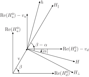
Fig. 17: Relationship between the ${\rm Re}(H_{u})-{\rm Re}(H_{d})$ and $H_{\|}-H_{\bot}$ bases and $h-H$ mass eigenstates for the two doublet Higgs sector.

Electroweak symmetry is broken by the expectation values $\langle{\rm Re}(H_{u}^{0})\rangle=v_{u}$ and $\langle{\rm Re}(H_{d}^{0})\rangle=v_{d}$. These expectation values define a vector in the ${\rm Re}(H_{d}^{0})-{\rm Re}(H_{u}^{0})$ plane with an angle $\beta$ defined by $\tan\beta=v_{u}/v_{d}$ as indicated in Fig. 17. The two physical neutral CP-even scalar mass eigenstates are fluctuations about the expectation value in this plane and are related by a rotation to the gauge eigenstates conventionally defined by an angle $\alpha$ as [66]

$$\left(\begin{array}[]{c}H\\ h\end{array}\right)=\sqrt{2}\left(\begin{array}[]{cc}\cos\alpha&\sin\alpha\\ -\sin\alpha&\cos\alpha\end{array}\right)\left(\begin{array}[]{c}{\rm Re}(H_{d}^{0})-v_{d}\\ {\rm Re}(H_{u}^{0})-v_{u}\end{array}\right)$$ (14)

Vectors in the ${\rm Re}(H_{d}^{0})-{\rm Re}(H_{u}^{0})$ plane which are parallel and perpendicular, $H_{\|}$ and $H_{\bot}$, to the expectation value vector may also be defined as indicated in Fig. 17

$$\left(\begin{array}[]{c}H_{\bot}\\ H_{\|}\end{array}\right)=\sqrt{2}\left(\begin{array}[]{cc}\sin\beta&-\cos\beta\\ \cos\beta&\sin\beta\end{array}\right)\left(\begin{array}[]{c}{\rm Re}(H_{d}^{0})-v_{d}\\ {\rm Re}(H_{u}^{0})-v_{u}\end{array}\right),$$ (15)

see also [9]. The physical mass eigenstates are related to these by a rotation

$$\left(\begin{array}[]{c}H\\ h\end{array}\right)=\left(\begin{array}[]{cc}\sin(\beta-\alpha)&\cos(\beta-\alpha)\\ -\cos(\beta-\alpha)&\sin(\beta-\alpha)\end{array}\right)\left(\begin{array}[]{c}H_{\bot}\\ H_{\|}\end{array}\right).$$ (16)

The neutral Goldstone pseudoscalar boson, $G$, which is eaten by the $Z$-boson is by definition the imaginary part of the linear combination of the components of the neutral Higgs doublets which are aligned with the expectation value, and the physical pseudoscalar Higgs boson, $A$, is the perpendicular combination

$$\begin{array}[]{c}A={\rm Im}(H_{\bot})\\ G={\rm Im}(H_{\|})\end{array}.$$ (17)

These states are related to the gauge eigenstates through a rotation by the angle $\beta$

$$\left(\begin{array}[]{c}A\\ G\end{array}\right)=\sqrt{2}\left(\begin{array}[]{cc}-\sin\beta&\cos\beta\\ \cos\beta&\sin\beta\end{array}\right)\left(\begin{array}[]{c}{\rm Im}(H_{d}^{0})\\ {\rm Im}(H_{u}^{0})\end{array}\right).$$ (18)

The charged Goldstone bosons, $G^{\pm}$, and the charged Higgs mass eigenstates, $H^{\pm}$, are defined similarly as

$$\begin{array}[]{c}H^{\pm}={\rm Im}(H_{\bot}^{\pm})\\ G^{\pm}={\rm Im}(H_{\|}^{\pm})\end{array},$$ (19)

where $H_{\bot}^{\pm}$ and $H_{\bot}^{\pm}$ are defined in analogy with equation (15).

We may consider Higgs decoupling limits of the two doublet Higgs sector in which $m_{H},m_{A},m_{H^{\pm}}\gg m_{h}$ so that only a single light Higgs doublet remains in the low energy theory. A particular decoupling limit is one for which the physical mass eigenstate of the light Higgs doublet is aligned with the expectation value vector so that $H_{\|}$ is the single Higgs doublet of the low energy theory and $H_{\bot}$ contains the heavy mass eigenstates. This is the unique decoupling limit available to the the tree-level Higgs potential of the MSSM, although other misaligned decoupling limits may be realized for more general two doublet potentials. In the aligned decoupling limit $h=H_{\|}$ with $\sin(\beta-\alpha)=1$ and $\cos(\beta-\alpha)=0$.

The couplings of physical Higgs bosons to gauge bosons arise from the gauge kinetic terms of the Higgs fields

$$(D_{\mu}H_{u})^{*}D^{\mu}H_{u}+(D_{\mu}H_{d})^{*}D^{\mu}H_{d}$$ (20)

where $D_{\mu}=\partial_{\mu}+ig^{\prime}\frac{1}{2}YB_{\mu}+igT^{a}W^{a}_{\mu}$ is the covariant derivative including the $SU(2)_{L}\times U(1)_{Y}$ gauge connections $W_{\mu}^{a}$ and $B_{\mu}$. A coupling of two gauge bosons to a single physical Higgs boson arises from (20) with a gauge field in each covariant derivative, a physical Higgs boson in one Higgs field, and an expectation value in the other Higgs field. In terms of the $H_{\|}-H_{\bot}$ basis these couplings are particularly simple. Since it is only $H_{\|}$ which is parallel to the expectation value, only this component appears in these couplings

$$(D_{\mu}v)^{*}D^{\mu}H_{\|}+(D_{\mu}H_{\|})^{*}D^{\mu}v,$$ (21)

where of course $D_{\mu}v$ contains only gauge field couplings since $\partial_{\mu}v=0$. In terms of the physical gauge bosons, the couplings in (21) give rise to $WWH_{\|}$ and $ZZH_{\|}$ interactions. In terms of the physical Higgs scalar eigenstates $h$ and $H$ related to $H_{\|}$ in (16) these couplings give interactions $WWh$ and $ZZh$ proportional to $\sin(\beta-\alpha)$ and interactions $WWH$ and $ZZH$ proportional to $\cos(\beta-\alpha)$. In the Higgs aligned decoupling limit the latter interactions vanish since $H=H_{\bot}$ in this limit with $\cos(\beta-\alpha)=0$. Note that there are no interactions of two gauge bosons with a single charged Higgs boson of the form $W^{\pm}ZH^{\mp}$, since from (19) the physical charged Higgs boson resides in $H_{\bot}$, while from (21) these type of interactions arise only for $H_{\|}$. This result generalizes to any number of Higgs doublets.

A coupling of a single gauge boson to two physical Higgs bosons arises from (20) with a single gauge field in one of the covariant derivatives, physical Higgs bosons in each Higgs field, and a derivative acting on one of the Higgs fields

$$(D_{\mu}H^{*})\partial^{\mu}H+(\partial_{\mu}H)^{*}D^{\mu}H$$ (22)

where the covariant derivatives $D_{\mu}$ are again understood to only contain gauge fields here. This subset of couplings represents the Higgs current coupling to a single gauge boson, and therefore must contain at least one imaginary component of a Higgs field. Now from equations (17) and (19) the imaginary components of the Higgs fields appear in the physical mass eigenstates only through $H_{\bot}$. So the couplings (22) to physical mass eigenstates are contained in

$$(D_{\mu}H_{\bot})^{*}\partial^{\mu}H_{\bot}+(\partial_{\mu}H_{\bot})^{*}D^{\mu}H_{\bot}$$ (23)

In terms of the physical $Z$ gauge boson these couplings give rise to $ZH_{\bot}H_{\bot}$ interactions. In terms of the physical eigenstates $h$ and $H$ related to $H_{\bot}$ in (16), these couplings give the interaction $ZAH$ proportional to $\sin(\beta-\alpha)$ and $ZAh$ proportional to $\cos(\beta-\alpha)$. In the Higgs aligned decoupling limit the latter interaction vanishes since $h=H_{\|}$ in this limit with $\cos(\beta-\alpha)=0$.

Appendix B Quasi-Fixed Point for the Stop Trilinear
Coupling $A_{t}$

The MSSM has a number of quasi-fixed points for various couplings that make a relation in the low energy theory between them and other parameters quite natural. These couplings include the top Yukawa and top trilinear coupling. Consider first the so called Pendleton-Ross quasi-fixed point for the top Yukawa [67]. The one-loop $\beta$-functions for the top Yukawa $\lambda_{t}$ and $SU(3)_{C}$ gauge coupling $g_{3}$ in the MSSM are

$$16\pi^{2}\beta_{\lambda_{t}}=\lambda_{t}\big{(}6\lambda_{t}^{2}-\frac{16}{3}g_{3}^{2}\big{)}$$ (24)

$$16\pi^{2}\beta_{g_{3}}=-3~{}g_{3}^{3}$$ (25)

where $SU(2)_{L}$ and $U(1)_{Y}$ gauge interactions have been neglected in $\beta_{\lambda_{t}}$. These $\beta$-functions give a one-loop $\beta$-function for the logarithm of the ratio of couplings of

$$16\pi^{2}\beta_{\ln(\lambda_{t}/g_{3})}=6\lambda_{t}^{2}-\frac{7}{3}g_{3}^{2}.$$ (26)

Vanishing of this $\beta$-function implies that the ratio of the top Yukawa to $SU(3)_{C}$ gauge coupling, $\lambda_{t}/g_{3}$, is independent of renormalization group scale at one-loop. Since $\beta_{g_{3}}$ does not vanish at one-loop, $g_{3}$ is renormalization scale dependent. So the vanishing of $\beta_{\ln(\lambda_{t}/g_{3})}$ defines a quasi-fixed point for $\lambda_{t}$ rather than a scale-independent fixed-point relation. With the above approximations the Pendleton-Ross quasi-fixed point in the MSSM occurs for

$$\lambda_{t}^{2}=\frac{7}{18}g_{3}^{2}.$$ (27)

Since $\beta_{g_{3}}$ is independent of $\lambda_{t}$ at one-loop, and the coefficient of the $\lambda_{t}^{2}$ term in $\beta_{\ln(\lambda_{t}/g_{3})}$ is positive, this quasi-fixed point is attractive for $\lambda_{t}/g_{3}$ both above and below the quasi-fixed point value. Moreover, since $\beta_{\lambda_{t}}$ is cubic in $\lambda_{t}$, it is very strongly attractive from above.

The top trilinear coupling and gluino mass have a similar quasi-fixed point relation [68, 69]. The one-loop $\beta$-functions for the top trilinear coupling, $A_{t}$, and gluino mass, $M_{3}$, are

$$16\pi^{2}\beta_{A_{t}}=12\lambda_{t}^{2}A_{t}+\frac{32}{3}g_{3}^{2}M_{3}$$ (28)

$$16\pi^{2}\beta_{M_{3}}=-2g_{3}^{2}M_{3}$$ (29)

where $SU(2)_{L}$ and $U(1)_{Y}$ gauge interactions have been neglected in $\beta_{A_{t}}$. Adding these $\beta$-functions gives

$$16\pi^{2}\beta_{(A_{t}+M_{3})}=12\lambda_{t}^{2}A_{t}+\frac{14}{3}g_{3}^{2}M_{3}.$$ (30)

At the Pendleton-Ross quasi-fixed point (27) for the top Yukawa in the MSSM this reduces to

$$16\pi^{2}\beta_{(A_{t}+M_{3})}={14\over 3}g_{3}^{2}\left(A_{t}+M_{3}\right).$$ (31)

The vanishing of $\beta_{A_{t}+M_{3}}$ again defines a quasi-fixed point for $A_{t}$ rather than a scale independent fixed point relation. With the above approximations at the Pendleton-Ross quasi-fixed point, the top trilinear then has a quasi-fixed point of

$$A_{t}=-M_{3}.$$ (32)

Since the coefficient of $\beta_{A_{t}+M_{3}}$ is positive, this quasi-fixed point is attractive. Moreover, since it is proportional to $g_{3}^{2}$ with a sizeable coefficient it is rather strongly attractive. Because of this it is most natural for $A_{t}$ and $M_{3}$ to have opposite sign and be comparable in magnitude at low scales due to renormalization group evolution. This conclusion is rather insensitive to messenger scale boundary conditions for $A_{t}$, at least for large enough messenger scales.

References

- [1] ALEPH, DELPHI, L3 and OPAL Collaboration, The LEP Working Group for Higgs Boson Searches, “Search for neutral MSSM Higgs bosons at LEP,” hep-ex/0602042.
- [2] The LEP Working Group for Higgs boson searches: Barate et al., “Search for the standard model Higgs boson at LEP,” Phys. Lett. B565 (2003) 61–75, hep-ex/0306033.
- [3] The LEP Working Group for Higgs boson searches, “Searches for invisible Higgs bosons: Preliminary combined results using LEP data collected at energies up to 209 GeV,” hep-ex/0107032.
- [4] A. Belyaev, Q.-H. Cao, D. Nomura, K. Tobe, and C. P. Yuan, “Light MSSM Higgs boson scenario and its test at hadron colliders,” hep-ph/0609079.
- [5] Y. Okada, M. Yamaguchi, and T. Yanagida, “Upper bound of the lightest Higgs boson mass in the minimal supersymmetric standard model,” Prog. Theor. Phys. 85 (1991) 1–6.
- [6] J. R. Ellis, G. Ridolfi, and F. Zwirner, “Radiative corrections to the masses of supersymmetric Higgs bosons,” Phys. Lett. B257 (1991) 83–91.
- [7] H. E. Haber and R. Hempfling, “Can the mass of the lightest Higgs boson of the minimal supersymmetric model be larger than m(Z)?,” Phys. Rev. Lett. 66 (1991) 1815–1818.
- [8] H. E. Haber, R. Hempfling, and A. H. Hoang, “Approximating the radiatively corrected Higgs mass in the minimal supersymmetric model,” Z. Phys. C75 (1997) 539–554, hep-ph/9609331.
- [9] S. G. Kim et al., “A solution for little hierarchy problem and b s gamma,” Phys. Rev. D74 (2006) 115016, hep-ph/0609076.
- [10] W.-M. Yao et al., “Review of Particle Physics,” Journal of Physics G 33 (2006) 1+.
- [11] S. Heinemeyer, W. Hollik, and G. Weiglein, “FeynHiggs: A program for the calculation of the masses of the neutral CP-even Higgs bosons in the MSSM,” Comput. Phys. Commun. 124 (2000) 76–89, hep-ph/9812320.
- [12] S. Heinemeyer, W. Hollik, and G. Weiglein, “The masses of the neutral CP-even Higgs bosons in the MSSM: Accurate analysis at the two-loop level,” Eur. Phys. J. C9 (1999) 343–366, hep-ph/9812472.
- [13] G. Degrassi, S. Heinemeyer, W. Hollik, P. Slavich, and G. Weiglein, “Towards high-precision predictions for the MSSM Higgs sector,” Eur. Phys. J. C28 (2003) 133–143, hep-ph/0212020.
- [14] M. Frank et al., “The Higgs boson masses and mixings of the complex MSSM in the Feynman-diagrammatic approach,” hep-ph/0611326.
- [15] M. Carena et al., “Reconciling the two-loop diagrammatic and effective field theory computations of the mass of the lightest CP-even Higgs boson in the MSSM,” Nucl. Phys. B580 (2000) 29–57, hep-ph/0001002.
- [16] S. Heinemeyer, “MSSM Higgs physics at higher orders,” hep-ph/0407244.
- [17] S. Heinemeyer, W. Hollik, and G. Weiglein, “The mass of the lightest MSSM Higgs boson: A compact analytical expression at the two-loop level,” Phys. Lett. B455 (1999) 179–191, hep-ph/9903404.
- [18] R. Kitano and Y. Nomura, “Supersymmetry, naturalness, and signatures at the LHC,” Phys. Rev. D73 (2006) 095004, hep-ph/0602096.
- [19] R. Dermisek and I. Low, “Probing the stop sector and the sanity of the MSSM with the Higgs boson at the LHC,” hep-ph/0701235.
- [20] Tevatron Electroweak Working Group, “Combination of CDF and D0 results on the mass of the top quark,” hep-ex/0608032.
- [21] H. E. Haber and R. Hempfling, “The Renormalization group improved Higgs sector of the minimal supersymmetric model,” Phys. Rev. D48 (1993) 4280–4309, hep-ph/9307201.
- [22] M. Carena, S. Heinemeyer, C. E. M. Wagner, and G. Weiglein, “Suggestions for improved benchmark scenarios for Higgs- boson searches at LEP2,” hep-ph/9912223.
- [23] T. Banks, “Supersymmetry and the quark mass matrix,” Nucl. Phys. B303 (1988) 172.
- [24] L. J. Hall, R. Rattazzi, and U. Sarid, “The Top quark mass in supersymmetric SO(10) unification,” Phys. Rev. D50 (1994) 7048–7065, hep-ph/9306309.
- [25] R. Hempfling, “Yukawa coupling unification with supersymmetric threshold corrections,” Phys. Rev. D49 (1994) 6168–6172.
- [26] M. Carena, M. Olechowski, S. Pokorski, and C. E. M. Wagner, “Electroweak symmetry breaking and bottom - top Yukawa unification,” Nucl. Phys. B426 (1994) 269–300, hep-ph/9402253.
- [27] M. Carena, D. Garcia, U. Nierste, and C. E. M. Wagner, “Effective Lagrangian for the anti-t b H+ interaction in the MSSM and charged Higgs phenomenology,” Nucl. Phys. B577 (2000) 88–120, hep-ph/9912516.
- [28] H. Eberl, K. Hidaka, S. Kraml, W. Majerotto, and Y. Yamada, “Improved SUSY QCD corrections to Higgs boson decays into quarks and squarks,” Phys. Rev. D62 (2000) 055006, hep-ph/9912463.
- [29] S. Heinemeyer, W. Hollik, H. Rzehak, and G. Weiglein, “High-precision predictions for the MSSM Higgs sector at O(alpha(b) alpha(s)),” Eur. Phys. J. C39 (2005) 465–481, hep-ph/0411114.
- [30] M. Carena and H. E. Haber, “Higgs boson theory and phenomenology. ((V)),” Prog. Part. Nucl. Phys. 50 (2003) 63–152, hep-ph/0208209.
- [31] J. M. Moreno, D. H. Oaknin, and M. Quiros, “Sphalerons in the MSSM,” Nucl. Phys. B483 (1997) 267–290, hep-ph/9605387.
- [32] M. Carena, S. Mrenna, and C. E. M. Wagner, “The complementarity of LEP, the Tevatron and the LHC in the search for a light MSSM Higgs boson,” Phys. Rev. D62 (2000) 055008, hep-ph/9907422.
- [33] M. E. Peskin and T. Takeuchi, “Estimation of oblique electroweak corrections,” Phys. Rev. D46 (1992) 381–409.
- [34] J. Erler, “Precision electroweak physics,” hep-ph/0604035.
- [35] S. Heinemeyer, W. Hollik, and G. Weiglein, “Electroweak precision observables in the minimal supersymmetric standard model,” Phys. Rept. 425 (2006) 265–368, hep-ph/0412214.
- [36] S. Eidelman et al., “Review of particle physics,” Phys. Lett. B592 (2004) 1.
- [37] T. Inami, C. S. Lim, and A. Yamada, “Radiative correction parameter S in beyond the standard models,” Mod. Phys. Lett. A7 (1992) 2789–2798.
- [38] T. Becher and M. Neubert, “Analysis of Br(B X/s gamma) at NNLO with a cut on photon energy,” Phys. Rev. Lett. 98 (2007) 022003, hep-ph/0610067.
- [39] Heavy Flavor Averaging Group (HFAG), “Averages of b-hadron properties at the end of 2005,” hep-ex/0603003.
- [40] P. Gambino and M. Misiak, “Quark mass effects in anti-B X/s gamma,” Nucl. Phys. B611 (2001) 338–366, hep-ph/0104034.
- [41] T. Hurth, “Present status of inclusive rare B decays,” Rev. Mod. Phys. 75 (2003) 1159–1199, hep-ph/0212304.
- [42] The LEP Working Group for Higgs boson searches, “Search for charged Higgs bosons: Preliminary combined results using LEP data collected at energies up to 209 GeV,” hep-ex/0107031.
- [43] K. Okumura and L. Roszkowski, “Weakened constraints from b s gamma on supersymmetry flavor mixing due to next-to-leading-order corrections,” Phys. Rev. Lett. 92 (2004) 161801.
- [44] M. Drees, “A supersymmetric explanation of the excess of Higgs-like events at LEP,” Phys. Rev. D71 (2005) 115006, hep-ph/0502075.
- [45] D. Hooper and T. Plehn, “Dark matter and collider phenomenology with two light supersymmetric Higgs bosons,” Phys. Rev. D72 (2005) 115005, hep-ph/0506061.
- [46] T. Inami and C. S. Lim, “Effects of superheavy quarks and leptons in low-energy weak processes K(L) mu anti-mu, K+ pi+ neutrino anti-neutrino K0 anti-K0,” Prog. Theor. Phys. 65 (1981) 297.
- [47] B. Grzadkowski and P. Krawczyk, “Higgs particle effects in flavor changing transitions,” Z. Phys. C18 (1983) 43–45.
- [48] CDF Collaboration, A. Abulencia et al., “Search for and decays in collisions with CDF II,” Phys. Rev. Lett. 95 (2005) 221805, hep-ex/0508036.
- [49] H. E. Logan and U. Nierste, “B/s,d l+ l- in a two-Higgs-doublet model,” Nucl. Phys. B586 (2000) 39–55, hep-ph/0004139.
- [50] P. H. Chankowski and L. Slawianowska, “B0/d,s mu- mu+ decay in the MSSM,” Phys. Rev. D63 (2001) 054012, hep-ph/0008046.
- [51] C. Bobeth, T. Ewerth, F. Kruger, and J. Urban, “Analysis of neutral Higgs-boson contributions to the decays anti-B/s l+ l- and anti-B K l+ l-,” Phys. Rev. D64 (2001) 074014, hep-ph/0104284.
- [52] K. S. Babu and C. F. Kolda, “Higgs-mediated B0 mu+ mu- in minimal supersymmetry,” Phys. Rev. Lett. 84 (2000) 228–231, hep-ph/9909476.
- [53] A. J. Buras, P. H. Chankowski, J. Rosiek, and L. Slawianowska, “Delta(M(d,s)), B/(d,s)0 mu+ mu- and B X/s gamma in supersymmetry at large tan(beta),” Nucl. Phys. B659 (2003) 3, hep-ph/0210145.
- [54] A. Dedes and A. Pilaftsis, “Resummed effective Lagrangian for Higgs-mediated FCNC interactions in the CP-violating MSSM,” Phys. Rev. D67 (2003) 015012, hep-ph/0209306.
- [55] J. K. Mizukoshi, X. Tata, and Y. Wang, “Higgs-mediated leptonic decays of B/s and B/d mesons as probes of supersymmetry,” Phys. Rev. D66 (2002) 115003, hep-ph/0208078.
- [56] A. Dedes, “The Higgs penguin and its applications: An overview,” Mod. Phys. Lett. A18 (2003) 2627–2644, hep-ph/0309233.
- [57] C. Bobeth, T. Ewerth, F. Kruger, and J. Urban, “Enhancement of B(anti-B/d mu+ mu-)/B(anti-B/s mu+ mu-) in the MSSM with minimal flavour violation and large tan beta,” Phys. Rev. D66 (2002) 074021, hep-ph/0204225.
- [58] G. Belanger, F. Boudjema, A. Pukhov, and A. Semenov, “MicrOMEGAs: A program for calculating the relic density in the MSSM,” Comput. Phys. Commun. 149 (2002) 103–120, hep-ph/0112278.
- [59] G. Belanger, F. Boudjema, A. Pukhov, and A. Semenov, “MicrOMEGAs: Version 1.3,” Comput. Phys. Commun. 174 (2006) 577–604, hep-ph/0405253.
- [60] F. E. Paige, S. D. Protopopescu, H. Baer, and X. Tata, “ISAJET 7.69: A Monte Carlo event generator for p p, anti-p p, and e+ e- reactions,” hep-ph/0312045.
- [61] L. E. Ibanez and G. G. Ross, “SU(2)-L x U(1) Symmetry Breaking as a Radiative Effect of Supersymmetry Breaking in GUTs,” Phys. Lett. B110 (1982) 215–220.
- [62] J. R. Ellis, D. V. Nanopoulos, and K. Tamvakis, “Grand Unification in Simple Supergravity,” Phys. Lett. B121 (1983) 123.
- [63] L. Alvarez-Gaume, J. Polchinski, and M. B. Wise, “Minimal Low-Energy Supergravity,” Nucl. Phys. B221 (1983) 495.
- [64] G. L. Kane, T. T. Wang, B. D. Nelson, and L.-T. Wang, “Theoretical implications of the LEP Higgs search,” Phys. Rev. D71 (2005) 035006, hep-ph/0407001.
- [65] R. Dermisek and H. D. Kim, “Radiatively generated maximal mixing scenario for the Higgs mass and the least fine tuned minimal supersymmetric standard model,” Phys. Rev. Lett. 96 (2006) 211803, hep-ph/0601036.
- [66] J. F. Gunion, H. E. Haber, G. L. Kane, and S. Dawson, The Higgs Hunter’s Guide. Alan M. Wylde, 1990.
- [67] B. Pendleton and G. G. Ross, “Mass and Mixing Angle Predictions from Infrared Fixed Points,” Phys. Lett. B98 (1981) 291.
- [68] P. M. Ferreira, I. Jack, and D. R. T. Jones, “Infrared soft universality,” Phys. Lett. B357 (1995) 359–364, hep-ph/9506467.
- [69] M. Lanzagorta and G. G. Ross, “Infrared fixed point structure of soft supersymmetry breaking mass terms,” Phys. Lett. B364 (1995) 163–174, hep-ph/9507366.