The radiative decay of the $\Lambda(1405)$ and its two-pole structure

Abstract

We evaluate theoretically the radiative decay widths into $\gamma\Lambda$ and $\gamma\Sigma^{0}$ of the two poles of the $\Lambda(1405)$ found in chiral unitary theories and we find quite different results for each of the two poles. We show that, depending on which reaction is used to measure the $\Lambda(1405)$ radiative decays, one gives more weight to one or the other pole, resulting in quite different shapes in the $\gamma\Lambda(\Sigma^{0})$ invariant mass distributions. Our results for the high-energy pole agree with those of the empirical determination of the $\gamma\Lambda$ and $\gamma\Sigma^{0}$ radiative widths (based on an isobar model fitting of the $K^{-}p$ atom data), which are sometimes referred to as “experimental data”. We have made a detailed study of the $K^{-}p\rightarrow\pi^{0}\gamma\Lambda(\Sigma^{0})$ and $\pi^{-}p\rightarrow K^{0}\gamma\Lambda(\Sigma^{0})$ reactions and have shown that they, indeed, lead to different shapes for the $\gamma\Lambda(\Sigma^{0})$ invariant mass distributions.

1 Introduction

The nature of the $\Lambda(1405)$ has been in dispute since the early days. In most quark-model calculations, it is described as a $p$-state $q^{3}$ baryon with mainly a SU(3) singlet structure Isgur:1978xj . On the other hand, the $\Lambda(1405)$ resonance has long been suggested to be a bound state of the $\bar{K}N$ system, and therefore of $q^{4}\bar{q}$ structure Dalitz:1960du . In recent years, this argument has been strengthened within the unitary extensions of chiral perturbation theory U$\chi$PT Kaiser:1996js ; Oset:1997it ; Oset:2001cn ; Oller:2000fj ; Jido:2003cb ; Garcia-Recio:2002td ; Garcia-Recio:2003ks ; Hyodo:2002pk . A particularly interesting discovery is that the nominal $\Lambda(1405)$ is a superposition of two resonances. This was hinted in Oller:2000fj and studied in detail in Jido:2003cb , where two poles were found on the second Riemann sheet at $1390-i66$ MeV and $1426-i16$ MeV, respectively. More recently, the studies of the $\bar{K}N$ interaction have been extended by including higher order chiral Lagrangians in the kernel of the interaction Borasoy:2005ie ; Oller:2005ig ; Oller:2006jw ; Borasoy:2006sr . The position of the high-energy pole is rather similar in all these works and in Jido:2003cb , but there are variations in the position of the low-energy pole. Nevertheless, the theoretical uncertainties have been studied in Borasoy:2006sr and the results of Ref. Jido:2003cb fit well within them. As first demonstrated in Ref. Jido:2003cb , due to the fact that these two poles couple differently to the coupled channels, different reactions could observe different invariant mass distributions, thus offering the possibility to experimentally test the two-pole prediction. The reactions $\gamma p\rightarrow K^{+}\Lambda(1405)$ and $K^{-}p\rightarrow\Lambda(1405)\gamma$ are shown to be sensitive to the high-energy pole of the $\Lambda(1405)$ and thus the corresponding invariant mass distributions exhibit a peak at $\sim 1420$ MeV Nacher:1998mi ; Nacher:1999ni . On the other hand, the reaction $\pi^{-}p\rightarrow K^{0}\pi\Sigma$ seems to give more weight to the low-energy pole and thus exhibits a peak around $1390$ MeV in the $\pi\Sigma$ invariant mass distributions Hyodo:2003jw . Such a two-pole structure of the $\Lambda(1405)$ has recently been tested by the reaction $K^{-}p\rightarrow\pi^{0}\pi^{0}\Sigma^{0}$ Prakhov:2004an , as demonstrated in Ref. Magas:2005vu .

The electromagnetic transition rates of excited baryons to their respective ground states provide a relatively clean probe of the structure of the baryons. In this respect, we expect that the radiative decay widths of the $\Lambda(1405)$ can offer us some clues on its two-pole structure. However, the radiative decays of the excited hyperon states have very small branching ratios and to date very few electromagnetic transition rates have been measured. Recently, the CLAS collaboration at Jefferson Lab has reported a new measurement of the radiative decay widths of the $\Sigma^{0}(1385)$ and the $\Lambda(1520)$ Taylor:2005zw , which, as argued in Ref. Myhrer:2006hx , suggests that the wave functions of the hyperon ground states should contain sizable components of excited quark states (configuration mixing). As for the $\Lambda(1405)$, there is no direct measurement of its radiative decay widths. Using an isobar model to fit the $K^{-}p$ atom data of Ref. Whitehouse:1989yi , H. Burkhardt and J. Lowe  Burkhardt:1991ms obtained the following numbers:

$$\Gamma_{\Lambda(1405)\rightarrow\gamma\Lambda(1116)}=27\pm 8\,\mbox{keV},$$

$$\Gamma_{\Lambda(1405)\rightarrow\gamma\Sigma^{0}(1193)}=10\pm 4\,\mbox{keV}\quad\mbox{or}\quad 23\pm 7\,\mbox{keV},$$

which are sometimes quoted as “experimental data” in the literature.

On the other hand, as shown in Ref. Lee:1998gt , the U$\chi$PT model of Refs. Oset:1997it ; Oset:2001cn can also describe rather well the $K^{-}p$ atom data of Ref. Whitehouse:1989yi . Therefore, it is truly desirable to calculate the radiative decay width of the $\Lambda(1405)$ within the same framework. This is the main purpose of the present work.

This paper is organized as follows. In Sect. 2 we give a brief description of the chiral unitary coupled channel approach. In Sect. 3 we calculate the radiative decay widths of the $\Lambda(1405)$, discuss how these numbers are closely related to the chiral structure of our approach and compare our predictions with those of other theoretical models. In Sect. 4 we study the reactions $K^{-}p\rightarrow\pi^{0}\gamma\Lambda(\Sigma^{0})$ and $\pi^{-}p\rightarrow K^{0}\gamma\Lambda(\Sigma^{0})$. There we show that while the first reaction stresses the high-energy pole of the $\Lambda(1405)$ in both the $\gamma\Lambda$ and $\gamma\Sigma^{0}$ channels, the second reaction gives more weight to the low-energy pole in the $\gamma\Sigma^{0}$ channel. Conclusions and a brief summary are presented in Sect. 5.

2 Brief description of the two $\Lambda(1405)$ states in the chiral unitary coupled channel approach

In Oset:1997it ; Oset:2001cn ; Oller:2000fj ; Jido:2003cb , the unitary formalism with coupled channels using chiral Lagrangian is exposed. The lowest order chiral Lagrangian for the interaction of the pseudoscalar mesons of the SU(3) octet of the pion with the baryons of the proton octet is used. By picking the terms that contribute to the $MB\rightarrow MB$ amplitude the Lagrangian is given by Oset:1997it :

$$\mathcal{L}=\frac{1}{4f^{2}}\langle\bar{B}i\gamma^{\mu}[\Phi\partial_{\mu}\Phi-\partial_{\mu}\Phi\Phi,B]\rangle,$$ (1)

which, projected over $s$-wave, provides tree level transition amplitudes Oset:2001cn :

$$V_{ij} = -C_{ij}\frac{1}{4f^{2}}(2\sqrt{s}-M_{B_{i}}-M_{B_{j}})$$ (2)

$$\quad\quad\quad\times\left(\frac{M_{B_{i}}+E}{2M_{B_{i}}}\right)^{1/2}\left(\frac{M_{B_{j}}+E^{\prime}}{2M_{B_{j}}}\right)^{1/2},$$

with $E$, $E^{\prime}$ ($M_{B}$) the energies (masses) of the baryons and $C_{ij}$ coefficients tabulated in Oset:1997it . These tree level amplitudes are used as kernel of the Bethe Salpeter equation in coupled channels

$$T=[1-Vg]^{-1}V,$$ (3)

where $V$ appears factorized on shell Oset:1997it ; Oller:2000fj and $g$ is the loop function of a meson and a baryon propagators, regularized by a cut off in Oset:1997it and in dimensional regularization in Oller:2000fj ; Oset:2001cn ; Jido:2003cb .

For the particular case of ${1/2}^{-}$ states (in $MB$ $s$-wave interaction) with strangeness $S=-1$ and zero charge we have ten channels: $K^{-}p$, $\bar{K}^{0}n$, $\pi^{0}\Lambda$, $\pi^{0}\Sigma^{0}$, $\eta\Lambda$, $\eta\Sigma^{0}$, $\pi^{+}\Sigma^{-}$, $\pi^{-}\Sigma^{+}$, $K^{+}\Xi^{-}$, and $K^{0}\Xi^{0}$. The explicit solution of the Bethe Salpeter equation leads to poles in the second Riemann sheet corresponding to resonances. In this sector one finds two poles close to the nominal $\Lambda(1405)$ resonance, and other poles corresponding to the $\Lambda(1670)$ and other $\Sigma$ resonances Oset:2001cn ; Jido:2003cb . The pole position provides the mass and half width (through its imaginary part) and the residues at the pole give the couplings of the resonance to the different channels. These couplings will be needed in what follows to determine the radiative decay widths of the $\Lambda(1405)$. Only one loop function involving these latter couplings will be used, but one has to keep in mind that the resonance couplings used in the evaluation summarize the effect of the multichannel multiple scattering of the different states prior to the final coupling to the photon. Although arguments of gauge invariance require the coupling of the photon to all internal loops of the diagrammatic series of the Bethe Salpeter equation Borasoy:2005zg , such loops involve an $s$-wave and a $p$-wave vertex and vanish in the present case in the large baryon mass limit. In practice, they are negligible for finite masses Doring:2006ub ; Doring:2005bx .

In Table 1 we summarize the pole position and couplings of the two $\Lambda(1405)$ states to the different channels. These will be used in the next section. We omit in the table the neutral channels $\eta\Lambda$, $\eta\Sigma$, and $\pi\Lambda$, which do not contribute to the radiative decay of the $\Lambda(1405)$.

Table 1: The two poles $z_{R}$ of the $\Lambda(1405)$ and the corresponding couplings to different coupled channels. Taken from Ref. Jido:2003cb .

$z_{R}$	$(1390-66i)$		$(1426-16i)$
	$g_{i}$	$|g_{i}|$	$g_{i}$	$|g_{i}|$
$\pi\Sigma$	$-2.5+1.5i$	2.9	$0.42+1.4i$	1.5
$\bar{K}N$	$1.2-1.7i$	2.1	$-2.5-0.94i$	2.7
$K\Xi$	$-0.45+0.41i$	0.61	$0.11+0.33i$	0.35

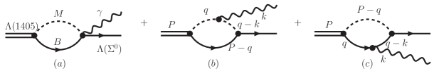
Figure 1: The radiative decay mechanism of the $\Lambda(1405)$, where $MB$ can be any of the four charged channels of the ten coupled channels: $K^{-}p$, $\bar{K}^{0}n$, $\pi^{0}\Lambda$, $\pi^{0}\Sigma^{0}$, $\eta\Lambda$, $\eta\Sigma^{0}$, $\pi^{+}\Sigma^{-}$, $\pi^{-}\Sigma^{+}$, $K^{+}\Xi^{-}$, and $K^{0}\Xi^{0}$.

The model of Ref. Oset:1997it was calibrated using the following threshold branching ratios:

$$\gamma = \frac{\Gamma(K^{-}p\rightarrow\pi^{+}\Sigma^{-})}{\Gamma(K^{-}p\rightarrow\pi^{-}\Sigma^{+})}=2.36\pm 0.04,$$

$$R_{c} = \frac{\Gamma(K^{-}p\rightarrow\mbox{charged particles})}{\Gamma(K^{-}p\rightarrow\mbox{all})}=0.664\pm 0.011,$$

$$R_{n} = \frac{\Gamma(K^{-}p\rightarrow\pi^{0}\Lambda)}{\Gamma(K^{-}p\rightarrow\mbox{all neutral states})}=0.189\pm 0.015.$$

With the same set of parameters, in Ref. Lee:1998gt , the following branching ratios are obtained:

$$B_{K^{-}p\rightarrow\gamma\Lambda} = 1.10\times 10^{-3}\,(0.86\pm 0.16\times 10^{-3}),$$

$$B_{K^{-}p\rightarrow\gamma\Sigma^{0}} = 1.05\times 10^{-3}\,(1.44\pm 0.31\times 10^{-3}),$$

$$R = \frac{B_{K^{-}p\rightarrow\gamma\Lambda}}{B_{K^{-}p\rightarrow\gamma\Sigma^{0}}}=1.04\,(0.4\sim 0.9),$$

which are all in reasonable agreement with the data (shown in the parentheses) Whitehouse:1989yi . We have made use of this model Oset:1997it and have evaluated the branching ratios for other reactions as shown below:

$$R_{\pi^{0}\Lambda} = \frac{\Gamma(K^{-}p\rightarrow\pi^{0}\Lambda)}{\Gamma(K^{-}p\rightarrow\mbox{all})}=0.083\,(0.075),$$

$$R_{\pi^{0}\Sigma^{0}} = \frac{\Gamma(K^{-}p\rightarrow\pi^{0}\Sigma^{0})}{\Gamma(K^{-}p\rightarrow\mbox{all})}=0.293\,(0.261),$$

$$R_{\pi^{+}\Sigma^{-}} = \frac{\Gamma(K^{-}p\rightarrow\pi^{+}\Sigma^{-})}{\Gamma(K^{-}p\rightarrow\mbox{all})}=0.437\,(0.467),$$

$$R_{\pi^{-}\Sigma^{+}} = \frac{\Gamma(K^{-}p\rightarrow\pi^{-}\Sigma^{+})}{\Gamma(K^{-}p\rightarrow\mbox{all})}=0.188\,(0.196),$$

where the numbers in the parentheses are the experimental data Whitehouse:phd . These same data are used to fix the strong coupling constants in the isobar model of Ref. Burkhardt:1991ms to deduce the radiative decay widths of the $\Lambda(1405)$.

As we have seen, with the use of only one cut-off parameter and the lowest-order chiral Lagrangian, one can reproduce fairly well all the low energy data related to the $\Lambda(1405)$, both strong and electromagnetic. In this work, we extend the unitary coupled-channel chiral approach of Refs. Oset:1997it ; Oset:2001cn to investigate the radiative decay widths of the $\Lambda(1405)$. We also study several related reactions to investigate the possibility of experimentally testing the two-pole structure of the $\Lambda(1405)$ and the predictions of the present work.

3 The radiative decay width of the $\Lambda(1405)$

In the picture of the $\Lambda(1405)$ as a dynamically generated resonance from the meson baryon interaction, the coupling of the photon to the resonance proceeds via the coupling to its meson and baryon components. As mentioned in the former section, gauge invariance is preserved in this picture as shown in Ref. Borasoy:2005zg . In practical terms, as shown in Refs. Doring:2006ub ; Doring:2007rz , it means that the mechanisms for the $\Lambda(1405)$ decay into $\gamma\Lambda$ or $\gamma\Sigma^{0}$ are given by the diagrams shown in Fig. 1. The corresponding $t$-matrix elements read

$$-it = \sum_{i}g_{\Lambda(1405)\rightarrow i}(-e)Q_{i}\left[\alpha_{i}\frac{D+F}{2f}+\beta_{i}\frac{D-F}{2f}\right]$$ (4)

$$\times G^{\mu\nu}\sigma_{\mu}\epsilon_{\nu}$$

$$\equiv -ig_{\Lambda(1405)\rightarrow\gamma Y}\vec{\sigma}\cdot\vec{\epsilon}\quad\mbox{with}\quad Y=\Lambda\,\mbox{or}\,\Sigma^{0}$$

with $\sigma^{\mu}=(0,\vec{\sigma})$, where $i$ denotes any of the ten coupled channels $K^{-}p$, $\bar{K}^{0}n$, $\pi^{0}\Lambda$, $\pi^{0}\Sigma^{0}$, $\eta\Lambda$, $\eta\Sigma^{0}$, $\pi^{+}\Sigma^{-}$, $\pi^{-}\Sigma^{+}$, $K^{+}\Xi^{-}$, and $K^{0}\Xi^{0}$. In Eq. (4) $Q_{i}$ is the electric charge of the meson of channel $i$, which is $-1$, 0, 0, 0, 0, 0, 1, $-1$, 1, and 0, respectively, for the ten coupled channels with the order given above. The coupling constants of the $\Lambda(1405)$ to various channels, $g_{\Lambda(1405)\rightarrow i}$, are given in Table 1. It is to be noted that the couplings tabulated in Table 1 are for isospin channels; therefore, appropriate isospin projections are needed when used in Eq. (4). The coupling constants $\alpha_{i}$ and $\beta_{i}$ for the 4 charged channels $K^{-}p$, $\pi^{+}\Sigma^{-}$, $\pi^{-}\Sigma^{+}$, and $K^{+}\Xi^{-}$ are tabulated in Table 2.

Table 2: SU(3) coupling constants defined in Eq. (4) for the channels $K^{-}p$, $\pi^{+}\Sigma^{-}$, $\pi^{-}\Sigma^{+}$, and $K^{+}\Xi^{-}$.

	$K^{-}p$	$\pi^{+}\Sigma^{-}$	$\pi^{-}\Sigma^{+}$	$K^{+}\Xi^{-}$
$\alpha_{MB\rightarrow\Lambda}$	$-\frac{2}{\sqrt{3}}$	$\frac{1}{\sqrt{3}}$	$\frac{1}{\sqrt{3}}$	$\frac{1}{\sqrt{3}}$
$\beta_{MB\rightarrow\Lambda}$	$\frac{1}{\sqrt{3}}$	$\frac{1}{\sqrt{3}}$	$\frac{1}{\sqrt{3}}$	$-\frac{2}{\sqrt{3}}$
$\alpha_{MB\rightarrow\Sigma^{0}}$	0	$1$	$-1$	$1$
$\beta_{MB\rightarrow\Sigma^{0}}$	$1$	$-1$	$1$	0

The loop function $G^{\mu\nu}$ can be easily calculated by employing gauge invariance (see e.g. Refs. Doring:2007rz ; Close:1992ay ; Oller:1998ia ; Marco:1999df ; Roca:2006am ). Since the only external momenta available in the present process are $P$ (the $\Lambda(1405)$ 4-momentum) and $k$ (the photon 4-momentum), the most general amplitude can be written as

$$T=\tilde{T}G^{\mu\nu}\sigma_{\mu}\epsilon_{\nu},$$ (5)

with

$$G^{\mu\nu}=ag^{\mu\nu}+bP^{\mu}P^{\nu}+cP^{\mu}k^{\nu}+dk^{\mu}P^{\nu}+ek^{\mu}k^{\nu}.$$ (6)

Due to the Lorentz condition $\epsilon_{\nu}k^{\nu}=0$, the two terms proportional to $c$ and $e$ vanish. Furthermore, gauge invariance requires that $G^{\mu\nu}k_{\nu}=0$, i.e.

$$ak^{\mu}+bP^{\mu}(P\cdot k)+dk^{\mu}(P\cdot k)=0,$$ (7)

which implies that $b=0$ and

$$a=-d(P\cdot k).$$ (8)

Following these arguments, $T$ only contains the $a$ and $d$ terms. This can be further simplified by noting that in the rest frame of the $\Lambda(1405)$, $\vec{P}=0$, and taking Coulomb gauge for the photon, $\epsilon^{0}=0$, only the $a$ term survives. However, the $a$ term can be more easily computed by employing the relation of Eq. (8). This is due to the fact that on one hand, the $d$ coefficient is found convergent since, due to dimensional reasons, it involves two powers of momentum less in the loop functions than other individual terms, and on the other hand, there are fewer terms which contribute to the $d$ coefficient.

Immediately, one realizes that the diagram $(a)$ shown in Fig. 1 does not contribute to the $d$ term; therefore to calculate $G^{\mu\nu}$, we only need to calculate the diagrams $(b)$ and $(c)$. We first look at the $(b)$ diagram. The corresponding $G^{\mu\nu}$ is explicitly written as

$$G^{\mu\nu}_{(b)} = -i\int\frac{d^{4}q}{(2\pi)^{4}}\frac{1}{q^{2}-m^{2}}\frac{1}{(q-k)^{2}-m^{2}}$$

$$\hskip 14.22636pt\times\frac{2M}{(P-q)^{2}-M^{2}+i\epsilon}(q-k)^{\mu}(2q-k)^{\nu},$$

with $m$ the meson mass and $M$ the baryon mass of the corresponding loop. By employing the Feynman parameterization Peskin:1995ev

$$\frac{1}{abc}=2\int^{1}_{0}dx\,\int^{1-x}_{0}dz\,\frac{1}{[ax+b(1-x-z)+cz]^{3}}$$ (10)

and the following relation Peskin:1995ev

$$\int d^{4}q^{\prime}\frac{1}{(q^{\prime 2}+s+i\epsilon)^{3}}=i\frac{\pi^{2}}{2}\frac{1}{s+i\epsilon},$$ (11)

one can obtain $G^{\mu\nu}_{(b)}\sigma_{\mu}\epsilon_{\nu}$ as

$$G^{\mu\nu}_{(b)}\sigma_{\mu}\epsilon_{\nu} = \frac{2M}{(4\pi)^{2}}\int^{1}_{0}dx\,\int^{1-x}_{0}dz\,\frac{x(1-z)}{s+i\epsilon}(2P\cdot k)\vec{\sigma}\cdot\vec{\epsilon}$$ (12)

$$\equiv G^{b}\vec{\sigma}\cdot\vec{\epsilon}$$

with

$$s=-m^{2}(1-x)+x[P^{2}(1-x)-M^{2}-2P\cdot kz].$$ (13)

In the same way, one can calculate the $G^{\mu\nu}\sigma_{\mu}\epsilon_{\nu}$ term corresponding to the diagram $(c)$ by simply exchanging $M$ and $m$ in Eq. (13), and replacing $x(1-z)$ by $-xz$ in Eq. (12):

$$G^{\mu\nu}_{(c)}\sigma_{\mu}\epsilon_{\nu} = \frac{2M}{(4\pi)^{2}}\int^{1}_{0}dx\,\int^{1-x}_{0}dz\,\frac{-xz}{s^{\prime}+i\epsilon}(2P\cdot k)\vec{\sigma}\cdot\vec{\epsilon}$$ (14)

$$\equiv G^{c}\vec{\sigma}\cdot\vec{\epsilon}$$

with

$$s^{\prime}=-M^{2}(1-x)+x[P^{2}(1-x)-m^{2}-2P\cdot kz].$$ (15)

It should be noted that we have neglected the magnetic term in calculating the diagram $(c)$, which is small and vanishes in the heavy baryon limit when integrated over the loop momentum since there are $p$-wave and $s$-wave vertices in the loop. It is interesting to note that although the diagrams (a), (b), and (c) are all divergent by themselves, their sum, however, is finite as can be seen from Eqs. (12) and (14). The above loop functions corresponding to the diagrams (b) and (c) can be calculated analytically, and their explicit form can be found in Ref. Doring:2007rz , where the systematic cancellation of the logarithmic divergences is also shown.

Table 3: The radiative decay widths of the $\Lambda(1405)$ predicted by different theoretical models, in units of keV. The values denoted by “U$\chi$PT” are the results obtained in the present study. The widths calculated for the low-energy pole and high-energy pole are separated by a comma.

Decay channel	U$\chi$PT	$\chi$QM Yu:2006sc	BonnCQM VanCauteren:2005sm	NRQM	RCQM Warns:1990xi
$\gamma\Lambda$	$16.1,\,64.8$	168	912	143 Darewych:1983yw , 200, 154 Kaxiras:1985zv	118
$\gamma\Sigma^{0}$	$73.5,\,33.5$	103	233	91 Darewych:1983yw , 72, 72 Kaxiras:1985zv	46
Decay channel	MIT bag Kaxiras:1985zv	chiral bag Umino:1992hi	soliton Schat:1994gm	algebraic model Bijker:2000gq	isobar fit Burkhardt:1991ms
$\gamma\Lambda$	60, 17	75	44,40	116.9	$27\pm 8$
$\gamma\Sigma^{0}$	18, 2.7	1.9	13,17	155.7	$10\pm 4$ or $23\pm 7$

The radiative decay width of the $\Lambda(1405)$ is calculated according to

$$\Gamma=\frac{1}{\pi}|g_{\Lambda(1405)\rightarrow\gamma Y}|^{2}k\frac{M_{Y}}{M_{\Lambda(1405)}}$$ (16)

with $Y=\Lambda$ or $\Sigma^{0}$ and $k$ the center of mass 3-momentum of the photon in the $\Lambda(1405)$ rest frame. In this work, as in Refs. Oset:1997it ; Oset:2001cn ; Lee:1998gt , we use $f=1.15f_{\pi}$ with $f_{\pi}=93$ MeV, $D+F=1.26$, and $D-F=0.33$.

The radiative decay widths are calculated to be $\Gamma_{\gamma\Lambda}=64.8$ keV and $\Gamma_{\gamma\Sigma^{0}}=33.5$ keV for the high-energy pole, and $\Gamma_{\gamma\Lambda}=16.1$ keV and $\Gamma_{\gamma\Sigma^{0}}=73.5$ keV for the low-energy pole. These are tabulated in Table 3 together with the predictions of various other theoretical models, including the chiral quark model ($\chi$QM) Yu:2006sc , the Bonn constituent quark model VanCauteren:2005sm , the non-relativistic quark models Darewych:1983yw ; Kaxiras:1985zv , the relativistic constituent quark model Warns:1990xi , the MIT bag model Kaxiras:1985zv , the chiral bag model Umino:1992hi , the soliton model Schat:1994gm , the algebraic model Bijker:2000gq , and the isobar model fit Burkhardt:1991ms to the branching ratios of the radiative decays of the $K^{-}p$ atom Whitehouse:1989yi .

Table 4: The averaged radiative decay widths of the $\Lambda(1405)$, in units of keV. See Eq. (17) for details.

Final states	Low-energy pole	High-energy pole
$\gamma\Lambda$	36.6	74.6
$\gamma\Sigma^{0}$	78.4	31.9

Table 5: The effective couplings defined in Eq. (18).

	$K^{-}p$	$\pi^{+}\Sigma^{-}$	$\pi^{-}\Sigma^{+}$	$K^{+}\Xi^{-}$
$g_{MB\rightarrow\gamma\Lambda}$	$1.26$	$0.92$	$-0.92$	$0.35$
$g_{MB\rightarrow\gamma\Sigma^{0}}$	$-0.33$	$0.93$	$0.93$	$1.26$

Table 6: The radiative decay widths of the $\Lambda(1405)$ evaluated at the nominal $\Lambda(1405)$ mass, $M=1406.5\,\mbox{MeV}$, in units of keV. “Low-energy pole” and “High-energy pole” indicate that the coupling constants for the low-energy pole or high-energy pole from Table 1 are used.

Final states	Low-energy pole	High-energy pole
$\gamma\Lambda$	23.2	33.8
$\gamma\Sigma^{0}$	82.4	26.2

It is interesting to note that our predictions for the high-energy pole seem to agree more with the predictions of other theoretical models, i.e. they all predict a larger $\gamma\Lambda$ decay width than the $\gamma\Sigma^{0}$ decay width except the algebraic model Bijker:2000gq . In addition, we note that our predictions for the high-energy pole are approximately only half of those predicted by the quark models Yu:2006sc ; Darewych:1983yw ; Kaxiras:1985zv ; Warns:1990xi , which have long been known to fail in describing the $\Lambda(1405)$.

We have studied the effects of the finite width of the $\Lambda(1405)$ on the calculated decay widths by convoluting the spectral function of the resonance:

$$\Gamma_{\mathrm{ave.}}=\frac{-\frac{1}{\pi}\int\limits^{M+\Gamma}_{M-\Gamma}d\sqrt{s}\,\Gamma_{\gamma Y}(\sqrt{s})\,\mathrm{Im}\frac{1}{\sqrt{s}-M+i\frac{\Gamma}{2}}\Theta(\sqrt{s}-\sqrt{s_{\mathrm{th}}})}{-\frac{1}{\pi}\int\limits^{M+\Gamma}_{M-\Gamma}d\sqrt{s}\,\mathrm{Im}\frac{1}{\sqrt{s}-M+i\frac{\Gamma}{2}}\Theta(\sqrt{s}-\sqrt{s_{\mathrm{th}}})},$$ (17)

where $M$ and $\Gamma$ are the pole mass and the corresponding width for either of the two poles of the $\Lambda(1405)$, and $s_{\mathrm{th}}$ is the threshold of the main decay channel $\pi\Sigma$. The results are listed in Table 4. It is easily seen that they are qualitatively similar to those listed in Table 3, but the $\gamma\Lambda$ rate for the low-energy pole has almost doubled, which might indicate relatively large uncertainties in this quantity.

It is instructive to see the origin of these results. Since the high-energy pole of the $\Lambda(1405)$ couples more strongly to the $\bar{K}N$ channel and the low-energy pole couples more strongly to the $\pi\Sigma$ channel (see Table 1), the difference between the results for the high-energy pole and low-energy pole can be easily understood by noting the chiral structure of the effective coupling constants $g_{\Lambda(1405)\rightarrow\gamma\Lambda}$ and $g_{\Lambda(1405)\rightarrow\gamma\Sigma^{0}}$, see Eq. (4). Neglecting the dependence on the loop functions, the couplings of $MB\rightarrow\gamma Y$ are proportional to

$$g_{MB\rightarrow\gamma Y}\equiv Q_{M}\Big{[}\alpha_{MB\rightarrow Y}(D+F)+\beta_{MB\rightarrow Y}(D-F)\Big{]}$$ (18)

where $Y$ is either $\Lambda$ or $\Sigma^{0}$, and $Q_{M}$ is the electric charge of the meson. The corresponding couplings are tabulated in Table 5. From this table, one immediately realizes that in the decay to the $\gamma\Lambda$ final state, the contributions of the two intermediate channels $\pi^{+}\Sigma^{-}$ and $\pi^{-}\Sigma^{+}$ cancel each other, though not completely since the corresponding loop functions in these two channels will differ by a small amount considering that they have different but quite similar masses.

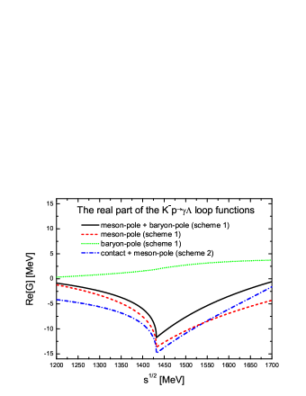
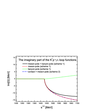
Figure 2: Comparison of the $K^{-}p\rightarrow\gamma\Lambda$ loop functions obtained from different schemes. See text for details.

One can qualitatively understand the results for the partial decay widths of the two poles as follows. The coupling constants for these two poles differ in the relative strength of different channels: For the high-energy pole, the coupling to the $\bar{K}N$ intermediate channel is larger while for the low-energy pole the coupling to the $\pi\Sigma$ channel is larger. Therefore, for the $\gamma\Lambda$ channel, using the coupling constants for the low-energy pole instead of the high-energy pole effectively reduces the contribution of the $K^{-}p$ channel while it enhances the contribution of the $\pi^{+}\Sigma^{-}$ and $\pi^{-}\Sigma^{+}$, but the contributions of the $\pi^{+}\Sigma^{-}$ and $\pi^{-}\Sigma^{+}$ almost cancel each other, and thus, the net effect of using the coupling constants for the low-energy pole instead of the high-energy pole reduces the corresponding decay width.

On the other hand, for the decay mode to the $\gamma\Sigma^{0}$ final state, two things are noteworthy. First, the contribution of the $K^{-}p$ channel is much smaller compared to the contribution of the $K^{-}p$ channel to the decay mode $\gamma\Lambda$. Second, the contributions of $\pi^{+}\Sigma^{-}$ and $\pi^{-}\Sigma^{+}$ add constructively instead of destructively. Therefore, when using the coupling constants for the low-energy pole instead of the high-energy pole, the radiative decay width increases.

At this point, we can conclude that if different experiments actually measure different radiative decay widths for the $\Lambda(1405)$, it can be used as evidence for supporting the two-pole structure of the $\Lambda(1405)$. Instead of the individual radiative decay widths, the ratio between the radiative decay widths to the $\gamma\Lambda$ and $\gamma\Sigma^{0}$ final states might server better this purpose since in one case one has $\Gamma_{\gamma\Lambda}/\Gamma_{\gamma\Sigma^{0}}>1$ and in the other case one has $\Gamma_{\gamma\Lambda}/\Gamma_{\gamma\Sigma^{0}}<1$. This controversy, if confirmed by experiment, can only be explained by assuming that there are actually two poles related to the nominal $\Lambda(1405)$.

At first sight, our calculated decay widths are somehow different from the isobar model fit of H. Burkhardt and J. Lowe Burkhardt:1991ms . However, one should remember that in their fit they used the nominal $\Lambda(1405)$ mass. As we can see in Table 6, when calculated at the nominal $\Lambda(1405)$ mass, with the coupling constants of the high-energy pole, our calculated radiative decay width for the $\gamma\Lambda$ channel is 33.8 keV and for the $\gamma\Sigma^{0}$ is 26.2 keV. On the other hand, if we use the coupling constants for the low-energy pole, the results would be 23.2 keV for the $\gamma\Lambda$ channel and 82.4 keV for the $\gamma\Sigma^{0}$ channel. It is evident that our results with the high-energy pole coupling constants are in good agreement with the results of the isobar model fit: $\Gamma_{\gamma\Lambda}=27\pm 8$ keV and $\Gamma_{\gamma\Sigma^{0}}=23\pm 7$ keV or $10\pm 4$ keV Burkhardt:1991ms , if the calculations are done for the nominal $\Lambda(1405)$ mass. This might indicate that the $K^{-}p$ intermediate channel, and thus the high-energy pole, is dominant in the process analyzed in Ref. Burkhardt:1991ms to deduce the radiative decay widths.

Finally, we would like to stress the importance of the baryon-pole term of the diagram (c) of Fig. 1. If instead of employing gauge invariance and calculating all the three diagrams (a), (b), and (c) of Fig. 1 (we call this scheme 1), we had calculated only diagrams (a) and (b), i.e. only the contact term and the meson-pole term (we call this scheme 2), we would have obtained different results. The corresponding $K^{-}p\rightarrow\gamma\Lambda$ loop functions are plotted in Fig. 2 as a function of the invariant mass of the $MB$ system. The loop functions of scheme 2 are calculated using the cutoff $\Lambda=630$ MeV as in Refs. Oset:1997it ; Lee:1998gt . It is easily seen the baryon-pole term changes the real part of the loop function by $\sim$30%. As a consequence, without this term, the calculated radiative decay width would be larger by almost 40%. It is also interesting to note that the imaginary part of the contact plus meson-pole term of scheme 2 is identical to the imaginary part of the meson-pole term of scheme 1.

4 Exploration of possible reactions

In the previous section, we have shown that the radiative decay widths of the $\Lambda(1405)$ to $\gamma\Lambda$ and $\gamma\Sigma^{0}$ can be very different depending on which of the two poles dominates. Therefore, the good test would be to select different reactions which give different weights to the two poles. Such reactions can provide further evidence for the predicted two-pole structure of the $\Lambda(1405)$. A first evidence for the two-pole structure of the $\Lambda(1405)$ has been provided in Ref. Magas:2005vu . By investigating the invariant mass distribution of the $\pi^{0}\Sigma^{0}$ final state in the $K^{-}p\rightarrow\pi^{0}\pi^{0}\Sigma^{0}$ reaction, it was shown that this reaction gives more weight to the high-energy pole of the $\Lambda(1405)$ in contrast to the reaction $\pi^{-}p\rightarrow K^{0}\pi\Sigma$, where the low-energy pole is believed to be dominant. This $\pi^{-}p\rightarrow K^{0}\pi\Sigma$ reaction has been studied in Ref. Hyodo:2003jw . The authors found that the pure chiral mechanism alone cannot reproduce the experimental invariant mass distributions. However, by explicitly taking into account the contribution of the $N^{*}(1710)$, which gives more weight to the $\pi\Sigma$ channel, and thus more weight to the low-energy pole, they found that the experimental data can be reasonably described. In the following, we study the corresponding electromagnetic reactions $K^{-}p\rightarrow\pi^{0}\gamma\Lambda(\Sigma^{0})$ and $\pi^{-}p\rightarrow K^{0}\gamma\Lambda(\Sigma^{0})$ in more detail.

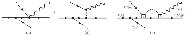
Figure 3: The diagrams contributing to the reaction $K^{-}p\rightarrow\pi^{0}\gamma\Lambda(\Sigma^{0})$.

Figure 4: The strong amplitude $T$.

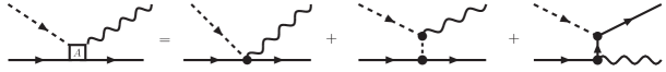
Figure 5: The electromagnetic amplitude $A$.

4.1 The $K^{-}p\rightarrow\pi^{0}\gamma\Lambda(\Sigma^{0})$ reaction

In Ref. Magas:2005vu , it was found that the reaction $K^{-}p\rightarrow\pi^{0}\pi^{0}\Sigma^{0}$ is dominated by the so-called nucleon-pole mechanism. By analogy, the $K^{-}p\rightarrow\pi^{0}\gamma\Lambda(\Sigma^{0})$ reaction should also proceed through the same mechanism, which is explicitly shown in Figs. 3, 4, and 5. The corresponding $t$-matrix reads

$$-it=-iA\vec{\sigma}\cdot\vec{\epsilon}\,\vec{\sigma}\cdot\vec{v}-iB\vec{\epsilon}\cdot\vec{p}_{a}\,\vec{\sigma}\cdot(\vec{p}_{a}-\vec{p}_{2})\,\vec{\sigma}\cdot\vec{v},$$ (19)

where $\vec{v}=\vec{p}_{1}(1+\frac{p_{1}^{0}}{2M_{N}})+\frac{p_{1}^{0}}{M_{N}}\vec{p}_{a}$, $A$ and $B$ are

$$A = \frac{D+F}{2f_{\pi}}\frac{M_{N}}{E_{N}(\vec{p}_{a}+\vec{p}_{1})}\frac{1}{E_{N}-p_{1}^{0}-E_{N}(\vec{p}_{a}+\vec{p}_{1})}$$ (20)

$$\times\Bigg{[}\sum_{j}T_{k^{-}p\rightarrow j}(M_{I})(G^{b}(M_{I})+G^{c}(M_{I}))$$

$$\hskip 34.14322pt\times(-e)Q_{j}\left(\alpha_{j}\frac{D+F}{2f}+\beta_{j}\frac{D-F}{2f}\right)$$

$$\hskip 17.07182pt+(-e)Q_{1}\left(\alpha_{1}\frac{D+F}{2f}+\beta_{1}\frac{D-F}{2f}\right)\Bigg{]},$$

$$B = \frac{D+F}{2f_{\pi}}\frac{M_{N}}{E_{N}(\vec{p}_{a}+\vec{p}_{1})}\frac{1}{E_{N}-p_{1}^{0}-E_{N}(\vec{p}_{a}+\vec{p}_{1})}$$ (21)

$$\times\frac{-2eQ_{1}}{(p_{a}-p_{2})^{2}-m_{a}^{2}}\left[\alpha_{1}\frac{D+F}{2f}+\beta_{1}\frac{D-F}{2f}\right],$$

with $M_{N}$ the nucleon mass, $E_{N}$ the nucleon energy, and $M_{I}^{2}=(p_{2}+p_{3})^{2}$. The last term of Eq. (20) accounts for the first tree level diagram of Fig. 3, while the other part of the $A$ coefficient proportional to $T_{K^{-}p\rightarrow j}$ accounts for the third diagram (loop diagram) of Fig. 3. The term $B$ corresponds to the second tree level diagram of Fig. 3. In Eq. (20), the $T_{k^{-}p\rightarrow j}$, with $j$ referring to the ten coupled channels, are the strong amplitudes of Ref. Oset:2001cn , which is diagrammatically shown in Fig. 4. The loop functions $G^{b}$ and $G^{c}$ are those of Eqs. (12) and (14).

The invariant mass distribution is then calculated by

$$\frac{d\sigma}{dM_{I}} = \frac{1}{4}\frac{M_{N}M_{Y}}{\lambda^{1/2}(s,M_{N}^{2},m_{K}^{2})}\frac{M_{I}}{\sqrt{s}}\frac{1}{(2\pi)^{4}}$$ (22)

$$\times\int^{1}_{-1}d\cos\theta_{1}\int^{E_{\mathrm{max}}}_{E_{\mathrm{min}}}dE_{2}\int^{2\pi}_{0}d\phi_{12}\bar{\sum}\sum|t|^{2}$$

$$\hskip 28.45274pt\times\theta(1-\cos^{2}(\theta_{12}))$$

where $\sqrt{s}$ is the center of mass energy of $K^{-}p$, $\theta_{1}$ is the angle between $\vec{p}_{a}$ and $\vec{p}_{1}$, $\theta_{12}$ is the angle between $\vec{p}_{1}$ and $\vec{p}_{2}$, fixed by kinematics, while $\phi_{12}$ is the azimuthal angle of $\vec{p}_{2}$ with respect to a frame where $\vec{p}_{1}$ is chosen in the $z$ direction. In addition, $E_{\mathrm{min}}=0$, $E_{\mathrm{max}}=\frac{s-(m_{1}+m_{3})^{2}}{2\sqrt{s}}$, and

$$\cos(\theta_{12})=\frac{1}{2|\vec{p}_{1}||\vec{p}_{2}|}\left\{(\sqrt{s}-E_{1}-E_{2})^{2}-m^{2}_{3}-\vec{p}_{1}^{2}-\vec{p}_{2}^{2}\right\},$$ (23)

$$\bar{\sum}\sum|t|^{2} = |v|^{2}\Bigg{\{}\{2|A|^{2}+\left(|\vec{p}_{a}|^{2}-\frac{(\vec{p}_{a}\cdot\vec{p}_{2})^{2}}{|\vec{p}_{2}|^{2}}\right)$$

$$\times\left[(A^{*}B+AB^{*})+|B|^{2}(\vec{p}_{a}-\vec{p}_{2})^{2}\right]\Bigg{\}}.$$

The invariant mass distributions for the reactions $K^{-}p\rightarrow\pi^{0}\gamma\Lambda$ and $K^{-}p\rightarrow\pi^{0}\gamma\Sigma^{0}$ for a kaon of laboratory momentum 687 MeV are shown in Fig. 6. It is seen that both the invariant mass distributions exhibit a peak at $\sim$1420 MeV, and therefore manifesting the high-energy pole of the $\Lambda(1405)$. The invariant mass distribution is also different from a Breit-Wigner shape, particularly that of the $\gamma\Lambda$ channel, which is due to the background terms (the tree-level diagrams in Fig. 3).

It is interesting to recall that in Refs. Oset:1997it ; Oset:2001cn , the two poles, one at 1390 MeV with a width of 132 MeV and the other at 1426 MeV with a width of 32 MeV, are generated through the interaction of the ten coupled channels. The low-energy pole couples more strongly to the $\pi\Sigma$ channel while the high-energy pole couples more strongly to the $\bar{K}N$ channel. It was argued in Ref. Jido:2003cb that reactions favoring different channels would lead to different invariant mass distributions giving more weight to one pole or the other. It should be noted that in Ref. Oset:1997it , the experimental invariant mass distribution was produced by the following formula

$$\frac{d\sigma}{dm_{\alpha}}=C|T_{\pi\Sigma\rightarrow\pi\Sigma}|^{2}P_{\mathrm{CM}},$$ (25)

and thus giving more weight to the low-energy pole and resulting in a peak at $\sim$1400 MeV. However, in the presence of two resonances, the different $T_{ij}$ amplitudes do not peak at the same place, and particularly, $T_{\bar{K}N\rightarrow\pi\Sigma}$ peaks at higher energies than $T_{\pi\Sigma\rightarrow\pi\Sigma}$ Jido:2003cb . In such a case, Eq. (25) should be replaced  Jido:2003cb by

$$\frac{d\sigma}{dm_{\alpha}}=|\sum C_{i}T_{i\rightarrow\pi\Sigma}|^{2}P_{\mathrm{CM}}.$$ (26)

Hence, if the reaction mechanism does not completely forbid a $\bar{K}N$ channel, then the peak should always be shifted towards higher energy. Thus, it is not surprising that the invariant mass distributions of all the three reactions Nacher:1998mi ; Nacher:1999ni ; Magas:2005vu studied previously including the present one exhibit a peak around $\sim$1420 MeV.

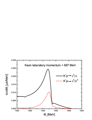
Figure 6: The invariant mass distribution of $K^{-}p\rightarrow\pi^{0}\gamma\Lambda(\gamma\Sigma^{0})$ as a function of the invariant mass of the final $\gamma\Lambda$($\gamma\Sigma^{0}$) system.

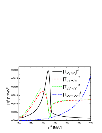
Figure 7: The modulus squared of the strong amplitudes obtained from the model of Ref. Oset:2001cn .

It is worth pointing out an interesting difference between the reactions studied in this work and the other reactions Nacher:1998mi ; Nacher:1999ni ; Magas:2005vu . In the reaction $K^{-}p\rightarrow\pi^{0}\gamma\Lambda(\Sigma^{0})$ and the reaction $\pi^{-}p\rightarrow K^{0}\gamma\Lambda(\Sigma^{0})$, which will be studied below, the $K^{-}p\rightarrow K^{-}p$ channel appears as an intermediate channel. Since the magnitude of the $t$-matrix of this channel is much larger than those of the other channels, and since this channel manifests the high-energy pole (see Fig. 7), one can always expect a peak at $\sim 1420$ MeV in the invariant mass distribution of the final states unless some reaction mechanisms largely suppress this channel. On the other hand, in the $\pi\Sigma$ final states studied in Refs. Nacher:1998mi ; Nacher:1999ni ; Magas:2005vu , the $T_{\bar{K}N\rightarrow\bar{K}N}$ does not contribute and because the $\bar{K}N\rightarrow\pi\Sigma$ and $\pi\Sigma\rightarrow\pi\Sigma$ amplitudes have similar strength (in fact the modulus of the $K^{-}p\rightarrow\pi\Sigma$ amplitude is still approximately two times larger than that of the $\pi\Sigma\rightarrow\pi\Sigma$ amplitude at their respective peak positions), the invariant mass distributions will be a superposition of the two peaks, and, depending on the reaction mechanism, the final distribution will peak at one or another energy. This situation is somewhat similar to the two-pole structure of the $K_{1}(1270)$ Geng:2006yb . There, it was found that due to the dominance of the $\rho K\rightarrow\rho K$ amplitude over the other amplitudes leading to the $\rho K$ final states, a prominent peak at $\sim 1280\,\mbox{MeV}$ would be preferred in the invariant mass distribution of the $K\pi\pi$ system leading to $\rho K$ final states.

Figure 8: The diagrams contributing to the reaction $\pi^{-}p\rightarrow K^{0}\gamma\Lambda(\Sigma^{0})$.

4.2 The $\pi^{-}p\rightarrow K^{0}\gamma\Lambda(\Sigma^{0})$ reaction

In Ref. Hyodo:2003jw , it was shown that the reaction $\pi^{-}p\rightarrow K^{0}\pi\Sigma$ can be reasonably described in terms of $t$-channel and $s$-channel resonance exchanges. The corresponding electromagnetic reaction $\pi^{-}p\rightarrow K^{0}\gamma\Lambda(\Sigma^{0})$, in principle, should also proceed through similar mechanisms. Nevertheless, since we only want to make an exploratory study of this reaction, we neglect the mechanisms of $t$-channel meson exchange (and associated contact $MMBBB$ terms), referred to as chiral terms in Ref. Hyodo:2003jw , and concentrate on the $s$-wave $N^{*}(1710)$ resonance contribution, which was found to be largely dominant in Ref. Hyodo:2003jw .

The $t$-matrix element corresponding to the resonance mechanism shown in Fig. 8 reads

$$-it = (-it_{\pi^{-}p\rightarrow N^{*}})\frac{i}{\sqrt{s}-M_{\mathrm{R}}+i\frac{\Gamma}{2}}$$ (27)

$$\hskip 28.45274pt\times\sum_{i}(-it_{N^{*}\rightarrow K^{0}i})(-it_{i\rightarrow\gamma\Lambda(\Sigma^{0})})$$

with

$$-it_{\pi^{-}p\rightarrow N^{*}}=\frac{A}{f_{\pi}}\vec{\sigma}\cdot\vec{p}_{a},$$ (28)

$$-it_{N^{*}\rightarrow K^{0}i}=i\frac{\tilde{B}}{f^{2}}C_{i}(\omega_{i}-\omega_{K^{0}}),$$ (29)

$$-it_{i\rightarrow\gamma\Lambda(\Sigma^{0})} = \sum_{j}\left(G_{i}(M_{I})T_{i\rightarrow j}(M_{I})+\delta_{ij}\right)(G^{b}_{j}+G^{c}_{j})\vec{\sigma}\cdot\vec{\epsilon}$$ (30)

$$\times\left[-ieQ_{j}\left(\alpha_{j}\frac{D+F}{2f}+\beta_{j}\frac{D-F}{2f}\right)\right],$$

where $i$, $j$ can be any of the ten coupled channels. The couplings constants $C_{i}$ can be found in Table II of Ref. Hyodo:2003jw . The loop function $G_{i}$ is that of one meson and one baryon, which is calculated in the dimensional regularization scheme and with the same subtraction constants as in Ref. Oset:2001cn . The meson energies $\omega_{i}$ and $\omega_{K^{0}}$ are calculated by

$$\omega_{K^{0}}=\frac{s+m^{2}_{K}-M^{2}_{I}}{2\sqrt{s}},$$ (31)

$$\omega_{i}=\frac{M^{2}_{I}+m^{2}_{i}-M^{2}_{i}}{2M_{I}},$$ (32)

with $\sqrt{s}$ the invariant mass of $\pi^{-}p$, $m_{i}$ and $M_{i}$ the meson and baryon masses of channel $i$, and $M_{I}$ the $\gamma\Lambda(\Sigma^{0})$ invariant mass.

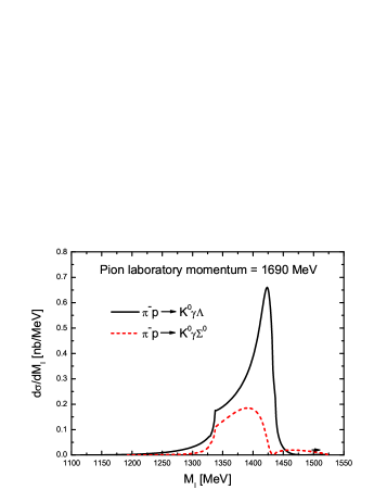
Figure 9: The invariant mass distribution of $\pi^{-}p\rightarrow K^{0}\gamma\Lambda(\gamma\Sigma^{0})$ as a function of the invariant mass of the final $\gamma\Lambda$($\gamma\Sigma^{0}$) system.

In our calculation, the parameter set II of Ref. Hyodo:2003jw is used, i.e. $M_{R}=1740$ MeV, $|A|=0.1344$, $|\tilde{B}|=0.842$, $\Gamma(\sqrt{s}=2020\mbox{ MeV})=776$ MeV. The invariant mass distributions are calculated by

$$\frac{d\sigma}{dM_{I}}=\frac{M_{N}M_{Y}}{\lambda^{1/2}(s,M^{2}_{N},m^{2}_{\pi})}\frac{1}{(2\pi)^{3}}\frac{1}{\sqrt{s}}p_{1}\tilde{p}_{2}\bar{\sum}\sum|t|^{2}$$ (33)

with

$$p_{1}=\frac{\lambda^{1/2}(s,M_{I}^{2},m_{1}^{2})}{2\sqrt{s}},\quad\tilde{p}_{2}=\frac{\lambda^{1/2}(M_{I}^{2},m_{2}^{2},m_{3}^{2})}{2M_{I}},$$ (34)

and are shown in Fig. 9 for a pion of laboratory momentum 1690 MeV. At first sight, two things are surprising. First, the $\pi^{-}p\rightarrow K^{0}\gamma\Lambda$ reaction still exhibits a peak around $\sim$1420 MeV. Second, the magnitude of the $\pi^{-}p\rightarrow K^{0}\gamma\Lambda$ is still larger than that of $\pi^{-}p\rightarrow K^{0}\gamma\Sigma^{0}$. This is due to the following reasons: As we have noticed in the previous section, the $\pi^{+}\Sigma^{-}\rightarrow\gamma\Lambda$ term and the $\pi^{-}\Sigma^{+}\rightarrow\gamma\Lambda$ term nearly cancel each other. Therefore, it is natural that the $\pi^{-}p\rightarrow K^{0}\gamma\Lambda$ reaction still manifests the high-energy pole of the $\Lambda(1405)$ since in this reaction the $K^{-}p\rightarrow\gamma\Lambda$ intermediate channel contributes most. While in the $\pi^{-}p\rightarrow K^{0}\gamma\Sigma^{0}$ reaction, the contribution of $K^{-}p\rightarrow\gamma\Sigma^{0}$ itself is small and is further suppressed by the $\omega_{K^{-}}-\omega_{K^{0}}$ factor of Eq. (29). On the other hand, the $\pi^{+}\Sigma^{-}\rightarrow\gamma\Sigma^{0}$ and $\pi^{-}\Sigma^{+}\rightarrow\gamma\Sigma^{0}$ terms add constructively and both give more weight to the low-energy pole of the $\Lambda(1405)$. Therefore, the net result is a broad peak around $\sim$1390 MeV, in agreement with the finding of Ref. Hyodo:2003jw . The larger magnitude of $\pi^{-}p\rightarrow K^{0}\gamma\Lambda$ is due to the fact that the strong amplitude $K^{-}p\rightarrow K^{-}p$ is much larger than the other $i\rightarrow j$ amplitudes, as we have discussed previously.

5 Summary and conclusions

Using the unitary extension of the chiral perturbation theory U$\chi$PT, we have calculated the radiative decay widths of the $\Lambda(1405)$. Since there are two poles in the U$\chi$PT models corresponding to the nominal $\Lambda(1405)$, our calculations, using the model of Refs. Oset:1997it ; Oset:2001cn , result in two different radiative decay widths. For the high-energy pole, our calculated widths, $\Gamma_{\gamma\Lambda}$=64.8 keV and $\Gamma_{\gamma\Sigma^{0}}$=33.5 keV, are in qualitative agreement with the predictions of the isobar model fit, in particular, when evaluated at the nominal $\Lambda(1405)$ mass where the agreement is very good, but they are in sharp contrast with those of the quark models and the bag models. The disagreement with the quark model predictions adds to the list of other magnitudes that the quark models also fail to reproduce. For instance, the $\Lambda(1405)$ and the $\Lambda(1520)$ are degenerate in the model of Ref. Isgur:1978xj .

We also evaluated the radiative decay width for the low-energy pole, and we obtain a totally different result with $\Gamma_{\gamma\Lambda}=16.1$ keV and $\Gamma_{\gamma\Sigma^{0}}=73.5$ keV. These are completely different from all the existing model predictions. All the other theoretical models predict a larger $\gamma\Lambda$ decay width while a smaller $\gamma\Sigma^{0}$ decay width except the algebraic model Bijker:2000gq .

To find a possible reaction which might give different weights to the two poles of the $\Lambda(1405)$, we have studied the reactions $K^{-}p\rightarrow\pi^{0}\gamma\Lambda(\Sigma^{0})$ and $\pi^{-}p\rightarrow K^{0}\gamma\Lambda(\Sigma^{0})$. These two reactions share a lot of similarities with the corresponding hadronic reactions, $K^{-}p\rightarrow\pi^{0}\pi^{0}\Sigma^{0}$ and $\pi^{-}p\rightarrow K^{0}\pi\Sigma$, which have been previously studied in Refs. Magas:2005vu ; Hyodo:2003jw and found to yield reasonable agreement with the data. Our studies show that both these reactions yield a larger $\gamma\Lambda$ cross section and a smaller $\gamma\Sigma^{0}$ cross section. This reflects a non-trivial feature of the U$\chi$PT model: the magnitude of the $K^{-}p\rightarrow K^{-}p$ amplitude is much larger than that of the other amplitudes. On the other hand, there are subtle differences between the two reactions studied, $K^{-}p\rightarrow\pi^{0}\gamma\Lambda(\Sigma^{0})$ and $\pi^{-}p\rightarrow K^{0}\gamma\Lambda(\Sigma^{0})$. While the first reaction gives more weight to the high-energy pole in both channels, the second reaction gives more weight to the high-energy pole in the $\gamma\Lambda$ channel and to the low-energy pole in the $\gamma\Sigma^{0}$ channel. This is reflected by exhibiting a narrower peak at $\sim 1420$ MeV in the former channel and a broader peak at $\sim 1390$ MeV in the latter channel. The total cross sections for the $K^{-}p$ reaction at $p_{K}(\mbox{lab})=687$ MeV are 1.78 $\mu b$ ($\gamma\Lambda)$ and 0.41 $\mu b$ ($\gamma\Sigma^{0}$), which are integrated [see Eq. (22)] with the lower limit $M_{I}=1300\,$MeV to avoid infrared divergence. The cross sections for the $\pi^{-}p$ reaction at $p_{\pi}(\mbox{lab})=1690$ MeV turn out to be $3.90\times 10^{-2}$ $\mu b$ ($\gamma\Lambda$) and $1.58\times 10^{-2}$ $\mu b$ ($\gamma\Sigma^{0}$).

Therefore, an experimental measurement of the radiative decay widths of the $\Lambda(1405)$ in the related reactions, such as $K^{-}p\rightarrow\pi^{0}\gamma\Lambda(\Sigma^{0})$ and $\pi^{-}p\rightarrow K^{0}\gamma\Lambda(\Sigma^{0})$, not only would lend further support to the predicted two-pole structure of the $\Lambda(1405)$ but also to the underlying chiral unitary approach, which so far has provided a systematic and consistent description of the $\Lambda(1405)$ and low-energy reactions involving it.

6 Acknowledgments

L. S. Geng acknowledges useful communications with Dr. T. Hyodo and financial support from the Ministerio de Educacion y Ciencia in the Program of estancias de doctores y tecnologos extranjeros. This work is partly supported by DGICYT contract number Fis2006-03438 and the Generalitat Valenciana. This research is part of the EU Integrated Infrastructure Initiative Hadron Physics Project under contract number RII3-CT-2004-506078.

Appendix A Basic diagrams

1. The lowest-order interaction Lagrangian related to the $MBB$ term is

   $$\mathcal{L}=\frac{D+F}{2}\langle\bar{B}\gamma^{\mu}\gamma_{5}u_{\mu}B\rangle+\frac{D-F}{2}\langle\bar{B}\gamma^{\mu}\gamma_{5}Bu_{\mu}\rangle,$$ (35)

   where $u_{\mu}=-\frac{\sqrt{2}}{f}\partial_{\mu}\Phi$. This leads to the following Feymann rule (with incoming meson momentum $k_{\mu}$):

   $$-it=i\mathcal{L}=-\gamma^{\mu}\gamma_{5}k_{\mu}\left(\alpha\frac{D+F}{2f}+\beta\frac{D-F}{2f}\right).$$ (36)

   With the non-relativistic reduction $\gamma^{\mu}\gamma_{5}k_{\mu}\rightarrow-\vec{\sigma}\vec{k}$, the $t$-matrix reads:

   $$-it=i\mathcal{L}=\vec{\sigma}\vec{k}\left(\alpha\frac{D+F}{2f}+\beta\frac{D-F}{2f}\right).$$ (37)

2. The contact (Kroll-Ruderman) term can be obtained by applying the minimal substitution in Eq. (35), i.e. $\partial_{\mu}\Phi\rightarrow(\partial_{\mu}+ieA_{\mu})\Phi$, which leads to the following Feynman rule:

   $$(-it)=i\mathcal{L}=-eQ\vec{\sigma}\vec{\epsilon}\left(\alpha\frac{D+F}{2f}+\beta\frac{D-F}{2f}\right),$$ (38)

   where $Q$ is the charge of the meson.

References

- (1) N. Isgur and G. Karl, Phys. Rev. D 18, 4187 (1978).
- (2) R. H. Dalitz and S. F. Tuan, Annals Phys. 10, 307 (1960).
- (3) N. Kaiser, T. Waas and W. Weise, Nucl. Phys. A 612, 297 (1997).
- (4) E. Oset and A. Ramos, Nucl. Phys. A 635, 99 (1998).
- (5) E. Oset, A. Ramos and C. Bennhold, Phys. Lett. B 527, 99 (2002) [Erratum-ibid. B 530, 260 (2002)].
- (6) J. A. Oller and U. G. Meissner, Phys. Lett. B 500, 263 (2001).
- (7) D. Jido, J. A. Oller, E. Oset, A. Ramos and U. G. Meissner, Nucl. Phys. A 725, 181 (2003).
- (8) C. Garcia-Recio, J. Nieves, E. Ruiz Arriola and M. J. Vicente Vacas, Phys. Rev. D 67, 076009 (2003).
- (9) C. Garcia-Recio, M. F. M. Lutz and J. Nieves, Phys. Lett. B 582, 49 (2004).
- (10) T. Hyodo, S. I. Nam, D. Jido and A. Hosaka, Phys. Rev. C 68, 018201 (2003).
- (11) B. Borasoy, R. Nissler and W. Weise, Eur. Phys. J. A 25, 79 (2005).
- (12) J. A. Oller, J. Prades and M. Verbeni, Phys. Rev. Lett. 95, 172502 (2005).
- (13) J. A. Oller, Eur. Phys. J. A 28, 63 (2006).
- (14) B. Borasoy, U. G. Meissner and R. Nissler, Phys. Rev. C 74, 055201 (2006).
- (15) J. C. Nacher, E. Oset, H. Toki and A. Ramos, Phys. Lett. B 455, 55 (1999).
- (16) J. C. Nacher, E. Oset, H. Toki and A. Ramos, Phys. Lett. B 461, 299 (1999).
- (17) T. Hyodo, A. Hosaka, E. Oset, A. Ramos and M. J. Vicente Vacas, Phys. Rev. C 68, 065203 (2003).
- (18) S. Prakhov et al. [Crystall Ball Collaboration], Phys. Rev. C 70, 034605 (2004).
- (19) V. K. Magas, E. Oset and A. Ramos, Phys. Rev. Lett. 95, 052301 (2005).
- (20) S. Taylor et al. [CLAS Collaboration], Phys. Rev. C 71, 054609 (2005) [Erratum-ibid. C 72, 039902 (2005)].
- (21) F. Myhrer, Phys. Rev. C 74, 065202 (2006).
- (22) D. A. Whitehouse, Phys. Rev. Lett. 63, 1352 (1989).
- (23) H. Burkhardt and J. Lowe, Phys. Rev. C 44, 607 (1991).
- (24) T. S. H. Lee, J. A. Oller, E. Oset and A. Ramos, Nucl. Phys. A 643, 402 (1998).
- (25) B. Borasoy, P. C. Bruns, U. G. Meissner and R. Nissler, Phys. Rev. C 72, 065201 (2005).
- (26) M. Döring, E. Oset and S. Sarkar, Phys. Rev. C 74, 065204 (2006).
- (27) M. Doring, E. Oset and D. Strottman, Phys. Rev. C 73, 045209 (2006).
- (28) D. A. Whitehouse, Ph.D. thesis, Boston University, 1988.
- (29) M. Döring, Nucl. Phys. A 786, 164 (2007).
- (30) F. E. Close, N. Isgur and S. Kumano, Nucl. Phys. B 389, 513 (1993).
- (31) J. A. Oller, Phys. Lett. B 426, 7 (1998).
- (32) E. Marco, S. Hirenzaki, E. Oset and H. Toki, Phys. Lett. B 470, 20 (1999).
- (33) L. Roca, A. Hosaka and E. Oset, arXiv:hep-ph/0611075.
- (34) M. E. Peskin and D. V. Schroeder, An Introduction To Quantum Field Theory, Perseus Books, Massachusetts, 1995.
- (35) L. Yu, X. L. Chen, W. Z. Deng and S. L. Zhu, Phys. Rev. D 73, 114001 (2006).
- (36) T. Van Cauteren, J. Ryckebusch, B. Metsch and H. R. Petry, Eur. Phys. J. A 26, 339 (2005).
- (37) J. W. Darewych, M. Horbatsch and R. Koniuk, Phys. Rev. D 28, 1125 (1983).
- (38) E. Kaxiras, E. J. Moniz and M. Soyeur, Phys. Rev. D 32, 695 (1985).
- (39) M. Warns, W. Pfeil and H. Rollnik, Phys. Lett. B 258, 431 (1991).
- (40) Y. Umino and F. Myhrer, Nucl. Phys. A 554, 593 (1993).
- (41) C. L. Schat, N. N. Scoccola and C. Gobbi, Nucl. Phys. A 585, 627 (1995).
- (42) R. Bijker, F. Iachello and A. Leviatan, Annals Phys. 284, 89 (2000).
- (43) L. S. Geng, E. Oset, L. Roca and J. A. Oller, Phys. Rev. D 75, 014017 (2007).