Exclusive processes $e^{+}e^{-}\to VP$ in $k_{T}$ factorization

Abstract

The exclusive processes $e^{+}e^{-}\to VP$, in the region of which the final state meson momentum is much larger than the hadronic scale $\Lambda_{QCD}$, are studied in the framework of PQCD approach based on the $k_{T}$ factorization. Including the transverse momentum distribution in the light cone wave functions, our results are consistent with the experimental measurements. According to our results, many processes have large enough cross sections to be detected at $\sqrt{s}=10.58$ GeV. The $s$ dependence of the cross section has been directly studied and our result indicates that the $1/s^{3}$ scaling is more favored than $1/s^{4}$. We also find that the gluonic contribution for the processes involving $\eta^{(^{\prime})}$ is tiny.

I Introduction

In exclusive or inclusive processes with large momentum transfers, the production rates and many other phenomena, such as the dimensional rule, the helicity structure, can be successfully explained by the perturbative QCD analysis pQCDBL ; pQCDER . The essential ingredient is the factorization theorem which insures that a physical amplitude can be represented as a convolution of a hard scattering kernel and hadron distribution amplitudes. The former can be calculated using the perturbation theory while the latter, although non-perturbative in nature, are universal. The light cone distribution amplitudes which describe the longitudinal momentum distribution of partons in hadron, can be determined by the experiments of various channels. In $e^{+}e^{-}\to\gamma^{*}\to VP$ at high energies (V denotes a light vector meson and P denotes a light pseudoscalar meson), the energy of the light meson is much larger than its mass and the hadronic scale $\Lambda_{QCD}$. One important feature of this process is that the meson moves nearly on the light cone. The energetic light meson is composed of two valence quarks which are both energetic and collinear. The gluon which generates the quark pair is very hard and this leads to the application of perturbative QCD into this process. However, the application of the perturbative QCD approach to this simple process is complicated by the end point problem. If collinear factorization is applied, the hard kernel contains the inverse term of momentum fraction which makes the integration divergent at the end point. This divergence arises from the overlap of the soft and collinear momentum region . A modified perturbative QCD approach based on $k_{T}$ factorization, which keeps the intrinsic transverse momentum of partons in the meson, is proposed and successfully applied to many processes PQCDLS ; PQCDBdecay . In this approach, the Sudakov effect is taken into account and the applicability of perturbative QCD can be extended down to a few GeV scale. It is claimed that the perturbative calculations could be consistent at scale about $Q\sim 20\Lambda_{QCD}$ in this framework. This approach is also called PQCD approach for simplicity.

The exclusive two-meson productions in $e^{+}e^{-}$ annihilation provide an opportunity to investigate the behaviors of various meson form factors. The dependence of the form factor on the energy scale can shed light on the internal strong interaction information. It can also give information on the wave function of the hadrons in terms of its partonic constituents. In the standard model, the exclusive production of hadron pairs at $e^{+}e^{-}$ colliders can proceed through a virtual photon or a $Z^{0}$ boson. At energies well below the mass of $Z^{0}$, the production proceeds predominantly via the annihilation of $e^{+}e^{-}$ into a virtual photon. Due to the invariance of charge conjugation in electromagnetic and strong interactions, the final state should have the same charge conjugation quantum number with a photon, i.e., these processes can only produce final states with charge conjugation quantum number $C=-1$. $e^{+}e^{-}\to VP$ can proceed via the following form factor:

$$\langle V(\epsilon,p_{1})P(p_{2})|j_{\mu}^{em}|0\rangle=F_{VP}(s)\epsilon_{\mu\nu\alpha\beta}\epsilon^{\nu}p_{1}^{\alpha}p_{2}^{\beta},$$ (1)

where $p_{1}(p_{2})$ is the momentum of the vector (pseudoscalar) meson and $\epsilon$ is the polarization vector of the vector meson. Here $j_{\mu}^{em}$ is defined as $j_{\mu}^{em}=\bar{q}\gamma_{\mu}q$. Eq. (1) indicates that the vector meson is transversely polarized. On the experimental side, the productions of $VP$ have been extensively studied: BES and CLEO-c have reported the continuum productions ExpVP1 ; ExpVP2 ; ExpVP3 . Recently, BaBar Collaboration observed the exclusive reaction $e^{+}e^{-}\to\phi\eta$ at $\sqrt{s}=10.58$GeV and measured the cross section phietaBaBar . Since $k_{T}$ factorization can give a reliable prediction in other similar processes, in this paper, we will perform a study on $e^{+}e^{-}\to\gamma^{*}\to VP$ in this framework and make a comparison with the data.

Another interesting reason for investigating the $e^{+}e^{-}$ annihilation is the similarity with the annihilation corrections in $B$ decays, shown in Fig. 1. In charmless two body $B$ decays, the annihilation diagrams are power suppressed relative to the emission contribution. But it is found that in $B\to\pi K$, $\pi\pi$ decays, the factorizable annihilation diagrams could be important due to the chiral enhancement factor for operator $O_{6}$ PQCDBdecay . This enhancement of factorizable diagrams can provide large strong phases and give large $CP$ asymmetries, which indicates the annihilation diagrams are of great importance. Comparing the two diagrams in Fig. 1, we can see that the $e^{+}e^{-}$ annihilations have similar topologies with the factorizable annihilation diagrams in $B$ decays. They may provide an ideal laboratory to isolate the power correction effect and to find out whether contributions of annihilations from end-point are important or not for meson productions VPandB .

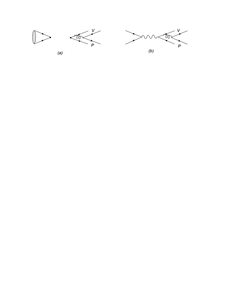
Figure 1: The annihilation diagrams in $B$ decays and $e^{+}e^{-}$ annihilation. In the left diagram, $B$ meson is annihilated through the four-quark operator. In the right diagram, electron and positron annihilate into a virtual photon. These two diagrams have similar topologies.

The remainder of this paper is organized as follows. In Section II, we present the expression for the cross sections for $e^{+}e^{-}\to VP$ in the $k_{T}$ factorization: the first part of this section is devoted to the discussion on the decay constants and the distribution amplitudes of mesons, and the second part contributes to a brief introduction to PQCD approach and factorization formulae for form factors. The numerical results and discussions are presented in Section III. The last section is our summary.

II Calculation in $k_{T}$ factorization

II.1 Decay constants and Wave functions

The decay constants for a pseudoscalar meson and a vector meson are defined by:

$$\langle P(P)|\bar{q}_{2}\gamma_{\mu}\gamma_{5}q_{1}|0\rangle=-if_{P}P_{\mu},\;\;\langle V(P,\epsilon)|\bar{q}_{2}\gamma_{\mu}q_{1}|0\rangle=f_{V}m_{V}\epsilon_{\mu},\;\;\langle V(P,\epsilon)|\bar{q}_{2}\sigma_{\mu\nu}q_{1}|0\rangle=-if_{V}^{T}(\epsilon_{\mu}P_{\nu}-\epsilon_{\nu}P_{\mu}),$$ (2)

The pseudoscalar decay constants taken from the Particle Data Group PDG are shown in Table 1. The charged vector meson longitudinal decay constants are extracted from the data on $\tau^{-}\to(\rho^{-},K^{*-})\nu_{\tau}$, while the neutral vector meson longitudinal decay constants are determined from the data on the electromagnetic annihilation processes $V^{0}\to e^{+}e^{-}$ PDG . The transverse decay constants are taken from the QCD sum rules LCSRBZ ; adoptedvectorwf , which are also collected in Table 1.

Table 1: Input values of the decay constants of the pseudoscalar and vector mesons (in MeV) PDG ; LCSRBZ ; adoptedvectorwf

$f_{\pi}$	$f_{K}$	$f_{\rho}$	$f_{\rho}^{T}$	$f_{\omega}$	$f_{\omega}^{T}$	$f_{K^{*}}$	$f_{K^{*}}^{T}$	$f_{\phi}$	$f_{\phi}^{T}$
131	160	$209$	$165\pm 9$	$195$	$145\pm 10$	$217$	$185\pm 10$	$231$	$200\pm 10$

The light-cone distribution amplitudes are defined by the matrix elements of the non-local operators at the light-like separations $z_{\mu}$ with $z^{2}=0$, and sandwiched between the vacuum and the meson state. The two-particle light-cone distribution amplitudes of an outgoing pseudoscalar meson $P$, up to twist-3 accuracy, are defined by PseudoscalarWV :

$$\langle P(P)|{\bar{q}}_{2\beta}(z)q_{1\alpha}(0)|0\rangle = -\frac{i}{\sqrt{6}}\int_{0}^{1}dxe^{ixP\cdot z}\left[\gamma_{5}\not\!P\phi^{A}(x)+m_{0}\gamma_{5}\phi^{P}(x)-m_{0}\sigma^{\mu\nu}\gamma_{5}P_{\mu}z_{\nu}\frac{\phi^{\sigma}(x)}{6}\right]_{\alpha\beta}$$ (3)

$$= -\frac{i}{\sqrt{6}}\int_{0}^{1}dxe^{ixP\cdot z}\left[\gamma_{5}\not\!P\phi^{A}(x)+\gamma_{5}m_{0}\phi^{P}(x)+m_{0}\gamma_{5}(\not\!n\not\!v-1)\phi^{T}(x)\right]_{\alpha\beta}\;,$$

where $n,v$ are two light-cone vectors. The pseudoscalar meson is moving on the direction of $n$, with $v$ the opposite direction. $m_{0}=\frac{M_{P}^{2}}{m_{q_{1}}+m_{q_{2}}}$ is the chiral enhancement parameter. $x$ is the momentum fraction carried by the positive quark $q_{2}$. We have performed the integration by parts for the third term and $\phi^{T}(x)=\frac{1}{6}{d\over dx}\phi^{\sigma}(x)$. The explicit form of distribution amplitudes for pseudoscalar mesons have been studied in QCD sum rule approach and other methods PseudoscalarUpdate ; NewPWV . In principle, they are factorization scale dependent. Here we use the following form for leading twist distribution amplitudes

$$\phi_{\pi}^{A}(x) = \frac{3f_{\pi}}{\sqrt{6}}x(1-x)[1+a_{2}^{\pi}C_{2}^{3/2}(t)],$$ (4)

$$\phi_{K}^{A}(x) = \frac{6f_{K}}{2\sqrt{6}}x(1-x)[1+a_{1}^{K}C_{1}^{3/2}(t)+a_{2}^{K}C_{2}^{3/2}(t)],$$ (5)

where $t=2x-1$ and Gegenbauer polynomials defined as:

$$C^{3/2}_{1}(t)=3t,C_{2}^{3/2}(t)=\frac{3}{2}(5t^{2}-1).$$ (6)

The Gegenbauer moments at $\mu=1$ GeV are determined as

$$a_{2}^{\pi,K}=0.25\pm 0.15,\;\;\;a_{1}^{K}=0.06\pm 0.03.$$ (7)

Since the momentum transfer at $\sqrt{s}=10.58$ GeV is large enough, the use of asymptotic forms for twist-3 distribution amplitudes is acceptable. Besides, we also use these forms at $\sqrt{s}=3.67$ GeV for simplicity. The asymptotic forms of twist-3 distribution amplitudes are given as:

$$\phi_{\pi(K)}^{P}(x) = \frac{f_{\pi(K)}}{2\sqrt{6}},\;\;\;\phi_{\pi(K)}^{T}(x)=\frac{f_{\pi(K)}}{2\sqrt{6}}(1-2x).$$ (8)

As for the mixing of $\eta$ and $\eta^{\prime}$, we use the quark flavor basis proposed by Feldmann and Kroll FKmixing , i.e. these two mesons are made of $\bar{n}n=(\bar{u}u+\bar{d}d)/\sqrt{2}$ and $\bar{s}s$:

$$\left(\begin{array}[]{c}|\eta\rangle\\ |\eta^{\prime}\rangle\end{array}\right)=U(\theta)\left(\begin{array}[]{c}|\eta_{n}\rangle\\ |\eta_{s}\rangle\end{array}\right),$$ (9)

with the mixing matrix,

$$U(\theta)=\left(\begin{array}[]{cc}\cos\theta&~{}-\sin\theta\\ \sin\theta&\phantom{~{}-}\cos\theta\end{array}\right)\;,$$ (10)

where the mixing angle $\theta=39.3^{\circ}\pm 1.0^{\circ}$. In principle, this mixing mechanism is equivalent to the singlet and octet formalism, which is shown in GluonicCKL . But the advantage is transparent, since only two decay constants are needed:

$$\langle 0|\bar{n}\gamma^{\mu}\gamma_{5}n|\eta_{n}(P)\rangle = \frac{i}{\sqrt{2}}\,f_{n}\,P^{\mu}\;,$$

$$\langle 0|\bar{s}\gamma^{\mu}\gamma_{5}s|\eta_{s}(P)\rangle = if_{s}\,P^{\mu}\;.$$ (11)

We assume that the wave function of $\bar{n}n$ and $\bar{s}s$ is the same as the pion’s wave function, except for the different decay constants and the chiral scale parameters:

$$f_{n}=(1.07\pm 0.02)f_{\pi},\ \ \ f_{s}=(1.34\pm 0.06)f_{\pi}.$$ (12)

The chiral enhancement factors are chosen as

$$m_{0}^{\bar{n}n}=\frac{1}{2m_{n}}[m^{2}_{\eta}\cos^{2}\theta+m_{\eta^{\prime}}^{2}\sin^{2}\theta-\frac{\sqrt{2}f_{s}}{f_{n}}(m_{\eta^{\prime}}^{2}-m_{\eta}^{2})\cos\theta\sin\theta],$$ (13)

$$m_{0}^{\bar{s}s}=\frac{1}{2m_{s}}[m^{2}_{\eta^{\prime}}\cos^{2}\theta+m_{\eta}^{2}\sin^{2}\theta-\frac{f_{n}}{\sqrt{2}f_{s}}(m_{\eta^{\prime}}^{2}-m_{\eta}^{2})\cos\theta\sin\theta],$$ (14)

with $m_{n}=5.6$ MeV and $m_{s}=137$ MeV at $\mu=1$ GeV NewPWV .

In this work, we also investigate the gluonic contribution for iso-singlet pseudoscalar meson $\eta$ and $\eta^{\prime}$. This contribution has been attempted in GluonicCKL with negligible effect in $B\to\eta$ form factor and a few percents to $B\to\eta^{\prime}$. The leading-twist gluonic distribution amplitudes of the $\eta_{n}$ and $\eta_{s}$ mesons are defined as leadingtwistofeta :

$$\langle\eta_{n}(P)|A_{[\mu}^{a}(z)A_{\nu]}^{b}(0)|0\rangle = \frac{\sqrt{2}f_{n}}{\sqrt{3}}\frac{C_{F}}{4\sqrt{3}}\frac{\delta^{ab}}{N_{c}^{2}-1}\epsilon_{\mu\nu\rho\sigma}\,\frac{n_{-}^{\rho}P^{\sigma}\,}{n_{-}\cdot P}\int_{0}^{1}dxe^{ixP\cdot z}\frac{\phi_{n}^{G}(x)}{x(1-x)}\;,$$

$$\langle\eta_{s}(P)|A_{[\mu}^{a}(z)A_{\nu]}^{b}(0)|0\rangle = \frac{f_{s}}{\sqrt{3}}\frac{C_{F}}{4\sqrt{3}}\frac{\delta^{ab}}{N_{c}^{2}-1}\epsilon_{\mu\nu\rho\sigma}\,\frac{n_{-}^{\rho}P^{\sigma}\,}{n_{-}\cdot P}\int_{0}^{1}dxe^{ixP\cdot z}\frac{\phi_{s}^{G}(x)}{x(1-x)}\;,$$ (15)

where $A_{[\mu}^{a}(z)A_{\nu]}^{b}(w)\equiv[A_{\mu}^{a}(z)A_{\nu}^{b}(w)-A_{\nu}^{a}(z)A_{\mu}^{b}(w)]/2$ and the function Gegenbauerofeta ,

$$\phi_{n(s)}^{G}(x)=x^{2}(1-x)^{2}B_{2}^{n(s)}C_{1}^{5/2}(2x-1)\;,\;\;\;\;C_{1}^{5/2}(t)=5t\;.$$ (16)

The gluon labeled by the subscript $\mu$ carries the momentum fractions $x$ based on the above definition. The two Gegenbauer coefficients $B_{2}^{n}$ and $B_{2}^{s}$ could not be the same in principle. However, it is acceptable to assume $B_{2}^{n}=B_{2}^{s}\equiv B_{2}$, since there are large uncertainties in their values. Here the range of $B_{2}$ has been extracted as $B_{2}=4.6\pm 2.5$ leadingtwistofeta .

Following the similar procedures as for the pseudoscalar mesons, we can derive the vector meson distribution amplitudes for the transverse polarization up to twist-3 rho :

$$\langle V(P,\epsilon_{T})|\bar{q}_{2\beta}(z)q_{1\alpha}(0)|0\rangle = \frac{1}{\sqrt{6}}\int_{0}^{1}dxe^{ixP\cdot z}\left[M_{V}\not\!\epsilon_{T}\phi_{V}^{v}(x)+\not\!\epsilon_{T}\not\!P\phi_{V}^{T}(x)\right.$$ (17)

$$\left.+M_{V}i\epsilon_{\mu\nu\rho\sigma}\gamma_{5}\gamma^{\mu}\epsilon_{T}^{\nu}n^{\rho}v^{\sigma}\phi_{V}^{p}(x)\right]_{\alpha\beta},\;$$

where we have adopted the convention $\epsilon^{0123}=1$ for the Levi-Civita tensor $\epsilon^{\mu\nu\alpha\beta}$.

The twist-2 distribution amplitudes for transversely polarized vector can be expanded as:

$$\phi^{T}_{\rho}(x) = \frac{3f^{T}_{\rho}}{\sqrt{6}}x(1-x)\left[1+a_{2\rho}^{\perp}C_{2}^{3/2}(t)\right]\;,$$ (18)

$$\phi^{T}_{\omega}(x) = \frac{3f^{T}_{\omega}}{\sqrt{6}}x(1-x)\left[1+a_{2\omega}^{\perp}C_{2}^{3/2}(t)\right]\;,$$ (19)

$$\phi^{T}_{K^{*}}(x) = \frac{3f^{T}_{K^{*}}}{\sqrt{6}}x(1-x)\left[1+a_{1K^{*}}^{\perp}C^{3/2}_{1}(t)+a_{2K^{*}}^{\perp}C_{2}^{3/2}(t)\right]\;,$$ (20)

$$\phi^{T}_{\phi}(x) = \frac{3f^{T}_{\phi}}{\sqrt{6}}x(1-x)\left[1+a_{2\phi}^{\perp}C_{2}^{3/2}(t)\right]\;.$$ (21)

The Gegenbauer moments have been studied extensively in the literature rho ; previousvectorwf , here we adopt the very recent updated form adoptedvectorwf ; LCSRBZ :

$$a_{1K^{*}}^{\perp}=0.04\pm 0.03,\;\;a_{2\rho}^{\perp}=a_{2\omega}^{\perp}=0.15\pm 0.07,\;\;a_{2K^{*}}^{\perp}=0.11\pm 0.09,\;\;a_{2\phi}^{\perp}=0.06^{+0.09}_{-0.07}.$$ (22)

As for the twist-3 distribution amplitudes $\phi^{p}_{V}$ and $\phi^{v}_{V}$, there is no recent update associate with those updates for twist-2 distribution amplitudes adoptedvectorwf ; LCSRBZ , we also use the asymptotic form:

$$\phi_{V}^{v}(x) = \frac{3f_{V}}{8\sqrt{6}}[1+(2x-1)^{2}],\;\;\;\ \ \ \phi_{V}^{p}(x)=\frac{3f_{V}}{4\sqrt{6}}(1-2x).$$ (23)

The above discussions concentrated on the longitudinal momentum distribution and we intend to include the transverse momentum distribution functions of the pseudoscalar and vector mesons. But at present, the intrinsic transverse momentum dependence of wave function is still unknown from the first principle of QCD. As an illustration, we use a simple model in which the dependence of the wave function on the longitudinal and transverse momentum can be factorized into two parts transverseDA :

$$\psi(x,{\bf{k}}_{T})=\phi(x)\times\Sigma({\bf{k}}_{T}),$$ (24)

where $\phi(x)$ is the longitudinal momentum distribution amplitude which has been discussed above and $\Sigma({\bf{k}}_{T})$ describes the transverse momentum distribution. $\Sigma({\bf{k}}_{T})$ satisfy the normalization conditions:

$$\int d^{2}{\bf{k}}_{T}\Sigma({\bf{k}}_{T})=1.$$ (25)

In the following, we will use a Gaussian distribution:

$$\Sigma({\bf{k}}_{T})=\frac{\beta^{2}}{\pi}\mbox{exp}(-\beta^{2}{\bf{k}}_{T}^{2}),$$ (26)

where the parameter $\beta$ characterizes the shape of the transverse momentum distribution. The numerical value for $\beta$ can be fixed by the condition that the root mean square transverse momentum $\langle{\bf{k}}_{T}^{2}\rangle^{1/2}$ should be at the order of $\Lambda_{QCD}$. Their relation can be derived from:

$$\langle{\bf{k}}_{T}^{2}\rangle=\frac{\int^{1}_{0}dx\int d^{2}{\bf{k}}_{T}{\bf{k}}_{T}^{2}|\psi(x,{\bf{k}}_{T})|^{2}}{\int^{1}_{0}dx\int d^{2}{\bf{k}}_{T}|\psi(x,{\bf{k}}_{T})|^{2}}=\frac{1}{2\beta^{2}}.$$ (27)

If we choose the root mean square transverse momentum $\langle{\bf{k}}_{T}^{2}\rangle^{1/2}=0.35$ GeV, then $\beta^{2}=4\mbox{GeV}^{-2}$. In PQCD approach, the integration will be transformed to the ${\bf{b}}$ space (coordinate space) and it is convenient to use the Fourier transformation of $\Sigma({\bf{k}}_{T})$:

$$\Sigma({\bf{b}})=\int d^{2}{\bf{k}}_{T}e^{-i{\bf{k}}_{T}\cdot{\bf{b}}}\Sigma({\bf{k}}_{T})=\mbox{exp}(-\frac{b^{2}}{4\beta^{2}}).$$ (28)

It can be observed that in the limit $\beta\to\infty$, $\Sigma({\bf{b}})$ can be simply replaced by 1.

II.2 Form factor and cross section in $k_{T}$ factorization

In the center of mass frame, we define $q_{1}$, $q_{2}$, $p_{1}$ and $p_{2}$ to be the four-momenta of $e^{+}$, $e^{-}$ in initial states, vector (V) and pseudoscalar meson (P) in final states, and define $k_{1(2)}$ and $x_{1(2)}$ to be the momenta and momentum fractions of the positive quarks inside V and P respectively. The center mass energy of this process is denoted as $Q=\sqrt{s}$. Using the definition of the form factor in Eq.(1), we can obtain the cross section as

$$\sigma(e^{+}e^{-}\to VP)=\frac{\pi\alpha_{em}^{2}}{6}|F_{VP}|^{2}\Phi^{3/2}(s),$$ (29)

with

$$\Phi(s)=\bigg{[}1-\frac{(m_{V}+m_{P})^{2}}{s}\bigg{]}\bigg{[}1-\frac{(m_{V}-m_{P})^{2}}{s}\bigg{]}.$$ (30)

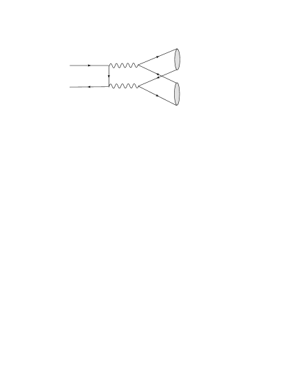
Figure 5: Two photon non-fragmentation diagram. This contribution is suppressed by $\alpha_{em}$ and can be neglected.

There are four different types of diagrams contributing to the production of vector and pseudoscalar meson in $e^{+}e^{-}$ annihilations, to the leading order of the strong and electromagnetic coupling constants. The first type of diagrams contributing to this process are displayed in Fig. 2. These diagrams give the dominant contribution. The diagrams in Fig. 3 contribute to the processes involving $\eta$ and $\eta^{\prime}$, while the diagrams in Fig. 4 only contribute to the processes involving a neutral vector meson, such as $\rho^{0}$, $\omega$ and $\phi$. Although these diagrams are suppressed by $\alpha_{em}$, they can be enhanced by $s/\Lambda_{QCD}^{2}$. This mechanism is similar with the enhancement in penguin-dominated $B$ decays enhancement and the so-called fragmentation mechanism in $e^{+}e^{-}\to VV$ processes fragementation . It is also interesting to explore this effect in $e^{+}e^{-}\to VP$. For $e^{+}e^{-}\to K^{*}K$ and $e^{+}e^{-}\to\rho^{+}\pi^{-}$, the two photon non-fragmentation diagrams can give their contributions as in Fig. 5. But these diagrams suffering the suppression from electromagnetic coupling constant $\alpha_{em}$ which can be neglected safely.

Figure 2: Dominant contribution of $e^{+}e^{-}\to VP$

We begin with a brief review of the PQCD approach. The basic idea of PQCD approach is that it takes into account the transverse momentum of valence quarks which results in the Sudakov factor. The form factor, taking the first diagram in Fig. 2 as an example, can be expressed as the convolution of the wave functions $\psi_{V}$, $\psi_{P}$ and the hard scattering kernel $T_{H}$ by both the longitudinal and the transverse momenta:

$$F_{a}(VP)=\int^{1}_{0}dx_{1}dx_{2}\int d^{2}{\bf{k}}_{T_{1}}d^{2}{\bf{k}}_{T_{2}}\psi_{V}(x_{1},{\bf{k}}_{T_{1}},p_{1},\mu)T_{H}(x_{1},x_{2},Q,{\bf{k}}_{T_{1}},{\bf{k}}_{T_{2}},\mu)\psi_{P}(x_{2},{\bf{k}}_{T_{2}},p_{2},\mu).$$ (31)

Through the Fourier transformation, the above equation can be expressed as:

$$F_{a}(s)=\int^{1}_{0}dx_{1}dx_{2}\int\frac{d^{2}{\bf{b}}_{1}}{(2\pi)^{2}}\frac{d^{2}{\bf{b}}_{2}}{(2\pi)^{2}}{\cal P}_{V}(x_{1},{\bf{b}}_{1},p_{1},\mu)T_{H}(x_{1},x_{2},Q,{\bf{b}}_{1},{\bf{b}}_{2},\mu){\cal P}_{P}(x_{2},{\bf{b}}_{2},p_{2},\mu).$$ (32)

Here ${\cal P}_{i}(x_{j},{\bf{b}}_{j},p_{j},\mu)$ are the Fourier transformation of $\psi_{i}(x_{j},{\bf{k}}_{T_{j}},p_{j},\mu)$, where the subscript $i$ denotes $V$ or $P$, and $j$ indicates $1$ or $2$.

In the above expression, the double logarithms, arising from the overlap of the soft and collinear divergence, have been resummed to result in the Sudakov factor Sudakov

$${{\cal P}_{i}}(x_{j},{\bf{b}}_{j},p_{j},\mu)=\exp\left[-s(x_{j},b_{j},Q)-s(1-x_{j},b_{j},Q)\right]{\bar{\cal P}_{i}}(x_{j},{\bf{b}}_{j},\mu)\;.$$ (33)

The exponent $s(\xi,b_{j},Q)$, $\xi=x_{j}$ or $1-x_{j}$, is expressed as

$$s(\xi,b_{j},Q)=\int_{1/b_{j}}^{\xi Q/\sqrt{2}}\frac{dp}{p}\left[\ln\left(\frac{\xi Q}{\sqrt{2}p}\right)A(\alpha_{s}(p))+B(\alpha_{s}(p))\right]\;,$$ (34)

where the anomalous dimensions $A$ and $B$ to one loop are given by

$$A = {C}_{F}\frac{\alpha_{s}}{\pi},\,\,\,B=\frac{2}{3}\frac{\alpha_{s}}{\pi}\ln\left(\frac{e^{2\gamma_{E}-1}}{2}\right)\;,$$ (35)

with $C_{F}={N_{c}^{2}-1\over 2N_{c}}$ and $\gamma_{E}$ being the Euler constant. The one-loop running coupling constant,

$$\frac{\alpha_{s}(\mu)}{\pi}=\frac{4}{\beta_{0}\ln(\mu^{2}/\Lambda_{QCD}^{2})}\;,$$ (36)

with the coefficients

$$\beta_{0}=\frac{33-2n_{f}}{3},$$ (37)

where $n_{f}$ is the number of the active quark number. We require the relation of the involved scales $\xi Q/\sqrt{2}>1/b_{j}>\Lambda$ as indicated by the bounds of the variable $p$ in Eq. (34). The QCD dynamics below $1/b_{j}$ scale is regarded as being nonperturbative which can be absorbed into the initial condition ${\bar{\cal P}_{i}}(x_{j},{\bf{b}}_{j},\mu)$.

The form factor, as a physical observable, is independent of renormalization scale $\mu$, but the functions ${\bar{\cal P}}$ and $T_{H}$ still contain single logarithms from ultraviolet divergences, which can be summed using the renormalization group equation method. This renormalization group analysis applied to $T_{H}$ gives

$${T_{H}}(x_{j},{\bf{b}}_{j},Q,\mu) = \exp\left[-4\,\int_{\mu}^{t}\frac{d\bar{\mu}}{\bar{\mu}}\gamma_{q}(\alpha_{s}(\bar{\mu}))\right]\times{T_{H}}(x_{j},{\bf{b}}_{j},Q,t)\;,$$ (38)

where $\gamma_{q}=-\alpha_{s}/\pi$ is the quark anomalous dimension in axial gauge and $t$ is the largest mass scale involved in the hard scattering,

$${t=\max(\sqrt{x_{2}}Q,1/b_{1},b_{2})}.$$ (39)

The scale $\sqrt{x_{2}}Q$ is associated with the longitudinal momentum of the quark propagator and $1/b_{j}$ with the transverse momentum. The large-$b_{j}$ behavior of $\cal P$ is summarized as

$${\cal P}_{i}(x_{j},{\bf{b}}_{j},p_{j},\mu) = \exp\left[-s(x_{j},b_{j},Q)-s(1-x_{j},b_{j},Q)-2\int_{1/b_{j}}^{\mu}\frac{d\bar{\mu}}{\bar{\mu}}\gamma_{q}(\alpha_{s}(\bar{\mu}))\right]\times{\bar{\cal P}}_{i}(x,{\bf{b}}_{j},1/b_{j}),\;$$ (40)

where ${\bar{\cal P}}_{i}(x_{j},{\bf{b}}_{j},1/b_{j})$ is the wave function discussed above:

$${\bar{\cal P}}_{i}(x_{j},{\bf{b}}_{j},1/b_{j})=\phi(x_{j},1/b_{j})\times\Sigma({\bf{b}}_{j}).$$ (41)

The threshold resummation threshold ; thresholdB can also play an important role in $e^{+}e^{-}\to VP$ processes. The lowest-order diagrams Fig. 2(a) and (d) give an amplitude proportional to $1/(x_{2}^{2}(1-x_{1}))$ and $1/(x_{2}^{2}x_{1})$ respectively. In the threshold region with $x_{2}\to 0$ (to be precise, $x_{2}\sim O(\Lambda_{QCD}^{2}/s)$), additional collinear divergences are associated with the internal quark. The QCD loop correction to the electromagnetic vertex can produce the double logarithm $\alpha_{s}\ln^{2}x_{2}$ and resummation of this type of double logarithms lead to the Sudakov factor $S_{t}(x_{2})$. Similarly, resummation of $\alpha_{s}\ln^{2}x_{1}$ due to loop corrections in the other diagrams lead to the Sudakov factor $S_{t}(x_{1})$. The Sudakov factor from threshold resummation is universal, independent of flavors of internal quarks, twists, and the specific processes. To simplify the analysis, the following parametrization has been used thresholdB :

$$S_{t}(x)=\frac{2^{1+2c}\Gamma(3/2+c)}{\sqrt{\pi}\Gamma(1+c)}[x(1-x)]^{c}\;,$$ (42)

with the parameter $c=0.3$. This parametrization, symmetric under the interchange of $x$ and $1-x$, is convenient for evaluation of the amplitudes. It is obvious that the threshold resummation modifies the end-point behavior of the meson distribution amplitudes, rendering them vanish faster at $x\to 0$.

Combing all the above ingredients, we obtain the factorization formula for the contribution from Fig. 2(a):

$$F_{a}(VP) = 16\pi C_{F}Qr_{1}\int_{0}^{1}dx_{1}dx_{2}\int_{0}^{\infty}b_{1}db_{1}b_{2}db_{2}$$ (43)

$$\times\phi_{P}^{A}(x_{2},b_{2})[\phi_{V}^{p}(x_{1},b_{1})-\phi_{V}^{v}(x_{1},b_{1})]E(t_{a})h(1-x_{1},x_{2},b_{1},b_{2}),$$

where $h$ and $E$ are defined by PQCDBdecay

$$h(x_{1},x_{2},b_{1},b_{2}) = (\frac{i\pi}{2})^{2}S_{t}(x_{2})\Big{[}\theta(b_{1}-b_{2})H_{0}^{(1)}(\sqrt{x_{2}}Qb_{1})J_{0}(\sqrt{x_{2}}Qb_{2})$$ (44)

$$\;\;+\theta(b_{2}-b_{1})H_{0}^{(1)}(\sqrt{x_{2}}Qb_{2})J_{0}(\sqrt{x_{2}}Qb_{1})\Big{]}H_{0}^{(1)}(\sqrt{x_{1}x_{2}}Qb_{1}),$$

$$E(t_{a}) = \alpha_{s}(t_{a})\mbox{exp}[-S_{1}(t_{a})-S_{2}(t_{a})],$$ (45)

where $J_{0}$ and $H_{0}^{(1)}$ are the Bessel functions, respectively, $t_{a}=\max(\sqrt{x_{2}}Q,1/b_{1},1/b_{2})$ and $r_{1}=M_{V}/Q$.

Similarly, for the other diagrams, the amplitudes are:

$$F_{b}(VP) = -16\pi C_{F}Q\int_{0}^{1}dx_{1}dx_{2}\int_{0}^{\infty}b_{1}db_{1}b_{2}db_{2}E(t_{b})h(x_{2},1-x_{1},b_{2},b_{1})$$ (46)

$$\times\Big{\{}r_{1}(x_{1}-1)[\phi_{1}^{p}(x_{1},b_{1})+\phi_{1}^{v}(x_{1},b_{1})]\phi_{2}^{A}(x_{2},b_{2})+2r_{2}\phi_{1}^{T}(x_{1},b_{1})\phi_{2}^{P}(x_{2},b_{2})\Big{\}},$$

$$F_{c}(VP) = -16\pi C_{F}Q\int_{0}^{1}dx_{1}dx_{2}\int_{0}^{\infty}b_{1}db_{1}b_{2}db_{2}E(t_{c})h(1-x_{2},x_{1},b_{2},b_{1})$$ (47)

$$\times[r_{1}x_{1}(\phi_{1}^{p}(x_{1},b_{1})-\phi_{1}^{v}(x_{1},b_{1}))\phi_{2}^{A}(x_{2},b_{2})+2r_{2}\phi_{1}^{T}(x_{1},b_{1})\phi_{2}^{P}(x_{2},b_{2})],$$

$$F_{d}(VP) = -16\pi C_{F}Qr_{1}\int_{0}^{1}dx_{1}dx_{2}\int_{0}^{\infty}b_{1}db_{1}b_{2}db_{2}E(t_{d})h(x_{1},1-x_{2},b_{1},b_{2})$$ (48)

$$\times(\phi_{1}^{p}(x_{1})+\phi_{1}^{v}(x_{1}))\phi_{2}^{A}(x_{2},b_{2}),$$

with $r_{2}=m_{0}/Q$. The factorization scales $t_{i}$ are chosen as

$$t_{b}=\max(\sqrt{1-x_{1}}Q,1/b_{1},1/b_{2}),\;\;\;t_{c}=\max(\sqrt{x_{1}}Q,1/b_{1},1/b_{2}),\;\;t_{d}=\max(\sqrt{1-x_{2}}Q,1/b_{1},1/b_{2}).$$ (49)

If the final state meson is not $K^{*}$ or $K$, the distribution amplitudes are completely symmetric or antisymmetric under the interchange of $x_{j}$ and $1-x_{j}$. Then one can easily obtain:

$$F_{a}(VP)=F_{d}(VP),\;\;\;F_{b}(VP)=F_{c}(VP).$$ (50)

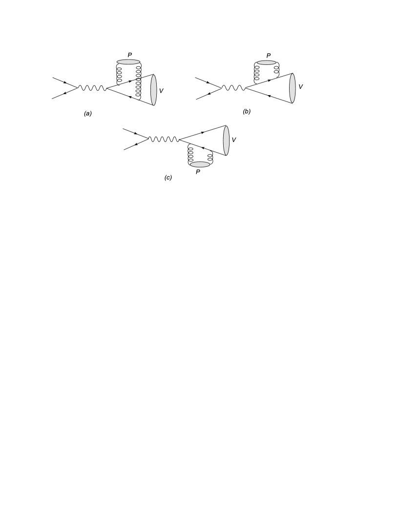
Figure 3: Gluonic contributions

For the flavor-singlet pseudoscalar meson $\eta$ and $\eta^{\prime}$, there are additional contributions from the two-gluon diagrams as displayed in Fig. 3, even if they may be suppressed by the gluonic distribution amplitudes. However, it is still worthwhile to investigate the numerical contribution in order to make our calculations as complete as possible. The computations of these diagrams are much similar with that showed in Fig. 2. The explicit calculations show that the Fig. 3 (a) does not contribute to the transition amplitude, due to the antisymmetry of the two gluons. The amplitudes of the other two diagrams are given as

$$F_{e}(V\eta_{s}) = -8\pi Qr_{1}\frac{f_{s}C_{F}^{2}\sqrt{2N_{c}}}{3(N_{c}^{2}-1)}\int_{0}^{1}dx_{1}dx_{2}\int_{0}^{\infty}b_{1}db_{1}b_{2}db_{2}E(t_{e})h(x_{2},x_{1},b_{1},b_{2})$$ (51)

$$\times[(x_{2}+1)\phi_{V}^{v}(x_{1},b_{1})-(x_{2}-1)\phi_{V}^{p}(x_{1},b_{1})]\frac{\phi_{s}^{G}(x_{2},b_{2})}{x_{2}(1-x_{2})},$$

$$\ \ F_{f}(V\eta_{s}) = 8\pi Qr_{1}\frac{f_{s}C_{F}^{2}\sqrt{2N_{c}}}{3(N_{c}^{2}-1)}\int_{0}^{1}dx_{1}dx_{2}\int_{0}^{\infty}b_{1}db_{1}b_{2}db_{2}E(t_{f})h(1-x_{2},1-x_{1},b_{1},b_{2})$$ (52)

$$\times(x_{1}-1)[(x_{2}-2)\phi_{V}^{v}(x_{1},b_{1})-x_{2}\phi_{V}^{p}(x_{1},b_{1})]\frac{\phi_{s}^{G}(x_{2},b_{2})}{x_{2}(1-x_{2})},$$

for $e^{+}e^{-}\to V\eta_{s}$ process with

$$t_{e}=\max(\sqrt{x_{1}}Q,1/b_{1},1/b_{2}),\;\;\;t_{f}=\max(\sqrt{1-x_{1}}Q,1/b_{1},1/b_{2}).$$ (53)

It should be pointed out that the factor “2” from the exchange of two identical gluons in the final states has been added in the above equations. The amplitude for $e^{+}e^{-}\to V\eta_{n}$ can be easily obtained by replacing the corresponding decay constant with an additional factor $\sqrt{2}$ from Eq. (51,52).

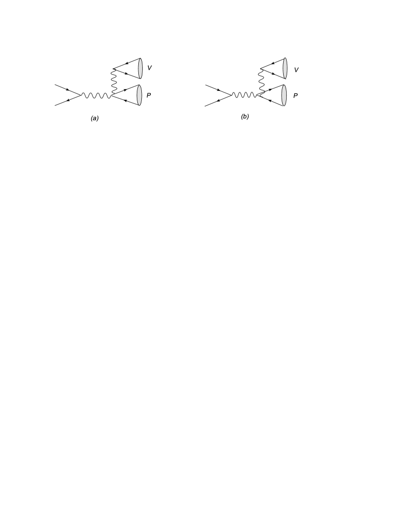
Figure 4: Enhanced diagrams for a neutral vector meson production

Furthermore, there are also contributions from the transition of photon radiated from one valence quark in pseudoscalar meson into vector meson directly, which have been presented in Fig. 4. Although these diagrams maybe suppressed by coupling constant of electromagnetic interactions, they are also enhanced by the almost on-shell photon propagator compared with the first type diagrams, especially for the processes with a very large center mass energy. These diagrams can also be calculated according to $k_{T}$ factorization, however, we will simply adopt collinear factorization due to disappearance of infrared divergence for these two diagrams. These two amplitudes are equal after integrating the momentum fractions carried by the valence quark of the meson. Hence, we obtain the amplitudes corresponding to them as follows:

$$F_{g}(VP) = F_{h}(VP)=\frac{12\pi\alpha_{em}f_{V}f_{P}}{M_{V}s}(1+a_{2}^{P}).$$ (54)

The form factors for the explicit channels can be easily obtained from the combinations of the eight amplitudes $F_{a-h}$. To be more specific, we can write them as

$$F_{\rho^{+}\pi^{-}} = \frac{1}{3}[F_{a}(\rho\pi)+F_{b}(\rho\pi)],$$ (55)

$$F_{\rho^{0}\pi^{0}} = \frac{1}{3}[F_{a}(\rho\pi)+F_{b}(\rho\pi)]+\frac{1}{6}[F_{g}(\rho\pi)+F_{h}(\rho\pi)],$$ (56)

$$F_{\omega\pi^{0}} = [F_{a}(\omega\pi)+F_{b}(\omega\pi)]+\frac{1}{18}[F_{g}(\rho\pi)+F_{h}(\rho\pi)],$$ (57)

$$F_{\phi\pi^{0}} = -\frac{\sqrt{2}}{18}[F_{g}(\phi\pi)+F_{h}(\phi\pi)],$$ (58)

$$F_{K^{*+}K^{-}} = \frac{2}{3}[F_{a}(K^{*}K)+F_{b}(K^{*}K)]-\frac{1}{3}[F_{c}(K^{*}K)+F_{d}(K^{*}K)],$$ (59)

$$F_{K^{*0}\bar{K}^{0}} = -\frac{1}{3}[F_{a}(K^{*}K)+F_{b}(K^{*}K)]-\frac{1}{3}[F_{c}(K^{*}K)+F_{d}(K^{*}K)].$$ (60)

The form factor of $e^{+}e^{-}\to\rho\eta^{(^{\prime})}$ can be written as the combination of its $\bar{n}n$ and $\bar{s}s$ component:

$$F_{V\eta}=\mbox{cos}\theta F_{V\eta_{n}}-\mbox{sin}\theta F_{V\eta_{s}},$$ (61)

$$F_{V\eta^{\prime}}=\mbox{sin}\theta F_{V\eta_{n}}+\mbox{cos}\theta F_{V\eta_{s}},$$ (62)

where $V=\rho^{0},\omega,\phi$ and

$$F_{\rho^{0}\eta_{n}} = [F_{a}(\rho\eta_{n})+F_{b}(\rho\eta_{n})]+\frac{1}{\sqrt{2}}[F_{e}(\rho\eta_{n})+F_{f}(\rho\eta_{n})]+\frac{5}{18}[F_{g}(\rho\eta_{n})+F_{h}(\rho\eta_{n})],$$ (63)

$$\ \ F_{\rho^{0}\eta_{s}} = \frac{1}{\sqrt{2}}[F_{e}(\rho\eta_{s})+F_{f}(\rho\eta_{s})]-\frac{\sqrt{2}}{6}[F_{g}(\rho\eta_{s})+F_{h}(\rho\eta_{s})],$$ (64)

$$\ \ \ \ \ \ \ \ \ F_{\omega\eta_{n}} = \frac{1}{3}[F_{a}(\omega\eta_{n})+F_{b}(\omega\eta_{n})]+\frac{\sqrt{2}}{6}[F_{e}(\omega\eta_{n})+F_{f}(\omega\eta_{n})]+\frac{5}{54}[F_{g}(\omega\eta_{n})+F_{h}(\omega\eta_{n})],$$ (65)

$$\ \ \ \ \ \ \ \ \ \ F_{\omega\eta_{s}} = \frac{\sqrt{2}}{6}[F_{e}(\omega\eta_{s})+F_{f}(\omega\eta_{s})]-\frac{\sqrt{2}}{18}[F_{g}(\omega\eta_{s})+F_{h}(\omega\eta_{s})],$$ (66)

$$\ \ \ \ \ \ \ \ \ F_{\phi\eta_{n}} = -\frac{1}{3}[F_{e}(\phi\eta_{n})+F_{f}(\phi\eta_{n})]-\frac{5\sqrt{2}}{54}[F_{g}(\phi\eta_{n})+F_{h}(\phi\eta_{n})],$$ (67)

$$\ \ \ \ \ \ F_{\phi\eta_{s}} = -\frac{2}{3}[F_{a}(\phi\eta_{s})+F_{b}(\phi\eta_{s})]-\frac{1}{3}[F_{e}(\phi\eta_{s})+F_{f}(\phi\eta_{s})]-\frac{1}{27}[F_{g}(\phi\eta_{s})+F_{h}(\phi\eta_{s})].$$ (68)

III Numerical results and discussions

III.1 Cross section

Making use of the distribution amplitudes and the inputs listed before, one can easily obtain the cross sections for the process $e^{+}e^{-}\to PV$. Here we would like to present the results of cross sections at $\sqrt{s}$ =3.67 GeV and 10.58 GeV in Table 2 together with the data measured by CLEO-c and BaBar collaboration. The different scenarios S1, S2, S3 denoting different transverse momentum distribution functions, which will be discussed in the next subsection. As the longitudinal decay constants of the vector mesons and the pseudoscalar meson decay constants are precisely determined, the uncertainties from these inputs are neglected. Therefore the uncertainties shown in Table 2 are from the transverse decay constants of the vector meson shown in table 1.

From the Eqs. (55) and (56), we can see that, if neglecting the fragmentation contribution $F_{g,h}$, the cross sections for production of $\rho^{+}\pi^{-}$ and $\rho^{0}\pi^{0}$ in $e^{+}e^{-}$ annihilation should be the same. At $\sqrt{s}=3.67$ GeV, the fragmentation can not give large contribution as the on-shellness enhancement is not strong. Thus theoretical calculation predicts that the ratio $R_{1}=\frac{\sigma(e^{+}e^{-}\to\rho^{+}\pi^{-})}{\sigma(e^{+}e^{-}\to\rho^{0}\pi^{0})}$ should be around 1. From table 2, one can see that this prediction is consistent with the CLEO-c results. At higher energies, the enhancement effect becomes more important. This effect can weaken $e^{+}e^{-}\to\rho^{0}\pi^{0}$ by about ten percents at $\sqrt{s}=10.58$ GeV, relative to $e^{+}e^{-}\to\rho^{+}\pi^{-}$. If the center mass energy is large enough, the contribution from diagrams in Fig. 4 will be dominant over the other contributions.

Table 2: Results of $e^{+}e^{-}\to VP$ cross sections at $\sqrt{s}=3.67$ GeV and $\sqrt{s}=10.58$ GeV using three different transverse momentum distribution functions, denoted as S1, S2 and S3 respectively. The experimental results from CLEO-c and BaBar collaborations are also included.

	$\sqrt{s}=3.67$ GeV				$\sqrt{s}=10.58$ GeV
Channel	$\sigma_{S1}$(pb)	$\sigma_{S2}$(pb)	$\sigma_{S3}$(pb)	$\sigma_{exp}$(pb)	$\sigma_{S1}$(fb)	$\sigma_{S2}$(fb)	$\sigma_{S3}$(fb)	$\sigma_{exp}$(fb)
$\rho^{+}\pi^{-}$	$3.8^{+0.3}_{-0.2}$	$1.9^{+0.1}_{-0.2}$	$2.9^{+0.2}_{-0.2}$	$4.8^{+1.5+0.5}_{-1.2-0.5}$	$0.71^{+0.04}_{-0.04}$	$0.55^{+0.03}_{-0.03}$	$0.68^{+0.04}_{-0.04}$
$\rho^{0}\pi^{0}$	$3.8^{+0.3}_{-0.2}$	$1.9^{+0.1}_{-0.2}$	$2.9^{+0.2}_{-0.2}$	$3.1^{+1.0+0.4}_{-0.8-0.4}$	$0.64^{+0.04}_{-0.04}$	$0.50^{+0.04}_{-0.03}$	$0.62^{+0.04}_{-0.03}$
$\omega\pi^{0}$	$28.2^{+2.2}_{-2.2}$	$13.8^{+1.1}_{-1.1}$	$21.2^{+1.7}_{-1.6}$	$15.2^{+2.8+1.5}_{-2.4-1.5}$	$5.2^{+0.4}_{-0.3}$	$4.1^{+0.5}_{-0.3}$	$5.0^{+0.4}_{-0.3}$
$\phi\pi^{0}$	$1.2\times 10^{-4}$	$1.2\times 10^{-4}$	$1.2\times 10^{-4}$	$<2.2$	$2.1\times 10^{-3}$	$2.1\times 10^{-3}$	$2.1\times 10^{-3}$
$K^{*+}K^{-}$	$5.6^{+0.4}_{-0.4}$	$2.9^{+0.1}_{-0.3}$	$4.3^{+0.3}_{-0.3}$	$1.0^{+1.1+0.5}_{-0.7-0.5}$	$1.2^{+0.02}_{-0.02}$	$0.83^{+0.05}_{-0.05}$	$1.1^{+0.0}_{-0.1}$
$K^{*0}\bar{K}^{0}$	$34.8^{+2.4}_{-2.3}$	$17.3^{+1.2}_{-1.1}$	$26.4^{+1.8}_{-1.8}$	$23.5^{+4.6+3.1}_{-3.9-3.1}$	$7.1^{+0.4}_{-0.4}$	$5.6^{+0.2}_{-0.4}$	$6.8^{+0.4}_{-0.4}$
$\rho^{0}\eta$	$16.6^{+0.9}_{-1.0}$	$8.1^{+0.5}_{-0.4}$	$12.5^{+0.7}_{-0.7}$	$10.0^{+2.2+1.0}_{-1.9-1.0}$	$3.3^{+0.2}_{-0.2}$	$2.4^{+0.2}_{-0.1}$	$3.1^{+0.2}_{-0.2}$
$\rho^{0}\eta^{\prime}$	$8.6^{+0.6}_{-0.5}$	$4.3^{+0.3}_{-0.3}$	$6.6^{+0.4}_{-0.4}$	$2.1^{+4.7+0.2}_{-1.6-0.2}$	$2.1^{+0.1}_{-0.1}$	$1.5^{+0.1}_{-0.0}$	$2.0^{+0.1}_{-0.1}$
$\omega\eta$	$1.5^{+0.1}_{-0.1}$	$0.76^{+0.03}_{-0.07}$	$1.1^{+0.1}_{-0.1}$	$2.3^{+1.8+0.5}_{-1.0-0.5}$	$0.31^{+0.02}_{-0.02}$	$0.22^{+0.02}_{-0.01}$	$0.29^{+0.02}_{-0.01}$
$\omega\eta^{\prime}$	$0.79^{+0.06}_{-0.06}$	$0.39^{+0.03}_{-0.03}$	$0.60^{+0.04}_{-0.04}$	$<17.1$	$0.20^{+0.01}_{-0.02}$	$0.14^{+0.01}_{-0.01}$	$0.18^{+0.012}_{-0.01}$
$\phi\eta$	$19.1^{+1.1}_{-1.1}$	$9.6^{+0.6}_{-0.6}$	$14.6^{+0.8}_{-0.9}$	$2.1^{+1.9+0.2}_{-1.2-0.2}$	$4.3^{+0.2}_{-0.2}$	$3.3^{+0.2}_{-0.2}$	$4.1^{+0.1}_{-0.2}$	$2.9^{+0.5+0.1}_{-0.5-0.1}$
$\phi\eta^{\prime}$	$22.6^{+1.4}_{-1.3}$	$11.5^{+0.8}_{-0.7}$	$17.4^{+1.1}_{-1.0}$	$<12.6$	$5.8^{+0.3}_{-0.3}$	$4.4^{+0.2}_{-0.3}$	$5.4^{+0.4}_{-0.3}$

The process $e^{+}e^{-}\to K^{*}K$ has previously been calculated in PQCD ($k_{T}$ factorization) and has been shown to give correct order of magnitude for the form factors CKM05 . But they assume SU(3) symmetry using asymptotic wave functions. In order to show the $SU(3)$ symmetry breaking effect in $e^{+}e^{-}\to K^{*}K$, we define the ratio:

$$R_{2}=\frac{\sigma(e^{+}e^{-}\to K^{*0}\bar{K}^{0})}{\sigma(e^{+}e^{-}\to K^{*+}K^{-})}=\bigg{|}\frac{1+\frac{F_{c}+F_{d}}{F_{a}+F_{b}}}{2-\frac{F_{c}+F_{d}}{F_{a}+F_{b}}}\bigg{|}^{2}.$$ (69)

If we assume that $SU(3)$ symmetry works well, then the light cone distribution amplitude of $K$ and $K^{*}$ is completely symmetric under the exchange of the momentum fractions of quark and anti-quark. We will have $F_{a}+F_{b}=F_{c}+F_{d}$, then $R_{2}=4$ can be derived directly from Eq. (59) and (60). One of the SU(3) symmetry breaking effects is that the $s$ quark is heavier than $n(=u,d)$ quark and carries more momentum in the final state light $K^{(*)}$ meson. The gluon which generates $\bar{s}s$ is harder than the $\bar{n}n$ generator, then the former coupling constant is smaller due to the more off-shell gluon. Consequently this leads to a smaller contribution to the form factor $|F_{a}+F_{b}|$ than $|F_{c}+F_{d}|$. Therefore $R_{2}$ is larger than 4. Using the cross sections listed in Table 2, we obtain our result for $R_{2}$:

$$R_{2}=6.0,$$ (70)

where only the central value is given. The CLEO-c results indicate that there is a large deviation from the $SU(3)$ limit ExpVP3 :

$$R_{2}=23.5^{+17.1}_{-26.1}\pm 12.2.$$ (71)

The central value of the experimental results for $R_{2}$ seems too large, but as the uncertainties are also large, our result could be consistent with results from CLEO-c collaboration.

For the processes involving $\eta^{(^{\prime})}$ such as the process $e^{+}e^{-}\to\phi\eta$, we find that the gluonic contribution is around one percent to the total cross section at $\sqrt{s}=10.58$ GeV. This conclusion is consistent with the study on the $B\to\eta^{(^{\prime})}$ form factor GluonicCKL . The cross sections of $e^{+}e^{-}\to\rho(\omega)\eta^{(\prime)}$ and $\omega\pi^{0}$ at $\sqrt{s}=3.67$ GeV calculated in $k_{T}$ factorization are consistent with the experimental values. The result for $e^{+}e^{-}\to\phi\eta$ at $\sqrt{s}=10.58$ GeV is also consistent with experimental data. This indicates that $k_{T}$ factorization is an effective method to deal with the infrared divergences in exclusive processes.

The measurement of cross sections at different center mass energy $\sqrt{s}$ can shed light on the $s$ dependence. This dependence is expected as $1/s^{3}$ sdependence3 or $1/s^{4}$pQCDBL ; sdependence4 . Our results displayed in Table 2 at two different scales $\sqrt{s}=10.58$ GeV and 3.67 GeV seem to favor the $1/s^{3}$ scaling. It should be noticed that we neglected the $Q=\sqrt{s}$ dependence of the light cone wave function and next-to-leading order contributions in our calculation. Therefore the $s$ dependence study of the cross sections is not a complete one.

As the quark or the gluon could be on-shell, we expect the amplitudes receive an imaginary part which is similar with the exclusive $B$ decays PQCDBdecay ; Bdecayversus . The imaginary part in $e^{+}e^{-}\to\phi\eta$ at $\sqrt{s}=10.58$ GeV is about twice as large as the real part in magnitude and a large strong phase is consequently generated. The contributions from Fig. 3 are small; Contributions from Fig. 4 are small and real; The four diagrams in Fig. 2 give comparable contributions which are the main origin of the imaginary part. Unlike the B decays, strong phase here does not make any physical meaning, since there is no electroweak phase for interference.

From Table 2, we can see that at $\sqrt{s}=10.58$ GeV, the cross sections for many processes, especially $e^{+}e^{-}\to K^{0*}\bar{K}^{0}$ and $e^{+}e^{-}\to\phi\eta^{\prime}$, are large enough to be detected. We suggest the experimentalists to measure these channels.

In the above, we only concentrate on the exclusive production of a vector and a pseudoscalar. Applications to $PP$ and $VV$ productions are straightforward. The diagrams in Fig. 2 will give dominant contributions, where the final state must have negative charge conjugation quantum number $C=-1$. Then only three channels for $PP$ is allowed through one photon annihilation: $e^{+}e^{-}\to\pi^{+}\pi^{-}$, $e^{+}e^{-}\to K^{+}K^{-}$ and $e^{+}e^{-}\to K^{0}\bar{K}^{0}$. If $U$-spin is well respected, $d$ and $s$ quarks are symmetric in $K^{0}$ and the cross section of $e^{+}e^{-}\to K^{0}\bar{K}^{0}$ is zero. The non-zero result for $e^{+}e^{-}\to K^{0}\bar{K}^{0}$ can reflect the size of $U$-spin symmetry breaking. For production of $VV$, the analysis is similar. Two flavor singlet vector mesons can not be produced through one photon annihilation diagrams either, but these productions could receive large additional contributions fragementation .

III.2 Theoretical Uncertainties

One of the major uncertainties in our computations comes from the distribution amplitudes for the pseudoscalar and vector mesons. The dependence on the longitudinal distribution amplitudes has been studied intensively in the exclusive B decays Kurimuto . They will give 10-20% uncertainties here too. In the following, we will focus on the transverse momentum distribution. In PQCD approach, the intrinsic transverse momentum is taken into account. The resummation of large double logarithms results in the Sudakov factor which suppresses the large $b$ region’s contribution. As we can see from Eq. (28), the transverse momentum distribution function also suppress the contribution from the large $b$ region. For momentum transfer of a few GeV, the transverse momentum distribution function damps more than the Sudakov factor transverseDA . This suppression makes PQCD approach more self-consistent. So we expect that there is an obvious suppression for the production rate of $e^{+}e^{-}\to VP$ at $\sqrt{s}=3.67$ GeV if the transverse momentum distribution amplitude is taken into account. However, at present, it is still lack of first-principle study on the intrinsic transverse momentum distribution. The simple form is chosen as the Gaussian form discussed in Eq. (28) or the following one,

$$\Sigma(x,b)=\mbox{exp}\left[-\frac{x(1-x)b^{2}}{4a^{2}}\right],$$ (72)

where $a$ is the transverse size parameter as $\beta$. As a simple test, we can choose $a=1$ which is consistent with the value used in Kurimuto . Comparing with the form in Eq. (28), we can see that at $x=1/2$, the two different forms coincides. But for small or large $x$, the second form can not give the same strong suppression as the first form (Eq. (28)). We can expect the suppression of the results of taking the second form is less effective than the first one. In Table 2, we give three different kinds of results: without the intrinsic momentum distribution (denoted as S1), i.e. $\Sigma=1$; with the first distribution as Eq. (28) (denoted as S2); with the second kind as Eq. (72) (denoted as S3). Comparing the different results in Table 2, we find that at small center mass energy $\sqrt{s}=3.67$ GeV the suppression from transverse momentum distribution is more effective: the suppression is $50\%$ for S2 and $20\%$ for S3. Since the results depend on the explicit form of transverse momentum distribution, more experimental results are needed.

In this calculation, we only present the leading order calculations. The complete next-to-leading order calculations are much more complicated NLO . For a simple estimate of the size of the next-to-leading order contribution, we use the traditional method varying $\Lambda_{QCD}$ and factorization scale $t$ in Eq. (39), (49) and (53): $\Lambda_{QCD}=(0.25\pm 0.05)$ GeV; changing hard scale $t$ from $0.75t$ to $1.25t$ (not changing $1/b_{i}$). We find that our results are not sensitive to these changes. This implies that the next-to-leading order contribution is probably not very large.

IV Conclusions

In this paper, we have studied the exclusive processes $e^{+}e^{-}\to VP$ in PQCD approach based on the $k_{T}$ factorization. We give three different kinds of results corresponding to different transverse momentum distribution functions. With the proper distribution function, our results can be consistent with the experimental results. The two different transverse momentum distribution functions S2 and S3 can give about $50\%$ and $20\%$ suppression respectively at center mass energy $\sqrt{s}=3.67\rm{{GeV}}$. We have included the gluonic contribution for the processes involving $\eta^{(^{\prime})}$ meson whose effect is found tiny. We have also included the contribution in which the flavor singlet vector meson is produced by an additional photon. This contribution could be neglected at center mass energy $\sqrt{s}=3.67\rm{{GeV}}$, while these diagrams could induce about $10\%$ difference between $e^{+}e^{-}\to\rho^{0}\pi^{0}$ and $e^{+}e^{-}\to\rho^{+}\pi^{-}$ at $\sqrt{s}=10.58$ GeV. The $s$ dependence of the cross section has been directly studied which indicates that the $1/s^{3}$ scaling is more favored than $1/s^{4}$.

References

• (1) G.P. Lepage and S.J. Brodsky, Phys. Rev. Lett. 43, 545(1979); (E) 43, 1625 (1979); Phys. Lett. B87, 359(1979); Phys. Rev. D22, 2157(1980); S.J. Brodsky and G.P. Lepage, Phys. Rev. D24, 2848(1981).
• (2) A.V. Efremov and A.V. Radyushkin, Phys. Lett. B94, 245(1980); V.V. Braguta, A.K. Likhoded, A.V. Luchinsky, Phys. Rev. D72, 074019 (2005); Phys. Lett. B635, 299 (2006)
• (3) A.V. Manohar and I.W. Stewart, arXiv:hep-ph/0605001.
• (4) H.N. Li and G. Stermann, Nucl. Phys. B381, 129(1992).
• (5) H.N. Li and H.L. Yu, Phy. Rev. Lett. 74, 4388(1995); Y.Y. Keum, H.N. Li and A.I. Sanda, Phys. Lett. B504, 6(2001); Phys. Rev. D63, 054008(2001); C.D. LΓΌ, K. Ukai and M.Z. Yang, Phys. Rev. D63, 074009(2001); D.S. Du, C.H. Huang, Z.T. Wei and M.Z. Yang, Phys. Lett. B520, 50(2001); C.D. LΓΌ and M.Z. Yang, Eur. Phys. J.C23, 275(2002); A. Ali, et al., arXiv: hep-ph/0703162.
• (6) M. Ablikim, Phys. Rev. D70,112007(2004).
• (7) N.E. Adam, et al., CLEO Collaboration, Phys. Rev. Lett. 94, 012005(2005).
• (8) G.S. Adams, et al., CLEO Collaboration, Phys. Rev. D73, 012002(2006).
• (9) B. Aubert, et al., BaBar Collaboration, Phys. Rev. D74, 111103(2006).
• (10) For an explicit discussion of the similarity of $e^{+}e^{-}$ annihilation and the annihilation diagrams in $B$ decays, please see the talk given by A. Kagan at 4th International Workshop on the CKM Unitarity Triangle (CKM 2006), Nagoya, Japan, 12-16 Dec 2006.
• (11) Particle Data Group, W.-M. Yao et al., J. Phys. G 33,1 (2006).
• (12) P. Ball and R. Zwicky, Phys. Rev. D71, 014029 (2005).
• (13) P.Β Ball and R.Β Zwicky, JHEP 0604, 046(2006) [hep-ph/0603232].
• (14) V.L. Chernyak and A.R. Zhitnitsky, Phys. Rept. 112, 173 (1984); V.M. Braun and I.E. Filyanov, Z. Phys. C 44, 157 (1989); P. Ball, JHEP 9809, 005 (1998); V.M. Braun and I.E. Filyanov, Z. Phys. C 48, 239 (1990); A.R. Zhitnitsky, I.R. Zhitnitsky and V.L. Chernyak, Sov. J. Nucl. Phys. 41, 284(1995), Yad. Fiz. 41, 445 (1985); P.Ball, JHEP 9901, 010(1999).
• (15) V.M. Braun and A. Lenz, Phys. Rev. D70, 074020; P. Ball and A.N. Talbot, JHEP 0506, 063(2005); P. Ball and R. Zwicky, Phys. Lett. B633, 289(2006); A. Khodjamirian, Th. Mannel and M. Melcher, Phys. Rev.Β D70, 094002(2004); P.Β Ball, V.M.Β Braun, A.Β Lenz, JHEP 0605, 004 (2006)
• (16) A.Β P.Β Bakulev, S.Β V.Β Mikhailov and N.Β G.Β Stefanis, Phys. Lett. B508, 279 (2001); Erratum-ibid. B590, 309 (2004); Phys. Rev. D67, 074012 (2003); Phys. Lett. B578, 91 (2004); S.Β i.Β Nam and H.Β C.Β Kim, Phys. Rev. D74, 076005 (2006)
• (17) T.Β Feldmann, P.Β Kroll and B.Β Stech, Phys. Rev. D58, 114006(1998); Phys. Lett. B449, 339(1999).
• (18) Y.Y.Β Charng, T.Β Kurimoto and H.N.Β Li, Phys. Rev.Β D74, 074024(2006).
• (19) P. Kroll, K. Passek-Kumericki, Phys. Rev. D67, 054017 (2003); A. Ali and A.Y. Parkhomenko, Eur. Phys. J. C30, 183(2003).
• (20) M. V. Terentev, Sov. J. Nucl. Phys. 33, 911(1981) [Yad. Fiz. 33, 1692 (1981)]; T. Ohrndorf, Nucl. Phys. B186, 153(1981); M.A. Shifman and M.I. Vysotsky, Nucl. Phys. B186, 475(1981); V.N. Baier and A.G. Grozin, Nucl. Phys. B192, 476(1981); M. V. Terentev, JETP Lett. 33, 67(1981) [Pisma Zh. Eksp. Teor. Fiz. 33, 71(1981)]; A. V. Belitsky and D. Mueller, Nucl. Phys. B537, 397(1999).
• (21) P. Ball, V.M. Braun, Y. Koike, and K. Tanaka, Nucl. Phys. B529, 323 (1998); P. Ball, V.M. Braun, Nucl. Phys. B543, 201(1999).
• (22) P. Ball, and V. M. Braun, Phys. Rev. D54, 2182(1996); P. Ball, and R. Zwicky, JHEP 0602, 034 (2006); V.M. Braun, and A. Lenz, Phys. Rev. D70, 074020 (2004); P. Ball, and M. Boglione, Phys. Rev. D68, 094006(2003).
• (23) R. Jakob and P.Kroll, Phys. Lett. B315, 463(1993); Erratum-ibid. B319, 545(1993); N.Β G.Β Stefanis, W.Β Schroers and H.Β C.Β Kim, Phys. Lett. B449, 299(1999).
• (24) M. Beneke, J. Rohrer and D. Yang, Phys. Rev. Lett. 96, 141801(2006); C.D. LΓΌ, Y.L. Shen and W.Wang, Chin. Phys. Lett.23, 2684(2006).
• (25) M. Davier, M. Peskin and A. Snyder, arXiv:hep-ph/0606155; G.T. Bodwin, E. Braaten, J. Lee and C. Yu, Phys. Rev. D74, 074014(2006).
• (26) J. Botts and G. Sterman, Nucl. Phys. B325, 62(1989); N.Β G.Β Stefanis, W.Β Schroers and H.Β Ch.Β Kim, Eur. Phys. J. C18, 137 (2000).
• (27) G. Sterman, Phys. Lett. B179, 281(1986); Nucl. Phys. B281, 310(1987); S. Catani and L. Trentadue, Nucl. Phys. B327, 323(1989); Nucl. Phys. B353, 183(1991); H.N. Li, Phys. Lett. B454, 328(1999); Chin. J. Phys.(Taipei) 37, 569(1999).
• (28) H.N. Li, Phys. Rev. D66, 094010(2002).
• (29) talk given by A. Kagan at 3rd International Workshop on the CKM Unitarity Triangle (CKM 2005), San Diego, USA, 15-18 March 2005.
• (30) J.M. Genrard and G. Lopez Castro, Phys. Lett. B425, 365(1998).
• (31) The first paper in Ref.Β PseudoscalarWV ; V.L. Chernyak, hep-ph/9906387.
• (32) Y.Y. Keum and H.n. Li, Phys. Rev.D63,074006(2001).
• (33) T. Kurimoto, Phys. Rev. D74, 014027(2006).
• (34) The $O(\alpha_{s})$ corrections are being studied by S.Nandi and H.N. Li.