LANDAU POTENTIAL STUDY
OF THE CHIRAL PHASE TRANSITION IN A QCD-LIKE THEORY

Abstract

We investigate the chiral phase transition of a QCD-like theory, based the shape change of the effective potential near the critical point. The potential is constructed with the auxiliary field method, and a source term coupled to the field is introduced in order to compute the potential shape numerically. We also generalize the potential so as to have two independent order parameters, the quark scalar density and the number density. We find a tri-critical point locating at $(T,\mu)=(97,203)$ MeV, and visualize it as the merging point of three potential minima.

1 Introduction and Summary

The phase structure of quantum chromodynamics (QCD) at finite temperature $T$ and quark chemical potential $\mu$ is actively investigated in the context of the collider experiments using ultra-relativistic heavy ions, which create the highly-excited QCD matter.[1] The chiral symmetry of QCD, which is spontaneously broken in the vacuum, will be restored at sufficiently high temperature and/or quark chemical potential. We investigate here the chiral phase transition of a QCD-like theory, focusing on the shape change of the effective potential near the critical point. The QCD-like theory is the renormalization-group (RG) improved ladder approximation for the Schwinger-Dyson (SD) equation of QCD.[2, 3, 4] This theory describes the dynamical chiral symmetry breaking, retaining the correct high energy behavior of the quark propagator. Using this theory and the low-density expansion, the pion-nucleon sigma term and the quark condensate at finite density have been calculated successfully.[5]

As for the effective potential, the Cornwall-Jackiw-Tomboulis (CJT) potential functional[6] has been used in several works for the study of dynamical chiral symmetry breaking. However, the interpretation of the CJT potential away from the extremum is not obvious. Thus, in order to investigate the nature of the chiral phase transition through the shape change of the effective potential, we construct the Landau potential[7] of the QCD-like theory[8] by using the auxiliary field method, in which the bilocal external field is introduced. We generalize the potential so as to have two independent order parameters, the quark condensate and the quark number density at fixed $T$ and $\mu$. By plotting the 2D contour map in the order parameter plane, the shape change of the potential near the critical point can be elucidated. We find a tri-critical point is located at $(T,\mu)=(97,203)$ MeV, and visualize it as the merging point of three potential minima.

2 Basic Ingredients of a QCD-Like Theory

2.1 In the vacuum

In the QCD-like theory, first, we neglect the self-interaction between the gluons and integrate out the gluon fields, leaving the non-local interactions between the quark. The non-Abelian nature is taken into account in the running of the coupling constant. The generating functional $Z=\int{\cal D}\psi{\cal D}{\bar{\psi}}{\cal D}A\exp(i\int d^{4}x{\cal L}_{\rm QCD})$ is approximated by $Z\!\!\sim\!\!\int{\cal D}\psi{\cal D}{\bar{\psi}}\exp(i\int d^{4}x{\cal{\widetilde{L}}})$ where

$$\int d^{4}x\mathcal{{\widetilde{L}}} = \int_{p}\overline{\psi}(p)\ \raise 0.43057pt\hbox{$/$}\kern-6.30005pt\hbox{$p$}\ \psi(p)$$ (1)

$$-\frac{i}{2}\int_{pqk}\!\psi_{\alpha}\!\!\left(p-\frac{q}{2}\right)\overline{\psi}_{\beta}\!\!\left(p+\frac{q}{2}\right)K^{\alpha\beta,\gamma\delta}(p,k)\psi_{\gamma}\!\!\left(k+\frac{q}{2}\right)\overline{\psi}_{\delta}\!\!\left(k-\frac{q}{2}\right).$$

Here, $\psi(p)$ is the quark field in the momentum space and $\int_{p}\!\!\equiv\!\!\int d^{4}p/(2\pi)^{4}$. The indices, $\alpha,\beta,\cdots$ correspond to the Dirac structure. We defined the kernel $K$ as

$$K^{\alpha\beta,\gamma\delta}(p,k)=g^{2}(\gamma_{\mu}T^{a})^{\delta\alpha}(\gamma_{\nu}T^{a})^{\beta\gamma}iD^{\mu\nu}(p-k)\ ,$$ (2)

where $T^{a}$ is the color $su(N_{c})$ generator and $iD^{\mu\nu}(p)$ is the gluon propagator:

$$iD^{\mu\nu}(p)=\frac{g^{\mu\nu}-(1-\alpha)p^{\mu}p^{\nu}/p^{2}}{p^{2}}\ .$$ (3)

Hereafter, we employ the Landau gauge, $\alpha=0$. The non-Abelian nature of the gluon interaction is treated in this model as the one-loop running of $g$: $\overline{g}(\textrm{max}(p_{E}^{2},k_{E}^{2}))$ with $p_{E}$ the momentum in Euclidian space. The divergence of $\overline{g}(p_{E}^{2})$ appearing at $p_{E}=\Lambda_{\rm QCD}$ is removed by introducing an infrared cutoff parameter $p_{IF}$ as [9]

$$\overline{g}^{2}(p_{E}^{2})=\frac{2}{a}\frac{1}{\textrm{ln}((p_{E}^{2}+p^{2}_{IF})/\Lambda_{\rm QCD}^{2})}$$ (4)

with $a=1/(8\pi^{2})\cdot(11N_{c}-2N_{f})/3$. Here, $N_{c}(=3)$ and $N_{f}(=2)$ are the numbers of colors and flavors, respectively.

We next introduce the following bilocal auxiliary field for non-perturbative analysis:

$$\chi_{\alpha\beta}(p,q)=\int_{k}K^{\alpha\beta,\gamma\delta}(p,k)\psi_{\gamma}\left(k+\frac{q}{2}\right)\overline{\psi}_{\delta}\left(k-\frac{q}{2}\right).$$ (5)

This makes the action bilinear in the quark fields $\psi$ and $\overline{\psi}$. Then, integrating out $\psi$ and $\overline{\psi}$, we end up with $Z=\int{\cal D}\chi\exp i\,\Gamma[\chi]$ where the classical action reads

$$\Gamma[\chi] = \frac{1}{2}\int_{pkq}\textrm{tr}[\chi(p,-q)K^{-1}(p,k)\chi(k,p)]-i\textrm{Tr Ln}(\ \raise 0.43057pt\hbox{$/$}\kern-6.30005pt\hbox{$p$}\delta^{4}(q)(2\pi)^{4}-\chi(p,-q)).\$$ (6)

In the mean-field approximation the SD equation is obtained as the extremum condition for this classical action for $\chi$. The existence of a non-trivial solution for $\chi$ indicates the dynamical breaking of the chiral symmetry. In the vacuum this solution is expressed as $\langle\chi_{\alpha\beta}\rangle=\Sigma_{\alpha\beta}(p)\delta^{4}(q)(2\pi)^{4}$ with the mass function $\Sigma$, and the effective potential $V[\Sigma]=-\Gamma[\chi]/\int d^{4}x$ becomes

$$V[\Sigma] = -\frac{1}{2}\int_{pk}\textrm{tr}[\Sigma(p)K^{-1}(p,k)\Sigma(k)]+i\int_{p}\textrm{tr ln}(\ \raise 0.43057pt\hbox{$/$}\kern-6.30005pt\hbox{$p$}-\Sigma(p)).$$ (7)

Then the SD equation, $\delta V/\delta\Sigma=0$, in the improved ladder approximation is written

$$\Sigma_{\alpha\beta}(p)=\frac{1}{i}\int_{k}K^{\alpha\beta,\gamma\delta}(p,k)\biggl{(}\frac{1}{\raise 0.6458pt\hbox{$/$}\kern-5.29999pt\hbox{$k$}-\Sigma(k)}\biggr{)}_{\gamma\delta}.$$ (8)

Although the $\Sigma_{\alpha\beta}(p)$ has the general form $\Sigma(p^{2})\delta_{\alpha\beta}+\Sigma_{v}(p^{2})\raise 0.43057pt\hbox{$/$}\kern-6.30005pt\hbox{$p$}_{\alpha\beta}$ in the vacuum, we can set $\Sigma_{v}(p^{2})=0$ in the Landau gauge ($\alpha=0$). After carrying out the Wick rotation and the angle integration, the SD equation becomes

$$\Sigma(p^{2}_{E}) = \frac{3C_{2}(N_{c})}{16\pi^{2}}\int_{0}^{\infty}k_{E}^{2}dk_{E}^{2}\overline{g}^{2}(\textrm{max}(p_{E}^{2},k_{E}^{2}))\frac{1}{\textrm{max}(p_{E}^{2},k_{E}^{2})}\frac{\Sigma(k^{2}_{E})}{k_{E}^{2}+\Sigma(k^{2}_{E})^{2}}\ ,\qquad$$ (9)

where $C_{2}(N_{c})=T^{a}T^{a}=(N_{c}^{2}-1)/2N_{c}$.

2.2 Order parameters

The quark condensate with the four momentum cutoff $\Lambda$ is defined as

$$\langle\overline{\psi}\psi\rangle_{\Lambda} = -\frac{1}{i}\int_{p}\textrm{tr}\left(\frac{1}{\raise 0.43057pt\hbox{$/$}\kern-6.30005pt\hbox{$p$}-\Sigma(k^{2})}\right)=-\frac{N_{c}}{4\pi^{2}}\int^{\Lambda^{2}}_{0}\!\!dp_{E}^{2}\ \frac{p_{E}^{2}\Sigma(p_{E}^{2})}{p_{E}^{2}+\Sigma(p_{E}^{2})^{2}}\ .$$ (10)

This bare value at the scale $\Lambda$ is converted into the value at the lower energy scale $\mu$ (e.g., 1 GeV) via the renormalization group equation

$$\langle\overline{\psi}\psi\rangle_{\mu}=\langle\overline{\psi}\psi\rangle_{\Lambda}\left(\frac{\overline{g}^{2}(\Lambda)}{\overline{g}^{2}(\mu)}\right)^{1/[4((12C_{2}(N_{c}))^{-1}(11N_{c}-2N_{f})/3)]}\ .$$ (11)

Next, the pion decay constant $f_{\pi}$ is estimated in terms of the mass function $\Sigma(p^{2})$ by utilizing the Pagels-Stokar formula:

$$f^{2}_{\pi}=\frac{N_{c}}{4\pi^{2}}\!\int_{0}^{\infty}\!\!\!dp_{E}^{2}\frac{p_{E}^{2}\Sigma(p_{E}^{2})}{(p_{E}^{2}+\Sigma^{2}(p_{E}^{2}))^{2}}\!\left(\!\!\Sigma(p_{E}^{2})\!-\!\frac{p_{E}^{2}}{2}\frac{d\Sigma(p_{E}^{2})}{dp_{E}^{2}}\!\!\right)\ .$$ (12)

We fix the value of $\Lambda_{\rm QCD}$ here so as to reproduce the empirical value of $f_{\pi}$.

2.3 At finite temperature

We use the imaginary time formalism to extend the QCD-like theory to the case with finite temperature and chemical potential, making the following replacement:

$$\int_{p}f(p_{0},\mbox{\boldmath$p$})\longrightarrow T\sum_{n=-\infty}^{\infty}\int\frac{d^{3}\mbox{\boldmath$p$}}{(2\pi)^{3}}f(i\omega_{n}+\mu,\mbox{\boldmath$p$})\ ,$$ (13)

where $\omega_{n}=(2n+1)\pi T\;(n\in\mathbb{Z})$ is the Matsubara frequency for the fermion. The mass function $\Sigma_{\alpha\beta}(\omega_{n},\mbox{\boldmath$p$})$ at finite $T$ and $\mu$ decomposes into $\Sigma(\omega_{n},|\mbox{\boldmath$p$}|)\delta_{\alpha\beta}+\Sigma_{s}(\omega_{n},|\mbox{\boldmath$p$}|)\omega_{n}(\gamma_{0})_{\alpha\beta}+\Sigma_{v}(\omega_{n},|\mbox{\boldmath$p$}|)p^{i}(\gamma_{i})_{\alpha\beta}$. We assume here $\Sigma_{s}=\Sigma_{v}=0$ for simplicity for our purpose of demonstrating the usefulness of the effective potential in the QCD-like theory. Further, we use a covariant-like ansatz[9] for the mass function:

$$\Sigma(\omega_{n},\mbox{\boldmath$p$})\longrightarrow\Sigma(\hat{p}^{2}),$$ (14)

where the frequency and the momentum appear in the combination $\hat{p}^{2}=\omega_{n}^{2}+|\mbox{\boldmath$p$}|^{2}$ in $\Sigma$.

3 Landau Potential

Here we explain a method that we use to construct the functional form of the effective potential away from the extremum. A standard way to assess the potential form is to apply an external source which is coupled to the field linearly. It is recognized, however, that using this approach we cannot study non-convex potentials, which is an important feature near the phase transition point. We thus apply an external source field $J(p,k)$ which is coupled to the square of the self-energy as

$$\widetilde{V}[\Sigma,J]=V[\Sigma]+\frac{1}{2}\int_{pk}\textrm{tr}[\Sigma(p)J(p,k)\Sigma(k)],$$ (15)

where $V[\Sigma]$ has been defined in (7). By imposing the extremum condition for ${\widetilde{V}}[\Sigma,J]$ with respect to $\Sigma(p)$, we derive the SD equation with the source field $J$ and have a solution $\Sigma_{J}(p)$. The effective potential $V$ for the configuration $\Sigma_{J}(p)$ is written as

$${V}[\Sigma_{J}] = {\widetilde{V}}[\Sigma_{J},J]-\frac{1}{2}\int_{pk}\textrm{tr}[\Sigma_{J}(p)J(p,k)\Sigma_{J}(k)]\ .$$ (16)

Near the critical points we compute $V[\Sigma_{J}]$ for a family of $\Sigma_{J}$ obtained through a particular set of the function $J(p,k)$. Here, among infinite possibilities, we choose one natural choice, $J(p,k)=-cK^{-1}(p,k)$, with a parameter $c$, and study the shape of the effective potential along this variation.

In the numerical evaluation of the effective potential, we split $V[\Sigma]$ as $V[\Sigma]=(V[\Sigma]-V[0])+V[0]$. Here, the difference between the free energies $V[\Sigma_{J}]-V[0]$ is finite and can be evaluated numerically. The last term $V[0]\!\!=\!\!i\int_{p}\textrm{tr ln}\ \raise 0.43057pt\hbox{$/$}\kern-6.30005pt\hbox{$p$}$ is the potential of a free massless quark gas and is divergent due to the vacuum fluctuations. In our regularization to remove this divergence, we replace the last term $V[0]$ with the pressure $P_{\rm{free}}$ of a free massless quark gas: $-V[0]\to P_{\rm{free}}=N_{c}N_{f}T^{4}\left[{7\pi^{2}}/{180}+({1}/{6})\cdot\left({\mu}/{T}\right)^{2}+({1}/{12\pi^{2}})\cdot\left({\mu}/{T}\right)^{4}\right].$

In order to introduce another order parameter, the quark number density $\rho$, we first replace the variable $\mu$ with the quark number density $\rho$ through the usual Legendre transformation,

$$F(\langle\bar{\psi}\psi\rangle,\rho,T)=V(\langle\bar{\psi}\psi\rangle,\mu,T)+\rho\mu$$ (17)

with $\rho\equiv-{\partial\,V}(\langle\bar{\psi}\psi\rangle,\mu,T)/{\partial\,\mu}$. Then, by adding a coupling energy with an external potential $\nu$ to Eq. (17), we define a new effective potential as

$$\overline{V}(\langle\bar{\psi}\psi\rangle,\rho;\nu,T)=F(\langle\bar{\psi}\psi\rangle,\rho,T)-\rho\nu,$$ (18)

which may be interpreted as a Landau potential.[10] Note that $\rho$ and $\nu$ are independent variables here. When the condition $\partial\overline{V}/\partial\rho=\mu-\nu=0$ is imposed, this new potential $\overline{V}$ coincides with the original potential: $\overline{V}(\langle\bar{\psi}\psi\rangle,\rho(\mu);\mu,T)=V(\langle\bar{\psi}\psi\rangle;\mu,T)$.

4 Numerical results

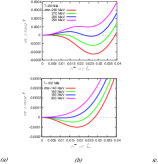
Figure 1: The effective potential, $V[\Sigma_{c}]-V[0]$, with (a) fixed $\mu$ and (b) fixed $T$ as a function of $|\langle{\bar{\psi}}\psi\rangle|$. (c) The contour map of the Landau potential in the $\rho$-$\langle{\bar{\psi}}\psi\rangle$ plane with various chemical potentials for $T=100$ MeV (left) and $T=80$ MeV (right).

We plot $V[\Sigma_{c}]-V[0]$ as a function of $|\langle{\overline{\psi}}\psi\rangle|/\Lambda_{\rm QCD}^{3}$ in Fig. 1(a) at $\mu=0$, 100 and 300 MeV for several values of $T$ and in Fig. 1(b) at $T=80$ and 100 MeV with several values of $\mu$. As seen in Fig. 1(a), a second-order transition occurs in the range $T=$ 100 – 120 MeV in the cases with $\mu=0$ and $\mu=100$ MeV. At $\mu=300$ MeV, however, a first-order transition occurs between $T=75$ MeV and 80 MeV. Similarly, in Fig. 1(b), a first-order transition is seen to occur when the chemical potential is changed between $\mu=280$ MeV and 290 MeV at low temperature ($T=80$ MeV), while the transition is second order at fixed $T=100$ MeV.

In Fig. 1(c), we plot the contour map of the Landau potential given in (18) at several values of $\mu$ with fixed $T$, namely $T=100$ MeV (left) and $T=80$ MeV (right). The vertical axis represents the quark condensate $\langle{\bar{\psi}}\psi\rangle/\Lambda_{\rm QCD}^{3}$, and the horizontal axis represents the quark number density in units of the nuclear saturation density $\rho_{0}$. It is shown that a second-order transition occurs in the left panels of Fig. 1(c). At $\mu=0$, the two minima are positioned symmetrically in the $\rho$-$\langle{\bar{\psi}}\psi\rangle$ plane at $\rho=0$ with finite values of the quark condensate, $\langle{\bar{\psi}}\psi\rangle$. As the chemical potential increases, the two minima approach each other for finite $\rho$, and then fuse continuously to form a single minimum at $\langle{\bar{\psi}}\psi\rangle=0$ and finite $\rho$. At lower $T$ (in the right panels of Fig. 1(c)), a new local minimum appears at $\langle{\bar{\psi}}\psi\rangle=0$ as $\mu$ increases, and three local minima exist in a certain range of $\mu$. These three minima become energetically degenerated at the critical point, and we observe a first-order chiral phase transition. Note that a tri-critical point is located at $(T_{t},\mu_{t})\simeq(97,203)$ MeV, where these three minima merge.

References

- [1] See, for example, Quark-Gluon Plasma 3, ed. R. C. Hwa and X.-N. Wang (World Scientific, Singapore, 2004).
- [2] K.-I. Aoki, M. Bando, T. Kugo, M. G. Mitchard and H. Nakatani, Prog. Theor. Phys. 84 (1990) 683.
- [3] T. Kugo, Dynamical Symmetry Breaking, ed. K. Yamawaki (World Scientific, Singapore, 1992), p.35.
- [4] K. Higashijima, Prog. Theor. Phys. Suppl. 104 (1991) 1.
- [5] H. Fujii and Y. Tsue, Phys. Lett. B357 (1995) 199.
- [6] J. M. Cornwall, R. Jackiw and E. Tomboulis, Phys. Rev. D10 (1974) 2428.
- [7] H. Fujii and M. Ohtani, Phys. Rev. D70 (2004) 014016.
- [8] Y. Hashimoto, Y. Tsue and H. Fujii, Prog. Theor. Phys. 114 (2005) 595.
- [9] S. Sasaki, H. Suganuma and H. Toki, Phys. Lett. B387 (1996) 145.
- [10] N. Goldenfeld, Lectures on Phase Transitions and the Renormalization Group (Addison-Wesley Pub. Co., 1992).