Modeling Bose Einstein Correlations via Elementary Emitting Cells

Abstract

We propose a method of numerical modeling Bose Einstein Correlations by using the notion of Elementary Emitting Cells (EEC). They are intermediary objects containing identical bosons and are supposed to be produced independently during the hadronization process. Only bosons in EEC, which represents a single quantum state here, are subjected to the effects of Bose-Einstein (BE) statistics, which forces them to follow a geometrical distribution. There are no such effects between particles from different EECs. We illustrate our proposition by calculating a representative number of typical distributions and discussing their sensitivity to EECs and their characteristics.

I Introduction

In every high energy collision experiment, a vast number of secondaries (mostly pions) is produced encoding valuable information on the dynamics of the hadronization process. Because of their complexity, such reactions can only be investigated by numerical modeling using specialized codes, Monte Carlo event generators (MCEG) GEN . They all use positively defined probabilities to describe the particle production process. This means that they neglect off-diagonal terms in the corresponding density matrices formally describing such processes. As a result they did not properly implement all the correlations, in particular the quantum mechanical correlations between identical particles (both of Bose-Einstein type for identical bosons (BE) and of Fermi-Dirac type for identical fermions (FD)). The whole collision process is expressed only by the product of single particle distributions. This makes the present MCEG a priori impossible to properly account for results of many experiments (starting from GGLP ), which explicitly show features usually attributed to correlations of this type BEC . To describe such experiments, one has to introduce, in some way, effects of quantum statistics, opening thus a new subject - Bose-Einstein (BEC) or Fermi-Dirac correlations BEC .

This subject already has a long and well documented history BEC but it is still far from complete. Its most specific features one is faced with are the following: In experiments of an exclusive type (measuring all produced secondaries, as in GGLP ) it is possible (at least in principle) to construct the properly symmetrized wave function of all identical pions and thus account for our inability to determine which particle is emitted from which position in the source. In the simplest approach using a plane waves representation of particles, a such wave function for $n_{\pi}$-pion state, has the form zajc :

$$\Psi_{\left\{p\right\}}(\left\{x\right\};\left\{r\right\})=\frac{1}{\sqrt{n_{\pi}!}}\cdot\sum_{\sigma}\exp\left[-i\sum_{j=1}^{n_{\pi}}p_{j}\,r_{\sigma(j)}\right]$$ (1)

($\sigma(j)$ denotes the $j^{th}$ element of permutation of the sequence $\{1,2,...,n_{\pi}\}$ and we sum over all $n_{\pi}!$ permutations in this sequence, including the identity permutation). Points of detection, $x$’s, will vanish when calculating probabilities, but points of production of secondaries, $r$’s, will remain. Because experiments measure only momenta of particles, one must integrate over $\{r_{j}\}$ using some multiparticle spatio-temporal distribution function, $\rho(\{r_{j}\})$. This is usually assumed to be factorizable, i.e., expressed by the product of independent single particle distributions, $\rho(\{r_{j}\})=\prod_{j}\rho(r_{j})$ zajc . Assuming further a totally chaotic hadronizing source one gets the probability of the $n_{\pi}$-pion state in the form of permanent of the matrix $||\Phi_{ij}||$,

$$\mathcal{P}_{1,..,n_{\pi}}\!\!\! = \!\!\!\frac{1}{n_{\pi}!}\sum_{\sigma}\prod_{j}\Phi_{j,\sigma(j)}=perm\,||\Phi_{ij}||=$$ (5)

$$\equiv \frac{1}{n_{\pi}!}\begin{tabular}[]{||cccccc||}&$\Phi_{1,1}$&&$\cdots$&&$\Phi_{1,n_{\pi}}$\\ &$\vdots$&&$\Phi_{j,j}$&&$\vdots$\\ &$\Phi_{n_{\pi},1}$&&$\cdots$&&$\Phi_{n_{\pi},n_{\pi}}$\\ \end{tabular}\,,$$

with

$$\Phi_{ij}=\int e^{iq_{ij}r}\rho(r)d^{4}\{r\},\qquad q_{ij}=p_{i}-p_{j},$$ (6)

(which are all real if $\rho(r)=\rho(-r)$).

However, most of modern experiments are of an inclusive type as one measures effect of BEC on limited samples of secondaries only. The unobserved part of the system acts then as a kind of thermal bath influencing measured samples of data FOOT1 . Also the registered multiplicities are much higher prohibiting calculation of permanents given by eq. (1). The subsystem subjected to further experimental (and theoretical) analysis forms only a (not too well defined) part of the total system with strongly fluctuating characteristics to be averaged during data collection procedure. Because, as we have mentioned, such systems can be described only by numerical modeling, one faces the fundamental question of how to account for BEC in such modeling processes? It must be realized that this is a completely different thing then a simple calculation of the usually considered $n_{\pi}=2$ case, which in the case considered here amounts to a well known expression for the $2-$particle BE correlation function defined as a ratio of a two particle distribution and single particle distributions with $Q=|p_{i}-p_{j}|$ ,

$$C_{2}(Q) = \frac{N_{2}(p_{i},p_{j})}{N_{1}(p_{i})\,N_{1}(p_{j})}=1+\left|\int dr\rho(r)\cdot e^{iQr}\right|^{2}=$$ (7)

$$= 1+\mid\tilde{\rho}(q=Q\cdot R)\mid^{2}$$

($C_{2}\rightarrow 2$ when $Q\rightarrow 0$ and $C_{2}\rightarrow 1$ for large values of $Q$) BEC ; rev ; Z ; Weiner . In fact, in the majority of cases, one is following precisely this route with different functional forms of $\tilde{\rho}(QR)$ and sometimes even with an entirely different form of $C_{2}$ (cf., for example, Kozlov ), but always derived in some analytical way - both for one and three dimensional cases. One is then fitting such correlation functions to appropriate sets of data, aiming to get information on the quantity $R$ (and similar others). The reason for this is that $C_{2}(Q)$ is usually regarded as a (kind of) Fourier transform of the space-time characteristic of the emitting source, $\tilde{\rho}$, therefore providing information on $\rho(r)$ FOOT2 .

It is precisely this fact that makes BEC so interesting, but we shall not follow this route here. Our aim is to provide an algorithm that could cope with BEC from its first steps (to model it) and which could bring this effect to other MCEGs once implemented there. This we shall do by using the notion of Elementary Emitting Cells (EEC) introduced some time ago BSWW . They are some intermediary objects (in fact quantum states) containing identical bosons (henceforth we shall assume them being pions), which are supposed to be produced independently during the hadronization process. Only bosons in EEC are subjected to Bose-Einstein (BE) statistics, which makes them follow a geometrical distribution. There are no such effects between particles from different EECs. Using this idea we propose an algorithm that can be used in any MCEG, which has effects of BEC as one of its basic features. This will be presented on the background of previous attempts to model BEC discussed in zajc ; MP ; MPcells ; Cramer ; ITM . We shall illustrate its action by calculating a representative number of typical distributions and discuss their sensitivity to EECs and their characteristics. In this work no comparison with experimental data is offered, we limit ourselves only to a thorough discussion of our algorithm. It is supposed to be the main building block of any serious MCEG aiming for a real comparison with data and including therefore, for example, also the distribution of energies one is supposed to hadronize or possible flows in the system, i.e., subjects which are out of the scope of this work. In particular it will be most useful in cases where the hadronizing source is well defined (as in $e^{+}e^{-}$ annihilation processes and other elementary processes) or where the number of secondaries is exceptionally large (in high multiplicity events).

For completeness, in the next Section (II) we shall provide a short overview of numerical modelling of BEC proposed so far. This will put our investigation in proper perspective. Section III contains details of the proposed algorithm and examples of results obtained from its simplest version. The last Section contains conclusions and a discussion. Some specific problems connecting with the method proposed are addressed in Appendices A - C.

II History of numerical modeling of BEC

II.1 Imitating BEC with existing MCEGs

Imitating BEC means to use the original outputs of the existing MCEG codes and change them in such way as to reproduce measured $C_{2}(Q)$ (or other experimental characteristics of BEC). Two approaches are used for this. In the first one one introduces some special global weights (i.e., weights built for the whole event) to bias accordingly the original results of MCEG Weights (usually checking whether other observables were not changed too much - otherwise one has to re-run MCEG with new input parameters). This procedure is justified by noticing the following LUND : Let $M=\sum_{\sigma}M_{\sigma}$ be the matrix element describing the production of a hadronic final state of $n$ identical bosons. It consists of $n!$ terms, each corresponding to a particular permutation $\sigma$ of the $n$ identical particles in the final state. In the simulation process of MCEG the interference terms (off-diagonal elements in permanent eq. (5)) are neglected and one gets that the probability to produce such a state is

$$\left|M\right|^{2}_{MCEG}=\sum_{\sigma}\left|M_{\sigma}\right|^{2}\leq|M|^{2}.$$ (8)

To remedy this situation one assumes some weight $\mathcal{W}_{\sigma}$ assigned to each event such that

$$\left|M^{\prime}\right|_{MCEG}^{2}=\sum_{\sigma}\mathcal{W}_{\sigma}\left|M_{\sigma}\right|^{2}.$$ (9)

There is no unique way to choose the weights $\mathcal{W}_{\sigma}$. The only requirements is that one gets good fits to the corresponding $C_{2}$ functions Weights ; LUND . The tacit understanding is that then also $\left|M^{\prime}\right|^{2}_{MCEG}\simeq|M|^{2}$.

In the second approach, one locally modifies (by weighting each pair of particles in a given event) the original output of the MCEG used. This can be done either by modifying its energy momentum spectra Shifts or by changing the resulting charge assignment UWW1 ; UWW2 . In the first case one introduces weight function $f_{BE}(q)$ for pair of particles momenta which are changed, such that

$$\int^{Q}_{0}d\Omega(q)=\int^{Q+\delta Q}_{0}f_{BE}(q)d\Omega(q),$$ (10)

i.e., for $f_{BE}(q)>0$ one has $\delta Q<0$. In this way the energy-momentum imbalance that results from such a procedure is properly accounted for and number of particles, $N=\int d\Omega$, is conserved Shifts . In the second case UWW1 ; UWW2 the original spatio-temporal and energy-momentum structure of the original event is preserved, but often spurious unlike particle correlations occur Unlike . What must be stressed is that this approach, contrary to the previous one, always works on the level of a single event. It is therefore more suitable as an additional tool (sometimes called afterburner) to be used together with the known MCEGs.

It must be stressed that all these methods modify original physics underlying MCEGs in an essentially unknown way FOOT4 . Using them one assumes therefore that changes incurred are small and irrelevant. We shall proceed now to attempts to simulate BEC by which we understand a situation in which the algorithm introducing effects of quantum statistics involves all produced particles zajc ; MP ; Cramer ; ITM .

II.2 Attempts to simulate BEC numerically

II.2.1 Metropolis importance sampling method

In zajc the standard Monte Carlo technique due to Metropolis (Metropolis importance sampling method) was used. This is a general method to generate an ensemble of $n$-body configurations according to some prescribed probability density. In zajc this technique was used to modify the directions of momentum vectors of selected particles from a system of $n$ identical particles in order to impose the $n$-particle distributions derived from BE correlation functions. In particular, it was done by changing the momenta of selected particles, $p_{i}\rightarrow p^{\prime}_{i}\in d^{3}N/dp^{3}$, in such way as to maximize the probability of detection of the $n_{\pi}$-multiparticle state, $\mathcal{P}_{1,...,p_{n_{\pi}}}$, i.e. accepting a new configuration with probability $\mathbb{P}=min\{1,P_{new}/P_{old}\}$, where $P_{old}=\mathcal{P}\{1,...,p_{i},...,p_{n_{\pi}}\}$ and $P_{new}=\mathcal{P}\{1,...,p^{\prime}_{i},...,p_{n_{\pi}}\}$. This procedure is then repeated many times until a kind of ”equilibrium” is achieved. As shown in zajc , one was able in this way to generate typical multipion events, which explicitly exhibit all correlations induced by Bose statistics. The most important result for our further consideration is the fact that as a result of the application of this algorithm a number of objects, called speckles in zajc and being clusters of a number of identical pions in phase-space, is formed. It means that in the multidimensional phase space permanent (5) exhibits rich structure of local maxima (attracting particles) and voids (repulsing them), which replaces the original distribution one started from. Actually the only drawback of this method is that symmetrization of clusters with sizes larger than $n_{cluster}\approx 10$ takes a prohibitively long time.

Two points must be stressed when summarizing this symmetrization procedure. The first is that it involves all (identical) secondaries in the event under consideration, some producing specific structure in their distribution in the allowed phase space, namely it is clustering them in some regions of phase space. The second point is that this phenomenon leads immediately to a broadening of the resultant multiplicity distribution (MD): starting from a Poisson MD for a non-symmetrized wave function one ends up after symmetrization with a geometrical (or Bose-Einstein) MD for a single speckle and with Negative Binomial MD NBD for the whole system.

We close this section with the following remark. So far particles were represented, for simplicity, by plane waves. However, this approach leads to some unpleasant effects because it violates the Heisenberg uncertainty relation constraining the simultaneous specification of coordinates and momentum as implied by eq.(7). For example, in the case of sources with strong position-momentum correlations the two-particle correlation function $C_{2}(Q)$ can drop significantly below unity Weiner ; Problems . This method has therefore been generalized in MP , where plane waves have been replaced by wave packets. Both features mentioned above were also observed here. Therefore in MPcells modification simplifying the selection process was proposed. It was argued that it could be limited only to identical particles whose wave functions overlap in phase space, i.e., to particles forming speckles or clusters mentioned above (with the size of this overlap being a new parameter). Notice that such decomposition corresponds to replacing the full permanent in eq. (5) by matrix with a block structure, each block representing one cluster with no correlations between them:

$$\begin{tabular}[]{||cccccc||}&\framebox{$EEC_{1}$}&&$\cdots$&&0\\ &$\vdots$&&$\ddots$&&$\vdots$\\ &0&&$\cdots$&&\framebox{$EEC_{N_{cell}}$}\\ \end{tabular}\,\,\,.$$ (11)

In what follows we shall identify these blocks with EECs mentioned before. However, it should be remembered that cells selected here were so far preselected in $(\Phi,\Theta)$ space only and, by construction, tend to contain particles with similar momenta. This method differs therefore from that we are going to describe now in which EECs are created dynamically without any restriction Cramer .

II.2.2 The acceptance-rejection method

The acceptance-rejection method used in Cramer is the well known ”hit-or-miss” technique of generating a set of random numbers according to a prescribed distribution, here given by an expression describing the collapse of a multiparticle wave function into a properly symmetrized state represented by eq.(5), as required by Bose quantum statistics. In contrast to that discussed above this method

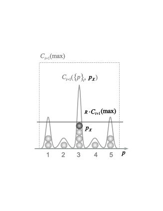
Figure 1: Schematic example of acceptance-rejection algorithm proposed in Cramer at work; $C_{i+1}({\rm max})=(i+1)!$ and $R\in[0,1]$ is random number. For $i$ particles already present with $p_{i=1}$ fixed (gray circles, here $i=9$) one calculates $C_{i+1}(\{p_{1,\dots,i}\},p_{x}=p_{i+1})$ and selects a random number $R$. For the situation shown here (with schematic form of $C(p_{x})$ as example) a new particle can only be added to ”cells” $1$, $3$ and $5$ but not to $2$ and $4$.

is sequential because the $n$ multiparticle event is constructed by adding the $k^{th}$ particle to the $(k-1)$ particles already selected, until $k=n$ is reached. This is done in the following way. One starts with empty phase space and inserts in it the first particle with momentum chosen according to some distribution (for example, the one which is supposed to reproduce single particle spectra). The presence of the first particle causes that a second particle must be added according to the $2$-particle distribution function, which for identical bosons is given by the $2$-particle correlation function $C_{2}\propto P_{1,2}$ with momentum of the first particle fixed and momentum of the second particle to be selected. Because $C_{2}(Q=p_{1}-p_{2})$ has a maximum at $Q=0$, the second particle will tend to be located near the first one in phase space but a priori it can take any position in it. Addition of a third particle must be now performed according to $C_{3}\propto P_{1,2,3}$ (with momenta $p_{1}$ and $p_{2}$ already fixed and only $p_{3}$ being selected), which again has bumpy structure, especially when particles $1$ and $2$ are located far from each other. Therefore the third particle will most probably locate itself near one of the already selected particles but a priori it can take any position in phase space. If, by chance, it will be far away from both particles $1$ and $2$, it will become for future particles a new point of attraction and seed of the new bump. Notice that if, say $k$ particles occupy the same region of phase space, the strength of the bump they form, which attracts other particles, increases $k!$ times. This process, schematically illustrated in Fig. 1, continues until all particles are used (their number can be either preselected, in which case the initial energy will vary, or can result from the procedure itself when initial energy is fixed).

To summarize: this procedure leads again to some specific nonuniform distribution of particles in the allowed phase space with some cell-like structures (bumps) showing up. It results from the fact that regions with some particles inside them already present will have a bigger chance to attract a new particle. Unfortunately, this sequential procedure is even more time consuming than the previous one and therefore rather unpractical.

II.2.3 Information Theory approach

The only workable example of MCEG with features of Bose-Einstein statistics built in from the very beginning has been proposed in ITM . The known total energy $E_{tot}$ has there been distributed among a given (mean) number of secondaries, $\bar{n}=\bar{n}_{+}+\bar{n}_{-}+\bar{n}_{0}$ (where $\bar{n}_{+}=\bar{n}_{-}$), with limited transverse momentum parameterized by the mean value $\langle p_{T}\rangle$, and it was done in such way as to reproduce data on both single particle distributions and those for BEC as well. To this end Information Theory (IT) method was used to obtain the most probable (and least biased) formula for rapidity distributions, $dN/dy$, and multiplicity distributions $P(n)$. It resembles the usual grand canonical distribution but is more general than that because the ”temperature” $T$ and ”chemical potential” $\mu$ occurring there are now two lagrange multipliers obtained by solving the corresponding energy and particle conservation constraints. To also get $C_{2}(Q)$ it turned out that it is enough to additionally divide the available rapidity space into cells of fixed size $\delta y$ each and assumption that each cell can contain only identical particles (i.e., pions of the same charge in this case). It is remarkable that, in addition to reproducing all single-particle characteristics of the collision as well as backward-forward correlations, with this step one gets at the same time also multiplicity distributions $P(n)$ in Negative Binomial (NB) form FOOT5 , the proper structure of the two particle BEC function $C_{2}(Q)$ and intermittency signal FOOT6 . The distinctive feature of this method is that it deals only with measured momenta of produced secondaries, there is no trace on unmeasured spatio-temporal structure present in other methods. If one now wants to somehow deduce this information one has to treat $C_{2}(Q)$ in the same way one is treating all experimental results on BEC (i.e., in fact one has to assume that it is a kind of Fourier transform of the hadronizing source $\rho(r)$ and perform its routine analysis as in rev ; FOOT2 ; WeinerC ).

The most important result of ITM for us is demonstration that the decisive factor leading to proper structure of the correlation function $C_{2}(Q)$ was bunching property in the rapidity space introduced there.

II.3 Quantum optical analogy

Let us therefore concentrate for a moment on this bunching feature of bosons introduced in ITM . At first let us remind ourselves that it has been noticed and discussed already many times Zal ; Pur ; GN ; MPcells and was regarded as manifestation of quantum statistics FOOT6a . It is especially widely discussed and used in quantum optics OPTICS but it was also employed to describe some aspects of the multiparticle production processes BIYA ; QS ; BSWW . This is because $C_{2}$ can be also regarded as some measure of correlation of fluctuations. One uses here the fact that

$$\langle n_{1}n_{2}\rangle = \langle n_{1}\rangle\langle n_{2}\rangle+\langle\left(n_{1}-\langle n_{1}\rangle\right)\left(n_{2}-\langle n_{2}\rangle\right)\rangle$$ (12)

$$= \langle n_{1}\rangle\langle n_{2}\rangle+\rho\sigma(n_{1})\sigma(n_{2})$$

(where $\sigma(n)$ is dispersion of the multiplicity distribution $P(n)$ and $\rho$ is the correlation coefficient depending on the type of particles produced: $\rho=+1,-1,0$ for bosons, fermions and Boltzmann statistics, respectively). It means therefore that one can write the two-particle correlation function (7) in terms of the above covariances (12) stressing therefore its stochastic character UWW1 ; UWW2 ; F :

$$C_{2}(Q) = \frac{\langle n_{i}\left(p_{i}\right)\left[n_{j}\left(p_{j}\right)-\delta_{ij}\right]\rangle}{\langle n_{i}\left(p_{i}\right)\rangle\langle n_{j}\left(p_{j}\right)\rangle}=$$ (13)

$$= 1+\rho\frac{\sigma\left(n_{i}\right)}{\langle n_{i}\left(p_{i}\right)\rangle}\frac{\sigma\left(n_{j}\right)}{\langle n_{j}\left(p_{j}\right)\rangle}-\frac{\delta_{ij}}{\langle n_{i}\left(p_{i}\right)\rangle}.$$

Notice that for geometrical (Bose-Einstein) multiplicity distribution $\sigma^{2}\left(n_{i}\right)=\langle n_{i}\left(p_{i}\right)\left[n_{i}\left(p_{i}\right)-1\right]\rangle$ (corresponding to bosons, $\rho=1$) one gets, for $i=j$, $C_{2}(Q=0)=2$, i.e., its maximal allowed value. This bunching property has already been used in our previous proposition of MCEG of the ”afterburner” type UWW1 ; UWW2 mentioned in Sec. II.1, it was realized in the form of EECs introduced in BSWW . Essentially the same idea will be the cornerstone of our algorithm, which we shall now present. Identical pions will be assumed to be subjected to BEC only when inside EEC, those from different EECs are totally independent (this can be also expressed using notation chaotic and coherent, see Appendix A).

III Modeling Bose Einstein Correlations via Elementary Emitting Cells - our algorithm

III.1 Introduction

The lesson learned from the approaches presented in Sec. II is that construction of the proper quantum multiparticle bosonic state can be performed $(i)$ either by symmetrization of the corresponding wave function constructed for all produced particles zajc ; Cramer ; MP ; MPcells or $(ii)$ by following quantum statistical arguments formulated in Zal ; Pur ; GN and directly bunching produced identical secondaries with (almost) the same energy in phase space to form EECs BSWW ; ITM ; MPcells . So far, the fact that the distribution obtained this way is of NBD type was only shown in zajc . Nevertheless the emergence of bunching (both in zajc and Cramer ) is convincing and makes it an essential characteristic of the bosonic character of produced secondaries one has to account for. This will be our main assumption in what follows.

We have decided to model the effects of proper symmetrization of a multiparticle state by assuring that identical particles are produced in bunches with geometrical distribution of particles. To get such a distribution one has to choose particles sequentially with some prescribed probability $\mathcal{P}$ until first failure. If this failure happens for the $(N+1)^{th}$ trial one gets immediately that

$$P(N)=(1-\mathcal{P})\mathcal{P}^{N}\quad{\rm with}\quad\langle N\rangle=\frac{\mathcal{P}}{1-\mathcal{P}}.$$ (14)

Notice that for $\mathcal{P}$ defined as

$$\mathcal{P}=\mathcal{P}_{0}\cdot\exp\left(-\frac{E_{i}}{T}\right)$$ (15)

(and only then) one gets the usual form of the Bose-Einstein distribution for the $i^{th}$ EEC:

$$\langle N(E_{i})\rangle\equiv\frac{1}{\mathcal{P}_{0}^{-1}e^{E_{i}/T}-1}.$$ (16)

Because, according to eq. (15) $\mathcal{P}_{0}$ controls the maximal number of particles which can be allocated in a given EEC, one can formally introduce a kind of ”chemical potential” (as in ITM ) defined as $\mu=T\ln\mathcal{P}_{0}$ and get FOOT8

$$\langle N(E_{i})\rangle=\frac{1}{e^{\frac{E_{i}-\mu}{T}}-1}.$$ (17)

Such a choice of $\mathcal{P}$ is therefore very crucial in the process of further modeling BEC and is thus the cornerstone of our algorithm.

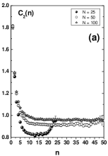
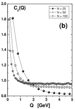
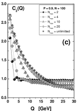
Figure 2: Example of $C_{2}$ occurring for a pionic lattice in (one-dimensional) momentum space: $(a)$ $C_{2}(n)$ as function of number of particles in a given cell for different $N$; $(b)$ $C_{2}(Q)$ as function of $Q$ (in both cases $\mathcal{P}=0.5$). In $(c)$ $C_{2}(Q)$ as function of $Q$ defined by eq. (18) for artificially limited cell occupancy, $i<n_{max}$ (now $\mathcal{P}=0.9$).

Let us now demonstrate this procedure on a simple example of a one-dimensional pionic lattice model UWW2 . The pions located in the sites of the lattice (which prevents identical pions to be found at the same point of phase-space) are endowed with charges in such way that after selecting the charge of the first pion, one assigns the same charge to the consecutive neighboring pions with probability $\mathcal{P}$ until first failure. After failure one assigns (again randomly chosen) charge to the next pion in line and continues this procedure until all pions are used. In this way a number of cells is formed with particles in them distributed by construction (cf. eq. 14) and FOOT8 ) in geometrical fashion, cf., Fig. 2. In Fig. 2a dependence of $C_{2}$ on the lattice spacing defined by different values of $N$ is presented whereas Fig. 2b presents its dependence on $Q$ defined as

$$Q=\mid p_{i}-p_{j}\mid=\frac{2p_{max}}{N}\cdot\mid i-j\mid=\delta p\cdot n$$ (18)

(where $p\in\left[-p_{max},p_{max}\right]$ with $p_{max}=10$ GeV and $N=100$ denotes the total number of sites in our lattice). Comparing them one can deduce that the width of the correlation function, $\sigma(C_{2})$, is roughly proportional to the product of the average number of particles in the cell, $\langle N_{part}\rangle$, and the average distance $\langle\delta p\rangle$ between these particle on the lattice, $\sigma(C_{2})\propto\langle N_{part}\rangle\cdot\langle\delta p\rangle$. Because the average distance between particles on the lattice is fixed by the (constant) lattice spacing, the width of the correlation function depends only on the mean cell occupancy, $\langle N_{part}\rangle$, which is directly related to the probability $\mathcal{P}$ (cf. eq.(16)) and for constant $\mathcal{P}$ all widths of $C_{2}(n)$ in Fig. 2a are the same. Finally, in Fig. 2c the correlation function $C_{2}(Q)$ is shown for different limits $N_{max}$ imposed on the maximal allowed cell occupancy ($i<N_{max}$) (for $\mathcal{P}=0.9$ to assure large occupancy of EECs). Notice that both the value of the intercept parameter, $\lambda=C_{2}(Q=0)-1$, and the width of the correlation function $C_{2}$ depend on the maximally allowed number of pions in one cell, $N_{max}$.

III.2 Implementation

This experience prompted us to propose that BEC should be introduced into the modeling procedure of multiparticle production processes as early as possible, ideally at the very first stage of the selection procedure. It means that one must devise some procedure how to divide a given amount of energy $W$ into produced bosonic particles, assumed to be pions of charges: $(+,-,0)$, without any a priori assumption on what concerns their multiplicities other then $n^{(+)}=n^{(-)}$ but with effects of quantum statistics accounted for. Among procedures mentioned above only that in Sect. II.2.2 Cramer satisfies this demand, however, because it always involves all produced particles, it very quickly becomes impossible to follow because of CPU time demand. On the other hand, results of zajc ; Cramer show explicitly that quantum statistics leads to bunching particles in phase space. Such bunching was therefore assumed in ITM ; MP ; MPcells and in ITM , for the first time, the geometrical distribution form of particles in bunches was used FOOT5 .

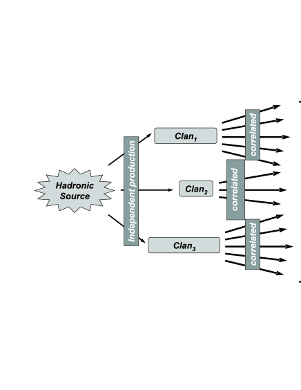
Figure 3: Schematic view of Quantum Clan Model (QCM).

We shall assume therefore that particles are produced according to a mechanism which can be regarded as a quantum version of the clan model (CM) introduced in NBD to explain the fact that apparently all multiparticle production processes result in the NB form of resulting multiplicity distributions $P(N)$; we call it therefore the Quantum Clan Model (QCM), cf. Fig. 3. In CM model (distinguishable) particles are supposed to be produced in clans, which were supposed to be formed independently (and therefore distributed in Poisson fashion), with particles in clans following a logarithmic distribution. Convolution of these two results in the NB form of $P(N)$ ($\mathcal{P}$ denotes the probability of producing a particle),

$$P_{NB}(N)=\left(\begin{tabular}[]{c}$N+k-1$\\ $k-1$\end{tabular}\right)\mathcal{P}^{k}(1-\mathcal{P})^{N}.$$ (19)

In QCM, because of quantum statistics, we must assume that each quantum clan represents a single quantum state and therefore contains only identical particles of (almost) the same energy, which are distributed geometrically BSWW ; Zal ; ITM . Keeping the assumption of independent production of quantum clans, one immediately finds that previous NB multiplicity distribution (19) is now replaced by the so called Pólya-Aeppli (Geometric-Poisson) distribution defined as PA (with $\Theta=(1-\mathcal{P})\langle N\rangle$):

$$P_{PA}(N) \equiv Poisson\bigotimes Geometrical$$ (20)

$$= e^{-\Theta}\mathcal{P}^{N}\sum_{j=1}^{N}\left(\begin{tabular}[]{c}$N-1$\\ $j-1$\end{tabular}\right)\frac{\left[\Theta(1-\mathcal{P})/\mathcal{P}\right]^{j}}{j!},$$ (23)

which was already used in multiparticle phenomenology some time ago FD . It differs from the NB only at small multiplicities. Otherwise it is essentially the same.

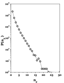
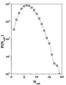
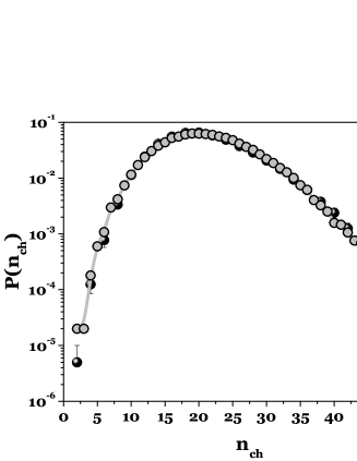
Figure 4: Examples of distribution of particles in a given EEC (upper left panel), distribution of EECs (upper right panel) and total charged particle distribution resulted from the convolution of distributions shown in the first two panels (lower panel, open circles and solid curve, see text for details). Notice that, with this choice of parameters, one can reproduce exactly the experimental data for $e^{-}e^{+}$ annihilations taken at the same energy DELPHI (black circles).

To implement numerically the QCM we proceed in the following way.

$(i)$ A pion of randomly chosen charge is selected with energy $E_{1}=E_{EEC}$ following some assumed distribution $f(E)$. The form of this distribution is dictated by physics of the model used to describe the production process which we would like to follow (much the same as in Cramer ). It has no influence on the bosonization (other then emerging from conservation laws), on the other hand it strongly affects the final form of multiparticle distributions obtained (by changing effective distributions of EECs). This pion is therefore supposed to be the seed for the first EEC.

$(ii)$ The other pions of the same charge are than added, one after another, using probability $\mathcal{P}$ as given by eq. (15). This is done until the first failure, which marks the end of formation of the first EEC. After that, one starts formation of another EEC by proceeding to point $(i)$ and choosing from $f(E)$ another energy $E_{EEC}$ of another pion of randomly chosen charge, which forms the seed of the second EEC. The whole procedure is repeated until all available energy $M$ is used up.

$(iii)$ Once accepted, each of the selected pions forming the first EEC is endowed with energy $E_{i}$ ($i\geq 2$), which is selected from some distribution $G(E_{i})$ centered on the energy of the first pion forming the seed of this EEC, $E_{EEC}$. The sense of the function $G(E_{i})$ is that it reflects the fact that the requirement that all particles belonging to a given EEC must be in the same energy state, in which case one expects that $G(E_{i})\sim\delta\left(E_{EEC}-E_{i}\right)$, means that their energies can differ only by an amount corresponding to the width of the spectral line mentioned in Pur . We shall then use $G(E)$ either in the form of delta function mentioned above or parameterize it by a Gaussian,

$$G(E_{i})=\frac{1}{\sqrt{2\pi}\sigma}\exp\left[-\frac{\left(E_{EEC}-E_{i}\right)^{2}}{2\sigma^{2}}\right].$$ (24)

In the thermal-like model for $f(E)$ used here, there is a natural length scale given by the temperature $T$ and it is therefore natural to choose $\sigma$ as being proportional to it, we shall therefore take $\sigma=\sigma_{0}T$ (for the possible physical meaning of $\sigma$ see Appendix B).

Table 1: The mean total multiplicities and their dispersions ($\langle N\rangle$ and $\sigma_{N}$), the mean total multiplicities of EECs and their dispersions ($\langle N_{cell}\rangle$ and $\sigma_{N_{cell}}$) and mean multiplicities and dispersions in EEC ($\langle N_{part}\rangle$ and $~{}\sigma_{N_{part}}~{}$) calculated for some selected choices of parameters $\mathcal{P}_{0}$ and $T$ (upper part) and for different initial energies ($W(i)=0.5W$, $W(ii)=W=91.2$ GeV and $W(iii)=2W$ - lower part). All results are for $\sigma_{0}=0.0$ except the middle part, which was obtained for $\sigma_{0}=0.3$ for comparison.

$\mathcal{P}_{0}$	$T$	$~{}\langle N\rangle~{}$	$~{}\sigma_{N}$	$~{}\langle N_{cell}\rangle~{}$	$~{}\sigma_{N_{cell}}$	$~{}\langle N_{part}\rangle~{}$	$~{}\sigma_{N_{part}}$
$0.9$		41.39	12.87	18.21	3.24	2.27	2.61
$0.7$	$3.5$	33.81	8.28	20.58	3.73	1.64	1.28
$0.5$		30.34	6.63	22.41	4.11	1.35	0.78
$0.3$		28.22	5.69	24.01	4.44	1.17	0.48
	$1.5$	82.68	15.29	39.85	4.66	2.07	2.13
$0.9$	$3.5$	41.39	12.87	18.21	3.24	2.27	2.61
	$5.5$	27.99	11.13	12.03	2.64	2.32	2.78
0.7	3.5	32.05	7.12	19.54	3.47	1.63	1.27
$W$	$T$	$~{}\langle N\rangle~{}$	$~{}\sigma_{N}$	$~{}\langle N_{cell}\rangle~{}$	$~{}\sigma_{N_{cell}}$	$~{}\langle N_{part}\rangle~{}$	$~{}\sigma_{N_{part}}$
	$\mathcal{P}_{0}$
$(i)$	$3.5$	21.22	9.08	9.49	2.29	2.24	2.56
$(ii)$	$0.9$	41.39	12.87	18.21	3.24	2.27	2.61
$(iii)$		81.70	18.27	35.62	4.58	2.29	2.65

In this work we shall use the function $f(E)$ in the form of a Boltzmann distribution,

$$f(E)=\exp\left(-\frac{E}{T}\right),$$ (25)

corresponding to a kind of thermal-like model with temperature $T$ being the main parameter. In this case the parameter $\mathcal{P}_{0}$, governing the number of particles in EECs, plays role of the chemical potential. As expected, one gets then EECs distributed according to a Poisson distribution, each EEC containing particles of the same charge only, which are distributed according to Bose-Einstein (or geometrical) distribution, also the shape of charged particle multiplicity distributions comes out as expected, see Fig. 4. It was obtained for hadronizing energy $W=91.2$ GeV using $T=3.5$ GeV, $\mathcal{P}_{0}=0.7$ and $\sigma_{0}=0.3$. For the corresponding values of mean multiplicities and their dispersion cf. Table 1 (the middle row).

The $W=91.2$ GeV value of energy will be used throughout the paper (chosen to allow for the only comparison with data we show in Fig. 4). In all examples shown here the number of MC trials was $N_{MC}=50000$ and reference frame used to calculate $C_{2}$ function is composed from $(+-)$ particles whereas $C_{2}$ themselves are calculated for $(--)$ pairs. Table 1 shows the corresponding multiplicities (and their dispersions) of all particles obtained when hadronizing mass $W$ and those for the total number of EECs and particles in them. The bigger $\mathcal{P}_{0}$, the bigger the total multiplicity, smaller the number of EECs and bigger their occupancy. Increase of $T$ decreases the total multiplicity and number of EECs but slightly increases their occupancy. The increase of available energy $W$ results in an increase of all these quantities, except for the cell occupancy, which remains essentially the same.

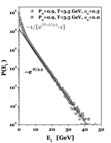
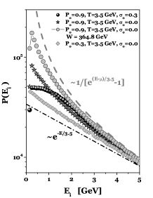
Figure 5: Comparison of energy distributions obtained using zero and nonzero values of $\sigma_{0}$ compared (dashed-line) with the corresponding Bose-Einstein form of energy dependence of occupation number as given by eq. (16). The mass of hadronizing source is $W=91.2$ GeV, except the last curve where it is $4$-fold greater for comparison.

Fig. 5 shows an example of the corresponding energy distributions of produced secondaries. Notice that the effect of bunching (i.e., effect of introducing EECs) is visible only in the limited range of the allowed phase space, concentrated at small energies. In the case considered here, where the allowed range is $(1/2)\cdot(W=91.2)$ GeV, it practically vanishes for $E>7.0$ GeV and after that value the distribution follows the exponential form of $f(E)$ we have started from. This means that BEC increases the multiplicity of event by adding particles with small energies (see also Table 2). Notice that for nonzero $\sigma_{0}$ one gets a displaced maximum for small values of $E$. At large energies results follow the shape of the original $f(E)$ distribution (25) used here. The other important feature is the fact that none of the numerical simulations reproduces the Bose-Einstein form of energy dependence of occupation number, usually used in all analytical estimations and given by eq. (16). This is because of the finiteness of available energy $W$ one can use for hadronization, which results in limited occupancy of EECs and violates conditions used to obtain eq. (16) FOOT8 . Detailed results on the mean number of EECs and charged particles multiplicity in them in different energy bins are presented in Table 2.

Table 2: The mean number of EECs, $N_{cell}$, and charged particles multiplicity in them, $n_{\pi^{-}}$, in different energy bins calculated for $T=3.5$ GeV and two sets of $(\sigma_{0},\mathcal{P}_{0})$.

Bins in $E$	$\sigma_{0}=0.1$; $\mathcal{P}_{0}=0.9$		$\sigma_{0}=0.3$; $\mathcal{P}_{0}=0.7$
(GeV)
	$N_{cell}~{}~{}$	$n_{\pi^{-}}$	$N_{cell}$	$n_{\pi^{-}}$
$0.0-0.5$	0.58	2.62	0.63	1.2
$0.5-1.0$	0.72	3.00	0.79	1.60
$1.0-2.0$	1.16	2.98	1.26	2.62
$2.0-3.0$	0.87	1.58	0.95	1.70
$3.0-5.0$	1.15	1.64	1.25	1.76
$5.0-7.0$	0.65	0.77	0.71	0.83
$>7.0$	0.84	0.89	0.92	0.97

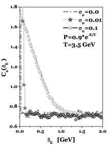
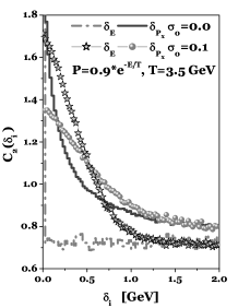
Figure 6: Illustration of importance of spreading in energy. Left panel: $C_{2}(\delta_{E})$ case with of $\sigma_{0}=0.0$, $0.01$ and $0.1$. For $\sigma_{0}=0$ the maximum of $C_{2}$ is divergent (all points are in the first bin). Right panel: $C_{2}(\delta_{E,p_{x}})$ cases with $\sigma_{0}=0.0$ or $\sigma_{0}=0.1$. Notice that $C_{2}(\delta_{p_{x}})$ (calculated for momenta distributed isotropically) has nonzero width even for $\sigma_{0}=0$. Introducing nonzero $\sigma_{0}$ results in further broadening of $C_{2}$.

We now proceed to the correlation functions $C_{2}(\delta_{X}=X_{1}-X_{2})$ and start with distributions in energy, $C_{2}(\delta_{E})$ . In Fig. 6 one observes that when using $\sigma_{0}=0$ (i.e., for strictly $\delta$-like form of $G(E)$) the whole effect is located in the first bin only (this is just computer realization of delta function). Therefore, if nonzero widths of $C_{2}$ are needed, one must use $\sigma_{0}>0$. Notice, however, that this width is not equal to the input $\sigma=\sigma_{0}T$ used because the difference of two variables, each following the same Gaussian distribution, is again Gaussian but with twice $\sigma^{2}$, therefore the final distribution should be $\sim\sqrt{2}$ broader, which is roughly the case shown in Fig. 6 (where $\sigma=0.35$ GeV was used as input in (24) whereas the width which can be read off from the obtained shape of $C_{2}$ is equal to $0.45$ GeV).

We must stop for a moment to comment the fact that, in all figures presenting $C_{2}(\delta_{X})$ shown here, their values are significantly smaller than unity for large values of $\delta_{X}$. This is not an artifact of our algorithm, but results from the method of presentation of our output. We want to keep the same number of pairs both in the real event and in the reference one (which, in our work, is always built from pairs of opposite charges). Technically it means that one has to conserve the area under each curve for $C_{2}(\delta_{X})$. Actually this effect is also known in all other approaches to BEC and is usually corrected by arbitrarily shifting $C_{2}$ in such way that it equals unity for some large value of the argument (in practice set to be equal $1$ GeV) Weights . We shall not do this here, but this fact must be remembered when looking at our results.

In Fig. 6 $C_{2}(\delta_{E})$ is compared with $C_{2}(\delta_{p_{x}})$ calculated assuming an isotropic distribution of momenta of particles in a given EEC, $\vec{p}$. The freedom presented in the choice of directions of momenta results in a nonzero width of the otherwise $\delta$-like structure of $C_{2}(\delta_{E})$ for $\sigma_{0}=0$. It then further broadens when one allows for some nonzero width $\sigma_{0}$. This means that it can be used as an additional parameter when comparison with data would be attempted (provided its physical meaning will be made clear, see, for example, the discussion in Appendix B and fractality ).

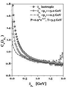
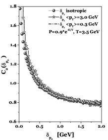
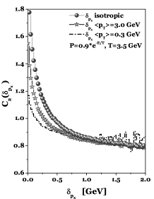
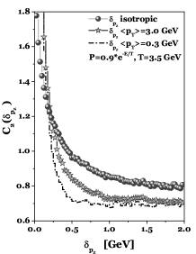
Figure 7: Comparison of two different ways of choosing momenta of particles occupying given EEC ($|\vec{p}|$ is always fixed) for $\delta_{p_{x}}$ (left panels) and $\delta_{p_{z}}$ (right panels). Upper panels: the $(+,-)$ sign of $p_{L}$ was chosen randomly for every particle without referring to EEC it belongs to. Lower panels: it was chosen randomly for EECs and kept the same for all particles in it. In all cases three choices of $p_{T}$ is shown: unlimited (isotropic) and with limits imposed by two different values of $\langle p_{T}\rangle$ when sampling $p_{T}$ from exponential distribution; in all cases $\sigma_{0}=0$ .

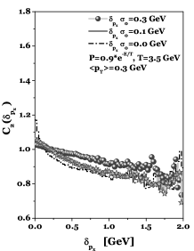
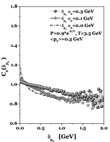
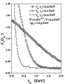
Figure 8: The same as in Fig. 7 but for choice of $p_{T}$ restricted by $\langle p_{T}\rangle=0.3$ GeV and for different values of $\sigma_{0}=0.0$, $0.1$ and $0.3$.

If one wants to further continue with $C_{2}\left(\delta_{p_{x,y,z}}\right)$, some additional input (new parameter(s)) is necessary, which has to be justified. We shall not discuss this point in detail, as it would bring us outside the main scope of this paper. Instead, we limit ourselves to showing in Fig. 7 the results of some more refined choices of directions of momenta. All results are for $\sigma_{0}=0$, introduction of nonzero $\sigma_{0}$ will change them accordingly in the manner presented in Fig. 6. They were obtained by choosing first values of transverse momenta, $p_{T}=|\vec{p}_{T}|$, by selecting them from some exponential distribution constrained only by the assumed mean value, $\langle p_{T}\rangle$, which serves therefore as new parameter. This corresponds to selection of polar angles from the band centered on $\Theta_{mean}=\arctan\left(\langle p_{T}\rangle/p_{L}^{(max)}\right)$), the corresponding axial angles were chosen uniformly from the $[0,2\pi]$ range. In this way, one gets components $p_{x}$ and $p_{y}$ and longitudinal component $p_{z}=p_{L}=\pm\sqrt{p^{2}-p^{2}_{T}}$. Two natural situations are considered here: $(i)$ - the maximally isotropic case (the $p_{L}$ of every consecutive particle, irrespectively of the EEC they belong to, is randomly assigned the sign $(\pm)$) and $(ii)$ - the case in which bunching in energies is preserved also on the level of momenta (all particles in a given EEC have $p_{L}$ in the same hemisphere). All other choices should interpolate between these two.

Two characteristic features seen in Fig. 7 should be noticed: $(i)$ one observes narrowing of $C_{2}(\delta_{p_{x}})$ (i.e., transverse) distributions with tightening the allowed $p_{T}$ region (i.e., when proceeding from fully isotropic distributions to those restricted by assumed $\langle p_{T}\rangle$ with diminishing values of $\langle p_{T}\rangle$), this effect is essentially independent of the way the signs of $p_{z}$ components are chosen. $(ii)$ $C_{2}(\delta_{p_{z}})$ shows different behavior depending on which choice of signs is followed: it shows no dependence on $\langle p_{T}\rangle$ for the choice $(i)$ above whereas for the choice $(ii)$ a difference shows up only for $\delta_{p_{z}}>0.2$ GeV. The situation changes dramatically when one allows for smearing of energy in the EEC, i.e., for $\sigma_{0}>0$, see Fig. 8. This means introducing a new parameter, to which our results are most sensitive but which is still not well understood (see, for example Appendix B).

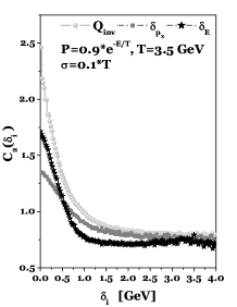
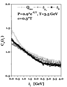
Figure 9: Comparison of $C_{2}(\delta_{i}=\delta_{E,p_{x}})$ as presented in Fig. 6 for $\sigma_{0}=0.1$ with $C_{2}(\delta_{i}=Q_{inv})$ for the same parameters (left panel). Notice that maximum of $C_{2}(Q_{inv}=0)>2$ and to get it below this value one has to increase $\sigma_{0}$ (see right panel with $\sigma_{0}=0.3$).

In Fig. 9 results for $C_{2}(\delta_{E})$ and $C_{2}(\delta_{p_{x}})$ are compared with those for $C_{2}(Q_{inv})$, where $Q^{2}_{inv}=-\left(p_{1}-p_{2}\right)^{2}$ with $p_{1,2}$ being $4$-momenta of particles $1$ and $2$ (it is relativistically invariant variable , such that $Q_{inv}^{2}=0$ implies for massive particles that $\vec{p}_{1}=\vec{p}_{2}$ and BEC has its maximum there). Notice the peaked shape of $C_{2}(Q_{inv})$ and the fact that $C_{2}(Q_{inv}=0)>2$ here. As shown in Q2 both features are mostly due to the specific kinematics of the $Q_{inv}$ variable (because of which it collects in the first bin contributions from the whole range of momenta provided only that they are near enough to each other). The point is that in case of $Q_{inv}$ variable smearing $\sigma$ in energy $E$ and smearing in momentum $p$ are not independent and therefore they do not sum up (as is the case for independent variables) but rather they tend to cancel. In fact, their global effect is of the order of $\sigma\cdot(\sqrt{p^{2}+m^{2}}-p)$ which tends to zero for large momenta and never exceeds $\sigma\cdot m$, where $m$ is pion mass. In other words, smearing in $Q_{inv}$ is considerably smaller then that in energy and momentum. Therefore there is a natural tendency of increasing occupancy of the lowest bins in $\delta_{i}=Q_{inv}$ in comparison to $\delta_{E}$ or $\delta_{p_{x}}$.

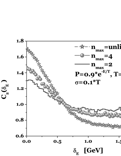
Figure 10: Comparison of $C_{2}(\delta E)$ for different maximally allowed sizes of EEC given by maximal number of particles $n_{max}$ they can have. Notice difference from the similar results obtained for pionic lattice and presented in Fig. 2c. It is caused by the fact that here distance between particles is not limited by the fixed spacing of the lattice as before.

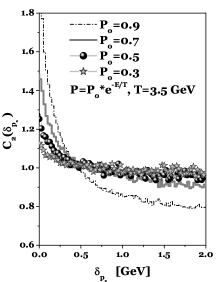
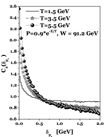
Figure 11: Upper panels: sensitivity of $C_{2}(\delta_{p_{x}})$ to different choices of EECs exemplifying by different sets of parameters used. Lower panel: the same but for different energies $W$ and fixed size of EEC (as indicated, in all cases $\sigma_{0}=0$ and isotropic source was considered). The corresponding values of mean multiplicities, their dispersion as well as the mean number of EECs and their mean occupancies are listed in Table 1.

Let us now stress the most specific feature of our algorithm: it always produces BEC of the highest possible order $n$ (for which $C_{2}(\delta_{E}=0)=n!$). This order is dictated by the the number of particles in the most populated EEC, which in turn depends strongly on location of a given EEC in phase space, see Table 2. It will significantly influence both the strength (as given by $C_{2}(\delta=0)$) and shape of the BEC effect, cf., Fig. 10. In it we show what happens when the maximal number of particles in each EEC is artificially limited so as not to exceed some imposed maximal value equal to $n_{max}$. Notice that this requirement also affects the resulting number of EECs (the smaller population of EECs the more of them must be present). It is clear that this effect will be strongest in events with very high multiplicities recorded (cf. LargeN for references to projects of the respective experiments). The sensitivity of our algorithm to $n_{max}$’s presented in Fig. 10 (for $C_{2}(\delta_{p_{x}})$ the changes are qualitatively the same for all choices of momenta presented here) makes it an ideal tool for numerical investigations of BEC also for particles satisfying statistics different than BE (for example, the so called parastatistics parabosons ).

We close this Section showing how sensitive are $C_{2}(\delta_{i})$ to different choices of EECs represented by different values of parameters $\mathcal{P}_{0}$ and $T$ and to different masses $W$ of hadronizing source, cf. Fig. 11 and Table 1 (this is done again for $\sigma_{0}=0$ and using isotropic distributions of directions of momenta. Any changes in them, as discussed before, would then change these results accordingly in the way demonstrated in Figs. 6, 8 and 7). The most characteristic feature is the observed growth of $C_{2}(\delta_{i}=0)$ (i.e., the grow of the so called ”parameter of chaoticity” $\lambda=C_{2}(\delta_{i}=0)-1$ ) with diminishing number of EECs, $\langle N_{cell}\rangle$. Actually, this result was behind the original introduction of the notion of EECs in describing the BEC effect done in BSWW where the number of EECs is tightly connected with the parameter $k$ in the NB multiparticle distributions used to fit data. Interesting feature of this approach, shared by our picture as well, is that, as shown in BSWW , it explains in a natural way the dependence of $\lambda$ on $dN/dy$ and on the atomic number of projectiles $A$ FOOThalo . In Appendix C we discuss changes in $C_{2}(\delta_{i})$ introduced when correcting for the inevitable energy-momentum and charge imbalances induced by our algorithm.

III.3 Discussion

Let us recapitulate the physical picture we are proposing. Its basic object is an EEC, a quantum state containing a number of identical secondaries of the same, or nearly the same energies. These secondaries are assumed to satisfy the BE statistics which is imposed by demanding that they follow geometric distribution. As a result the correlation functions $C_{2}(\delta_{X})$ that follow are very sensitive to the characteristics of the EEC, for example the width of $C_{2}(\delta_{X})$ is proportional to the allowed energy spread in EEC, $\sigma$. It is best seen on the example of $C_{2}(\delta_{E})$, cf. Fig. 6. Interestingly enough, when all particles in the EEC have the same energy, $C_{2}(\delta_{E})$, is divergent. On the other hand, in the same situation, correlation functions in momenta have already nonzero widths. This is because the choice $\sigma=0$ does not constraint directions of momenta. The simplest case of isotropically selected directions, represented by $C_{2}(\delta_{p_{x}})$, is shown in Fig. 6. The choice of directions provides therefore additional freedom in modeling $C_{2}(\delta_{p_{x,z}})$. It can be seen in Figs. 7 and 8 where examples of restricting the range of transverse momenta and the choice of longitudinal momenta are displayed. As for the physical meaning of $\sigma>0$, it is tempting to identify it with the temporal characteristic of hadronization process, in fact with the life time of an average EEC.

So far we presented results only for direct pions being produced. To include resonances one would first have to decide whether the BEC should affect them in the same way as particles or whether they affect only the pions resonances decay into. This point surely deserves further discussion, but it would bring us outside the scope of our paper. Therefore we present in Fig. 12 results for $C_{2}$ calculated for $\rho$ mesons (of charges $(+,-,0)$ and mass $m_{\rho}=0.7$ GeV, with zero widths assumed for simplicity) considered to be simple particles subjected to the same procedure of building EEC as that for pions. This is compared with the case where such $\rho$’s subsequently decay into pions.

Figure 12: Comparison of BEC for mesons $\rho$ (with $m_{\rho}=0.7$ GeV) and for pions obtained from their decays. To maximize effect we use the EEC’s for $\rho$’s with fixed energies (i.e., $\sigma_{0}=0$). Both $C_{2}(\delta_{E})$ and $C_{2}(\delta_{p_{x}})$ are presented. Notice that also for $\rho$ correlation function $C_{2}(\delta_{E})$ is concentrated in first bin only.

Notice that whereas the BEC for $\rho$’s is quite strong and not very much different from that for pions only, it hardly survives the process of $\rho$’s decay, especially for the $C_{2}(\delta_{p_{x}})$ case. However, it must be stressed at this point that, so far, our $\rho$’s were treated as spinless particles and that they were assumed to decay into pairs of pions in an isotropic way in their center of mass FOOT12 .

In our algorithm only particles in EEC are subjected to BEC, there are no intercorrelations of the BE type between particles from different EECs (see Appendix A). Such picture seems to be supported by recent data on BEC in $e^{+}e^{-}\rightarrow W^{+}W^{-}$ multi-$W$ boson production which show non existence of inter-$W$ BEC. This result suggest strongly that although spatially located practically on top of each other, nevertheless bosons $W$ act as independent sources of pions in this case eeWW .

We would like to stress here that all restrictions on energies and momenta mentioned above influence first of all the shape of a single EEC in momentum space rather than global characteristic of a given hadronizing source used. It is therefore to a large extent the EEC information on which are encoded in the correlation function $C_{2}$. On the other hand their number depends in the first instance on the characteristics of the hadronizing source encoded in the choice of $f(E)$. Occupancy of EEC, however, depends strongly on $\mathcal{P}_{0}$ and together with $T$ from $f(E)$ change substantially both the multiplicity distributions (in our case from the Poisson-like to Pólya-Aeppli one) and single particle distributions as well (see Figs. 4 and 5).

Figure 13: Example of intermittency signals obtained using our algorithm with $\mathcal{P}_{0}=0.9$, $T=3.5$. Left panel: not corrected for energy-momentum and charge imbalances results for $\sigma_{0}=0$ (black curves) and $\sigma_{0}=0.3$ (grey curves) are compared. Right panel: results for $\sigma_{0}=0$ only with and without corrections (most of the visible effect comes from correcting the energy momentum imbalance). Moments $F_{q}(M)$ are defined as in Intermitency .

It is worth to mention at this point that together with BEC our algorithm introduces also some intermittency signal, much in the way expected already in FOOT6 , see Fig. 13. It depends noticeably on the smearing of EEC in energy and is very sensitive to the energy momentum imbalance corrections (cf., Appendix C) Sarki .

IV Summary and conclusions

To summarize: we argue that proper numerical symmetrization of the multiparticle state of identical particles can be achieved in an economical way (in what concerns computational time) only by bunching them in phase space in such way that (identical) particles in each bunch (called here EEC - elementary emitting cell) have (almost) the same energies and follow a geometrical (Bose-Einstein) distribution. Only particles in EEC experience BEC, those from different cells do not (see Appendix A). We regard this conjecture as emerging in a natural way from previous investigations zajc ; MP ; Cramer ; ITM ; AIP . It is the main result of studies of a properly symmetrized multiparticle wave function of identical secondaries produced in the reaction zajc ; MP ; Cramer . They unravelled that in such state the originally uniformly distributed particles start to bunch zajc ; Cramer , also changing the original poissonian multiplicity distribution to a NB one zajc . The similarity with the clan model NBD leading to QCM proposed here was then immediate. The same conjecture was achieved independently following studies in which one works with number of quanta (particles) without invoking wave functions Zal ; Pur ; GN ; OPTICS ; BIYA ; QS ; F . In the first practical application of the concept of bunching ITM the whole (one dimensional) phase space was divided into such EECs (of equal size in rapidity space) and this simple decision resulted in profound consequences for what concerns the ability to describe different physical distributions. We develop this idea further: our EECs are formed dynamically, they can both overlap each other and be widely separated from each other and their number and multiplicities (i.e., their sizes) of particles in them fluctuate from event to event. This work is then about how to form such EECs and what to do with them.

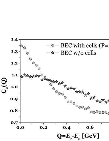
Figure 14: Comparison of $C_{2}$ modelled by using MC event generators with EEC (circles) and without EEC’s but with selecting particles directly from the corresponding Bose-Einstein distribution $\langle N(E_{i})\rangle$ as given in eq. (17) THERMINATOR . In both cases the Boltzmann distribution for classical particles was used as reference event. This fact may be crucial to get apparent increase in case of using directly Bose-Einstein distributions (as in THERMINATOR ). The use of mixed event instead, which will not affect substantially the result obtained using EECs, will most probably kill the other effect.

One can ask whether cells (or proper bunching of identical particles in phase-space, advocated here) are really needed to model quantum Bose statistics or, perhaps, is would be enough just to use the usual Bose-Einstein distributions to this aim. To answer this question let us compare two ways of producing bosonic particles: $(i)$ generating them directly from Bose-Einstein distribution (like $\langle N(E_{i})\rangle$ as given in eq. (17), which is the most simple way advocated on many occasions) and, $(ii)$ generating particles from a Boltzmann distribution and bunching them in an appropriate way in phase-space according to QCM presented here. In the first case, one gets the correct single particle distribution, whereas in the second case one also accounts for multiparticle correlations of quantum statistical origin. The corresponding results are presented in Fig.14. They show that both approaches lead to very different results, which can be understood by realizing that case $(i)$ corresponds to a particular realization of case $(ii)$, namely with only one cell containing the same average number of particles. In fact case $(i)$ shows only some trivial correlations which can be eliminated by a proper choice of the reference distribution. Therefore, we argue that, according to our understanding, the better approach (after correcting additionally for charge and energy-momentum conservations) is that

BEC = cells + geometrical distribution (26)

From its construction it is evident that our algorithm is best suited to study events with large multiplicities (as planned in some experiments LargeN ). The statement (26) also summarizes the only possible way to incorporate our algorithm in MCEG codes: according to our finding it should be done by enforcing particles to be produced in bunches with characteristics of our EECs. In fact, closer inspections on all previous efforts to imitate BEC mentioned in Section II.1 shows that they all implicitly were aiming in similar direction Weights ; LUND ; Shifts ; UWW1 ; UWW2 . The difference was that they were trying to do it a posteriori rather than a priori and that their weighting procedure was aimed more at the spatio-temporal (unknown) characteristics of the hadronizing source than on the true physical principles of BEC.

In this work we have stopped short of a general comparison with data. The reason is that we were using here a most simple statistical model of hadronization in order to illustrate our algorithm. According to it a hadronizing source is assumed to be a single object with some fixed mass $W$ and fixed initial charge, which is the situation encountered only in $e^{+}e^{-}$ annihilation reactions. In all other multiparticle production processes one either encounters $W$ varying from event to event (following some distribution, for example, inelasticity distribution inel ) or there is a number of hadronizing sources with different $W$ in each event (which is the most probable situation in heavy ion collisions). Moreover, the statistical scheme of hadronization employed here means that our hadronizing source does not experience any internal flows and is not subjected to any external force, which would result in some energy-position correlations or specific effects of partial coherence (cf., Kozlov ) and thus additionally influence the $C_{2}$ correlation function. The problem of the possible net charges of such sub-sources was never discussed. All this asks for very specialized study, which goes outside the scope of this paper. What we can only say at this moment is that, when undertaken, such a study would mean the necessity of developing our formalism further in what concerns details of modeling EECs mentioned before. The most probable approach would be to additionally assume that each EEC itself should be described by a properly symmetrized $n_{part}$-particle wave function (where $n_{part}$ is the number of particles in this EEC). Only then would one be able to introduce into the model a characteristic momentum-positions correlations caused by quantum statistics (much in the spirit leading to eq. (1)). The price for following such a procedure is the necessity to also introduce to our description the space-time characteristics of the hadronizing source, which we were not dealing with so far. This would result in the same permanent structure as given by eq. (5), but with much smaller sizes and with explicit dependence on spatio-temporal variables (as in eq. (11)) to be used later when selecting momenta (actually, they would be effectively integrated out in this procedure). However, the noticeable feature is that in our case this procedure would not demand spatio-temporal factorization property of the hadronizing source assumed in (1). When replacing plane waves used there by Coulomb distorted wave functions BCoul (which is common practice nowadays) one could then attempt, in principle, to account for the influence of Coulomb interactions so far neglected here (albeit only on the level of $2$-body interactions). This is, of course, not the only possible generalization and therefore we leave the problem of confrontation with real data for further studies. Finally, let us notice that any serious comparison with data would have to be done including corrections for energy-momentum and total charge imbalances induced by our algorithm, which (as seen in Appendix C) can be quite substantial and not unique.

Let us close by noticing that, although our algorithm was originally intended to model quantum phenomena of BEC only, it is in fact more general. The reason is that the characteristic structure of the $C_{2}$ correlation function associated with specific bunching of identical particles turns out to be quite universal phenomenon also observed in many other, purely classical systems, provided only that they exhibit strong and correlated fluctuations Classical . This means then that our algorithm, albeit with different motivation, could also be applied there. At this point one should also notice an attempt at numerical modeling of another quantum phenomenon, namely Bose-Einstein condensation presented in KR and the possible connection of the above with the physics of networks Net . Finally, we also claim that, because of its sensitivity to maximal occupancy of EECs, out method could easily be modified to be able to study BEC effects for para-bosons parabosons .

Acknowledgements: Partial support by the Ministry of Science and Higher Education (grant 1 P03B 022 30 - OU and GW) is gratefully acknowledged .

Appendix A Some remarks on EEC

We would like to comment in more detail on our proposition that identical bosons should come in EEC and experience effects of BEC there, whereas no such effects should be seen when bosons from different cells are considered. In the language used in Glauber the probability of registration of a coincidence of $n$ bosons in states $j_{1},\dots,j_{n}$ is given by a normalized correlation tensor of rank $2n$,

$$g_{j_{1}\dots j_{n}j_{n+1}\dots j_{2n}}^{(nn)} = \frac{G^{(nn)}_{j_{1}\dots j_{n}j_{n+1}\dots j_{2n}}}{\prod_{i=1}^{2n}\sqrt{G^{(11)}_{j_{i}j_{i}}}},\quad{\rm where}$$ (27)

$$G^{(nm)}_{j_{1}\dots j_{n}j_{n+1}\dots j_{n+m}} = Tr\left\{\rho a^{{\dagger}}_{j_{1}}\dots a^{{\dagger}}_{j_{n}}a_{j_{n+1}}\dots a_{j_{n+m}}\right\}$$

is given in terms of the density matrix operator $\rho$ whereas $a^{{\dagger}}$ and $a$ are, respectively, creation and annihilation operators. If

$$|g^{(nn)}_{j_{1}\dots j_{2n}}|=1\qquad n\leq N$$ (28)

we have coherence of the order $2N$. Experimentally this means that the probability of registering $n$ bosons in coincidence is equal to the product of probabilities to register individual ones. Because of commutation relations for bosons, $\left[a_{k},a_{l}\right]=\left[a_{k}^{{\dagger}},a_{l}^{{\dagger}}\right]=0$ and $\left[a_{k},a_{l}^{{\dagger}}\right]=\delta_{kl}$, one has that $a_{k}^{{\dagger}}a_{l}^{{\dagger}}a_{k}a_{l}=a_{l}^{{\dagger}}a_{k}^{{\dagger}}a_{k}a_{l}=a_{k}^{{\dagger}}a_{l}^{{\dagger}}a_{l}a_{k}=a_{l}^{{\dagger}}a_{k}^{{\dagger}}a_{l}a_{k}=n_{k}n_{l}$ and then from eq. (27) that for two bosons from different states

$$g^{(22)}_{k_{1}l_{1}k_{2}l_{2}}=\frac{\overline{n_{k}n_{l}}}{\overline{n_{k}}\cdot\overline{n_{l}}}=\frac{\overline{n_{k}}\cdot\overline{n_{l}}}{\overline{n_{k}}\cdot\overline{n_{l}}}=1.$$ (29)

This means that two bosons from different states (in our case: from different EECs) exhibit second order coherene. On the other hand, in the situation in which only one state $k$ is occupied, i.e., when $a_{k}^{{\dagger}}a_{k}^{{\dagger}}a_{k}a_{k}=a_{k}^{{\dagger}}a_{k}a_{k}^{{\dagger}}a_{k}-a^{{\dagger}}_{k}a_{k}=n^{2}_{k}-n_{k}$, eq. (27) results in

$$g^{(22)}_{k_{1}k_{1}k_{2}k_{2}}=\frac{\overline{n^{2}_{k}}-\overline{n_{k}}}{\overline{n_{k}}\cdot\overline{n_{k}}}=\frac{2\overline{n_{k}}^{2}}{\overline{n_{k}}\cdot\overline{n_{k}}}=2$$ (30)

(here we use the fact that in geometrical distribution $\overline{n_{k}^{2}}-\overline{n_{k}}^{2}=\overline{n_{k}}(1+\overline{n_{k}})$ ). Notice that it is greater by unity than (29) but, because $g$ is not limited, it cannot serve as degree of coherence. On the other hand we can write following Sec. II.3 the true correlation function $C_{2}$ as

$$C_{2}=\frac{\overline{n(n-1)}}{\overline{n}^{2}}=1+\frac{Var(n)}{\overline{n}^{2}}-\frac{1}{\overline{n}},$$ (31)

where $Var(n)=Var(n_{k})=\overline{n}(1+\overline{n})$ for bosons from the same state, which in our case means from the same EEC. This immediately leads to $C_{2}=2$ in this case (for Boltzmann statistics $Var(n)=\overline{n}$ and one gets $C_{2}=1$ instead). For $k$ EECs we have multiplicity distribution in NB form with variance $Var(n)=kVar(n_{k})=\bar{n}+\bar{n}^{2}/k$ and mean multiplicity $\bar{n}=k\bar{n}_{k}$. This leads immediately to $C_{2}=1+1/k$, i.e., we have $C_{2}=2$ for $k=1$ and $C_{2}\rightarrow 1$ for $k\rightarrow\infty$.

Appendix B Structure of $C_{2}(Q)$ and finiteness of hadronizing source

As demonstrated in Kozlov using a quantum field theory approach to BEC, the structure of the correlation function $C_{2}(Q)$ is connected with the finiteness of the hadronizing source. In the four-dimensional case, the wave function formalism with $\exp\left(-ip_{\mu}\cdot x^{\mu}\right)$ implies the infinite ($4$-dimensional) volume of the hadronizing source, $V\rightarrow\infty$. This can then be connected to the fact that commutation relations for the respective operators contain delta functions,

$$\left[\hat{c}(p_{\mu}),\hat{c}(p^{\prime}_{\nu})\right]=\delta^{4}(p_{\mu}-p^{\prime}_{\nu}),$$ (32)

which are nonzero only for identical values of the four-momenta (i.e., also energies), . They in turn lead to correlation functions $C_{2}(Q)$ in the form of

$$C_{2}(Q)=1+\delta(Q\cdot R),$$ (33)

i.e., to $C_{2}(Q)>1$ but only at one point, $Q=0$ (cf., Table 3).

Table 3: Schematic presentation of how a different form of commutation relations in a quantum field theoretical description of BEC results in a different form of $C_{2}$ function Kozlov . The actual form of $C_{2}$ (i.e., of the function $\mathfrak{g}(Q\cdot R)$) depends on the form of function $\Delta(\dots)$ used to moderate the original $\delta(\dots)$ function.

Volume	Wave function	Commutation	Correlation
($4dim$)		relation	function
		$\left[\hat{c}(p_{\mu}),\hat{c}(p^{\prime}_{\nu})\right]$	$C_{2}(Q)-1$
$V\rightarrow\infty$	$e^{-ip_{\mu}\cdot x^{\mu}}$	$\delta^{4}(p_{\mu}-p^{\prime}_{\nu})$	$\delta(Q\cdot R)$
$V=V_{0}$	$e^{-ip_{\mu}\cdot x^{\mu}-\frac{1}{2\sigma_{p}^{2}}p^{2}}$	$\propto\Delta^{4}(p_{\mu}-p^{\prime}_{\nu})$	$\mathfrak{g}(Q\cdot R)$

However, as shown in Kozlov , assuming commutation relations in the form of some sharply piked (but not infinite) functions $\Delta$, i.e., replacing delta functions by functions with supports larger than limited to a one point only,

$$\left[\hat{c}(p_{\mu}),\hat{c}(p^{\prime}_{\nu})\right]\propto\Delta^{4}(p_{\mu}-p^{\prime}_{\nu}),$$ (34)

results immediately in the correlation function endowed with final width:

$$C_{2}(Q)=1+\mathfrak{g}(Q\cdot R)$$ (35)

where the form of $\mathfrak{g}(Q\cdot R$ is a straightforward reflection of the assumed form of $\Delta^{4}(p_{\mu}-p^{\prime}_{\nu})$). Such a procedure corresponds to introducing a finite dimension of the source, $V=V_{0}$ (and the use of wave packets formalism, $\exp\left[-ip_{\mu}\cdot x^{\mu}-p^{2}/\left(2\sigma_{p}^{2}\right)\right]$, instead of plane waves).

Appendix C Correcting for energy-momentum and charge imbalances

Any random selection procedure, even when following formulas which assume exact energy-momentum and charge conservations, frequently induces some energy-momentum and charge imbalances and this is also true in the case of our algorithm correl-cons . The obvious remedy would be to only accept events preserving the initial values of energy-momentum and charge. This, however, would result in an unacceptable long computational time. To the best of our knowledge, only in the algorithm presented in Section II.2.3 ITM is energy-momentum assured using this method (with $<20\%$ accuracy) and charges are

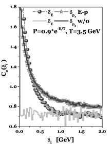
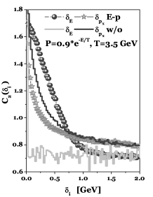
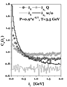
Figure 15: Effects of correcting for the imbalances introduced by our selection procedure in energy-momentum (upper panels and lower-right panel) and total charge (lower panels). Results without ($w/o$) corrections are the same at all panels. Two selection of the $(+/-)$ sign of the $p_{L}$ component are used: it is chosen randomly for each particle irrespective to EEC it belongs to (all panels except the upper-left one); all particles in a given EEC possess $p_{L}$ of the same sign (upper-left panel). In all panels first bin of gray full curve contains uncorrected $C_{2}(\delta_{E})$. In all cases $\sigma_{0}=0$.

conserved by accepting only events reproducing the initially assumed charge. Results of all other algorithms presented here were prepared in the same way as what we have presented, i.e., not corrected for any, therefore they can be compared with each other. We would now like to discuss changes in correlation functions induced by correcting for energy-momentum and charge imbalances introduced in the selection process. At first one must stress that there is no unique procedure to perform such corrections EPQ . In what follows we shall use a very simple (but fast) procedure: $(i)$ - shifting (by the same amounts, $\Delta p_{x}$, $\Delta p_{y}$ and $\Delta p_{z}$) components of momenta, $p_{x,y,z}$ and, after balancing momenta, appropriately rescaling energies; $(ii)$ by converting the necessary number of $(+)$ particles to $(-)$ ones (or vice versa, depending on the actual charge balance in the event) and, in case of odd number of particles with surplus charge, attribute the surplus charge to some randomly chosen $(0)$ charged particle.

Figure 16: Typical distributions of total charges obtained from our selection procedure performed for $W=91.2$ GeV, $T=3.5$ GeV and $\sigma_{0}=0.$ for different sizes of EEC as dictated by parameter $\mathcal{P}_{0}=0.9$ and $\mathcal{P}_{0}=0.3$ and for maximal size of EEC artificially limited to $n_{max}=4$ (for $\mathcal{P}_{0}=0.9$). The best fits to most narrow and most wide distributions are shown. Total initial charge of hadronizing mass $W$ was assumed $Q=0$.

The results are shown in Fig. 15 (our hadronizing sources have zero initial charge). The most sensitive to the correcting procedure is $C_{2}(\delta_{E})$, correlations of momenta feel corrections only when all particles in a given EEC are located in the same hemisphere. Otherwise there is essentially no difference, The reason for such behavior is that in the other case, the relative differences of momenta considered here are not changed by the shifting procedure. In correcting for $\Delta Q\neq 0$ the EECs with single particle only were chosen first, afterwards EECs with $N_{part}>1$ were chosen randomly until the correct balance of charge was achieved. In this case, as one can see in Fig. 15 (lower panels), the effect is quite dramatic and essentially independent of the way the momenta were chosen or on their energy-momentum balance. The best measure of this is provided by the widening of the originally $\delta$-like $C_{2}(\delta_{E})$. Notice also the clearly visible upward bending of the tail of $C_{2}$ distributions. It is worth notice at this point that similar shapes are observed in $C_{2}$ obtained from $e^{+}e^{-}$ annihilation experiments, in which, as in the case considered here, the original energy and total charges are well known and fixed.

Effects shown here are so dramatic because, in order to be as near as possible to the proper BE distributions in the average EEC in situation of only limited energy $W$ available for hadronization, we had maximized sizes of EECs by allocating to them many particles, this was technically achieved by using large value of parameter $\mathcal{P}_{0}$, $\mathcal{P}_{0}=0.9$. It resulted in very broad total charge distribution (centered on the assumed value $Q_{TOT}=0$), see Fig. 16. The reason for such large fluctuations is as follows. In our algorithm each EEC contains particles of the same charge $(+,-,0)$ selected randomly (with equal probabilities). With only one particle per EEC, $N_{part}=1$, this would result in quite narrow $\Delta Q_{EEC}$. However, because in general $N_{part}>1$ and fluctuates, the charge imbalance $\Delta Q_{EEC}$ broadens considerably to what is observed in Fig. 16. It leads then to very large fluctuations and events with large charge imbalance are quite frequent. The effect is therefore, as seen in Fig. 16, very sensitive to the size of EEC allowed (see Fig. 4 and Table 1), i.e., to the parameter $\mathcal{P}_{0}$ responsible for $N_{part}$ and to any attempts to limit it as, for example, shown in Fig. 10 FOOTQ .

To summarize: this problem arises because our procedure destroys part of the originally formed EECs and forms some new ones what results in the sensitivity observed. On the other hand we do not see at the moment any economical way to account for extremely complicated correlations arising when attempting to keep $Q_{TOT}=0$ all the time. The only apparent cure, to keep only events with exactly right charge balance, would place our algorithm in the same category (in what concerns the use of computational time) as those presented in Sects. II.2.1 and II.2.2 zajc ; Cramer (which, by the way, were not attempting to impose any conservation laws at all).

References

- (1) Compare QM05 proceedings, Nucl. Phys. A774 (2006); for specialized reviews see also K.J. Eskola, Nucl. Phys. A698, 78 (2002) or S.A.Bass et al. Prog. Part. Nucl. 41, 255 (1998).
- (2) G. Goldhaber et al., Phys. Rev. Lett 3, 181 (1959), G. Goldhaber et al., Phys. Rev. 120, 300 (1960).
- (3) In fact, at the beginning the observed effect was called GGLP effect in distinction to apparently similar effect observed in astronomy and known as HBT effect which was used to obtain stellar dimensions, see T.J Humanic, Int.J.Mod.Phys. E15, 197 (2006) for most recent review and refernces therein. Other important reviews are in rev whereas pedagogical descriptions of BEC are provided in Z and Weiner . Finally, in WeinerC one can find valuble collection of seminal papers concerning different aspects of BEC.
- (4) U.A. Wiedemann and U. Heinz, Phys. Rep. 319, 145 (1999); R.M. Weiner, Phys. Rep. 327, 249 (2000); T. Csörgő, Acta Phys. Hung., New Series, Heavy Ion. Phys. 15, 1 (2002) and in Particle Production Spanning MeV and TeV Energies, eds. W. Kittel et al., NATO Science Series C, Vol. 554, Kluwer Acad. Pub. (2000), p. 203 [hep-ph/0001233]; W. Kittel, Acta Phys. Polon. B32, 3927 (2001); G. Alexander, Rep. Prog. Phys. 66, 481 (2003).
- (5) W.A. Zajc, A pedestrian’s guide to interferometry, in Particle Production in Highly Excited Matter, eds. H.H.Gutbrod and J.Rafelski, Plenum Press, New York 1993, p. 435.
- (6) R.M. Weiner, Introduction to BEC and subatomic interferometry, Wiley (1999).
- (7) R.M. Weiner, Bose-Einstein correlations in particle and nuclear physics (Collection of selected articles), J.Wiley, (1997).
- (8) W.A. Zajc, Phys. Rev. D35, 3396 (1987).
- (9) It means that the unobserved yield acts as a kind of heath bath influencing measured observables. Actually this is the main origin of the known spectatular success of the statistical description of such reactions with ”temperature” being the most important parameter describing the influence of such a heath bath, see G. Wilk, Fluctuations, correlations and non-extensivity, hep-ph/0610292, to be published in Braz. J. Phys., and references therein.
- (10) G.A. Kozlov, O.V. Utyuzh and G. Wilk, Phys. Rev. C68, 024901 (2003) and Ukr. J. Phys. 48, 1313 (2003).
- (11) Closer inspection Z reveals that one rather gets in this way a Fourier transform of distributions of spatio-temporal two-particle separations (or correlation lengths rev ). Recently the possibility of sort of imaging the hadronization region by using data on has been pursued, see D.A. Brown et al., Phys.Rev. C72, 054902 (2005) and references therein.
- (12) M. Biyajima, N. Suzuki, G. Wilk and Z. Włodarczyk, Phys. Lett. B386, 297 (1996).
- (13) H. Merlitz and D. Pelte, Z. Phys. A357, 175 (1997). Cf. also: U.A. Wiedemann et al., Phys. Rev. C56, R614 (1997); T. Csörgő and J. Zimányi, Phys. Rev. Lett. 80, 916 (1998) and Heavy Ion Phys. 9, 241 (1999).
- (14) H. Merlitz and D. Pelte, Z. Phys. A351, 187 (1995).
- (15) J.G. Cramer, Event Simulation of High-Order Bose-Einstein and Coulomb Correlations, Univ. of Washington preprint (1996, unpublished).
- (16) T. Osada, M. Maruyama and F. Takagi, Phys. Rev. D59, 014024 (1998).
- (17) K. Fiałkowski, R. Wit and J. Wosiek, Phys. Rev. D58, 094013 (1998); T. Wibig, Phys. Rev. D53, 3586 (1996); B. Andersson, Acta Phys. Polon. B29, 1885 (1998); K. Geiger, J. Ellis, U. Heinz and U.A. Wiedemann, Phys. Rev. D61, 054002 (2000); Q.H. Zhang, U.A. Wiedemann, C. Slotta and U. Heinz, Phys. Lett. B407, 33 (1997).
- (18) B. Andersson, M. Ringner, Nucl. Phys. B513, 627 (1998).
- (19) L. Lönnblad and T. Sjöstrand, Eur. Phys. J. C2, 165 (1998).
- (20) O.V. Utyuzh, G. Wilk and Z. Włodarczyk, Phys. Lett. B522, 273 (2001).
- (21) O.V. Utyuzh, G. Wilk and Z. Włodarczyk, Acta Phys. Polon. B33, 2681 (2002).
- (22) O.V.Utyuzh, G.Wilk and Z.Włodarczyk; Bose-Einstein Correlations as correlations of fluctuations, in Proc. of the XXXII ISMD, Alushta, Crimea, Ukraine, September 7-13, 2002; eds. A.Sissakian, G.Kozlov and E.Kolganova, p. 50 [hep-ph/0210328].
- (23) The only discussion of such changes we are aware of is in UWW1 ; UWW2 where it was shown that enforcing effect of BEC into a simple cascade model results in the appeareances of multi-charged vertices, not present in the original scheme. For more details see AIP and references therein.
- (24) O.V.Utyuzh, G.Wilk and Z.Włodarczyk, AIP Conf. Proc. 828, 75 (2006) [hep-ph/0509320]; Nukleonika 49 (Supplement 2), S33 (2004) [hep-ph/0312164]; Acta Phys. Hung. A - Heavy Ion Phys. 25, 83 (2006) 83 [hep-ph/0503046] and Nukleonika 51 (Supplement 3) (2006) S105 [hep-ph/0509342].
- (25) A. Giovannini and L. Van Hove, Z. Phys. C30, 391 (1986); see also: P. Carruthers and C.S.Shih, Int. J. Mod. Phys. A2, 1447 (1987).
- (26) U. A. Wiedemann, P. Foka, H. Kalechofsky, M. Martin, C. Slotta and Q. H. Zhang, Phys. Rev. C56, R614 (1997); M. Martin, H. Kalechofsky, P. Foka and U.A. Wiedemann, Eur. Phys. J. C2, 359 (1998).
- (27) The reason is obvious. When only mean multiplicity is fixed the most probable distribution according to IT approach is geometrical (or Bose-Einstein) one. Such is therefore distribution of particles in each cell in rapidity, therefore their composition will result in of NB type NBD .
- (28) Actually one obtains in this way only some part of this intermittency signal. Nevertheless this fact suggests that fluctuations connected with intermittency Intermitency are, at least to some extent, the same as those caused by BEC (or both have the same origin), cf. P. Carruthers, E.M. Friedlander, C.C. Shih and R.M. Weiner, Phys. Lett. B222, 487 (1989) and Weiner .
- (29) E. A. De Wolf, I. M. Dremin, and W. Kittel, Phys. Rep. 270, 1 (1996); P. Bożek, M. Płoszajczak, and R. Botet, ibid. 252, 101 (1995); I. V. Andreev, I. M. Dremin, M. Biyajima, and N. Suzuki, Int. J. Mod. Phys. A 10, 3951 (1995).
- (30) K. Zalewski, Nucl. Phys. B (Proc. Suppl. 74, 65 (1999) and Lecture Notes in Physics 539, 291 (2000).
- (31) E. E. Purcell, Nature 178, 1449 (1956). Cf. also, L.Mandel, E.C.G.Sudarshan and E.Wolf, Proc. Phys. Soc. 84, 435 (1964).
- (32) A.Giovannini and H.B.Nielsen, Stimulated emission model for multiplicity fluctuations, The Niels Bohr Institute preprint, NBI-HE-73-17 (unpublished). See also: Stimulated emission effect on multiplicity distribution in: Proc. of the IV Int. Symp. on Multip. Hadrodynamics, Pavia 1973, Eds. F.Duimio, A.Giovannini and S.Ratii, p. 538.
- (33) See, for example, R.Loudon, The quantum theory of light ( ed.) Clarendon Press - Oxford, 1983 or J.W.Goodman, Statistical Optics, John Wiley & Sons, 1985.
- (34) Notice that, in general, the multiplicity distribution function satisfies the relation: where is reflection of the fact that with particles given the th one can be allocated in ways. Different result in different forms of . In particular for one gets (after normalization) whereas results (after normalization) in , i.e., in a geometrical distribution, which means that the emission of an extra particle is enhanced by a factor and this is Bose-Einstein enhancement and the emission with this is usually called stimulated emission GN .
- (35) M.Biyajima, Prog. Theor. Phys. 69, 966 (1983) and Phys. Lett. B137, 225 (1984).
- (36) W.J. Knox, Phys. Rev. D10, 65 (1974); E.H. De Groot and H. Satz, Nucl. Phys. B130, 257 (1977); J. Kripfganz, Acta Phys. Polon. B8, 945 (1977); A.M. Cooper, O. Miyamura, A. Suzuki and K. Takahashi, Phys. Lett. B87, 393 (1979); F. Takagi, Prog. Theor. Phys. Suppl. 120, 201 (1995).
- (37) K.Fiałkowski, in Proc. of the XXX ISMD, Tihany, Hungary, 9-13 October 2000, Eds. T.Csörgő et al., World Scientific 2001, p. 357; M.Stephanov, Phys. Rev. D65, 096008 (2002).
- (38) In fact all this is true only for an a priori unlimited number of trials. In reality, because the pool of available particles is (where is limited by the available energy ) one gets and , where is given by eq. (14). It means that eq. (17) will also be modified accordingly.
- (39) R. Kacker and I. Olkin, J. Res. Natl. Inst. Stand. Tech. 110, 67 (2005).
- (40) J. Finkelstein, Phys. Rev. D37, 2446 (1988); Ding-wei Huang, Phys. Rev. D58, 017501 (1998).
- (41) P. Abreu et al. (DELPHI Collab.), Phys. Lett. B286 (1992) 201 and Phys. Lett. B247 (1990) 137.
- (42) It is interesting to notice at this point that the best fits to and for presented here can be obtained by using, respectively ( and ), shifted Gaussian, (with , , and ) and shifted lorentzian, (with , , and ). Notice that the later shape belongs to the category of Lévy distributions discussed in context of BEC in T. Csörgő, S. Hegyi and W. Zajc, Eur. Phys. J. C36 (2004) 36 because of their connection with the possible fractality of the hadronizing source. In fact one could as well use other forms of function in eq. (24) to get still another forms of , see for example, T. Mizoguchi, M. Biyajima and T. Kageya, Prog. Theor. Phys. 91, 905 (1994) (for more details cf. Beyond the Gaussian Approximation chapter in AIP Conf. Proc. 828 (2006))).
- (43) I.V. Andreev, M. Plümer, B.R. Schlei and R.M. Weiner, Phys. Rev. D49 (1994) 1217.
- (44) V.V. Begun and M.I. Gorenstein, Bose-Einstein Condensation of Pions in High Multiplicity Events, hep-ph/0611043; for references to high multiplicity measurement projects see E. Kokoulina, A. Kutov and V. Nikitin, Gluon dominance model and cluster production, hep-ph/0612364, to be published in Braz. J. Phys..
- (45) See, for example, A.M. Gavrilik, Symm., Integ. and Geometry, Meth. and Appl. 2 074 (2006) [hep-ph/0512357] or Ch. A. Nelson and P. R. Shimpi, Hanbury-Brown and Twiss Intensity Correlations of Parabosons, math-ph/0610075.
- (46) This should be contrasted, for example, with the concept of resonant ”halo” discussed in S. Nickerson, T. Csörgő and D. Kiang, Phys. Rev. C57, 3251 (1998), which is not able to do so.
- (47) Notice that the problem of how to account for the possibly nonzero spin of produced resonances is highly nontrivial. In principle, one should build EECs with particles possessing either the same helicity (but then they would all have to possess momenta pointing in the same direction) or with the same projection of spins (but then one would have to choose the external axis and choose not energies, as we are doing so far, but rather momenta). In both cases it would result in a completely different approach, which we shall not pursued here.
- (48) See, for example, O. Pooth (OPAL Collaboration), Nucl. Phys. B (Proc. Suppl.) 152, 35 (2006) and references therein.
- (49) This is a potentially very interesting result deserving further specialized consideration, which, however, would lead us outside the scope of the present paper. In this respect we refer to work by E K.G. Sarkisyan, Phys. Lett. B477, 1 (2000), where different multplicity distributions were studied from the point of view of intermittency and higher-order correlations. Similarly, in G. Abbiendi et al. (OPAL Collab.), Phys. Lett. B523, 35 (2001) one can find studies of intermittency and especially of the higher-order genuine correlations made with all-charge vs. like-sign group of hadrons compared to Bose-Einstein effect.
- (50) A. Kisiel, T. Tałuć, W. Broniowski and W. Florkowski, Comp. Phys. Comm. 174, 669 (2006).
- (51) T. Osada, O.V. Utyuzh, G. Wilk and Z.Włodarczyk, Eur. Phys. J. B50, 7 (2006) and references therein.
- (52) M. Biyajima, T. Mizoguchi, T. Osada and G.Wilk, Phys. Lett. B353, 340 (1995) and 366, 394 (1996); see also review by O.V. Utyuzh, AIP Conf. Proc. 828, 595 (2006).
- (53) Compare, for example, A.E.Ezhov and A.Yu.Khrennikov, Phys. Rev. E71, 016138 (2005); K. Stalinas, Bose-Einstein condensation in dissipative systems far from thermal equilibrium, cond-mat/0001436 and Bose-Einstein condensation in classical systems cond-mat/0001347.
- (54) R. Kutner and M. Regulski, Comp. Phys. Com. 121-122, 586 (1999); cf. also: R. Kutner, K.W. Kehr, W. Renz and R. Przeniosło , J.Phys. A28, 923 (1995).
- (55) G. Bianconi and A.-L. Barabási, Phys. Rev. Lett. 86, 5632 (2001).
- (56) R. J. Glauber, Rev. Mod. Phys. 78, 1267 (2006) and references therein.
- (57) That this point can be important is demonstrated, for example, in: N. Borghini, Eur. Phys. J. C30, 381 (2003) and Momentum conservation and correlation analyses in heavy-ion collisions at ultrarelativistic energies, nucl-th/0612093; B.B. Back, Phys. Rev. C72, 064906 (2005) or in: Z. Chajȩcki and M. Lisa, Global Conservation Laws and Femtoscopy of Small Systems, nucl-th/0612080.
- (58) For example, the sequential choice of energies from the distribution would result in an event reproducing the initial distribution and conserving energy (because sampling from uniform distribution results in , cf., M. Shibata, Phys. Rev. D24, 1847 (1981)). This could be thought as a natural method to follow. However, it turns out that one cannot correct imbalances in momenta just by rotating all angles by some fixed ), the rescaling of at least one component is necessary. This ruins the original energy balance and needs further corrections.
- (59) It is interesting to note that distributions of in Fig. 16 follow Gaussian form for small small , for which becomes the so called -Gaussian distribution (known from Tsallis statistics, see reference in FOOT1 ).