Chuan-Hung Chen1,2***Email:
physchen@mail.ncku.edu.tw and Tzu-Chiang
Yuan3†††Email: tcyuan@phys.nthu.edu.tw1Department of Physics, National Cheng-Kung
University, Tainan 701, Taiwan
2National Center for Theoretical Sciences, Taiwan
3Department of Physics, National Tsing-Hua University, Hsinchu
300, Taiwan
Abstract
Production of , a theoretical endeavor of pure scalar glueball state, is studied in detail
from exclusive rare decay within the framework of perturbative QCD.
The branching fraction for is estimated to be
about , while for it is smaller by roughly
an order of magnitude.
With the accumulation of almost 1 billion pairs from the BABAR
and Belle experiments to date,
hunting for a scalar glueball via these rare decay modes should be attainable.
From the modern point of view, properties of pseudoscalar mesons can
be understood as Nambu-Goldstone bosons due to the spontaneous
symmetry breaking of chiral symmetry. Their low energy dynamics can
be described by the chiral lagrangian. On the other hand, scalar
mesons are not governed by any low energy symmetry like chiral
symmetry and thus they can not take advantage of the power of a
symmetry. Indeed, their classification, the quark content of
their composition, as well as their spectroscopy are not well
understood for scalar mesons scalar-mesons . Moreover,
possible mixings of the states with a pure glueball state
cheng-chua-liu ; he-li-liu-zeng ; close-zhao ; giacosa-etal ; burakovsky-page ; fariborz ; chanowitz-talk must be taken into consideration.
Recent quenched lattice simulation lattice predicted the lowest pure glueball state has
a mass equals MeV and . The first error is statistical while the second is due to approximate anisotropy of the lattice.
This suggests that before mixing, a glueball mass should be closed to 1710 MeV, instead of the
earlier lattice result of 1500 MeV cheng-chua-liu .
This makes a strong candidate for a lowest pure glueball state as advocated in
chanowitz based on argument of chiral suppression
in decays into pair of pseudoscalar mesons.
The next two pure glueball states predicted by the quenched approximation lattice have masses
MeV and MeV
with and respectively.
Mixings between the nearby three isosinglet scalars , , and
and the isovector scalar have been studied in detail in cheng-chua-liu with the following main result:
In the symmetry limit, is a pure octet and degenerate with the isovector scalar meson , whereas
is mainly a singlet with a small mixing with which is composed
predominantly by a scalar glueball.
Important production mechanism of glueballs is the decay of heavy
quarkonium closeetal ; he-jin-ma ; zhao-close .
In fact, the observed enhancement of the mode
relative to and the copious production of
in the radiative decays are strong indication that
is mainly composed of glueball cheng-chua-liu .
Another interesting mechanism is the
direct production from brodsky ,
where stands for a glueball state of spin or 2 and denotes a or
.
Recently, glueball production from inclusive rare decay he-yuan has also been studied.
Ironically, scalar glueball state has never been observed in the gluon-rich channels of decays or collisions333
For a summary of the non- candidates from the Particle Data Group, see p949 of
Ref.pdg .
.
In this article, we will study glueball production via exclusive
decay using perturbative QCD (PQCD).
Firstly, we will
ignore mixing effects and treat as a pure scalar
glueball suggested by the quenched lattice data. At the end of
the paper, we will demonstrate the mixing effects are minuscule.
At quark level, the
effective Hamiltonian for the decay can be written
as BBL
(1)
where denotes the product of Cabibbo-Kobayashi-Maskawa
(CKM) matrix elements and the operators - are
defined as
(2)
with and being the color indices and
- the corresponding Wilson coefficients.
In addition, the gluonic penguin vertex for with
next-to-leading QCD corrections is given by he-lin
(3)
where is the strong coupling constant, is the
-quark mass, is the generator for the color group, and
, and .
Explicit formulas for and can be found in
Ref. GFA . Since the ground state scalar glueball is composed
of two gluons, the effective interaction between a scalar glueball
and gluons can be written as chanowitz
(4)
where stands for an unknown effective coupling constant,
denotes the scalar glueball field, and is the gluon field
strength tensor.
With these 4-quarks operators (2) and the two effective couplings (3) and
(4), we can embark upon the computation of the decay rates for using PQCD.
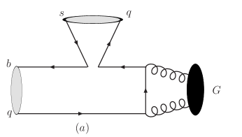
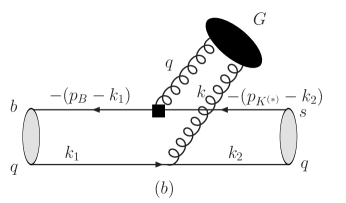
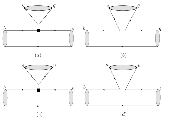
The flavor diagrams for decays are
displayed in Fig. 1.
Fig.(1a) denotes contribution from the 4-quarks operators given
in Eq.(2),
whereas Fig.(1b) involves the gluonic penguin vertex contribution of Eq.(3).
Both diagrams are of the same order in .
In the heavy quark limit, the production of light meson is supposed to respect color transparency Bjorken , i.e., final state interactions are subleading
effects and negligible. We will work under this assumption in what follows.
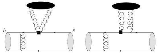
Moreover, diagrams like Fig.2 that are of higher order in will be ignored.
Figure 1: Flavor diagrams for the .
Figure 2: Other flavor diagrams for the at higher order in .
To deal with the transition matrix elements
for exclusive decays, we employ PQCD
PQCD1 ; PQCD2 factorization formalism to estimate the hadronic
effects. By the factorization theorem, the transition amplitude can
be written as the convolution of hadronic distribution amplitudes
and the hard amplitude of the valence quarks, in which the
distribution amplitudes absorb the infrared divergences and
represent the effects of nonperturbative QCD. As usual, the hard
amplitudes can be calculated perturbatively by following the Feynman
rules. The nonperturbative objects can be described by the nonlocal
matrix elements and are expressed as
GN_PRD55 ; K-meson ; KLS_PRD65
(5)
for , , and mesons, respectively, where is the
number of color, are two light-like vectors satisfying ,
and is the longitudinal polarization vector
of .
, the distribution amplitude of meson, is constructed
as follows KLS_PRD65
(6)
with .
and are the
twist-2 and 3 distribution amplitudes of mesons with the argument stands for the
momentum fraction.
Finally, and are the masses for the and with
where and denote the light quark masses.
The meson distribution amplitudes are subjected to the following
normalization conditions
(7)
where
and
and are the decay constants.
We do not introduce transverse momenta for the light mesons and here which we will
justify later when we discuss the end-point singularities of the decay amplitudes.
In the light-cone coordinate system, we can pick the two light-like vectors to be
and ,
and the momenta of the and mesons can be written as
(8)
with .
For the vector meson , we take
(9)
with in which the physical condition
is satisfied for massive vector particle.
The momenta of the spectator quarks with their transverse momenta included are given by
(10)
With these light-cone coordinates and distribution amplitudes defined,
we can study the transition matrix elements for ().
We first analyze Fig. 1(a).
Within the PQCD approach, we find that Fig. 1(a) is directly proportional to .
Since is the momentum fraction
of the valence quark inside the meson and its value is expected
to be with .
Comparing to (Fig. 1(b)), its contribution
belongs to higher power in heavy quark expansion.
As an illustration, we can use the operator in
Eq. (2) to demonstrate this effect. Thus, one finds
where . It has been shown in KLS_PRD65
that under Sudakov suppression arising from and threshold
resummations, the average transverse momenta of valence quarks are
GeV and the end point singularities at
in Eq.(LABEL:ampl-O-4) can be effectively removed.
With an explicit factor of appearing in the numerator of
Eq.(LABEL:ampl-O-4), this contribution is regarded as a higher power
effect in and therefore can be neglected. We note that this
situation is quite similar to the flavor singlet mechanism to the
form factor BN_NPB651 . According to the
PQCD analysis in Ref. Li , contribution from the possible
gluonic component inside to the form
factor also has similar behavior. Its numerical value is two orders
of magnitude smaller than the form factor. Similarly,
other operators and give the same behavior.
Therefore, to the leading power in ,
the contributions from Fig. 1(a) can be neglected. We
will concentrate on the contribution of Fig. 1(b) in
what follows.
By using the introduced nonlocal matrix elements for mesons and the
light-cone coordinates given above, the transition
matrix element for () can be obtained from Fig. 1(b)
as
(12)
with the decay amplitude function given by
(13)
(14)
for the pseudoscalar , and
(15)
for the vector meson . Here we have introduced the
dimensionless variables , , and
.
The hard function in Eq.(13) is given by
(16)
with and
.
The evolution factor in Eq.(13)
is defined by
(17)
where is the Sudakov exponents that resummed
large logarithmic corrections to the meson wave
functions CL_PRD63 ; LL_PRD70 . Their explicit forms are given by
(18)
where is the anomalous dimension.
To leading order in , equals .
The function in Eq.(18) is given by CS ; BS
(19)
where
(20)
with being the active flavor number and is the Euler
constant.
As mentioned before, ,
we have dropped all terms related to in the
above expressions for . Since ,
we have retained only those terms in the above formulas for
that are at most linear in . The
scale where the strong coupling in (17),
the Sudakov exponents in (18),
and the and in (14) are evaluated
will be discussed later.
For comparison, we also present the formula
of the decay amplitude function with in Appendix A.
For estimating our numerical results, we take the values of
theoretical parameters to be: MeV, GeV,
GeV, . For the meson distribution amplitude, we
use CL_PRD63
(21)
with GeV and GeV.
For the distribution amplitudes of the light
pseudoscalar and vector mesons , we refer to their results derived by
the light-cone QCD sum rules in BBL_JHEP ; BZ_PRD71 ; BBKT . Their
explicit expressions and relevant values of parameters are collected
in the Appendix B for convenience.
According to the results
of light-cone QCD sum rules, at small , the behavior of twist-2
distribution amplitude obeys the asymptotic form
, whilst those of twist-3
distribution amplitudes approach a constant
. Consequently,
at small , the decay amplitude function contributed by the
twist-2 distribution amplitudes of behaves like
(22)
Obviously, even if one sets to be zero, the effects from
twist-2 distribution amplitudes of are well-defined at the end point .
Similarly, the contribution from twist-3 distribution amplitudes to the decay amplitude function
at small behaves like
(23)
Whence , one will suffer logarithmic
divergences from the twist-3 distribution amplitudes. In practice,
, the divergence will not occur. This implies that the influence of
can only be mild. As a common practice, we do not introduce
transverse momenta for the valence quarks to suppress large effects from end
point singularities.
Since the Wilson coefficients are scale dependence, for
smearing its dependence, we include the values of Wilson
coefficients with the next-to-leading QCD corrections GFA .
However, even so, the are still slightly
-dependence. Due to this reason, determination of the scale of
exchanged hard gluons in Fig. 1 is also one of the
origins of theoretical uncertainties. For the gluon that attached to
the penguin vertex , it carries a typical momentum of
. When and is
, say , we get GeV. However, the
gluon attached to the spectator quark carries roughly a typical
momentum of GeV. We note that a suitable range of
in PQCD is often taken as . For definiteness, we take
the democratic average value as the
hard scale, in which the allowed value is within the range GeV. This justifies somewhat the validity of the PQCD
approach and we will take this range of as our theoretical
uncertainties. For illustration, we present the involving Wilson
coefficients at different values of scale in
Table 1.
Table 1: The involving Wilson coefficients at various values of scale.
Wilson coefficient
GeV
2.5 GeV
3.0 GeV
Effective interactions between a scalar glueball and the pseudoscalars
have been studied using chiral perturbation theory chao-he-ma ; he-yuan .
By using the current experimental data pdg
MeV and BR,
this allows us to get an estimate of the unknown coupling
GeV-1he-yuan .
This result of should be taken as a crude estimation. For one thing,
the data of the branching ratio BR was not used for averages, fits, limits, etc. by the PDG pdg .
Instead the following two ratios were used in the PDG analysis:
(24)
(25)
Within the approach of chiral perturbation theory he-yuan , it would be difficult to accommodate these two ratios of Eqs.(24) and (25), since the leading term in the chiral Lagrangian is flavor blind. Here we will present another approach to estimate .
At quark level, the amplitude for is proportional to the
quark mass and therefore chirally suppressed. Its explicit form is
given by chanowitz
(26)
where denotes the velocity of the quark and is the
quark (anti-quark) spinor.
It has been argued in chanowitz that the chiral suppression
of the amplitude persist in all order of .
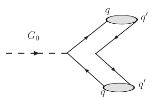
One may treat the coefficient of this decay amplitude
as the short-distance coefficient of the strong decay where stands for
a pseudoscalar meson like , , or etc, as illustrated in Fig. 3.
Thus,
(27)
with, to leading order in ,
(28)
and is the time-like form factor
evaluated at .
Figure 3: Flavor diagram for the with being a
pseudoscalar.
For the case of , we include the quark-flavor mixing effect
according to and with
, flavor0 ; flavor , and KLOE .
Using Eq. (27), the following ratios of the partial decay rates can be obtained
(29)
By taking the flavor approximation, one finds that , , and
. With ,
, , pdg , ,
flavor (all in unit of MeV), one deduces
(30)
Identifying to be , these ratios
are consistent with the current experimental data
quoted in Eqs.(24) and (25).
Using Eq. (26), the following expression of can be
obtained
(31)
where MeV is identified as the width of .
The time-like form factor has been extracted in Ref. CCS
by performing the data fitting to non-resonant decays with the following form
(32)
where , GeV,
GeV2, GeV4,
GeV2, , GeV, and GeV-2. By using
BR pdg , the value for is estimated to be ,
which is only slightly larger than the value obtained from the chiral
Lagrangian approach.
In passing, we note that, using light-cone distribution amplitudes, it has been argued in Ref.chao-he-ma that might be dominated by the 4-quark process of which is not chirally suppressed. Using this 4-quark mechanism and PQCD factorization scheme, one would predict a large ratio of . For further discussion of this issue, we refer our reader to Refs.chao-he-ma ; chao-he-ma-comment ; chanowitz-reply .
Table 2: Decay amplitude (in units of ) for
with and without at
GeV-1 and three different choices of ,
, and GeV. Numbers given in brackets are without
.
Mode
GeV
2.5 GeV
3.0 GeV
Using the matrix element defined by Eq. (13) with the
above chosen values of parameters, the values of are given in Table 2 for
GeV-1 and three different values of scale. For
comparisons, we also present the results with
in Table 2.
The branching fractions for decays are tabulated in Table 3.
From Table 3, we find that the branching fraction for
is about one order of magnitude larger than
that for . The difference arises not only from the
values of the decay constants and entered in the
distribution amplitudes, but also from the effects of
and
in the mode, which are
switched to and
respectively in the
mode.
We also find that the
influence on decay is stronger than . In addition, when is smaller, has lesser effects on
the decay .
Table 3: Branching fractions (in units of ) for with and without at
GeV-1 and three different choices of ,
, and GeV. Numbers given in brackets are without
.
Mode
GeV
2.5 GeV
3.0 GeV
The branching fractions for the decay chains
and are tabulated in Table 4,
where the errors are coming from the experimental data of
BR. From Table 4, we learn
that one has a better chance to look for the ground state of
glueball through the three-body decays , since
its branching fraction could be more than a factor of 10 larger than
.
Table 4: Branching fractions (in units of ) for
at , , and GeV. Numbers given in brackets are without
.
Mode
GeV
2.5 GeV
3.0 GeV
Recently, BABAR had reported the following branching ratio for where
the pair coming from the
babar-br
(33)
From the first and second rows in Table 4, identifying to be , one can see that our predictions are consistent with the experimental data.
Before we close, we want to address the issue of mixing effects.
Although we have treated as a pure
gluonic state, it should be interesting to consider its mixing
effects with other states.
To deal with the mixture of a pure glueball with the quarkonia state,
we follow Ref. cheng-chua-liu to express the state
as the following combination
(34)
where is the pure glueball state,
, and .
Accordingly to one of the mixing schemes cheng-chua-liu ,
the coefficients took the following values:
, , and .
The quoted results of these coefficients are similar
to those obtained by others in Refs. burakovsky-page ; LW . The
corresponding flavor diagrams for the decays
are shown in Fig. 4.
Figure 4: Flavor diagrams for the . (a) and (b)
are from QCD and electroweak penguin diagrams, while (c) and (d)
denote the tree contributions.
Since the distribution amplitude and decay constant for
are uncertain, for simplicity, we use factorization
assumption to estimate the hadronic effects for these two-body
decays. In terms of the operators in Eq. (2),
one can easily show that the contributions from diagram
Fig. 4(a) and (d) are associated with the matrix element
.
Since the scalar or is -even while is -odd,
the contributions from Fig. 4(a) and (d) must vanish
because charge conjugation is a good quantum number in strong interaction.
On the other hand, the contributions from Fig. 4(b) and (c) are non-vanishing and they can be derived as
(35)
(36)
(37)
(38)
for and decays,
respectively,
where , , and are defined by
(39)
is the electric charge of quark and with
and correspond to the form
factors parametrized by CG_PRD75 ; LF1
(40)
and are two other form factors that are not relevant in our analysis.
With GeV, , , , GeV, GeV
cheng-chua-liu , ,
, ,
LF1 , and MeV
CCY , one has the following estimation
(41)
(42)
Comparing these values to those coming from the contribution of purely gluonic state
given in Table 2,
one can conclude that the quarkonia contributions
can be safely ignored.
In summary, we have studied the scalar glueball production in
exclusive decays by using PQCD factorization approach. The
typical momenta carried by the exchanged gluons in the process is
about half of the meson mass. One thus expects our perturbative
results are trustworthy. According to our analysis, we find that
the branching fraction for is a few ;
however, for it can be as large as . As a result, the branching fraction for the
decaying chain
is .
With the experimental inputs of Eqs.(24) and (25),
we also expect the branching ratios for and
are about 50% and less than 10% of
respectively.
In this work, we have focused
on the charged mesons. Similar conclusions can be drawn for the
neutral mesons where the only difference is their lifetimes.
Their mass difference is merely MeV pdg and will not affect our numerical results
significantly. Thus dividing the branching fractions given in Table
3 and Table 4 by the ratio
pdg from direct
measurements, one would obtain the corresponding branching fractions
for the neutral meson modes.
Experimentally,
the mode has been detected at BABAR with a branching ratio
consistent with our PQCD prediction.
This work suggests that detection of the resonant
three-body mode with a predicted larger branching ratio
can give further support of is a pure scalar glueball.
Appendix A Decay amplitude function with
Since the mass of glueball is much larger than those of ordinary
pseudoscalars, we find that the influence of transverse momentum on the two-body
decay
is not as large as in the case of decays into two lighter mesons.
Setting and
in the momenta of the spectator quarks in Eq.(8)
to be zero,
the decay amplitude function given in Eq.(13)
can be simplified to be
(43)
with the hard function given by
(44)
Appendix B Distribution Amplitudes for
In this appendix, we compile the light-cone distribution amplitudes that
entered in our calculations.
The distribution amplitudes for , defined in Eq. (5),
are expressed as follows BBL_JHEP :
(45)
where and the Gegenbauer Polynomials are
given by,
(46)
The coefficients are defined as
(47)
with being the mass of or since is assumed.
Since , in our numerical estimations, we take
.
We display the values of decay constant, mass of strange quark, and
relevant coefficients of distribution amplitudes for meson at GeV
in Table 5.
Table 5: The decay constant, mass of strange quark (in units of
MeV) and coefficients of distribution amplitudes for meson at
GeV.
160
120
0.06
0.25
0.016
Similarly, the distribution amplitude for can be expressed as
BZ_PRD71 ; BBKT
(48)
The values of the decay constants and relevant coefficients of the
distribution amplitudes for the meson are shown in Table 6.
Table 6: The decay constants (in units of MeV) and coefficients of
distribution amplitudes for meson at GeV.
210
170
0.10
0.09
0.13
0.024
0.24
Acknowledgments
This work is supported in part by the National Science Council of
R.O.C. under Grant Nos.
NSC-95-2112-M-006-013-MY2 and
NSC-95-2112-M-007-001 and
by the National Center for Theoretical Sciences.
References
(1)
N. Mathur, A. Alexandru, Y. Chen, S. J. Dong, T. Draper, I. Horvath, F. X. Lee, K. F. Liu, S. Tamhankar, and
J. B. Zhang, arXiv:hep-ph/0607110.
(2)
H. Y. Cheng, C. K. Chua, and K. F. Liu,
Phys. Rev. D 74 (2006) 094005 [arXiv:hep-ph/0607206].
(3)
X. G. He, X. Q. Li, X. Liu, and X. Q. Zeng, Phys. Rev. D 73 (2006) 051502,
ibid. D 73 (2006) 114026.
(4)
F. E. Close and Q. Zhao, Phys. Rev. D 71 (2005) 094022.
(5)
F. Giacosa, Th. Gutsche, V. E. Lyubovitskij, and A. Faessler, Phys. Rev. D 72 (2005) 094006.
(6)
L. Burakovsky and P. R. Page, Phys. Rev. D 59 (1998) 014022.
(7)
A. H. Fariborz, Phys. Rev. D 74 (2006) 054030
[arXiv:hep-ph/0607105].
(8)
M. Chanowitz, Int. J. Mod. Phys. A21 (2006) 5535 [arXiv:hep-ph/0609217].
(9)
Y. Chen, A. Alexandru, S. J. Dong, T. Draper, Horv th, F. X. Lee, K. F. Liu, N. Mathur, C. Morningstar,
M. Peardon, S. Tamhankar, B. L. Yang, and J. B. Zhang,
Phys. Rev. D 73 (2006) 014516 [arXiv:hep-lat/0510074].
(10)
M. S. Chanowitz,
Phys. Rev. Lett. 95 (2005) 172001 [arXiv:hep-ph/0506125].
(11)
C. Amsler and F. E. Close, Phys. Lett. B 353 (1995) 385 [arXiv:hep-ph/9505219],
Phys. Rev. D 53 (1996) 295 [arXiv:hep-ph/9507326];
F. E. Close, G. R. Farrar, and Z.-p. Li, Phys. Rev. D 55 (1997) 5749 [arXiv:hep-ph/9610280].
(12)
X. G. He, H. Y. Jin, and J. P. Ma,
Phys. Rev. D 66 (2002) 074015 [arXiv:hep-ph/0203191].
(13)
Q. Zhao and F. E. Close,
Int. J. Mod. Phys. A 21 (2006) 821 [arXiv:hep-ph/0509305].
(14)
S. Brodsky, A. S. Goldhaber, and J. Lee, Phys. Rev. Lett. 91 (2003) 112001.
(15)X. G. He and T. C. Yuan,
arXiv:hep-ph/06121082.
(16)
Review of Particle Physics, Particle Data Group, J. Phys. G: Nucl. Part. Phys. 33 (2006) 1.
(17) G. Buchalla, A. J. Buras, and M. E. Lautenbacher, Rev.
Mod. Phys. 68 1125 (1996).
(18)
X. G. He and G. L. Lin,
Phys. Lett. B 454 (1999) 123.
(19) Y. H. Chen, H. Y. Cheng, B. Tseng, and K. C. Yang, Phys. Rev D 60
(1999) 094014.
(20) J. D. Bjorken, Nucl. Phys. Proc. Suppl. 11 (1989) 325.
(21)
G. P. Lepage and S. J. Brodsky, Phys. Lett. B 87 (1979) 359, Phys. Rev. D 22 (1980) 2157;
H. N. Li and G. Sterman, Nucl. Phys. B 381 (1992) 129;
G. Sterman, Phys. Lett. B 179 (1986) 281, Nucl. Phys. B 281 (1987) 310;
S. Catani and L. Trentadue, Nucl. Phys. B 327 (1989) 323, Nucl. Phys. B 353 (1991) 183.
(22)
T. W. Yeh and H. N. Li, Phys. Rev. D 56 (1997) 1615;
H. N. Li, Phys. Rev. D 64 (2001) 014019;
H. N. Li, Phys. Rev. D 66 (2002) 094010.
(23)
A. G. Grozin and M. Neubert, Phys. Rev. D 55 (1997) 272.
(24)
V. M. Braun and I. E. Filyanov, Z Phys. C 48 (1990) 239;
P. Ball, JHEP 01 (1999) 010.
(25)
T. Kurimoto, H. N. Li, and A. I. Sanda, Phys. Rev. D 65 (2002) 014007.
(26) M. Beneke and M. Neubert, Nucl. Phys. B
651(2003) 225.
(27)
Y. Y. Charng, T. Kurimoto, and H. N. Li,
Phys. Rev. D 74 (2006) 074024.
(28)
C. H. Chen and H. N. Li, Phys. Rev. D 63 (2000) 014003.
(29) H. N. Li and H. S. Liao, Phys. Rev. D 70
(2004) 074030.
(30) J. C. Collins and D. E. Soper, Nucl. Phys. B 193 (1981) 381.
(31) J. Botts and G. Sterman, Nucl. Phys. B 325 (1989) 62.
(32)
P. Ball, V. M. Braun, and A. Lenz, JHEP 05 (2006) 004.
(33)
P. Ball and R. Zwicky, Phys. Rev. D 71 (2005) 014029.
(34)
P. Ball, V. M. Braun, Y. Koike, and K. Tanaka, Nucl. Phys. B 529 (1998) 323.
(35)
K. T. Chao, X. G. He, and J. P. Ma, hep-ph/0512327.
(36)
J. Schechter, A. Subbaraman, and H. Weigel,
Phys. Rev. D 48 (1993) 339.
(37)
T. Feldmann, P. Kroll, and B. Stech, Phys. Rev. D 58, (1998) 114006;
Phys. Lett. B 645 (2007) 197;
A. G. Akeroyd, C. H. Chen, and C. Q. Geng, Phys. Rev. D 75 (2007) 054003.
(38) F. Ambrosino et al. (KLOE Collaboration),
arXiv:hep-ex/0612029.
(39) H. Y. Cheng, C. K. Chua, and A. Soni, arXiv:0704.1049;
Phys. Rev. D 72 (2005) 094003.
(40)
K. T. Chao, X. G. He, and J. P. Ma,
Phys. Rev. Lett. 98 (2007) 149103 [arXiv:hep-ph/0704.1061].
(41)
M. Chanowitz, Phys. Rev. Lett. 98 (2007) 149104 [arXiv:hep-ph/0704.1616].
(42)
B. Aubert et al. (BABAR Collaboration), Phys. Rev. D 74 (2006) 032003.
(43) W. Lee and D. Weingarten, Phys. Rev. D 61 (1999)
014015.
(44) C. H. Chen and C. Q. Geng, Phys. Rev. D 75 (2007) 054010.
(45) H. Y. Cheng, C. K. Chua, and C. W. Hwang, Phys. Rev. D 69 (2004) 074025.
(46) H. Y. Cheng, C. K. Chua, and K. C. Yang, Phys. Rev. D 73 (2006) 014017.