Global analysis of solar neutrinos ( assumed to be Majorana particles ) together with the new KamLAND data in the RSFP framework

Abstract

Assuming neutrinos are Majorana particles having non-zero transitionmagnetic moments, a global analysis of solar neutrino data, together with the new KamLAND data, is presented in the resonant spin flavor precession (RSFP) framework. We used Wood-Saxon and Gaussian shaped magnetic field profiles throughout the entire Sun. For each magnetic field profile, allowed regions from solar data combined with new KamLAND data are examined at 95% confidence level (CL). We showed that all allowed regions are in the large mixing angle (LMA) region and remain the same as the $\mu B$ value is increased for both magnetic field profiles, contrary to the Dirac case studied in our previous work. The electron antineutrino flux from the Sun is calculated, and via the results obtained several limits are set for $\mu B$.

1.Introduction

The magnetic moment solution to solar neutrino problem is alternative possible mechanism to MSW $\left[1-2\right]$ neutrino oscillation solutions. In this solution motivated by Okun $et$ $al$ (OVV) $\left[3\right]$, strong magnetic field in the Sun changes neutrino’s helicity which has non-zero transition magnetic moment, as it passes through a region with the magnetic field. Shortly after this solution was proposed, resonance spin flavor precession (RSFP) was proposed by Lim and Marciano $\left[4\right]$. In the RSFP scenario, there is a combined effect of matter and magnetic field in the Sun on neutrino’s spin and flavor precession. Thus, the neutrino’s spin and flavor flip simultaneously. In other words, left-handed electron neutrinos convert to right-handed neutrinos of other types: $\nu_{e_{L}}\rightarrow$ $\nu_{\mu_{R}}$ or $\nu_{\tau_{R}}$. In the Majorana case $\nu_{\mu_{R}}$ is $\left(\nu_{\mu_{L}}\right)^{C}$ with C being the charge-conjugation and called $\overline{\nu}_{\mu}$. Matter-enhanced spin-flavor precession of solar neutrinos with transition magnetic moments for chlorine and gallium experiments was investigated in detail by Balantekin $et$ $al$ $\left[5\right]$ for Majorana and Dirac case. Raghavan $et$ $al$ investigated solar antineutrinos and gave the theoretical framework for the solar antineutrino flux calculation $\left[6\right]$. In literature, one can find other studies about the solar antineutrino and the experimental limit on its flux $\left[7-10\right]$. In $[7]$, observation of the antineutrinos originated from ${}^{8}B$ neutrinos in the Sun discussed and upper limits on the antineutrino flux are obtained. They used the angular distribution of positrons emitted in the reaction of the inverse beta decay. Obtaining positrons is a signal for the electron antineutrinos. In that study, to find the upper limit, statistics of Super Kamiokande (SK) and directionality of positrons from inverse beta decay were taken into account. In $[8]$, another bound on the antineutrino flux was obtained using SK solar data. The antineutrinos contribution to the SK background and angular variations of them lead us to set an upper bound on the antineutrino flux. To get a more accurate limit, positron angular distribution and antineutrino asimetry was investigated. Gando $et$ $al$ $[9]$ gave experimental results for the antineutrino flux. Their limits is $0.8\%$ $(90\%CL)$ of the Standart Solar Models’ neutrino flux. Miranda $et$ $al$ $[10]$ discussed spin flavor precession effect on solar neutrinos assumed to be Majorana particle. From the KamLAND $[11]$ constraint on the solar antineutrino flux, they put a limit on the Majorana neutrino transition magnetic moment.

In this work, assuming the fact that all neutrinos are Majorana particles, we present a global analysis of solar data combined with the new KamLAND data $\left[12\right]$ in the RSFP scenario. We obtain allowed regions by using standart least squares analysis on the oscillation parameter space, $\Delta m^{2}$ and $\tan^{2}\theta$, space. Our results showed that all allowed regions are in the large mixing angle (LMA) region and have the same chi-square value as $\mu B$ value is increased for both magnetic field profiles. After the combined analysis of solar and KamLAND data, we examine the electron antineutrino flux at certain $\Delta m^{2}$ and $\tan^{2}\theta$ values.

This paper is divided as fallows: in section 2 we give general information on the evolution equation of Majorana neutrinos having transition magnetic moment. In section 3 the relevant magnetic field profiles are given. Detailed statistical analysis are given in section 4. In section 5 a theoretical framework is given for the calculation of the solar antineutrino flux. Finally, our results and conclusion are presented in section 6.

2. Evolution equation for Majorana neutrinos in the RSFP framework

For two generations, Majorana neutrino flavors are $\nu_{e}$ , $\nu_{\mu}$ , $\overline{\nu}_{e}$ , $\overline{\nu}_{\mu}$ . Altough Dirac neutrinos have diagonal and off-diagonal magnetic moments, Majorana neutrinos have only off-diagonal (transition) magnetic moments. For the Majorana neutrinos that propagate through matter and in a transverse magnetic field $B$, the evolution equation in the case of two generations is

$$i\frac{d}{dt}\left[\begin{array}[]{c}\nu_{e}\\ \nu_{\mu}\\ \overline{\nu}_{e}\\ \overline{\nu}_{\mu}\end{array}\right]=H\left[\begin{array}[]{c}\nu_{e}\\ \nu_{\mu}\\ \overline{\nu}_{e}\\ \overline{\nu}_{\mu}\end{array}\right]$$ (1)

where $H$ is given by

$$H=\left[\begin{array}[]{cccc}V_{e}&\frac{\Delta m^{2}}{4E}\sin 2\theta&0&\mu^{\ast}B\\ \frac{\Delta m^{2}}{4E}\sin 2\theta&\frac{\Delta m^{2}}{2E}\cos 2\theta+V_{\mu}&-\mu^{\ast}B&0\\ 0&-\mu B&-V_{e}&\frac{\Delta m^{2}}{4E}\sin 2\theta\\ \mu B&0&\frac{\Delta m^{2}}{4E}\sin 2\theta&\frac{\Delta m^{2}}{2E}\cos 2\theta-V_{\mu}\end{array}\right]$$ (2)

The matter potentials for a neutral unpolarized medium are given as

$$V_{e}(t)=\frac{G_{f}}{\sqrt{2}}(2N_{e}-N_{n})\text{ \ \ \ \ \ \ }V_{\mu}=-\frac{G_{f}}{\sqrt{2}}N_{n}$$ (3)

where $N_{e}$ and $N_{n}$ are electron and neutron number densities in the Sun, respectively, and the $G_{f}=1.16636\times 10^{-5}GeV^{-2}$. In addition in the Sun electron and neutron number densities are well approximated by $N_{e}\simeq 6N_{n}\simeq 2.4\times 10^{26}\exp(-r/0.09R_{\odot})cm^{-3}$ $\left[13\right]$.

One can find $\nu_{e}\rightarrow\overline{\nu}_{\mu}$ resonance from the Hamiltonian through the evolution equation. The spin-flavor conversion submatrix for this transition is given by

$$\left(\begin{array}[]{cc}V_{e}&\mu^{\ast}B\\ \mu B&\frac{\Delta m^{2}}{2E}\cos 2\theta-V_{\mu}\end{array}\right)$$ (4)

Thus $\nu_{e}\rightarrow\overline{\nu}_{\mu}$ resonance condition is

$$N_{e}=\frac{6\sqrt{2}}{10G_{f}}\frac{\Delta m^{2}}{2E}\cos 2\theta$$ (5)

using the aproximation $N_{e}\simeq 6N_{n}$. This value for the electron density required for $\nu_{e}\rightarrow\overline{\nu}_{\mu}$ resonance of Majorana neutrinos is greater than the corresponding value in the Dirac case. The concequences of this difference will be seen in the allowed regions behaviour in the neutrino oscillation parameter space. In our analysis, we find results numerically by diagonalizing the Hamiltonian in equation (2). The relevant method was discussed in $[5]$.

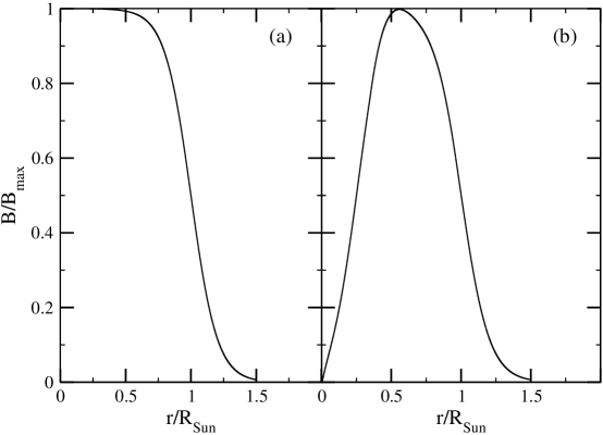
Figure 1: Magnetic field profiles: (a) Wood-Saxon shape; (b) Gaussian shape.

3. Magnetic field profile

In the literature, various magnetic field profiles have been examined from different aspects$\left[14-18\right]$. Here we considered only two as typical for our analysis (see figure 1).

First, we took the magnetic field profile to be a Wood-Saxon shape of the form

$$B(r)=\frac{B_{0}}{1+\exp[10(r-R_{\odot})/R_{\odot}]}$$ (6)

where $B_{0}$ is the strength of the magnetic field at the center of the Sun.

The next magnetic field profile used in the analysis is of Gaussian shape.

4. Statistical analysis

For completeness, we repeat the basics of the statistical methods of our previous work. In this case, however, the relevant processes are to be made carefully. In the literature, there is a common method often called $\chi^{2}$ analysis to find the values of the neutrino oscillation parameters $\Delta m^{2}$, $\tan^{2}\theta$ and to calculate the confidence levels of allowed regions and the goodness of a fit $\left[19-22\right]$. In our analysis, we use ”covariance approach” to find the allowed regions mentioned above. By this method, one minimizes the least-squares function

$$\chi_{{}_{\odot}}^{2}=\sum_{i_{1},i_{2}}^{N_{\exp}}(R_{i_{1}}^{(\exp)}-R_{i_{1}}^{(thr)})(V^{-1})_{i_{1}i_{2}}(R_{i_{2}}^{(\exp)}-R_{i_{2}}^{(thr)})$$ (7)

where $V^{-1}$ is the inverse of the covariance matrix of experimental and theoretical uncertainties, $R_{i}^{(\exp)}$ is the event rate calculated in the $i$th experiment and $R_{i}^{(thr)}$ is the theoretical event rate for the $i$th experiment. The indices indicate the solar neutrino experiments: $i,i_{1},i_{2}=1,...,N_{\exp}$ with $N_{\exp}=4$.

Details of the expressions for theoretical event rates for all solar neutrino experiments, chlorine experiments(Homestake) $\left[23\right]$, gallium experiments (SAGE, GALLEX, GNO) $\left[24-26\right]$, Super Kamiokande $[27]$ and SNO $[28,29]$ are given in $[30]$.

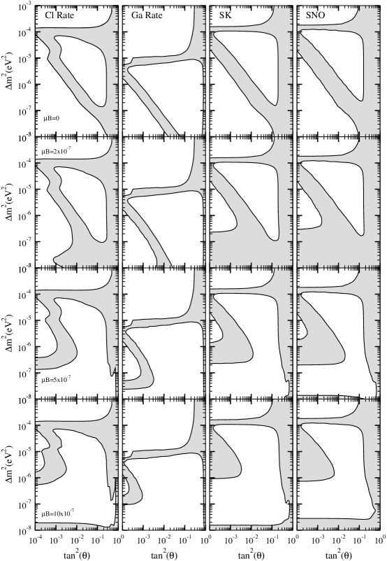
Figure 2: The allowed regions for the Majorana case of neutrino parameter space for each solar neutrino experiment seperately at $\mu B=0,2,5,10\times 10^{-7}\mu_{B}G$ and at 95% CL. Each column and row are for the same experiment and at the same $\mu B$ value,respectively(e.g. in the second row at third column, an allowed region for SK experiment at $\mu B=2\times 10^{-7}\mu_{B}G$ is seen)

For the global analysis, we need $\chi_{KamLAND}^{2}$ $[12,31,32]$

$$\chi_{gl}^{2}=\chi_{{}_{\odot}}^{2}+\chi_{{}_{KamLAND}}^{2}$$ (8)

We took fluxes and cross sections for event rates and error matrices from Bahcall $[33]$.

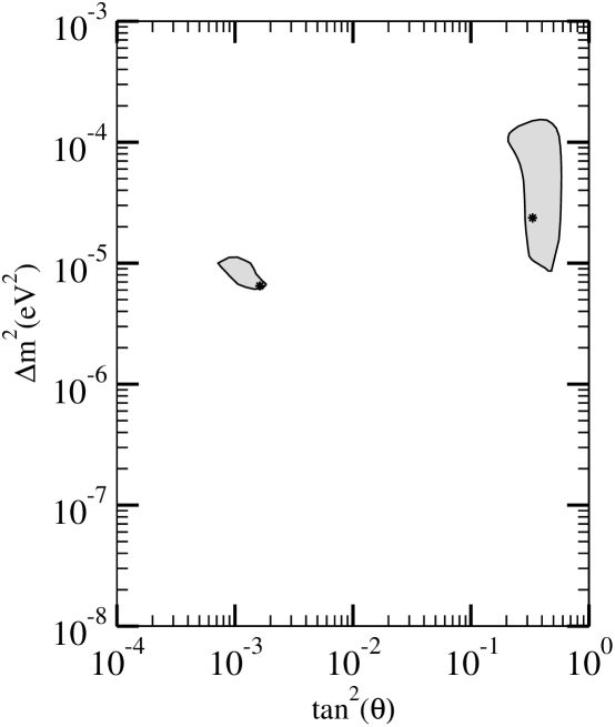
Figure 3: The allowed regions from combined solar neutrino experiments( chlorine, all three gallium, SK and SNO experiments) at the same $\mu B$ values and CL as in figure 2. Stars indicate the local best-fit points.

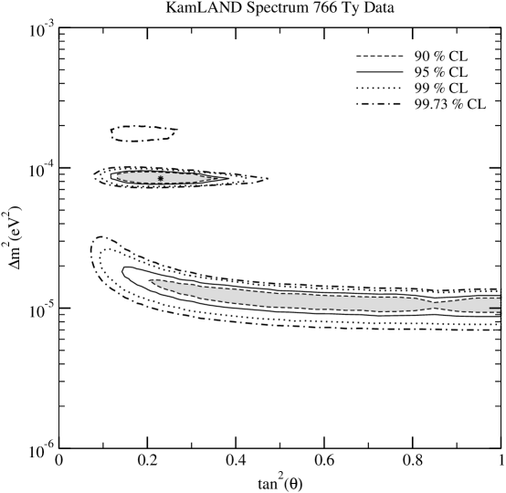
Figure 4: Allowed region from the new KamLAND spectrum at different confidence levels. Star indicates the best fit point.

5.Solar electron antineutrino flux

If neutrinos are Majorana type, $\nu_{e}$ changes to $\overline{\nu}_{\mu}$ inside the Sun by SFP. After Sun, vacuum oscillation yields $\overline{\nu}_{\mu}\rightarrow$ $\overline{\nu}_{e}$. This process is given schematically:

$$\nu_{e}\overset{B_{Sun}}{\rightarrow}\overline{\nu}_{\mu}\overset{V_{osc}}{\rightarrow}\overline{\nu}_{e}$$

To find the electron antineutrino flux on Earth, one need to probability of $\nu_{e}\rightarrow\overline{\nu}_{e}$ transition, $P(\nu_{e}\rightarrow\overline{\nu}_{e})$:

$$P(\nu_{e}\rightarrow\overline{\nu}_{e})=P(\nu_{e}\rightarrow\overline{\nu}_{\mu};SFP)\times P(\overline{\nu}_{\mu}\rightarrow\overline{\nu}_{e};VacuumOsc.)$$

where $\nu_{e}\rightarrow\overline{\nu}_{\mu}$ transition probability $P(\nu_{e}\rightarrow\overline{\nu}_{\mu};SFP)$ is calculated numerically from the equation (2). $P(\overline{\nu}_{\mu}\rightarrow\overline{\nu}_{e};VacuumOsc.)$ is the well known vacuum oscillation probability given as

$$P(\overline{\nu}_{\mu}\rightarrow\overline{\nu}_{e};VacuumOsc.)=\sin^{2}2\theta\sin^{2}(\frac{\Delta m^{2}}{4E}R)\overset{averaging}{\rightarrow}\frac{1}{2}\sin^{2}2\theta$$

where R is the distance between Sun and Earth.

Electron antineutrinos is detected observing the positron from the $\overline{\nu}_{e}+p\rightarrow e^{+}+n$ reaction. Positron event rate is found from

$$N=Q_{0}\int dE_{V}\int\epsilon(E_{e})R(E_{V},E_{e})\Phi_{\overline{\nu}_{e}}(E)\sigma(E)dE$$

where $Q_{0}$ is a normalization constant taking into account the number of atoms in the fiducial volume of the detector and its live time exposure. Positron energy $E_{e}$ is

$$E_{e}=E-1.293MeV$$

and visible energy, $E_{V}=E_{e}+m_{e}$. $\epsilon(E_{e})$ and $R(E_{V},E_{e})$ are the detection efficiency and the energy resolution function of detector, respectively. $\sigma(E)$ is the antineutrino cross section and $\Phi_{\overline{\nu}_{e}}(E)$ is the electron antineutrino flux given by

$$\Phi_{\overline{\nu}_{e}}(E)=\Phi_{\nu_{e}}(^{8}B)\times P(\nu_{e}\rightarrow\overline{\nu}_{e})$$

6.Results and conclusions

In our calculations, we assumed that the magnetic field extends over the entire Sun for both magnetic field profiles. All of the calculations have been performed for both of the magnetic field profiles. Neutrino spectra are taken from the Standard Solar Model of Bahcall and his collaborators $\left[33\right]$. All allowed regions were calculated at 95% CL in this work.

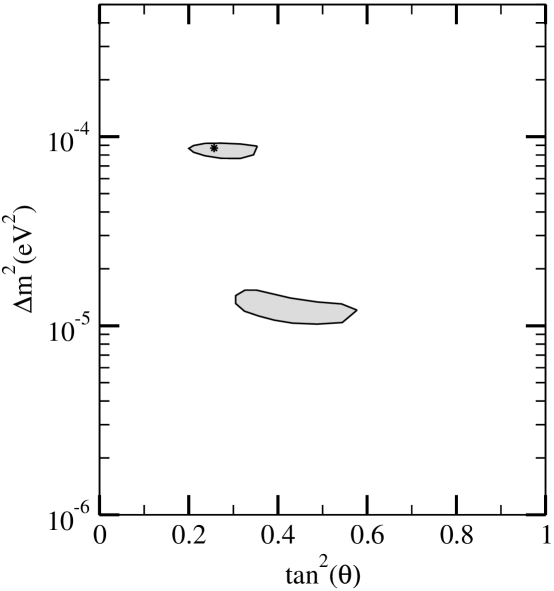
Figure 5: Allowed regions from the combined solar plus new KamLAND spectrum analysis at different $\mu B$ values ($\mu B=0,2,5,10\times 10^{-7}\mu_{B}G$)and at 95% CL. Regions and the best fit point remined the same for all $\mu B$ values. The star indicates the best fit point.

First, we considered only solar neutrino data assuming neutrinos are Majorana type and examined allowed regions for all solar neutrino experiments ( Homestake, Gallium, Super-Kamiokande (SK) and SNO ) using covariance approach of statistical analysis. These results are shown in Figure 2 in which each column and row are for the same experiment and at the same $\mu B$ value respectively(e.g. in the second row at third column, an allowed region for SK experiment at $\mu B=2\times 10^{-7}\mu_{B}G$ is seen).

We displayed the allowed regions from combined solar neutrino experiments in Figure 3. In that figure for both magnetic field profiles, two local best fit points are shown for $\mu B$ values that are $0,2,5,10\times 10^{-7}\mu_{B}G$. The best fit points are at (  $tan^{2}\theta=1.63\times 10^{-3}$, $\Delta m^{2}=6.49\times 10^{-6}$eV² ) for $\mu B$ = $0,2,5\times 10^{-7}\mu_{B}G$ and (  $tan^{2}\theta=1.41\times 10^{-3}$, $\Delta m^{2}=6.49\times 10^{-6}$eV² ) for $\mu B$ = $10\times 10^{-7}\mu_{B}G$, respectively.

After this step, we examined the new KamLAND data and displayed allowed regions from new binned KamLAND data $[12]$ in Figure 4.

As a next stage, our global analysis combining solar and KamLAND spectrum analysis were shown in Figure 5 for the same $\mu B$ values in Figure 2. Regions and the best fit point remained the same for those $\mu B$ values, such that, the best fit point is at  $tan^{2}\theta=0.26$ and at $\Delta m^{2}=8.66\times 10^{-5}$eV². All minimum chi-squares also remained the same for those $\mu B$ values.

It was observed that there are no appreciable differences between the results for the two magnetic field profiles we used; we have given only the figures for Gaussian case.

In contrast to Dirac case $[34]$ in the Majorana case we investigated in this paper, it seems that there is no appreciable magnetic field effect on the allowed regions for Majorana neutrinos in our calculations.

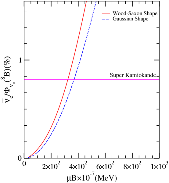
Figure 6: Expected $\overline{\nu}_{e}/\Phi_{\nu_{e}}(^{8}B)$ for $\mu B$ values. The horizantal line shows the upper $\overline{\nu}_{e}/\Phi_{\nu_{e}}(^{8}B)$ flux limit at SK.

Finally to put an upper limit on $\mu B$ for Majorana neutrinos, finally, we calculated resulting electron antineutrino flux from the Sun and compared with the limit obtained by Super Kamiokande. Our results are given in $\overline{\nu}_{e}/\Phi_{\nu_{e}}(^{8}B)-\mu B$ plane for 8-20 MeV visible energy region and at best fit parameters $tan^{2}\theta=0.41$, $\Delta m^{2}=7.1\times 10^{-5}$eV${}^{2}[35]$ in Figure 6. In that figure, the horizantal line shows the upper $\overline{\nu}_{e}/\Phi_{\nu_{e}}(^{8}B)$ flux limit at SK $[9]$. From that limit, one can put a bound on $\mu B$ at these values of $\Delta m^{2}$ and $tan^{2}\theta$. From our results, $\mu B<3.2\times 10^{-5}\mu_{B}G$ and $\mu B<3.7\times 10^{-5}\mu_{B}G$ for Wood-Saxon and Gaussian shaped magnetic field profiles, respectively.

Acknowledgments

We would like to thank to Prof.Dr. A. Baha Balantekin for his suggestions and for his kind help.

References

$\left[1\right]$ Wolfenstein L, Phys. Rev. D 17, 2369 (1978) ; 20, 2634 (1979).

$\left[2\right]$ Mikheyev S P and Smirnov A Yu , Nuovo Cimento C 9, 17 (1986) ; Yad. Fiz. 42, 1441 (1985) ; [Sov. J. Nucl. Phys. 42, 913 (1985)].

$\left[3\right]$ Okun L B, Voloshin M B, and Vysotsky M I, Yad. Fiz. 44, 677 (1986) ; [Sov. J. Nucl. Phys. 44, 440 (1986)].

$\left[4\right]$ Lim C S and Marciano W J, Phys. Rev. D 37, 1368 (1988)

$\left[5\right]$ Balantekin A B, Hatchell P J, Loreti F 1990 Phys. Rev. D 41 3583.

$\left[6\right]$ Raghavan et al 1991, Phys. Rev. D 44 3786.

$\left[7\right]$ Fiorentini G, Moretti M, Villante F L 1997 Phys.Lett. B 413 378 (Preprint astro-ph/9707097)

$\left[8\right]$ Torrente-Lujan 2000 Phys.Lett. B 494 255 (Preprint hep-ph/9911458)

$\left[9\right]$ Gando Y et al 2003 Phys.Rev.Lett. 90 171302 (Preprint hep-ex/0212067)

$\left[10\right]$ Miranda O G, Rashba T I,Rez A I, Valle J W F 2004 Phys.Rev.Lett. 93 051304 (Preprint hep-ph/0311014)

$\left[11\right]$ (KamLAND Collaboration), Proposal for US participation in KamLAND, 1999

$\left[12\right]$   Araki T et al (KamLAND Collaboration) 2005 Phys. Rev. Lett. 94 081801(Preprint hep-ex/0406035)

$\left[13\right]$ Bahcall J N 1989 Neutrino Astrophysics (Cambridge: Cambridge University Press)

$\left[14\right]$ Pulido J, 2002 A. High Energy Phys. AHEP2003/046

$\left[15\right]$ Chauhan C B, Pulido J 2002 Phys.Rev.D 66 053006 (Preprint hep-ph/0206193)

$\left[16\right]$ Chauhan C B, 2002 Preprint hep-ph/0204160

$\left[17\right]$ Bykov A A, Popov V Y, Rashba T I, Semikoz V B, 1999 Preprint hep-ph/0002174,

Talk given at 10th International School on Particles and Cosmology,

Karbardino-Balkaria, Russia, 19-25 Apr 1999 and at International Workshop

on Strong Magnetic Fields in Neutrino Astrophysics, Yaroslavl, Russia, 5-8 Oct 1999.

$\left[18\right]$ Akhmedov E Kh, Pulido J, Astropart.Phys. 13 227 (Preprint hep-ph/9907399)

$\left[19\right]$ Feldman G J and Cousins R D 1998 Phys. Rev. D 57 3873 (Preprint physics/9711021)

$\left[20\right]$ Fogli G L, Lisi E, Marrone A, Montanino D and Palazzo A 2002 Phys. Rev. D 66 053010 (Preprint hep-ph/0206162)

$\left[21\right]$ Garzelli M V and Giunti C 2002 Astropart. Phys. 17 205 (Preprint hep-ph/0007155)

Garzelli M V and Giunti C 2002 Phys. Rev. D 65 093005 (Preprint hep-ph/0111254)

Garzelli M V and Giunti C 2001 J. High Energy Phys. JHEP12(2001)017 (Preprint hep-ph/0108191)

$\left[22\right]$ Gonzalez-Garcia M C and Nir Y 2003 Rev.Mod.Phys. 75 345 (Preprint hep-ph/0202058)

$\left[23\right]$   Cleveland B T et al 1998 Astrophys. J. 496 505

$\left[24\right]$   Abdurashitov J N et al (SAGE Collaboration) 2002 J. Exp. Theor. Phys. 95 181

Abdurashitov J N et al 2002 Zh. Eksp. Teor. Fiz. 122 211 (Preprint astro-ph/0204245)

$\left[25\right]$   Hampel W et al (GALLEX Collaboration) 1999 Phys. Lett. B 447 127

$\left[26\right]$   Altmann M et al (GNO Collaboration) 2000 Phys. Lett. B 490 16 (Preprint hep-ex/0006034)

$\left[27\right]$   Fukuda S et al (Super-Kamiokande Collaboration) 2001 Phys. Rev. Lett. 86 5651 (Preprint hep-ex/0103032)

$\left[28\right]$   Ahmad Q R et al (SNO Collaboration) 2001 Phys. Rev. Lett. 87 071301 (Preprint nucl-ex/0106015)

$\left[29\right]$   Ahmad Q R et al (SNO Collaboration) 2002 Phys. Rev. Lett. 89 011301 (Preprint nucl-ex/0204008)

$\left[30\right]$   Balantekin A B, Yuksel H 2003 J. Phys. G 29, 665

$\left[31\right]$ Murayama H and Pierce A, Phys. Rev. D 65 013012 (Preprint hep-ph/0012075)

$\left[32\right]$ Bandyopadhyay A, Choubey S, Goswami S, Gandhi R, Roy D P, J. Phys. G 29, 665 (2003)

$\left[33\right]$   Bahcall J N, Pinsonneault M H and Basu S 2001 Astrophys. J. 555 990 (Preprint astro-ph/0010346).

See also Bahcall’s homepage, http://www.sns.ias.edu/~jnb/  

$\left[34\right]$  Yilmaz D, Yilmazer A 2005 J. Phys. G 31, 57

$\left[35\right]$ Ahmed S N et al 2004 Phys. Rev. Lett. 92 181301